





1. Introduction
The majority of Greenland’s marine-terminating glaciers are retreating (King and others, Reference King2020) and accelerating (Joughin and others, Reference Joughin2012), contributing significantly to global sea level rise (The IMBIE Team, 2020). The dynamics of Greenlandic glaciers are controlled by many factors: oceanic warming enhances submarine melting (Straneo and Heimbach, Reference Straneo and Heimbach2013) and iceberg calving (O’Leary and Christoffersen, Reference O’Leary and Christoffersen2013), whilst atmospheric warming enhances melt driven by subglacial discharge at the ice–ocean interface (Slater and Straneo, Reference Slater and Straneo2022). Another key factor, and the focus of this study, is the presence or absence of ice mélange.
Ice mélange is a mixture of icebergs and sea ice which floats in front of Greenland’s largest glaciers (Straneo and others, Reference Straneo, Hamilton, Stearns and Sutherland2016). The presence of ice mélange has two key impacts on a glacier and its fjord. Firstly, it provides a buttressing force back onto the calving front of a glacier by transmitting shear stresses from the fjord walls (Burton and others, Reference Burton, Amundson, Cassotto, Kuo and Dennin2018), with modelling studies showing that a high enough buttressing force is able to suppress calving completely (Robel, Reference Robel2017); a reduction in this buttressing force can potentially lead to glacial calving and retreat (Bevan and others, Reference Bevan, Luckman, Benn, Cowton and Todd2019). This buttressing force is controlled by various factors, including the fjord geometry (Burton and others, Reference Burton, Amundson, Cassotto, Kuo and Dennin2018), mélange thickness (Amundson and others, Reference Amundson, Robel, Burton and Nissanka2025) and sea ice growth (Cassotto and others, Reference Cassotto, Fahnestock, Amundson, Truffer and Joughin2015). Secondly, an ice mélange is a substantial source of freshwater in a fjord (Enderlin and others, Reference Enderlin, Hamilton, Straneo and Sutherland2016; Moon and others, Reference Moon, Sutherland, Carroll, Felikson, Kehrl and Straneo2018; Abib and others, Reference Abib2024) which can augment the buoyancy-driven component of fjord circulation; the resultant seaward export of surface meltwater requires a compensatory inflow of relatively warm, deep shelf water, thereby increasing up-fjord heat flux (Davison and others, Reference Davison, Cowton, Cottier and Sole2020; Hughes, Reference Hughes2024).
The melting of the submerged part of an ice mélange by the ocean (hereafter, mélange melt) is therefore an important process to understand. Jain and others (Reference Jain, Slater and Nienow2025) modelled mélange melt by simulating the circulation of ocean waters through an ice mélange close to a marine-terminating glacier. They found that deep, warm water was upwelled in all simulations, both by the subglacial discharge plume and by the melt-driven convection on the sides of deep-drafted icebergs. This caused near-surface waters within an ice mélange to warm and drove a general overturning circulation in the fjord, with an upper-layer down-fjord flow and a lower-layer up-fjord flow. Jain and others (Reference Jain, Slater and Nienow2025) parameterised the resulting mélange melt rates as a function of subglacial discharge and oceanic thermal forcing. However, whilst they found that mélange thickness also strongly affected mélange melt rates, they did not manage to incorporate mélange thickness into their parameterisation.
Observations of ice mélange suggest that mélange thickness varies significantly from glacier to glacier and seasonally (Amundson and Burton, Reference Amundson and Burton2018; Xie and others, Reference Xie, Dixon, Holland, Voytenko and Vaňková2019; Meng and others, Reference Meng2025), which in turn suggests that mélange melt rate varies similarly. Moreover, mélange thickness and mélange melt rate are part of a co-evolving dynamic system which determines the buttressing force felt by a glacier terminus—in particular, mélange melt thins the mélange, which reduces the buttressing force (Amundson and others, Reference Amundson, Robel, Burton and Nissanka2025). Building a quantitative understanding of how mélange thickness affects the melt rate of ice mélange is therefore crucial in order to develop a parameterisation of ice mélange melting which can be readily applied across Greenland. The focus of the current study is thus on understanding the impact of mélange thickness on mélange melt rates.
Here, we use hydrodynamic simulations to understand the impact of mélange thickness on mélange melt. We develop three parameterisations which estimate mélange melt as a function of subglacial discharge, oceanic thermal forcing and mélange thickness. These parameterisations are formulated differently from each other since it is not a priori clear how best to incorporate mélange thickness into a parameterisation of mélange melt rates. In particular, two primary methods of doing so are to either incorporate mélange thickness explicitly into a parameterisation or to use mélange thickness to set the depth(s) at which the ocean thermal forcing is sampled. With regard to the second, the ocean thermal forcing can either be sampled in a fjord at the edge of a mélange or within the mélange itself. Each of the three parameterisations corresponds to distinct observational information one might have about an ice mélange and its fjord. We provide an initial application of the most general parameterisation to glaciers with ice mélange around Greenland and investigate the key drivers of variability in mélange melt rate between different glaciers.
2. Methods
We set up our model to represent the ice mélange in a large, idealised Greenlandic fjord 5km wide and 500m deep, focusing on the 15km length of the fjord closest to the glacier (Fig. 1a). We use the three-dimensional, non-hydrostatic ocean model MITgcm (Marshall and others, Reference Marshall, Adcroft, Hill, Perelman and Heisey1997a, Reference Marshall, Hill, Perelman and Adcroft1997b) at 20m horizontal and 10m vertical resolution within the ice mélange to model the fluid flow through the mélange and estimate the resultant mélange melt. The ice mélange itself is 10km long and 5km wide and consists of cuboid icebergs of a range of different sizes which are generated following the method in Jain and others (Reference Jain, Slater and Nienow2025) (Fig. 1b; see Section 2.2 for more details) and which are placed in the domain using the MITgcm ShelfIce package (Losch, Reference Losch2008). These icebergs divert the fluid flow and are thermodynamically active on both the bottom and sides using the ShelfIce and IceFront (Xu and others, Reference Xu, Rignot, Menemenlis and Koppes2012) packages, respectively, cooling and freshening the fjord upon melting. The glacier calving front is included as a single layer of ice cells on the western side of the domain; subglacial discharge emerges at a flux  $Q_0$ at the pressure melting point into the fjord from a central 200m
 $\times$ 30m channel at the grounding line. This flux varies between simulations to sample distinct regimes, taking on values of
 $Q_0 = 0$ (baseline), 10
 ${m^3 s^{-1}}$ (low discharge), 300
 ${m^3 s^{-1}}$ (standard summer discharge) and 1000
 ${m^3 s^{-1}}$ (peak discharge). We find that this selection of subglacial discharge values sufficiently characterises the sensitivity of mélange melt rates to subglacial discharge forcing; we therefore use only these subglacial discharge values to enable us to focus on the more important parameter spaces of temperature and salinity profiles (Section 2.1) and mélange thickness (Section 2.2) while working within the computational constraints. To the east of the ice mélange is 2km of open water followed by a 3km sponge layer to relax the fluid flow to the boundary conditions (Fig. 1b). The horizontal grid spacing in this region increases away from the mélange to a maximum of 90m. The Coriolis parameter is set for
 $70^\circ$ N (
 $f=1.37\times10^{-4}$
 $\mathrm{s^{-1}}$)
(a) The model setup used in the simulations in this study. The large arrow on the western side represents fluid entering the domain via subglacial discharge; small arrows represent the approximate fluid flow in a simulation. The typical temperature profile of a Greenlandic fjord, with warm Atlantic water underneath cooler Polar water, is depicted by the background colour scheme. (b) An artificial ice mélange produced by the method outlined in Section 2.2 and Jain and others (Reference Jain, Slater and Nienow2025). Dashed lines separate the 2km-long segments that are used in the results. To the east of the ice mélange is a 5km-long restoring region which consists of 2km of open water followed by a 3km-thick sponge layer. (c) The ice mélange at Helheim Glacier in Sermilik Fjord. Image taken from Landsat on 19th August 2025.

1 Long description
The top panel displays a three-dimensional schematic of the model setup used in the simulations in this study. On the left, the calving front is depicted with subglacial discharge entering the domain, represented by a large arrow. The ice mélange consists of cuboid icebergs and fluid flow is indicated by small arrows moving from left to right. The background illustrates a typical temperature profile of a Greenlandic fjord, with warm Atlantic water below cooler Polar water. The middle panel displays an artificial ice mélange with dashed lines separating 2 km-long segments. The mélange is shown across a 15 km fjord, with a 5 km-long restoring region to the east, consisting of 2 km of open water followed by a 3 km sponge layer. The color scale on the right indicates iceberg thickness in meters. The bottom panel display a picture of the ice mélange at Helheim Glacier in Sermilik Fjord, captured by Landsat on 19th August 2025. A scale bar at the bottom indicates a length of 10 km.
.
2.1. Initial and boundary conditions
For each simulation, the initial temperature and salinity profiles are the same everywhere and are set by the boundary conditions on the eastern side of the domain. The eastern boundary temperature and salinity profiles are set based on a CTD profile collected from near the end of the mélange in Sermilik Fjord, southeast Greenland (Straneo and others, Reference Straneo2011). This profile reveals a cool, fresh surface layer of Polar water in the upper 100m of the fjord, with warm and salty Atlantic water occupying the lower 400m (Fig. 2,  $T_0,S_0$).
In order to represent the range of oceanographic conditions found in fjords around Greenland year-round, we also generate varying temperature and salinity profiles in six distinct ways. Firstly, we vary the temperature of the deep waters (Fig. 2a,  $T_{\mathrm{hot}},T_{\mathrm{cold}}$). The water at depth is upwelled by both the subglacial discharge plume and deep-drafted icebergs and is therefore the primary heat source which drives the melting of an ice mélange. Secondly, we vary the depth of the thermocline (Fig. 2a,
 $T_{\mathrm{shallow}},T_{\mathrm{deep}}$), that is, the transition depth between the cool, fresh Polar water layer and the warm, salty Atlantic water layer. We expect the relative depth of the thermocline with respect to the average ice mélange thickness to be an important control on the mélange melt rate, with a shallow thermocline being indicative of a higher heat content in the fjord. Thirdly, we vary the depth of the pycnocline (Fig. 2b,
 $S_{\mathrm{shallow}},S_{\mathrm{deep}}$). The pycnocline depth is an important control on the level of neutral buoyancy achieved by both the subglacial discharge plume and melt-driven convection plumes on the sides of deep-drafted icebergs; a deeper pycnocline may suppress the height these plumes reach, which in turn limits mélange melting. We also vary the temperature and salinity profiles in more idealised ways to explore the resultant impact on mélange melt rates. In particular, we prescribe a (fourthly) linear temperature profile (Fig. 2a,
 $T_{\mathrm{linear}}$), (fifthly) linear salinity profile (Fig. 2b,
 $S_{\mathrm{linear}}$) and (sixthly) constant temperature and salinity profile (Fig. 2,
 $T_{\mathrm{const}},S_{\mathrm{const}}$). Further details on how these different profiles are generated can be found in Appendix A.
The temperature and salinity profiles used as boundary conditions (and initial conditions) in this study. The grey lines in both panels ( $T_0,S_0$) show the CTD profile observed in Sermilik Fjord. (a) The temperature profiles used.
 $T_\mathrm{hot},T_{\mathrm{cold}}$ refer to the temperature of the deep waters being warmed or cooled by 2
 $^\circ\textrm{C}$, respectively.
 $T_{\mathrm{shallow}},T_{\mathrm{deep}}$ refer to the depth of the thermocline being shallower or deeper.
 $T_{\mathrm{linear}}$ is a linearly increasing temperature profile with depth, whilst
 $T_{\mathrm{const}}$ is a constant temperature profile with depth. (b) The salinity profiles used.
 $S_{\mathrm{shallow}},S_{\mathrm{deep}}$ refer to the depth of the pycnocline being shallower or deeper.
 $S_{\mathrm{linear}}$ is a linearly increasing salinity profile with depth, whilst
 $S_{\mathrm{const}}$ is a constant salinity profile with depth.

Fig. 2 Long description
Two side-by-side plots. The left panel shows a multi-line graph with a horizontal axis label of Temperature (degrees celsius) and a vertical axis label of Depth (meters). The vertical axis ranges from 0 (the surface) to minus 500. The horizontal axis ranges from minus 2 to 8. A legend lists T0, T hot, T cold, T shallow, T deep, T linear and T const. Multiple curves are shown with a mix of solid and dashed line styles. The temperature curves span from near minus 2 degrees celsius at shallow depths to about 6 degrees celsius at deeper depths. Several curves show a bend between about minus 50 meters and minus 200 meters, with temperatures shifting from near 0 to 2 degrees celsius toward higher values with increasing depth. One curve (T const) remains nearly vertical around about 4 degrees celsius across much of the depth range and another curve (T linear) increases roughly linearly from near 0 degrees celsius at shallow depth to higher temperatures at depth. The right panel shows a multi-line graph with a horizontal axis label of Salinity (g per kg) and a vertical axis label of Depth (meters). The vertical axis ranges from 0 (the surface) to minus 500. The horizontal axis ranges from 28 to 36. A legend lists S0, S shallow, S deep, S linear and S const. Three lines are shown with a mix of solid and dashed line styles, including one vertical line (S const) near 35 g per kg. The solid salinity profile starts near about 31 to 32 g per kg at shallow depth and increases toward about 34 to 35 g per kg at deeper depths, with a noticeable change in slope around about minus 100 meters to minus 200 meters. The dashed diagonal line (S linear) increases steadily from lower salinity at shallow depth toward higher salinity at depth.
2.2. Ice mélange thickness
The thickness of an ice mélange decreases down-fjord (Enderlin and others, Reference Enderlin, Hamilton, Straneo and Sutherland2016; Amundson and Burton, Reference Amundson and Burton2018; Amundson and others, Reference Amundson, Robel, Burton and Nissanka2025), and whilst the icebergs that make up an ice mélange come in many different shapes and sizes, observations suggest specific iceberg size power law distributions and aspect ratios (Sulak and others, Reference Sulak, Sutherland, Enderlin, Stearns and Hamilton2017; Aström and others, Reference Aström, Cook, Enderlin, Sutherland, Mazur and Glasser2021; Shiggins and others, Reference Shiggins, Lea and Brough2023). In order to generate artificial ice mélange whilst respecting these observational constraints, the model domain is first split into five separate segments. A target ice mélange thickness profile is set (where here and throughout, ‘thickness’ and ‘draft’ are used interchangeably and both refer to the submerged vertical extent of an iceberg or ice mélange), with each segment of the domain being assigned a target thickness to meet this desired thickness profile. For example, if the desired ice mélange thickness profile were to be linearly decreasing from 100m at the glacier terminus to 50m at the end of the ice mélange, the five segments would have target thicknesses of 100, 87.5, 75, 62.5 and 50m, respectively. Here, we take target thickness to mean average mélange thickness, which in turn we interpret as the average thickness of all the icebergs in a given segment. Iceberg thicknesses in each segment are then randomly sampled from an appropriate power law distribution (Jain and others, Reference Jain, Slater and Nienow2025). This power law distribution is specifically designed to respect the observational constraints mentioned above and to ensure that a segment’s target thickness is obtained.
For each iceberg thickness, an iceberg width and length are randomly assigned within appropriate limits given typical iceberg aspect ratios (Sulak and others, Reference Sulak, Sutherland, Enderlin, Stearns and Hamilton2017). These icebergs are then placed in the domain using the ShelfIce package in MITgcm. This procedure ensures both an appropriate average iceberg thickness in each region (to replicate ice mélange thinning down-fjord) whilst also maintaining significant variation in iceberg size and shape. Motivated by observations of ice mélange thickness across Greenland (Meng and others, Reference Meng2025), we test five different linearly-decreasing ice mélange thickness profiles: [30 15], [50 25], [100 50], [150 75] and [200 100], where [ $H$
 $H/2$] represents the average mélange thickness in metres next to the calving front (
 $H$) and at the end of the mélange (
 $H/2$).
For each mélange in this study, we set the iceberg areal fraction  $\lambda$ (the percentage of fjord area occupied by icebergs within an ice mélange) to
 $\lambda=0.3$, as suggested by observational estimates (Foga and others, Reference Foga, Stearns and van der Veen2014; Sulak and others, Reference Sulak, Sutherland, Enderlin, Stearns and Hamilton2017). However, there is still much observational uncertainty in
 $\lambda$. As discussed in Jain and others (Reference Jain, Slater and Nienow2025), a higher value of
 $\lambda$ increases the total meltwater flux and cooling of the water column, whilst lower values can lead to warmer fjord temperatures and a shallowing of the peak plume velocity. Modelled mélange melt rates in Jain and others (Reference Jain, Slater and Nienow2025) were slightly sensitive to changes in
 $\lambda$, with higher
 $\lambda$ resulting in slightly lower melt rates. By setting
 $\lambda=0.3$ for all simulations in the current study, we represent a moderately packed ice mélange.
We note that the ice mélange generated here does not include sea ice: this reflects the fact that sea ice is a thin layer near the surface surrounded by predominantly cool water; hence, we do not expect it to melt significantly compared to the icebergs in a mélange, and so we neglect the role of sea ice here.
2.3. Melt rates
We represent melting of the submerged faces of icebergs using the three-equation melt parameterisation introduced by Holland and Jenkins (Reference Holland and Jenkins1999), in the formulation of Jenkins (Reference Jenkins2011). This parameterisation balances both heat flux and salt flux at the ice–ocean interface as well as maintaining the temperature of the ice–ocean boundary layer at the pressure melting point. However, studies suggest that using the original value of the drag coefficient of  $C_d = 2.5\times10^{-3}$ (Jenkins and others, Reference Jenkins2010) in the parameterisation may underestimate melt rates (Sutherland and others, Reference Sutherland2019; Jackson and others, Reference Jackson2020). We therefore adopt the same approach as in Jain and others (Reference Jain, Slater and Nienow2025) and vary the value of the drag coefficient in the melt parameterisation to represent different regimes of melting based on the water velocity at the ice–ocean interface (Zhao and others, Reference Zhao, Skyllingstad and Nash2024).
MITgcm outputs the melt rate for each individual ocean grid cell. In order to present a single representative melt rate for a whole mélange, or segment of mélange, we first calculate the total meltwater flux  $\phi_i$ into each ocean grid cell
 $i$. The mean melt rate in grid cell
 $i$ is then given by
 $m_i=\phi_i/A_i$ where
 $A_i$ is the total area of ice available for melting in a given grid cell. The mean melt rate in a given segment (or in an entire mélange) is then given by
 $m=\sum_i m_i/N$ where
 $N$ is the number of ocean grid cells in contact with ice in the relevant segment. Whilst melting of the calving front is included in the simulations, it is not included when calculating the melt rate of the mélange.
2.4. Simulations run
We run a total of 77 simulations by varying the subglacial discharge, the temperature and salinity profile of the fjord (Section 2.1), and the mélange thickness profile (Section 2.2). The full set of simulations can be found in Appendix B. All simulations are run for six days of simulation time to ensure they reach approximate steady-state, which we define as when the water properties and mélange melt rate do not vary significantly from one timestep to another. Evidence that the simulations reach steady state during this time, and that the results are insensitive to the domain size, can be found in the Supplementary Material. We report mélange melt rates as an average over the final 18 hours of a simulation, either for the full mélange or a segment of it.
2.5. Parameterising mélange melt rates
In order to facilitate an estimation of mélange melt rate without needing to run high-resolution simulations, we attempt to parameterise mélange melt rates in three different ways. Firstly (referred to throughout as parameterisation  $\mathrm{P}1$), we include mélange thickness in the parameterisation explicitly by using the maximum target draft of a given mélange configuration (i.e. the value
 $H$ in the [
 $H$
 $H/2$] notation introduced in Section 2.2). We then sample the thermal forcing using the temperature and salinity profiles at the start of a model run by averaging over the depth range 200–500m. There are two main reasons for this choice of depth range, one physical and one practical. Physically, as discussed in Section 2.1, water in this range is upwelled by both the subglacial discharge plume and by deep-drafted icebergs. Water at depth is therefore the primary heat source which drives the melting of an ice mélange, and so sampling the thermal forcing in this region means sampling the thermal forcing of the water mass which is actually responsible for the melting of the ice mélange. Practically, to be able to generalise the parameterisation and estimate ice mélange melt rates across Greenland (Section 3.4), values for oceanic thermal forcing must be obtained. A simple way to do this is to take ocean temperatures on the continental shelf, and 200–500m is the depth range on the continental shelf at which Atlantic water is found. These temperatures can then be extrapolated into fjords, taking into account fjord bathymetry (Slater and Straneo, Reference Slater and Straneo2022).
Secondly (referred to as parameterisation  $\mathrm{P}2$), we incorporate ice mélange thickness implicitly into the parameterisation by using thickness data to sample the thermal forcing. More specifically, we sample the thermal forcing term using the temperature and salinity profiles at the start of a model run in the depth range 0 to
 $H$, where
 $H$ is the maximum target draft of a given mélange configuration. Practically, since the models are initialised with observations from a CTD profile taken at the end of the mélange in Sermilik Fjord (Straneo and others, Reference Straneo2011), this parameterisation could be viewed as appropriate for when one has similar observations in a fjord at the edge of an ice mélange.
Thirdly (referred to as parameterisation  $\mathrm{P}3$), we (once again) incorporate mélange thickness implicitly into the parameterisation by using thickness to sample the thermal forcing term. However, this time we use the temperature and salinity at the end of a model run in the depth range 0 to
 $H$, averaging over the length and width of the mélange to produce depth-dependent
 $T,S$ profiles and therefore depth-dependent thermal forcing. Physically, since the simulations are run to steady state, using the temperature and salinity profiles from within the mélange itself at the end of a run is the most accurate way to capture the thermal forcing which the ice mélange is actually experiencing. However, this increase in accuracy comes with a decrease in practicality: this parameterisation could be viewed as appropriate for when one has several CTD profiles from within the mélange itself, yet it can be difficult to obtain such measurements in ice-packed fjords, with often the only way of doing so via expendable CTDs (xCTDs) deployed from helicopters (e.g. Mortensen and others, Reference Mortensen2020).
2.6. Datasets
We lastly apply the first parameterisation to 27 glaciers in Greenland with an ice mélange (Meng and others, 2025; see Table C1 for full list) to estimate both summertime and wintertime mélange melt rates. In order to do so, we require values of subglacial discharge, oceanic thermal forcing and mélange thickness. For subglacial discharge, we use a 1979–2019 mean, calculated by summing the simulated surface meltwater volume over the subglacial hydrological catchment of a given glacier (Slater and Straneo, Reference Slater and Straneo2022). For oceanic thermal forcing, we also use a 1979–2019 average, which is estimated from a mean of ocean reanalyses and observational datasets (Slater and Straneo, Reference Slater and Straneo2022). In both cases, the summertime mean is calculated from June to August, and the wintertime mean is calculated from December to February. We also calculate means for a six-month summer (May to October) and winter (November to April). This specific time frame was chosen to ensure direct compatibility and consistency with the compiled Greenland-wide environmental forcing dataset of Slater and Straneo (Reference Slater and Straneo2022). For mélange thickness, we use the maximum mélange thickness observed in digital elevation models during the period 2013–22 (Meng and others, Reference Meng2025).
3. Results
3.1. General circulation
In all simulations, deep warm water is upwelled by both the subglacial discharge plume and by melting on the sides of deep-drafted icebergs. This upwelling then sets up an overturning circulation in the fjord whereby water flows down-fjord near the surface and is drawn towards the glacier at depth (Fig. 1a). Cool, fresh water accumulates near the surface in the mélange region as a result of iceberg melting. As a result of both the upwelling of deep warm water and the resultant freshwater release from melting icebergs, the steady-state temperature profile of the fjord at the end of a model run is very different to the initial conditions. This is an important point when considering the different forms of the parameterisation in Section 3.3; specifically,  $P_1$ and
 $P_2$ calculate the thermal forcing using the initial temperature and salinity profiles, whereas
 $P_3$ calculates the thermal forcing using the end temperature and salinity profiles. Water flow within the maze of icebergs in the ice mélange is highly irregular, accelerating when squeezed through narrow gaps and decelerating in more open areas. For a more detailed description of the fjord circulation in simulations of ice mélange melting, see Jain and others (Reference Jain, Slater and Nienow2025).
3.2. Sensitivity of melt rate to mélange thickness
The modelled mélange melt rate generally increases with increasing mélange thickness (Fig. 3a). Focusing on the  $T_0, Q_0 = $ 300
 ${m^3 s^{-1}}$ simulations (Fig. 3a, grey circles), the melt rate increases from 0.24 m d
 $^-1$ at 30m thickness to 0.57 m d
 $^-1$ at 50m thickness to 0.74 m d
 $^-1$ at 100m thickness, staying relatively constant when thickness is increased further. Increasing the subglacial discharge only slightly increases the modelled melt rate at each thickness, with the effect more pronounced at smaller mélange thicknesses. Increasing the deep ocean temperature (
 $T_{\mathrm{hot}}$) increases the melt rate significantly across all thicknesses; decreasing the deep ocean temperature (
 $T_{\mathrm{cold}}$) has the opposite effect and decreases the melt rate. Changing the depth of the thermocline (
 $T_{\mathrm{shallow}}, T_{\mathrm{deep}}$) or pycnocline (
 $S_{\mathrm{shallow}}, S_{\mathrm{deep}}$) only has a slight effect on the modelled melt rate, with a shallower thermocline or pycnocline resulting in higher melt rates. Adopting a linear temperature (
 $T_{\text{linear}}$) and salinity (
 $S_{\text{linear}}$) profile decreases the melt rates at all thicknesses, whilst adopting a constant temperature and salinity profile (
 $T_{\text{const}}, S_{\text{const}}$) increases the melt rates at all thicknesses; this is in large part because
 $T_{\mathrm{linear}}$ and
 $S_{\mathrm{linear}}$ are everywhere colder than
 $T_{\mathrm{const}}, S_{\mathrm{const}}$, especially near the surface (Fig. 2). In general, all the simulated melt rates follow the same trend of sensitivity to thickness but with different magnitudes: melt rates experience a sharp increase as thickness increases from 30m to 50m to 100m, and then remain relatively constant as thickness increases beyond 100m. This is true irrespective of the initial stratification, as the
 $T_{\mathrm{shallow}}$,
 $T_{\mathrm{deep}}$,
 $S_{\mathrm{shallow}}$,
 $S_{\mathrm{deep}}$,
 $T_{\mathrm{linear}}$,
 $S_{\mathrm{linear}}$ and
 $T_{\mathrm{const}}, S_{\mathrm{const}}$ simulations all follow this general trend.
(a) The modelled mélange melt rate as a function of mélange thickness. ‘Calving front mélange thickness’ refers to the average mélange thickness in metres next to the calving front, that is, the value  $H$ in the notation [
 $H$
 $H/2$]. Each point represents one simulation, with the melt rate being an average across the entire mélange. The different marker colours represent different boundary temperature and salinity profiles (Fig. 2); the different marker shapes represent different values of the subglacial discharge. Simulations with varying subglacial discharge are only shown for the
 $T_0$ boundary conditions; graphs depicting the melt rates from all simulations can be found in the Supplementary Material. (b) The modelled mélange melt rate as a function of average thickness in a mélange segment for all simulations with subglacial discharge
 $Q_0 = $ 300
 ${m^3s^{-1}}$. Each point represents the average melt rate in a 2km
 $\times$ 5km segment of an ice mélange (Fig. 1b). Since there are five such segments in each 10km-long ice mélange, each line has five points; since we test five different ice mélange thickness profiles (Section 2.2), there are five lines for each boundary temperature and salinity profile.

Figure 3 Long description
The image consists of two graphs. The left panel is a scatterplot titled Full mélange. The horizontal axis is labeled Calving front mélange thickness in meters, ranging from 0 to 200. The vertical axis is labeled Full mélange melt rate in meters per day, ranging from 0 to 1.2. Different marker shapes represent varying subglacial discharge values, while colors indicate different temperature and salinity profiles. Points are clustered at thickness values of 30, 50, 100, 150 and 200, showing a broad spread in melt rates, particularly at higher thicknesses. The right panel is a multi-line graph titled Segments in mélange. The horizontal axis is labeled Mean 2km segment thickness in meters, ranging from 0 to 200. The vertical axis is labeled Segment melt rate in meters per day, ranging from 0 to 1.2. Lines represent different temperature and salinity profiles, with each line containing five points. The melt rate increases rapidly with thickness up to around 50 meters, then diverges based on the scenario. Some lines plateau, while others continue to rise. Key scenarios show higher melt rates with increased thickness, particularly for higher temperature profiles. The main takeaway is that melt rates increase with thickness, with significant variation based on temperature and salinity conditions.
The same overall trend of melt rates increasing and then remaining relatively constant with increasing mélange thickness also holds locally within each mélange: Fig. 3b shows the average melt rate in each 2km  $\times$ 5km segment of a mélange (Fig. 1b). In other words, each data point in Fig. 3a is split into five data points (for the five different segments in each mélange) in Fig. 3b. The same general melt rate curve is visible, with melt rates initially increasing sharply with segment thickness until around 100m, when they start to flatten out. However, significant intra-mélange variation can also be seen in the locally higher and lower melt rates across many temperature and salinity profiles at various mélange thicknesses.
To take a concrete example, we focus on the red lines (the  $T_{\mathrm{hot}}$ simulations) in Fig. 3b which cross or touch 100m on the x-axis. These correspond to the thickest segment in a [100 50] mélange, a middle segment in a [150 75] mélange and the thinnest segment in a [200 100] mélange, respectively. All three of these simulations experience very similar melt rates at this 100m point, suggesting that (all else being equal) whether this 100m thick ice mélange segment is next to the terminus ([100 50]), closer to the middle of the mélange ([150 75]) or at the end of the mélange ([200 100]) does not make too much difference to the absolute melt rate experienced by this segment. In other words, the local melt rate is linked with the local mélange thickness, and it does not make too much difference if that segment happens to be next to the calving front or a long way down the mélange.
The parameterised melt rate  $\mathrm{P}1$ as a function of the modelled melt rate output by MITgcm. All three panels show the same points, with each point representing one of the 62 simulations used to develop the parameterisation. Simulations are coloured by (a) mélange thickness, (b) subglacial discharge and (c) boundary temperature and salinity profile.

Figure 4 Long description
The figure consists of three scatter plots comparing MITgcm melt rate to parameterised melt rate, each illustrating different factors affecting melt rates. The first plot shows the relationship between MITgcm melt rate and parameterised melt rate, with points color-coded by mélange thickness. The horizontal axis is labeled MITgcm melt rate with unit m per d and the vertical axis is labeled parameterised melt rate with the same unit. Points largely follow the 1:1 dashed reference line, indicating strong agreement between the modelled and parameterised melt rates. The legend indicates thickness ranges from 0m to 300m. The plot reveals that thicker mélange simulations tend to have higher melt rates, with an R squared value of 0.92 and a root mean square error of 0.06 m per d. The second plot displays the same data, with points color-coded by subglacial discharge levels. The legend shows Q subscript sg values ranging from 0 to 1000. The scatter plot demonstrates a consistent pattern along the 1:1 line, with the large spread of colors suggesting weak influence from subglacial discharge on melt rates. The third plot also shows the same data, with points color-coded by boundary temperature and salinity profiles. The legend includes categories such as T 0, T cold, T hot, T shallow, T deep, S shallow and S deep. This plot shows variations in melt rates based on temperature and salinity, with lower melt rates for T cold simulations and higher rates for T hot simulations. Overall, the plots illustrate strong agreement between the parameterised and modelled melt rates, with variations influenced by different environmental factors.
3.3. Parameterisation
We seek a parameterisation for ice mélange melt rates as a function of subglacial discharge, oceanic thermal forcing and mélange thickness. We do this in three different ways as described in Section 2.5. Since our aim is to develop a parameterisation which can be applied to ice mélange across Greenland, we do not include the simulations with more idealised boundary conditions (i.e. the  $T_{\mathrm{linear}}, S_{\mathrm{linear}}$ and
 $T_{\mathrm{const}}, S_{\mathrm{const}}$ simulations) in the development of the parameterisations in this section; the impact of including these simulations in such parameterisations is discussed in Section 4.3.
3.3.1. Deep thermal forcing
In light of the sensitivity of ice mélange melt rate to mélange thickness (Fig. 3 and Section 3.2), we seek a parameterisation  $\mathrm{P}1$ for ice mélange melt rates of the form
 \begin{equation}
m = (a+bQ_0^c)(\text{TF}_1)^d[1-\text{exp}(-\mu H)]
\end{equation}
where  $a,b,c,d$ and
 $\mu$ are constants (values given in Table D1);
 $Q_0$ is the subglacial discharge flux;
 $\text{TF}_1$ is oceanic thermal forcing, calculated using the temperature and salinity profiles at the start of a model run in the depth range 200–500m; and
 $H$ is the average mélange draft next to the glacier calving front. In particular,
 $\text{TF}_1$ is given by
 \begin{equation}
TF_1 = \frac{1}{300}\int_{-500}^{-200}[T(z)-T_{\mathrm{freeze}}(S(z),z)]_{\mathrm{initial}}\,\mathrm{dz}
\end{equation}
where  $T_{\mathrm{freeze}}=\lambda_1S(z)+\lambda_2+\lambda_3z$ is the in-situ freezing point (Jenkins, Reference Jenkins2011).
The  $(a+bQ_0^c)(\text{TF}_1)^d$ part of this parameterisation builds on a previous parameterisation of mélange melt rates (Jain and others, Reference Jain, Slater and Nienow2025), as well as previous studies which parameterised submarine melting of the calving front similarly (Rignot and others, Reference Rignot2016). The
 $[1-\text{exp}(-\mu H)]$ factor aims to capture the exponentially decreasing dependence of melt rate on mélange thickness as evidenced in Fig. 3.
On the whole, this parameterisation does a very good job of capturing the variation in modelled mélange melt rates (Fig. 4), with an  $R^2=0.92$ and a root mean square error of 0.07 m d
 $^-1$. In general, the thinner mélange simulations have a lower modelled and parameterised melt rate than the thicker mélange simulations (Fig. 4a). The influence of subglacial discharge seems quite weak, with no strong correlation seen in Fig. 4b. Lower and higher melt rates can be seen for the
 $T_{\mathrm{cold}}$ and
 $T_{\mathrm{hot}}$ simulations, respectively, in Fig. 4c. The primary weakness of the parameterisation is in consistently overestimating the melt rate of the thinnest mélange simulations (Fig. 4a). The value of
 $\mu=0.019$ suggests a decay scale of
 $1/\mu\approx$ 50m. Melt rates therefore increase rapidly as thickness approaches this scale, but become less sensitive once
 $H$ significantly exceeds 100m (two decay scales), at which point the term
 $1-\exp(-\mu H)$ approaches saturation (Fig. 3a).
The fact that the subglacial discharge exponent ( $c$) is less than the thermal forcing exponent (
 $d$) confirms the picture suggested in Fig. 4b that subglacial discharge is less important when compared to oceanic thermal forcing and mélange thickness in predicting mélange melt rates. Mélange melt rates are quite sensitive to thermal forcing, with the parameter
 $d=1.32$ suggesting superlinear dependence. As an explicit example using variations comparable to observations (e.g. Fig. 8), for a mélange thickness of 100m and thermal forcing of 3
 $^\circ\textrm{C}$, an increase in subglacial discharge from 0 to 1000
 ${m^3 s^{-1}}$ increases melt rates from 0.25 m d
 $^-1$ to 0.31 m d
 $^-1$; on the other hand, for the same mélange thickness but a fixed subglacial discharge of 300
 ${m^3s^{-1}}$, increasing the thermal forcing from 3
 $^\circ\textrm{C}$ to 4
 $^\circ\textrm{C}$ increases melt rates from 0.28 m d
 $^-1$ to 0.41 m d
 $^-1$.
3.3.2. Mélange thermal forcing (start)
We now seek a parameterisation  $\mathrm{P}2$ of the form
 \begin{equation}
m = (a+bQ_0^c)(\text{TF}_2)^d
\end{equation}
with  $\mathrm{TF}_2$ given by
 \begin{equation}
TF_2 = \frac{1}{H}\int_{-H}^{0}[T(z)-T_{\mathrm{freeze}}(S(z),z)]_{\mathrm{initial}}\,\mathrm{dz}
\end{equation}
Here, we seek to incorporate ice mélange thickness implicitly into the parameterisation by using thickness data to inform the thermal forcing calculation. In particular, we sample the thermal forcing using the temperature and salinity profiles at the start of a model run in the depth range 0 to  $H$.
The parameterisation does a worse job at capturing the variation of modelled melt rates than  $\mathrm{P}1$, with an
 $R^2=0.57$ and a root mean square error of 0.16 m d
 $^-1$ (Fig. 5). The parameterisation is able to capture the fact that thicker mélange have higher melt rates (Fig. 5a), but overestimates and underestimates the melt rates for the
 $T_{\mathrm{cold}},T_{\mathrm{hot}}$ simulations, respectively (Fig. 5c). In contrast to
 $\mathrm{P}1$, the fact that
 $c \gt d$ suggests a greater dependence on subglacial discharge than thermal forcing; the value of
 $d\approx0.2 \lt 1$ demonstrates a sublinear sensitivity of parameterised melt rates to thermal forcing.
To use the same explicit example as Section 3.3.1, for a mélange thickness of 100m and thermal forcing of 3  $^\circ\textrm{C}$, an increase in subglacial discharge from 0 to 1000
 ${m^3 s^{-1}}$ increases melt rates from 0.76 m d
 $^-1$ to 0.92 m d
 $^-1$; on the other hand, for the same mélange thickness but a fixed subglacial discharge of 300
 ${m^3 s^{-1}}$, increasing the thermal forcing from 3
 $^\circ\textrm{C}$ to 4
 $^\circ\textrm{C}$ increases melt rates from 0.82 m d
 $^-1$ to 0.86 m d
 $^-1$.
Like Fig. 4, but for the parameterised melt rate  $\mathrm{P}2$.

Figure 5 Long description
Parameterisation 2: Mélange Thermal Forcing at Start. The left panel shows a scatter plot with a dashed diagonal line. The x-axis label is MITgcm melt rate, with units m per d. The x-axis ranges from 0.0 to 1.2 with labeled ticks at 0.0, 0.2, 0.4, 0.6, 0.8, 1.0 and 1.2. The y-axis label is Parameterised melt rate, with units m per d. The y-axis ranges from 0.0 to 1.2 with labeled ticks at 0.0, 0.2, 0.4, 0.6, 0.8, 1.0 and 1.2. A text block inside the plot lists, m equals open parenthesis a plus b Q raised to the c close parenthesis TF superscript b subscript 2, a equals 0.622, b equals 0.000413, c equals 0.841, and d equals 0.177. Another text label reads, R squared equals 0.57. Another text label reads, RMS error equals 0.16 m per d. Points are plotted across the range, with many points between about 0.2 and 0.9 on the x-axis and about 0.2 and 1.0 on the y-axis and several points near the dashed diagonal line. The middle panel shows a scatter plot with a dashed diagonal line. The x-axis label is MITgcm melt rate, with units m per d. The x-axis ranges from 0.0 to 1.2 with labeled ticks at 0.0, 0.2, 0.4, 0.6, 0.8, 1.0 and 1.2. The y-axis label is Parameterised melt rate, with units m per d. The y-axis ranges from 0.0 to 1.2 with labeled ticks at 0.0, 0.2, 0.4, 0.6, 0.8, 1.0 and 1.2. Points form a band that runs from lower left to upper right, with many points between about 0.3 and 0.9 on the x-axis and about 0.3 and 1.0 on the y-axis and several points close to the dashed diagonal line. The right panel shows a scatter plot with a dashed diagonal line. The x-axis label is MITgcm melt rate, with units m per d. The x-axis ranges from 0.0 to 1.2 with labeled ticks at 0.0, 0.2, 0.4, 0.6, 0.8, 1.0 and 1.2. The y-axis label is Parameterised melt rate, with units m per d. The y-axis ranges from 0.0 to 1.2 with labeled ticks at 0.0, 0.2, 0.4, 0.6, 0.8, 1.0 and 1.2. Points are distributed from about 0.2 to 1.1 on the x-axis and about 0.2 to 1.1 on the y-axis, with many points near the dashed diagonal line. A legend below the plot shows colored markers labeled T 0, T cold, T hot, T shallow, T deep, S shallow and S deep.
3.3.3. Mélange thermal forcing (end)
Finally, we seek a parameterisation  $\mathrm{P}3$ of the form
 \begin{equation}
m = (a+bQ_0^c)(\text{TF}_3)^d
\end{equation}
with  $\mathrm{TF}_3$ given by
 \begin{equation}
TF_3 = \frac{1}{H}\int_{-H}^{0}[T(z)-T_{\mathrm{freeze}}(S(z),z)]_{\mathrm{final}}\,\mathrm{dz}
\end{equation}
which is identical in form to  $\mathrm{P}2$ apart from the definition of the thermal forcing term. Here, we calculate the thermal forcing term using the temperature and salinity profiles at the end of a model run in the depth range 0 to
 $H$, averaged over the length and width of the mélange.
The parameterisation does a reasonably good job at capturing the variation in modelled mélange melt rates (Fig. 6), with an  $R^2=0.85$ and a root mean square error of 0.09 m d
 $^-1$. The melt rates of the thinnest mélange simulations are slightly underestimated by the parameterisation (Fig. 6a). The fact that
 $c\ll d$ suggests that the parameterisation is virtually insensitive to subglacial discharge, as shown in Fig. 6b. The melt rates for the
 $T_{\mathrm{hot}},T_{\mathrm{cold}}$ simulations are also slightly underestimated/overestimated by the parameterisation (Fig. 6c). With a value for the exponent
 $d=0.551$, the parameterisation is relatively sensitive to thermal forcing, though not to the same superlinear extent as the first parameterisation
 $\mathrm{P}1$.
Once again using the same explicit example as Sections 3.3.1 and 3.3.2, for a mélange thickness of 100m and thermal forcing of 3  $^\circ\textrm{C}$, an increase in subglacial discharge from 0 to 1000
 ${m^3 s^{-1}}$ has a negligible effect on the melt rate which stays roughly constant at 0.89 m d
 $^-1$; on the other hand, for the same mélange thickness but a fixed subglacial discharge of 300
 ${m^3s^{-1}}$, increasing the thermal forcing from 3
 $^\circ\textrm{C}$ to 4
 $^\circ\textrm{C}$ increases melt rates from 0.89 m d
 $^-1$ to 1.05 m d
 $^-1$.
Like Fig. 4, but for the parameterised melt rate  $\mathrm{P}3$.

Figure 6 Long description
Three scatter plots titled Parameterisation 3: Mélange Thermal Forcing at End. Each plot compares the MITgcm melt rate on the horizontal axis with the parameterised melt rate on the vertical axis, both ranging from 0 to 1.2. The first scatter plot displays data points differentiated by mélange thickness: 30 to 15, 50 to 25, 100 to 50, 150 to 75, and 200 to 100. A dashed line indicates a trend, with an R squared value of 0.85 and RMS of 0.092 m per d, suggesting a strong positive correlation between the modelled and parameterised melt rates. Points are densely clustered along the trend line, indicating good agreement. The second scatter plot uses color to represent different Q subscript 0 values: 0, 10, 300 and 1000. A dashed line shows a similar positive correlation, with points closely following the line, especially for higher Q subscript 0 values. The third scatter plot categorizes data points by temperature and salinity conditions: T 0, T hot, T cold, T shallow, T deep, S shallow and S deep. The trend line shows a positive correlation, with some deviations in the T hot and T cold categories. Points are more densely packed along the line, indicating consistent agreement across conditions. Overall, the plots illustrate that the parameterised melt rate generally increases with the MITgcm melt rate, with strong agreement across different conditions and categories.
3.4. Application of the parameterisation
We obtain a Greenland-wide estimate of ice mélange melt rates in both the summer (Fig. 7a) and winter (Fig. 7b) by applying parameterisation  $\mathrm{P}1$ with the data sources in Section 2.6. We estimate summertime (June–August) melt rates in the range
 $0.01--$ 0.62 m d
 $^-1$ (mean 0.31 m d
 $^-1$) and wintertime (December–February) melt rates in the range
 $0.00--$0.57 m d
 $^-1$ (mean 0.09 m d
 $^-1$); these are similar to values found by Enderlin and others (Reference Enderlin, Hamilton, Straneo and Sutherland2016), who used remote sensing to estimate mélange melt rates of
 $0.1--$ 0.8 m d
 $^-1$ in Sermilik and Ilulissat fjords from 2011 to 2014. We do the same analysis with a six-month definition of summer (May–October) and winter (November–April), with little effect on our results (see Supplementary Material).
The large-scale variation in melt rate is primarily driven by oceanic thermal forcing, with lower melt rates on the western coast and higher melt rates in the southeast (Fig. 7). Wintertime mélange melt rates are significantly lower than in the summer in many places, particularly in the northwest and southeast. However, glacier 25 (Kangerlussuaq Glacier) maintains a relatively high melt rate in both summer and winter, and glacier 13 (Sermeq Kujalleq) also sees little seasonal variation in melt rate. There is significant wintertime cooling in the oceanic thermal forcing in the southwest (Fig. 7b), but there are no ice mélange thickness data from this region (Meng and others, Reference Meng2025).
This variation of mélange melt rate, though largely dependent on thermal forcing, is also modulated by the mélange thickness: the lower melt rates at glaciers 14 (K.J.V. Steenstrups Nordre Bræ), 18 (Graulv Glacier) and 21 (Ikertivaq S) occur due to relatively thin mélange and despite the relatively high oceanic thermal forcing present at each of these glaciers (Fig. 8a).
The parameterisation  $\mathrm{P}1$ applied to the ice mélange at 27 glaciers across Greenland in (a) summer and (b) winter. Markers show the mélange melt rate; shading shows a 1979–2019 average ocean thermal forcing in the range 200–500m estimated from a mean of ocean reanalyses and observational datasets (Slater and Straneo, Reference Slater and Straneo2022). Glaciers are numbered anticlockwise starting from the northwest; these glacier numbers are used in Figs. 8 and 9.

Figure 7 Long description
Two maps of Greenland display ice mélange melt rates and oceanic thermal forcing at 27 glaciers. Map A shows summer melt rates, ranging from 0.0 to 0.6 meters per day, with markers indicating specific rates at each glacier. Map B shows winter melt rates, also ranging from 0.0 to 0.6 meters per day. Both maps use shading to represent oceanic thermal forcing, ranging from 1 to 7 degrees Celsius. Glaciers are numbered anticlockwise starting from the northwest. The melt rate markers vary in color, indicating different rates, while the shading shows the average ocean thermal forcing from 1979 to 2019. The spatial distribution of melt rates and thermal forcing is visible along the coastline of Greenland, with variations between summer and winter conditions.
There are three inputs into the parameterisation  $\mathrm{P}1$ (subglacial discharge, thermal forcing and mélange thickness). Holding two of the inputs constant at their ice sheet-wide average value while allowing the third to vary between glaciers reveals the dominant factors controlling mélange melt (Fig. 9). The variation in subglacial discharge has the least influence on the parameterised mélange melt rates, with melt rates as a function of only subglacial discharge relatively consistent across glaciers (Fig. 9, blue circles). Mélange melt rates as a function of only thickness vary much more, with thinner mélange leading to much lower melt rates (Fig. 9, green circles). Melt rates as a function of only thermal forcing exhibit the largest variation (Fig. 9, red circles).
The parameterised mélange melt rate  $\mathrm{P}1$ and the input variables of subglacial discharge, oceanic thermal forcing and mélange thickness for each glacier in (a) summer and (b) winter. Glacier numbers are identical to those in Fig. 7.

Figure 8 Long description
Panel A shows a multi-line graph for summer conditions with glacier numbers on the x-axis. The y-axes display oceanic thermal forcing in degrees Celsius in red, mélange thickness in meters in green, subglacial discharge in cubic meters per second in blue and melt rate in meters per day in black. Key trends include higher melt rates correlating with increased thermal forcing and mélange thickness. Peaks in melt rate occur around glacier numbers 8, 16, 22 and 25. Panel B shows a line graph for winter conditions with the same axes. Melt rates are generally lower compared to summer, with peaks around glacier numbers 13, 16 and 25. The graphs illustrate seasonal differences in melt rates, with summer showing higher values. Each variable is represented by distinct line styles, indicating their influence on melt rates.
Parameterised mélange melt rate for each glacier when all factors vary (black), when the ocean temperature varies but other factors are held constant at the Greenland-wide spatial mean (red), and when thickness varies (green) or subglacial discharge varies (blue) but other factors are held constant. Results are shown for (a) summer and (b) winter. Glacier numbers are identical to those in Fig. 7.

Figure 9 Long description
Two side-by-side line graphs. The horizontal axis label is Glacier number, with tick labels 5, 10, 15, 20, 25 and plotted glacier numbers extending from 1 to 27. The vertical axis label is Melt rate m with units m per d, with tick labels 0.1, 0.2, 0.3, 0.4, 0.5, 0.6, 0.7. The legend lists four series: All vary, Q vary, H vary, TF vary. In the left panel, the plotted series show repeated rises and drops across glacier number, with several points reaching above 0.5 and several points near 0.1. One series (Q vary) forms a near horizontal band around about 0.3 across most glacier numbers. Another series shows multiple sharp peaks, including peaks near about 0.6 around glacier numbers in the mid teens and again in the low twenties. Another series dips to near about 0.1 around glacier numbers near 10 and again near the high twenties. In the right panel, most plotted points for multiple series lie close to about 0.1 across most glacier numbers. One series shows several spikes above the baseline, including a spike near about 0.35 around glacier number near 14, another spike near about 0.3 around glacier number near 17 and a larger spike near about 0.55 around glacier number near 26. Compared with the left panel, the right panel shows a flatter baseline near about 0.1 for most glacier numbers, with fewer and more isolated peaks.
4. Discussion
4.1. The impact of mélange thickness on melt rates
Mélange melt rates generally increase with increasing mélange thickness, but only up to a point: once mélange thickness exceeds approximately 100m, melt rates start to flatten out (Fig. 2a). At low mélange thicknesses (30m), the majority of icebergs float in the cool Polar water layer. Whilst the subglacial discharge plume will upwell warm water from depth to some icebergs in this region, the majority of icebergs have no way of accessing the deep warm water. As mélange thickness increases past 30m, more icebergs start penetrating into the warm water layer, leading to basal melting of icebergs and producing buoyant fresh meltwater. This meltwater rises up the iceberg sides and upwells entrained warm water from depth. As the mélange thickness further increases up to 100m, the magnitude of this iceberg upwelling also increases, further increasing modelled mélange melt rates.
However, at mélange thicknesses greater than 100m, increasing mélange thickness further has little effect on modelled melt rates. Once a large fraction of the iceberg has penetrated into warmer waters and is upwelling warm water towards the surface, the majority of the iceberg surface is already melting, and there is little extra to be gained by making the iceberg sit deeper in this warm layer.
Although the shape of the mélange melt rate vs mélange thickness graph is therefore primarily due to the steady-state stratification of the water column, this shape seems to be largely independent of the initial and boundary temperature and salinity profiles (Fig. 2a), including for the unstratified  $T_{\text{const}}, S_{\text{const}}$ simulations. With more shallow-drafted icebergs than deep-drafted ones, even if a simulation begins unstratified, initial iceberg melting will stratify the water column such that cool, freshwater collects near the surface in a similar way to the
 $T_0,S_0$ profiles (Fig. 1b,c). We note that this is consistent with results from Abib and others (Reference Abib2024), who find that even short-lived ice mélange (lasting for only four days) can cause substantial cooling and freshening in the upper layers of the fjord due to iceberg melt. Since the simulations are run until steady state, the melt rate dependence on mélange thickness will be similar regardless of the initial temperature and salinity conditions because the water column will always stratify, resulting in cold freshwater floating on top of warmer salt water.
4.2. Parameterisations compared
In Section 3.3, we compared three ways of formulating a parameterisation for ice mélange melt rates incorporating mélange thickness data. The first ( $\mathrm{P}1$) includes the mélange thickness explicitly in the parameterisation and uses oceanic thermal forcing at fixed depths as an input. This is the easiest form of the parameterisation to generalise and apply across Greenland (Fig. 7) since oceanic thermal forcing data on the continental shelf is available around Greenland. This parameterisation does the best job at predicting modelled melt rates output from MITgcm (Fig. 4), with an
 $R^2$ value of 0.92. We note that the thermal forcing exponent,
 $d=1.32$, is slightly higher than the value of 1.16 suggested in Jain and others (Reference Jain, Slater and Nienow2025), but quite similar to the theoretical 7/5 value suggested by Greisman (Reference Greisman1979) for the case when ice thickness is a controlling factor.
Parameterisation  $\mathrm{P}1$ uses thermal forcing at a fixed depth range of 200–500m. An implicit assumption here is that all glaciers have a grounding line depth of 500m, which is clearly not the case, with fjords across Greenland having a range of different geometries. Yet the 200–500m range is a sensible depth range to target in order to capture the main source of heat in a fjord (the Atlantic water layer). Moreover, the majority of glaciers with an ice mélange are likely to be quite large glaciers in deep fjords.
With regard to the second parameterisation  $\mathrm{P}2$, this does a much worse job at capturing the dependence of mélange melt rates on thickness than
 $\mathrm{P}1$. This is, perhaps, to be expected: calculating the thermal forcing in the mélange at the start of a simulation is equivalent to examining the water properties of a water mass that has exited the mélange and has thus already lost a lot of its heat content to melting by the mélange. The upwelling of warm water by both the subglacial discharge plume and deep-drafted icebergs is the key process which drives mélange melting; although there might be a residual signature of this warming down-fjord, it is likely to be much reduced compared to within the mélange. Using the thermal forcing at the start of a simulation necessitates an understanding of how upwelling will bring warm water into the mélange region, thereby leading to an increased dependence on subglacial discharge, as shown by the increased dependence of the parameterisation on subglacial discharge with
 $c=0.841$. The melt rate of the
 $T_{\mathrm{hot}}$ simulations is underestimated by this parameterisation (Fig. 5c); this is because the
 $T_{\mathrm{hot}}$ temperature profile is constructed specifically by increasing the temperature of the deep water layer, yet this parameterisation is unable to register this increase in thermal forcing because it only examines the thermal forcing within the (shallower) mélange region itself. This is also why the melt rate of the
 $T_{\mathrm{cold}}$ simulations is overestimated (Fig. 5c).
The main advantages of parameterisation  $\mathrm{P}2$ are the fact that using it in practice only requires a CTD cast in a fjord and that the parameterisation dynamically adjusts to different fjord depths, unlike parameterisation
 $\mathrm{P}1$. However, these practical benefits come at a cost of accuracy, since this parameterisation is the least able to capture the modelled mélange melt rates.
Finally, parameterisation  $\mathrm{P}3$ uses thermal forcing in the mélange at the end of a simulation. As a result, the thermal forcing itself already contains information about what water has been upwelled, and so the dependence on the subglacial discharge drops out (
 $b=2.76\times10^{-11},c=1.2\times10^{-8}$).
 $\mathrm{P}3$ does a reasonable job at parameterising mélange melt rates with a root mean square error of 0.09 m d
 $^-1$ (Fig. 6). This therefore suggests that an effective way of incorporating mélange thickness into a parameterisation is to calculate the thermal forcing in the depth range of the mélange, and illustrates that local water properties do indeed determine the local melt rate. In other words, the reason
 $\mathrm{P}3$ performs better than
 $\mathrm{P}2$ is that
 $\mathrm{P}3$ samples the upwelling warm water, while
 $\mathrm{P}2$ only samples the cold outflow from the mélange itself. However, the parameterisation is the most difficult to apply widely; calculating the thermal forcing term involves either running a simulation or having several CTD casts from close to the glacier in the mélange itself. This is quite a high observational constraint; whilst such data sets do exist (e.g. Mortensen and others, Reference Mortensen2020), sampling in the ice mélange is a challenging environment.
Of the three parameterisations,  $\mathrm{P}1$ performs the best with the largest
 $R^2$ value and lowest root mean square error. This therefore suggests that the best way to predict mélange melt rates is to use deep water temperature to calculate the thermal forcing, and that this is more effective than using the in-situ thermal forcing in a mélange itself (
 $\mathrm{P}3$). This is a valuable and potentially counter-intuitive finding, as one might logically expect in-situ measurements to provide a more accurate representation of the immediate melting environment. However, we find that sampling the thermal forcing from the heat source of the melting of the ice mélange (i.e. the deep ocean waters) ultimately provides a better estimate for mélange melt rates. This builds confidence in our application of
 $\mathrm{P}1$ to ice mélange around Greenland, and suggests that much can be learnt about mélange melt rates despite the difficulty of obtaining in-situ fjord measurements.
Mélange melt rates have previously been parameterised without an explicit dependence on mélange thickness (Jain and others, Reference Jain, Slater and Nienow2025). Of the three parameterisations presented here, parameterisation  $\mathrm{P}1$ is the closest in matching the absolute values of the constants
 $a,b,c$ and
 $d$ found by Jain and others (Reference Jain, Slater and Nienow2025). The current study therefore suggests that including mélange thickness in the parameterisation does not significantly affect the best-fit values for the other factors, and instead acts as an independent geometric constraint on melt rates, rather than significantly altering the sensitivity of the melt to other environmental variables.
4.3.  $T_{\mathrm{linear}}, S_{\mathrm{linear}}$ and
$T_{\mathrm{const}},S_{\mathrm{const}}$ simulations


In order to probe the parameterisation, we now consider the more unrealistically stratified  $T_{\mathrm{linear}}, S_{\mathrm{linear}}$ and
 $T_{\mathrm{const}},S_{\mathrm{const}}$ simulations which were not included in the development of parameterisations
 $\mathrm{P}1, \mathrm{P}2$ and
 $\mathrm{P}3$. Focusing on the best performing parameterisation
 $\mathrm{P}1$, we see that the parameterisation overestimates the melt rates of the
 $S_{\text{linear}}$ simulations and underestimates the melt rates of the
 $T_{\text{const}},S_{\text{const}}$ simulations (Fig. 10c). The stratification of the water column plays an important role in facilitating or inhibiting the upwelling of warm water, which drives the melting of ice mélange. In particular, a more stratified water column results in the subglacial discharge plume finding neutral buoyancy deeper. This, in turn, means that less warm water is upwelled to the upper layers of the fjord where there is more iceberg surface area, thereby decreasing mélange melt rates. Higher stratification also suppresses the upwelling from melt-driven convection at the sides of icebergs for similar reasons. Since the
 $S_{\text{linear}}$ simulations are more stratified at depth than all other simulations (Fig. 2b, pink line), the melt rate is overestimated by a parameterisation which is tuned to all of the other simulations. Similarly, the
 $T_{\text{const}},S_{\text{const}}$ simulations are less stratified than all other simulations (Fig. 2b, orange line), and so the melt rate is underestimated by a parameterisation that is tuned to all of the other simulations.
Like Fig. 4, but with the  $T_{\mathrm{linear}}, S_{\mathrm{linear}}$ and
 $T_{\mathrm{const}},S_{\mathrm{const}}$ simulations. These simulations are plotted in colour and are not included in the development of
 $\mathrm{P}1$; the 62 simulations which are included in the development of
 $\mathrm{P1}$ are plotted in grey.

Figure 10 Long description
Three scatter plots under the title Parameterisation 1: Deep Thermal Forcing, comparing MITgcm melt rate on the horizontal axis to Parameterised melt rate on the vertical axis, both in m per d, ranging from 0 to 1.2. A diagonal reference line indicates a 1:1 relationship. In the first plot, labeled a, data points are categorized by mélange thickness: 30m to 15m, 50m to 25m, 100m to 50m, 150m to 75m and 200m to 100m. Points generally follow the 1:1 line, with some deviation indicating overestimation or underestimation by the parameterisation. The second plot, labeled b, categorizes points by Q subscript 0 values: 10, 30, 100, 300 and 1000. The distribution shows a mix of alignment and deviation from the 1:1 line, suggesting varying accuracy of the parameterisation across different Q subscript 0 values. The third plot, labeled c, uses temperature and salinity profiles: T 0, T cold, T hot, T linear, T shallow, T deep, S shallow, S deep, S linear and T const, S const. Points show a pattern of overestimation and underestimation relative to the 1:1 line, indicating the parameterisation′s varying performance across different conditions. Overall, the plots illustrate how the parameterisation compares to the MITgcm model, with some clusters and outliers visible, indicating areas of dense and sparse data distribution.
4.4. Limitations
The simulations in this study suffer similar limitations to those in Jain and others (Reference Jain, Slater and Nienow2025). In particular, each of the mélange thickness profiles we test has a maximum thickness  $H$ at the glacier terminus and decreases to a minimum thickness
 $H/2$ at a distance of 10km down-fjord. Whilst mélange thicknesses do typically decrease as icebergs melt their way down-fjord (Enderlin and others, Reference Enderlin, Hamilton, Straneo and Sutherland2016; Meng and others, Reference Meng2025), this linearly decreasing thickness profile is clearly a simplification of the true nature of mélange profiles. An extension of the current study would therefore be to investigate the effect of different mélange profile shapes on the simulated melt rate and how the subsequent parameterisations would differ from those found here.
The fjord dimensions remain the same at 15km $\times$10km
 $\times$500m no matter the thickness of the ice mélange in a simulation. However, one may expect a correlation between mélange thickness and grounding line depth, with thinner mélange being associated with grounding lines significantly shallower than 500m. This is a limitation of the model setup, with consistent fjord dimensions chosen to make the workflow more efficient. However, it is worth noting that both
 $\mathrm{P}2$ and
 $\mathrm{P}3$ dynamically adapt to changing fjord depth by isolating the mélange thickness region as the region to calculate thermal forcing, whereas
 $\mathrm{P}1$ does not. Moreover, mélange thickness in a given fjord varies significantly temporally (Meng and others, Reference Meng2025). To account for this natural variability, we simulate a wide range of mélange thicknesses within a fixed fjord geometry.
4.5. Implications
The simulations demonstrate that the dependence of mélange melt rate on mélange thickness is insensitive to the temperature or salinity profile, and that the primary way in which fjord stratification influences melt rates is via the temperature of the deep water (Fig. 3). It is this warm layer, which is upwelled by both the subglacial discharge plume and the icebergs themselves, that facilitates the melting of the ice mélange. This holds true for thin mélange profiles too: even if the mélange thickness is only 30m, this is merely the average thickness, and there are still deep-drafted icebergs in the mélange which are able to upwell the warm water from below.
We can investigate the relative importance of the factors controlling mélange melt rate using the most easily generalisable form of the parameterisation ( $\mathrm{P}1$). The variation in melt rate between different ice mélange is least affected by changes in subglacial discharge (Fig. 9a,b). This suggests that, after oceanic thermal forcing, the next most important factor in controlling mélange melt rates is mélange thickness. In particular, for thicknesses shallower than 100m, melt rates are highly sensitive to mélange thickness; deeper than this threshold, melt rates are relatively insensitive to mélange thickness. Accurate observations of mélange thicknesses are therefore crucial to estimating mélange melt rates across Greenland.
The parameterisation developed in Section 3.3.1 suggests that the mélange melt rate is not very sensitive to variations in subglacial discharge, either from glacier to glacier (Fig. 9a,b) or temporally. However, because our application relies on a multi-decadal climatological mean, we note that this finding should be interpreted with caution, as high-frequency variability in subglacial discharge could introduce dynamic variations in melt rate which are smoothed out by long-term averages. We note that our results are in contrast to the results of Wood and others (Reference Wood, Fenty, Khazendar and Willis2025), who find that subglacial discharge-driven upwelling increases ice mélange melt three-fold. We see two key differences between our study and that of Wood and others (Reference Wood, Fenty, Khazendar and Willis2025) concerning the implementation of ice mélange in MITgcm, which may explain this discrepancy:
Firstly, we simulate both the basal and lateral melting of icebergs using the ShelfIce and IceFront packages within MITgcm, whereas Wood and others (Reference Wood, Fenty, Khazendar and Willis2025) only simulate basal melting. As discussed in Section 4.1, deep-drafted icebergs in the mélange play a key role in upwelling deep, warm water to facilitate melting. This process occurs due to melt-driven convection: melting on the side of an iceberg face produces buoyant freshwater which entrains the surrounding warm water as it rises. By not accounting for melt of the sides of icebergs, Wood and others (Reference Wood, Fenty, Khazendar and Willis2025) may miss this process, so that the only upwelling mechanism in their simulations is the presence of the subglacial discharge plume, which may lead to a heightened sensitivity of mélange melt rates to subglacial discharge flux.
Secondly, we model individual icebergs surrounded by open water, whereas Wood and others (Reference Wood, Fenty, Khazendar and Willis2025) model mélange as an irregular ice shelf. The presence of an ice mélange serves to decrease the average water velocity (Hughes, Reference Hughes2022). Although fluid can accelerate between icebergs, leading to regions with substantially faster flow (Hughes, Reference Hughes2024), modelling by Summers and others (Reference Summers, Jackson and Robel2025) suggests that these regions are predominantly not in contact with icebergs and therefore do not contribute to increased melt rates. Nevertheless, the presence of icebergs leads to increased vertical flow driven by iceberg melt (Davison and others, Reference Davison, Cowton, Sole, Cottier and Nienow2022; Kinne and others, Reference Kinne, Sanchez, Siegelman, Straneo and Hughes2025), and a thicker ice mélange can increase flow speed due to enhanced iceberg upwelling (Jain and others, Reference Jain, Slater and Nienow2025). Since modelled melt rates are a function of flow speed (Jenkins, Reference Jenkins2011), the higher sensitivity of the melt rates in Wood and others (Reference Wood, Fenty, Khazendar and Willis2025) to subglacial discharge may be explained by their not representing flow between and around icebergs.
Whilst our results suggest a reduced importance of subglacial discharge to mélange melt rates, we still see significant seasonal variation in melt rates due to seasonal changes in oceanic thermal forcing (Fig. 7). Stronger wintertime mélange (Robel, Reference Robel2017) correlates with lower melt rates, with the opposite being true in the summer. A key area for future research would be to model the seasonal thickening and thinning of mélange in response to variable melt rates and to investigate the subsequent impact on buttressing forces.
Parameterisation  $\mathrm{P}1$ is simple enough for easy inclusion in both high-resolution process studies and larger-scale modelling studies, including regional ocean models and coupled ice sheet-ocean models used for centennial-scale climate projections. It takes as inputs subglacial discharge, oceanic thermal forcing and mélange thickness and outputs an estimate for mélange melt rate. However, a key quantity that would be useful for larger-scale models is the buttressing force provided by an ice mélange. Modelling of the granular flow of an ice mélange by Amundson and others (Reference Amundson, Robel, Burton and Nissanka2025) suggests that the buttressing force depends on the basal melt rate through an inverse power-law relationship. However, more work is needed to understand buttressing under time-varying submarine melt.
5. Conclusion
The melting of an ice mélange is an important process to understand because of its potential impact on the buttressing force felt by a glacier (and thereby on iceberg calving) and as a source of freshwater in a fjord. We used the ocean model MITgcm to run high-resolution numerical simulations of how water flows through an ice mélange and how the icebergs in this mélange melt, with a particular focus on the sensitivity of the melt rate to mélange thickness. We varied the oceanic thermal forcing, subglacial discharge and mélange thickness between simulations. We generated five distinct artificial ice mélange profiles with realistic thicknesses and iceberg distributions to investigate the role of mélange thickness in determining mélange melt rates.
We found that simulated melt rates increase with mélange thickness. Melt rates are highly dependent on mélange thickness at depths shallower than approximately 100m, and relatively insensitive to thickness deeper than this threshold. In light of this, we developed three separate parameterisations ( $\mathrm{P}1,\mathrm{P2}$ and
 $\mathrm{P}3$) for mélange melt rate which depend on subglacial discharge, oceanic thermal forcing and mélange thickness.
 $\mathrm{P1}$ includes mélange thickness explicitly, whereas
 $\mathrm{P}2$ and
 $\mathrm{P}3$ include mélange thickness implicitly by using the mélange thickness to determine the range of thermal forcing sampling at the start and end of a simulation, respectively. These parameterisations are appropriate when one has access to (
 $\mathrm{P}1$) estimates of deep ocean thermal forcing; (
 $\mathrm{P}2$) water properties in a fjord at the end of a mélange; and (
 $\mathrm{P}3$) water properties in a mélange itself.
 $\mathrm{P}1$ is the most accurate at parameterising modelled melt rates, followed by
 $\mathrm{P}3$ and then
 $\mathrm{P}2$; moreover,
 $\mathrm{P}1$ is the easiest to apply in practice to a large number of fjords. Furthermore, parameterisation
 $\mathrm{P}1$ suggests that mélange melt rates decay exponentially with mélange thickness, featuring an e-folding decay scale of approximately 50m. This physical scale explains why melt rates become relatively insensitive to thickness above the 100m threshold at approximately two e-folding lengths.
We therefore apply  $\mathrm{P}1$ to 27 instances of ice mélange across Greenland, obtaining summertime melt rates of
 $0.01-$0.62 m d
 $^-1$ and wintertime melt rates of
 $0.00-$0.57 m d
 $^-1$. These values are similar in magnitude to estimates of mélange melt rates in Sermilik and Ilulissat fjords (Enderlin and others, Reference Enderlin, Hamilton, Straneo and Sutherland2016). We find that glacier-to-glacier variability in mélange melt rate around Greenland is primarily driven by oceanic thermal forcing and mélange thickness. Our study is a key step towards understanding the sensitivity of mélange melt to both environmental conditions and mélange geometry and enabling a representation of ice mélange in climate and ice sheet models.
Supplementary material
The supplementary material for this article can be found at https://doi.org/10.1017/jog.2026.10203.
Data availability statement
The archive accessible at https://doi.org/10.5281/zenodo.21166724 (Jain, Reference Jain2026) includes the code needed to generate the ice mélange profiles, the code needed to run the MITgcm simulations and the output of one of the MITgcm simulations. It also includes scripts to generate Figs. 7–9 in the main text.
Acknowledgements
This work was supported by the Natural Environment Research Council (NERC) under grants NE/S007407/1,NE/T011920/1. We thank Till Wagner, the scientific editor, as well as Ken Hughes and an anonymous reviewer for their very helpful comments and suggestions which greatly improved this manuscript.
Appendix A. Temperature and salinity profiles
We use the default temperature and salinity profiles  $T_0$ and
 $S_0$ (Straneo and others, Reference Straneo2011) to generate additional temperature and salinity profiles.
We generate modified temperature profiles in four distinct ways:
(1) By varying the temperature of the deep water:
$T_{\pm\gamma}(z)$(2) By varying the depth of the thermocline:
$T^{\alpha}(z)$(3) By adopting a linear temperature profile:
$T_{\text{linear}}(z)$(4) By adopting a constant temperature profile:
$T_{\text{const}}(z)=T_{\text{const}}$


 $T_{\pm\gamma}(z)$ is generated via
 \begin{equation}
T_{\pm\gamma}(z)=T_0(z)\pm\frac{\gamma}{2}\left[\tanh{\left(\frac{z-100}{30}\right)+1}\right]
\end{equation}
where  $\gamma=$ 2.0
 $^\circ\textrm{C}$ is the magnitude of the desired temperature anomaly and
 $z$ is the (positive) depth below the surface (Jain and others, Reference Jain, Slater and Nienow2025). In the text,
 $T_{+2}\equiv T_{\mathrm{hot}}$ and
 $T_{-2}\equiv T_{\mathrm{cold}}$.
 $T^{\alpha}(z)$ is generated via a two-step process. Firstly, a vertical coordinate transformation is applied to
 $T_0$ via a scaling factor
 $\alpha \in \{1/2,2\}$ to generate
 $T_0(\alpha z)$. This stretches/squishes the temperature profile vertically, whereby
 $\alpha \gt 1$ raises the thermocline and
 $\alpha \lt 1$ deepens it. However, this transformation also unrealistically alters the deep water temperature; we therefore introduce a depth-dependent blending function
 $\beta(z)$ to ensure the modified profile asymptotically matches the original profile at depth. The final adjusted profile is therefore
 \begin{equation}
T^{\alpha}(z)=\beta(z)T_0(\alpha z)+[1-\beta(z)]T_0(z)
\end{equation}
where  $\beta(z) \in [0,1]$ smoothly transitions from
 $\beta(z=0)=1$ at the surface to
 $\beta(z=-500)=0$ at the maximum depth of 500m. This blending ensures a continuous and physically realistic transition between the altered thermocline and the unchanged deep ocean structure. In the text,
 $T^{\alpha=2}\equiv T_{\mathrm{shallow}}$ and
 $T^{\alpha=0.5}\equiv T_{\mathrm{deep}}$.
 $T_{\text{linear}}$ is made by linearly interpolating from the minimum temperature of
 $T_0$ (placed at the surface) to the maximum temperature of
 $T_0$ (placed at the seabed).
Finally,  $T_{\text{const}}$ is made by setting the maximum temperature of
 $T_0$ as a constant temperature at all depths of the temperature profile.
Analogously to the temperature profiles, modified salinity profiles are generated in three distinct ways:
(1) By varying the depth of the pycnocline:
$S^\alpha(z)$(2) By adopting a linear salinity profile:
$S_\text{linear}(z)$(3) By adopting a constant salinity profile:
$S_{\text{const}}(z)=S_{\text{const}}$


In the text,  $S^{\alpha=1.3}\equiv S_{\mathrm{shallow}}$ and
 $S^{\alpha=0.8}\equiv S_{\mathrm{deep}}$. The depth of the pycnocline (defined here as the non-surface maximum of the buoyancy frequency
 $N^2$; see Fig. A1) is 80m for all simulations apart from the
 $S_{\mathrm{shallow}},S_{\mathrm{deep}}$ simulations (as well as the
 $T_{\mathrm{const}},S_{\mathrm{const}}$ and
 $S_{\mathrm{linear}}$ simulations). These particular values of
 $\alpha$ are chosen to raise and lower the pycnocline depth to60m (
 $S_{\mathrm{shallow}}$) and 100m (
 $S_{\mathrm{deep}}$), respectively (Fig. A1).
The buoyancy frequency  $N^2$ as a function of depth for all temperature and salinity profiles used in the current study.

Figure A1 Long description
The vertical axis is labeled, Depth (m), with tick labels at 0, minus 50, minus 100, minus 150, minus 200, minus 250, minus 300, minus 350, minus 400, minus 450 and minus 500. The horizontal axis is labeled, Buoyancy frequency (s superscript minus 2), with tick labels at 0, 2, 4, 6, 8 and 10, as well as a multiplier label, times 10 superscript minus 4. A legend lists eight line labels: T 0, T hot, T cold, T shallow, T deep, T linear, T const S const, S linear, S shallow and S deep. All curves lie between about 0 and 8 times 10 superscript minus 4 on the buoyancy frequency axis. Several curves show a pronounced rightward bulge between about minus 50 m and minus 150 m, reaching their largest values in that band, then returning leftward toward near 0 by about minus 200 m. Below about minus 250 m, the curves remain close to 0 with small wiggles down to minus 500 m. One curve (S linear) stays near about 1 times 10 superscript minus 4 over much of the depth range, with a near vertical appearance compared with the other curves.
Appendix B. Table of simulations
All the simulations run in this study (simulations 1–30).

All the simulations run in this study (simulations 31–62).

All the simulations run in this study (simulations 63–77).

Appendix C. List of glaciers
List of glacier names whose ice mélange are used in the application of the parameterisation  $\text{P}1$.

Table C1 Long description
Two columns list Number and Glacier name. Numbers run consecutively from 1 to 27. Glacier names by number are: 1, Kong Oscar Glacier; 2, Nansen Glacier; 3, Kjer Glacier; 4, Tuttulikassaap Sermia (Hayes Glacier); 5, Hayes Glacier (South); 6, Nunatakassaap Sermia (Alison Glacier); 7, Upernavik Isstrom North; 8, Upernavik Isstrom; 9, Kangilliup Sermia (Rink Isbrae); 10, Kangilleq; 11, Store Glacier; 12, Sermeq Kujalleq; 13, Sermeq Kujalleq (Jakobshavn Isbrae); 14, K. J. V. Steenstrup Nordre Brae; 15, Mogens Heinesen South; 16, A. P. Bernstroff Glacier; 17, Glydenlove; 18, Graulv; 19, Koge Bugt South; 20, Koge Bugt Central; 21, Ikertivaq South; 22, Helheim Glacier; 23, Fenris Glacier; 24, Unnamed Uunartit Islands; 25, Kangerlussuaq Glacier; 26, Daugaard-Jensen; 27, Zachariae Isstrom.
Appendix D. Parameter values
The values for the parameters in the three forms of the parameterisation  $\text{P}1,\text{P}2$ and
 $\text{P}3$.

Table D1 Long description
Three parameter sets, P1 to P3, list values for columns a, b, c, d, and mu, with units given for a, b, and mu in the header row. For P1, a is 0.0697, b is 3.02 times 10 to the minus 4, c is 0.575, d is 1.32, and mu is 0.019. For P2, a is 0.622, b is 4.13 times 10 to the minus 4, c is 0.841, d is 0.177, and mu is shown as a dash. For P3, a is 0.488, b is 2.76 times 10 to the minus 11, c is 1.2 times 10 to the minus 8, d is 0.551, and mu is shown as a dash. Across rows, b is similar for P1 and P2 but much smaller for P3, and c is near zero for P3 compared with P1 and P2.
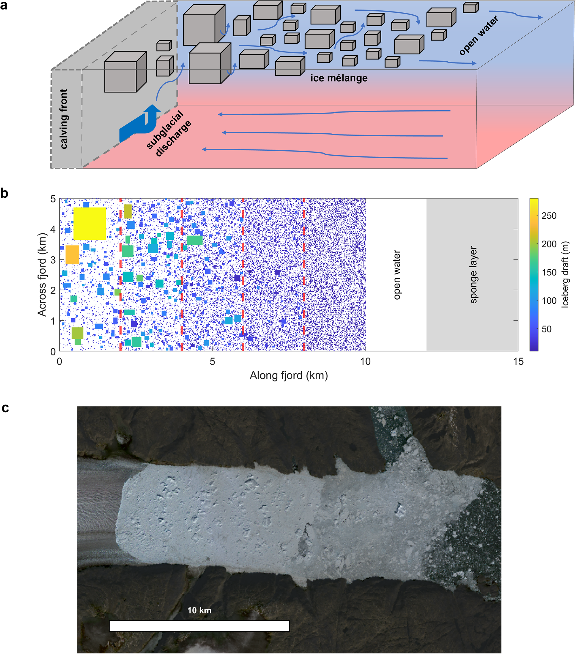
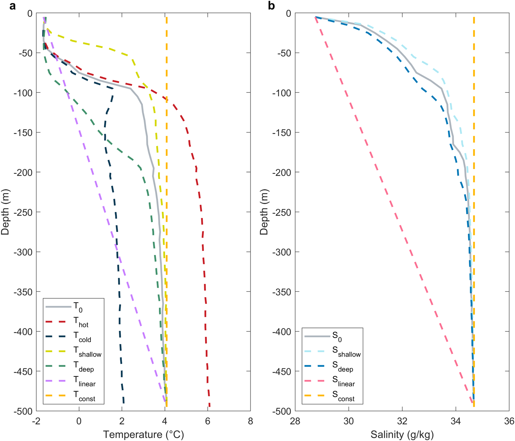


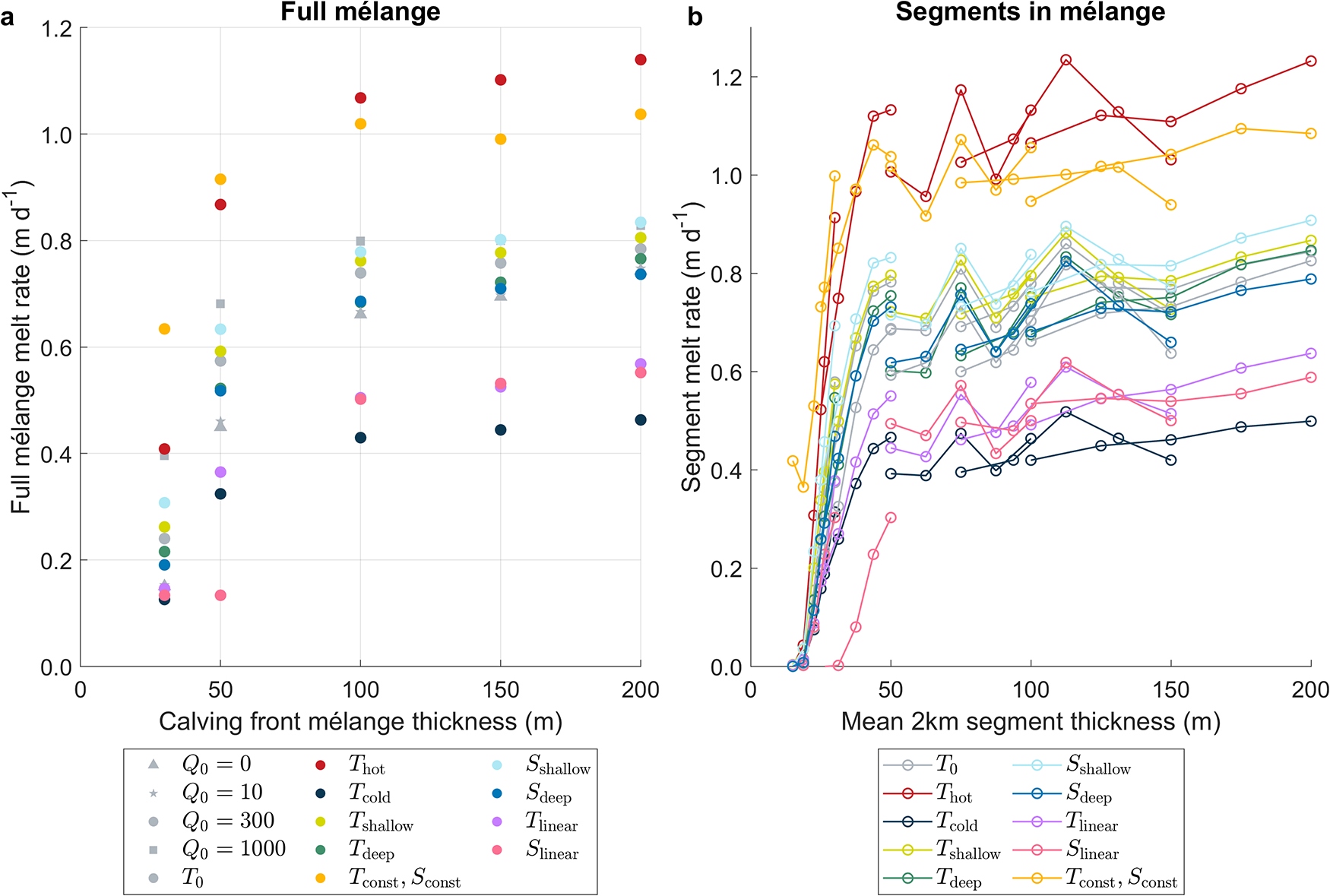


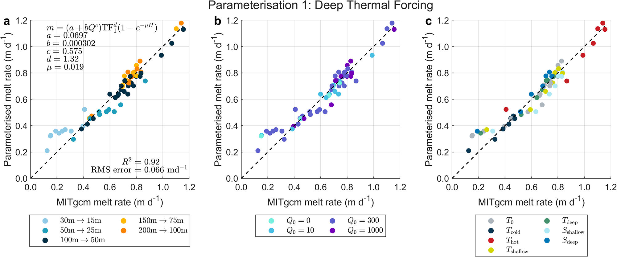

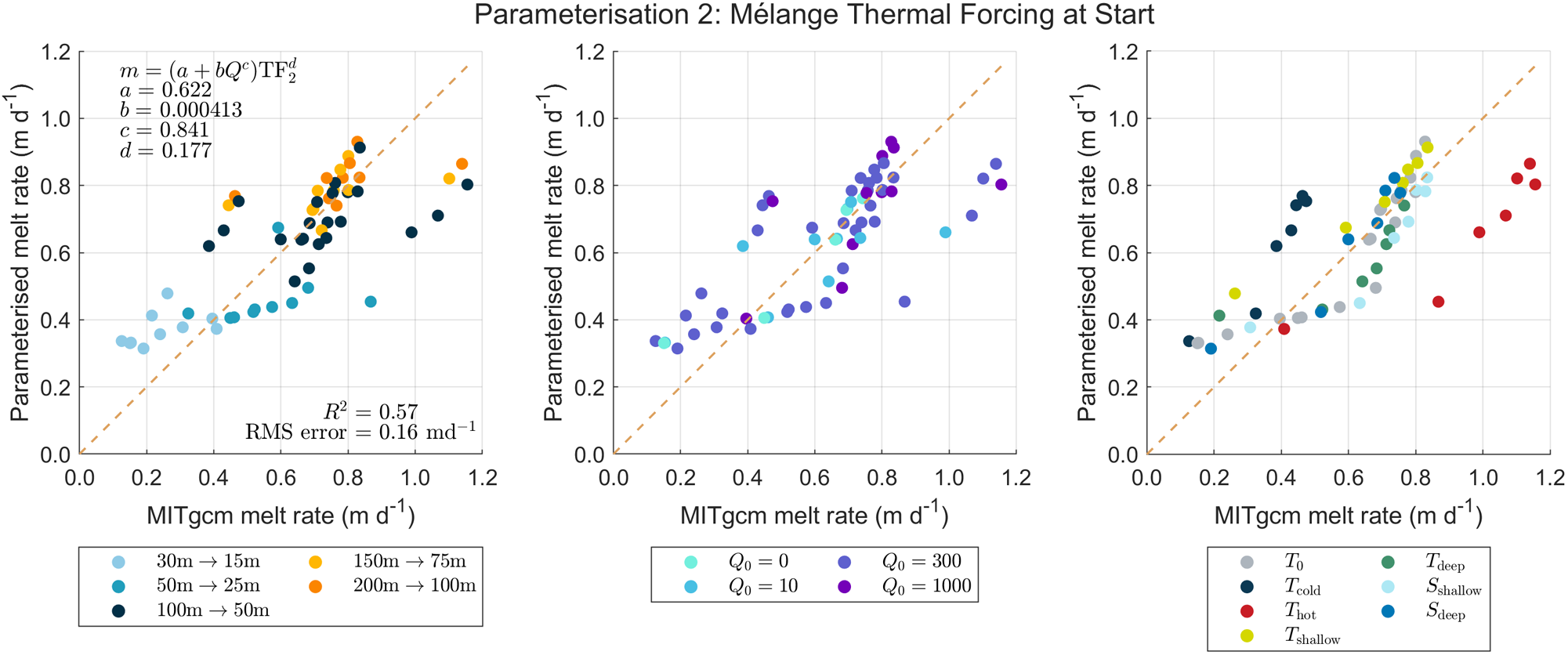

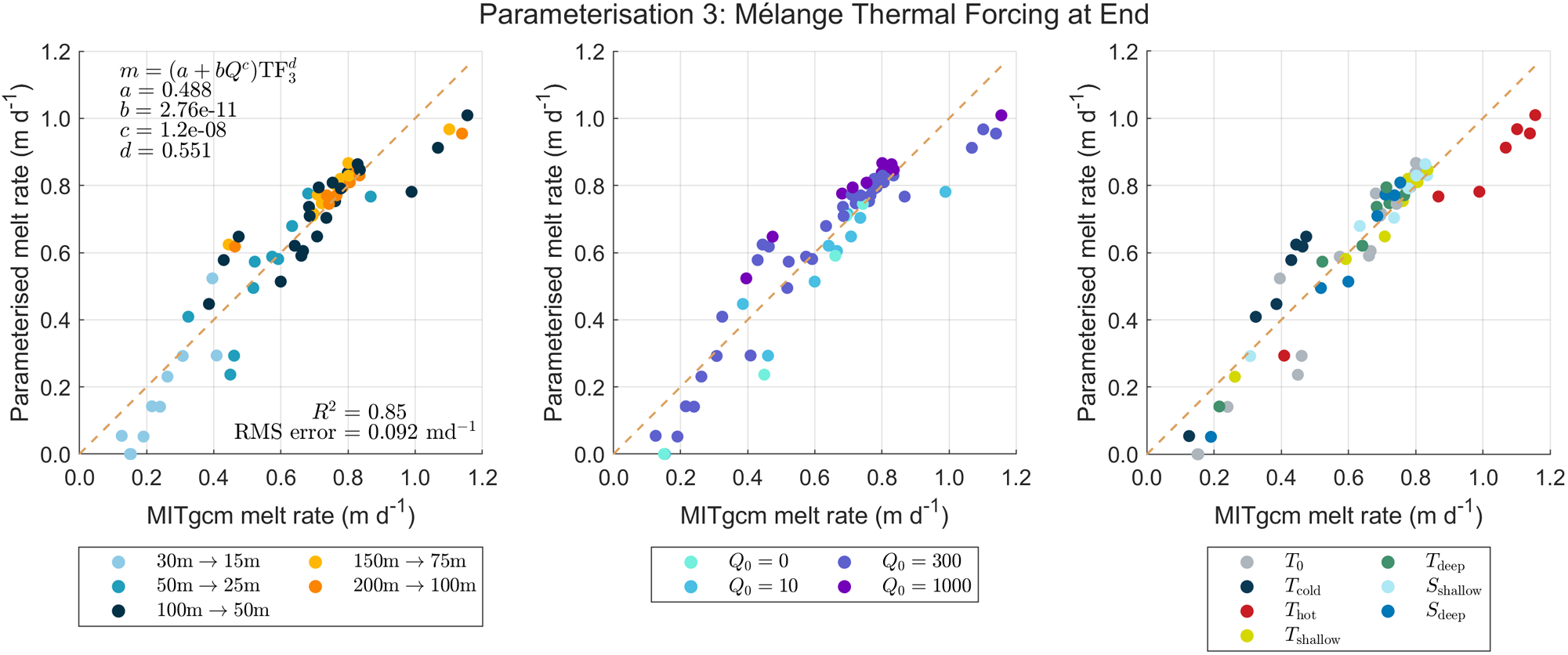

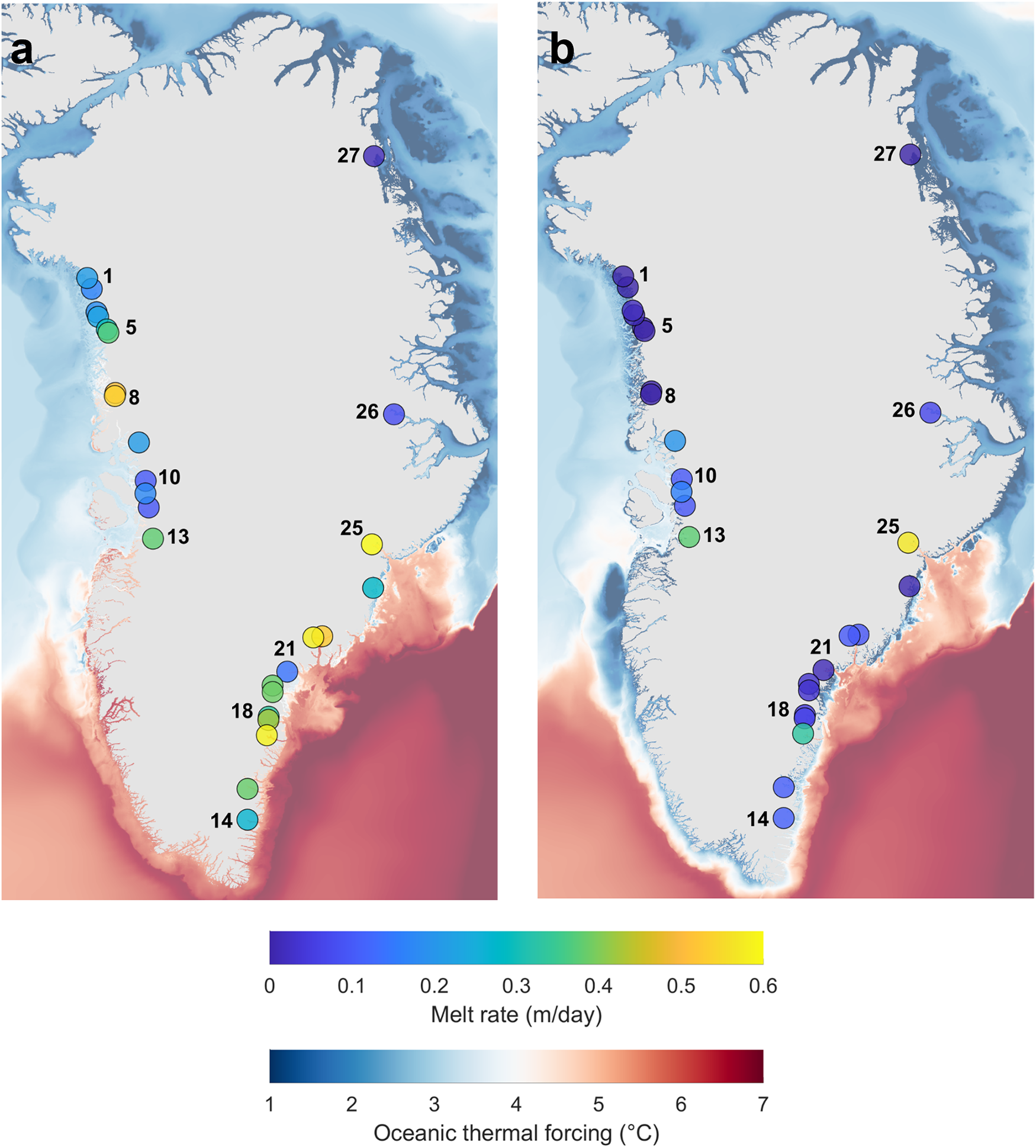

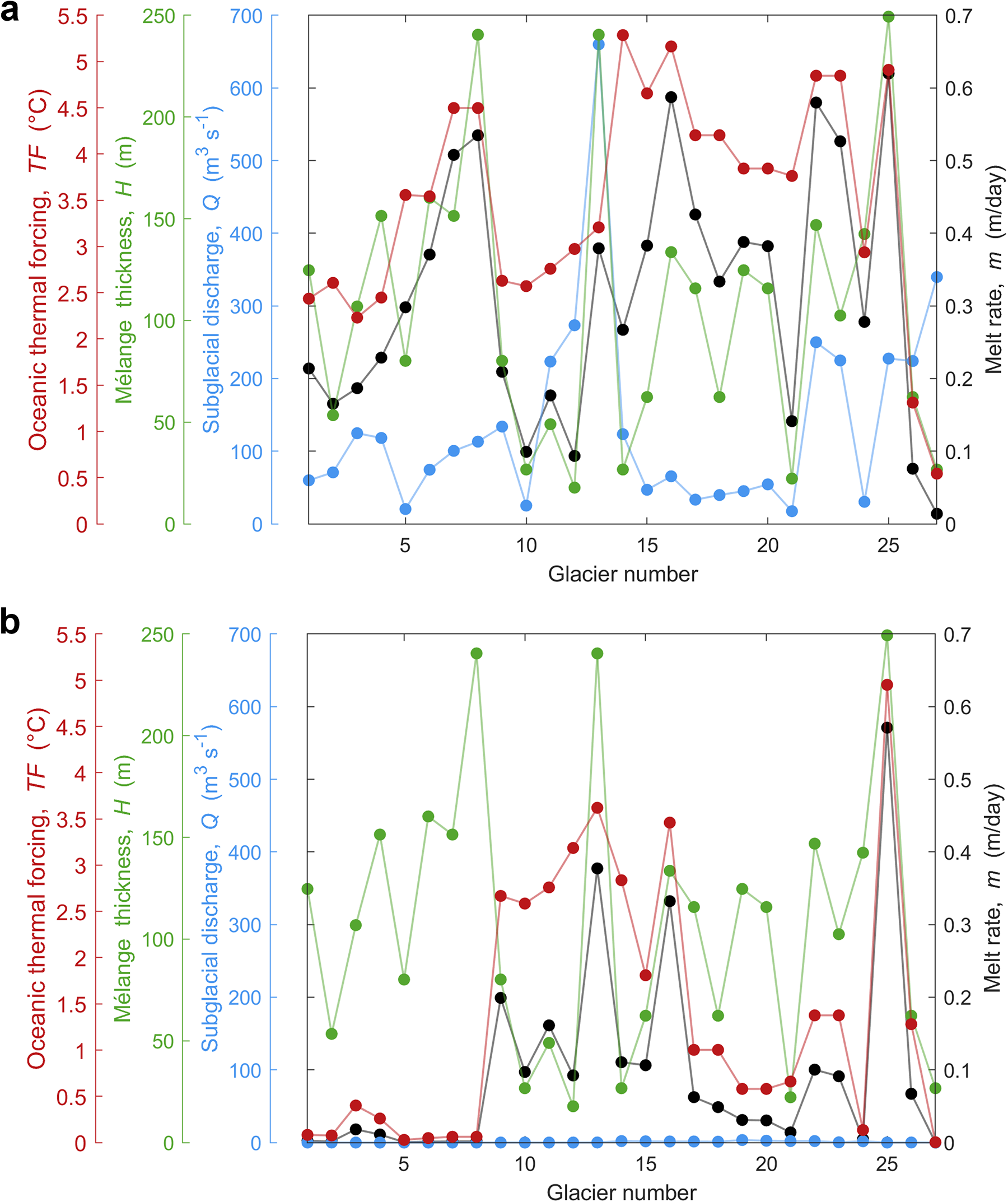

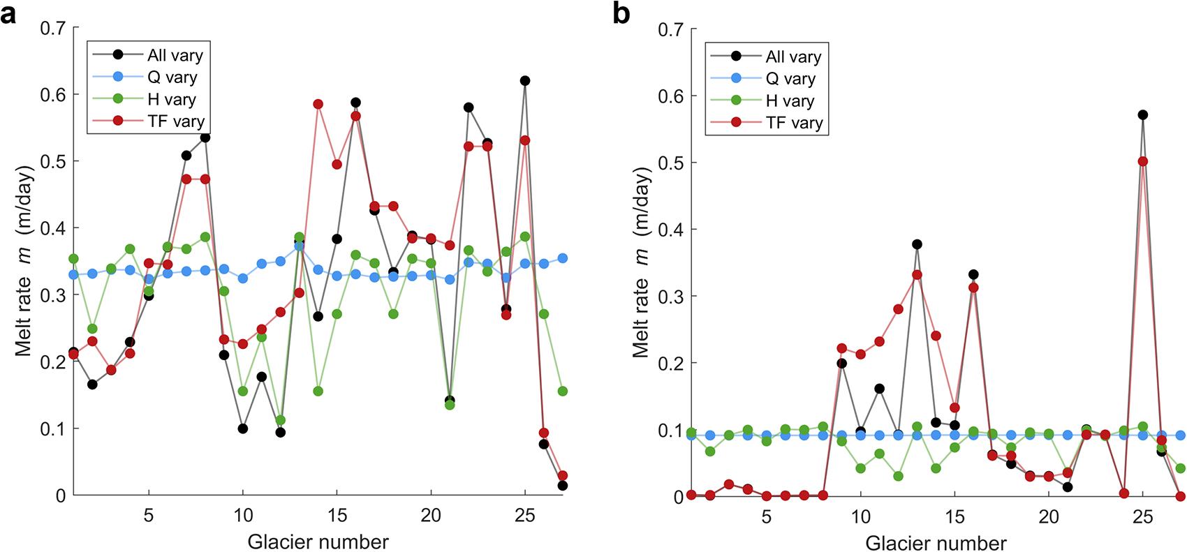
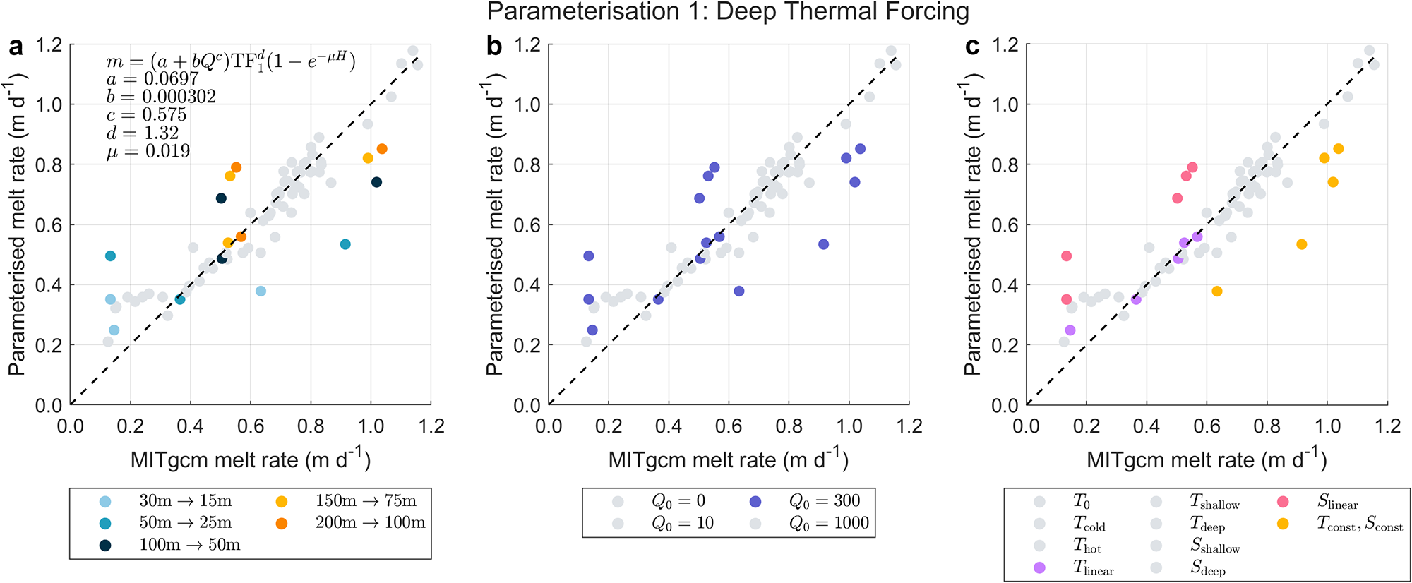


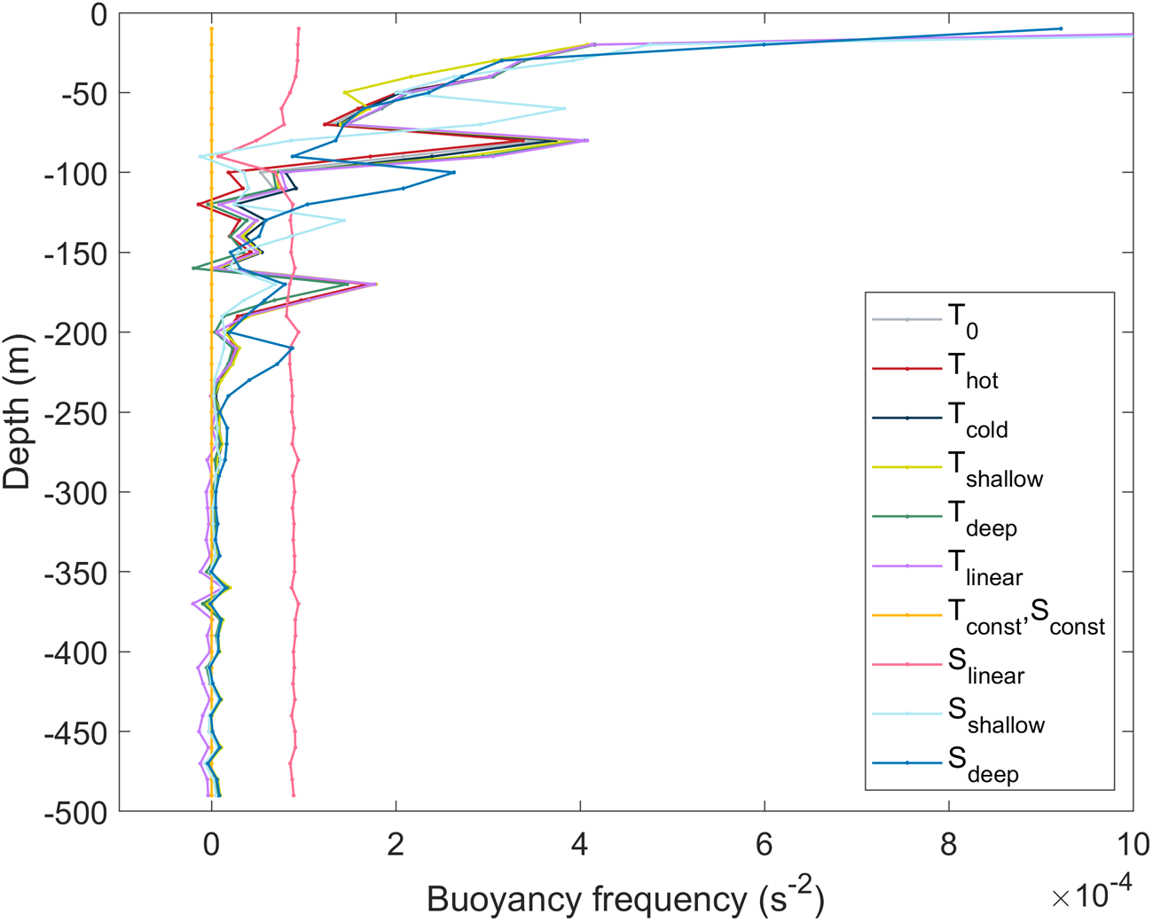

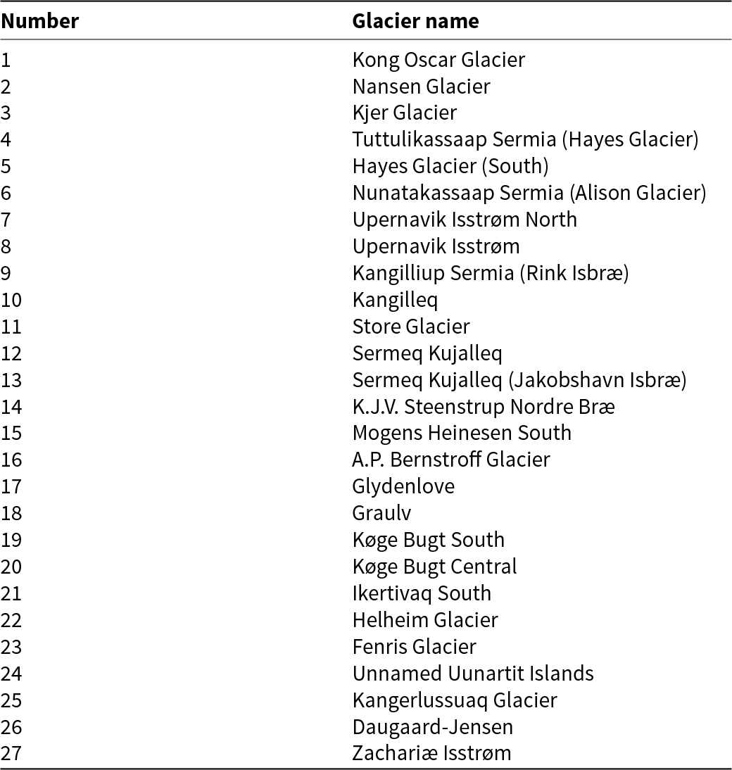




 Open access

