


1. Introduction
Venezuela offers a unique opportunity to study long-run distributional dynamics in an economy dominated by oil wealth since the 1920s. Has this abundance led to more equal income sharing among Venezuelans? Or has it instead reinforced deep-rooted historical disparities stemming from a high concentration of asset ownership? Given state ownership of subsoil resources and the central role of public oil revenues in the country’s development strategy, oil wealth was widely expected to function as a force for broadly shared prosperity and income equality. The use of “equality” in the title reflects this developmental promise. Yet a major obstacle to addressing this question is the scarcity of long-run data on inequality – particularly on capital income. Overcoming this limitation is the first task of this study; answering the pivotal question is its ultimate objective.
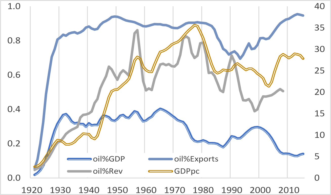
Venezuela is a textbook oil economy. Between 1920 and 2013, oil accounted on average for 80% of exports, 50% of fiscal revenues, and 30% of GDP (Figure A1). Few developing oil economies offer the possibility of analyzing income distribution over such an extended horizon. Oil wealth and oil dependence are often two sides of the same coin: while the former provides a developmental opportunity, the latter – under limited diversification – exposes the economy to severe external shocks. The trajectory of real GDP per capita reflects both realities, with a marked turning point in the late 1970s.
The analysis focuses on 1920–2013 for two reasons. First, 2013 marks the end of the first oil boom of the twenty-first century. Second, it coincides with the death of President Hugo Chávez, whose successor, Nicolás Maduro, presided over a period characterized by institutional breakdown, economic collapse, oil sanctions (from 2019), political repression, social unrest, and mass emigration. An additional consequence has been the deterioration in the production and publication of macroeconomic, labor-market, and household-survey data (Bello Rodríguez, Reference Bello Rodríguez2023), which severely constrains inequality measurement for the subsequent years using official data. Developments during 2014–2025 are nonetheless considered in the conclusions.
To overcome data constraints, I construct dynamic social tables that classify the labor force into four occupational groups defined by skill level, adapted from Astorga (Reference Astorga2024).Footnote 1 The top group (employers, managers, and professionals) concentrates capital income, whereas labor income predominates in the lower three groups (for example, clerks, masons, and laborers). This structure facilitates the identification of the income share accruing to high earners; however, it cannot meaningfully distinguish between different segments of the elite, thereby missing potential heterogeneity at the top of the distribution. Three Gini coefficients are deployed to track inequality between these groups: two pre-fiscal measures – the overall Gini (G4All), which includes all primary income sources; the labor Gini (G4Lab), based solely on labor income; and an extended, post-transfer Gini (G4Ext), which incorporates in-kind social transfers in education and health.Footnote 2 Despite the small number of groups, substantial income gaps between them – and relative homogeneity within them, except at the top – allow these measures to provide a reliable proxy for long-run inequality trajectories.
Regarding the drivers of inequality, the paper examines the role of oil rents as the main source of fiscal revenues, as well as their influence on structural transformations in the non-oil economy. It pays particular attention to the interplay between external factors linked to the international oil market and structural dynamics associated with accelerated urbanization and industrialization, rapid advances in human capital formation, and the demographic transition.
The paper examines inequality across two contrasting periods. Period 1 (1920–1973) was characterized by rapid growth driven by oil expansion, steadily rising real wages, industrialization, the consolidation of a middle class, and macroeconomic stability. Period 2 (post-1973) was marked by volatile oil rents, declining oil production, collapsing real wages after 1980, de-industrialization, middle-class erosion, and economic stagnation. The occupational Ginis reveal distinct distributional patterns across these phases, implying that conclusions about inequality dynamics are contingent both on the income measure used and the period analyzed. In Period 1, G4All narrows after the late 1950s – reflecting middle-class consolidation – while G4Lab rises due to increasing skill premiums. In Period 2, the Ginis move more closely together, except during the 1970s oil boom, which is disequalizing in G4All but equalizing in G4Lab. Crucially, while oil price shocks have distributionally asymmetric effects on overall inequality, labor inequality exhibits a sign-dependent response, narrowing during price booms but widening during slumps. Altogether, inequality proves primarily oil-driven: initially through sustained increases in production and fiscal expenditure shaping endogenous transformation, and subsequently through oil-price volatility. Although real wages grew strongly until the late 1970s, overall inequality widened during both booms and downturns, and real wages declined persistently after 1980. In-kind transfers significantly reduce the level of inequality but exert limited influence on its trajectory.
Methodologically, the paper develops a unified macro–micro framework that combines corrected national accounts, occupational dynamic social tables, and capital-income allocation to estimate long-run inequality in a resource-dependent economy. By integrating factor-income decomposition with group-level income estimation, the approach links oil-rent dynamics to occupational inequality within a consistent accounting structure. This enables construction of long-run inequality series that extend beyond conventional functional or survey-based measures, while explicitly capturing the distributive role of in-kind social transfers. To my knowledge, this is the first long-run, distributionally disaggregated inequality series for a major oil economy based on such an integrated framework.
Dominant narratives of inequality emphasize structural change in the Kuznets–Lewis tradition, globalization and trade exposure (Heckscher–Ohlin), the education–technology race (Tinbergen, Reference Tinbergen1975; Goldin and Katz, Reference Goldin and Katz2008), and institutional or political determinants of wage and wealth dispersion (Piketty, Reference Piketty2014). While these explanations identify important mechanisms, they are generally developed in contexts where market-generated income dominates, and the state plays a secondary redistributive role. In oil-dependent economies, by contrast, resource rents enter through fiscal allocation, conditioning both structural transformation and wealth accumulation – and thereby shaping how markets generate labor and capital incomes. This introduces a fundamental distributional distinction: whereas tax-financed in-kind transfers redistribute income within society, oil-financed transfers redistribute income from the rest of the world to domestic residents. The fiscal allocation of external rents therefore constitutes a central mechanism through which oil revenues shape distributional outcomes.
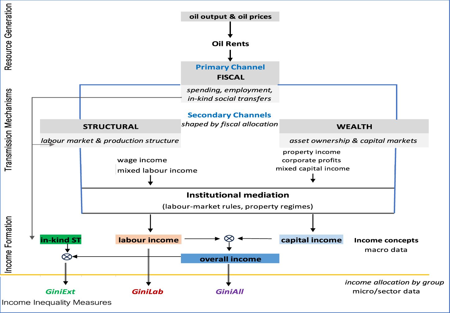
This paper proposes a layered architecture that integrates these mechanisms within a framework of fiscal primacy. Starting from the generation and allocation of Primary National Income (PNI), Figure 1 summarizes this structure by separating four analytical layers. Oil rents enter through a primary fiscal channel, which allocates resources via public expenditure, public employment, and in-kind social transfers. This allocation gives rise to two interrelated secondary channels: a structural channel, operating through labor markets, production structures, and endogenous transformations; and a wealth channel, operating through asset ownership and capital markets, where the returns generated in the production process are accumulated and distributed.Footnote 3 Institutional arrangements – including labor-market rules and property regimes – mediate how structural conditions generate labor income and how wealth generates and accumulates capital income. In-kind transfers exert both immediate distributive effects and longer-term effects by influencing human capital formation. The income flows generated through these channels constitute the components of PNI – labor and capital incomes – augmented by in-kind social transfers, which together form the basis for the labor, capital, overall, and extended income measures used to calculate the three occupational Ginis.
Fiscal primacy and the transmission channels of inequality in an oil economy.

1 Long description
The transmission channels of inequality in an oil economy. It begins with ′oil output & oil prices′ leading to ′Oil Rents′. These rents flow into the ′Primary Channel′ labeled ′FISCAL′, which includes ′spending, employment, in-kind social transfers′. From here, ′Secondary Channels′ are shaped by fiscal allocation, branching into ′STRUCTURAL′ and ′WEALTH′. ′STRUCTURAL′ involves ′labour market & production structure′, leading to ′wage income′ and ′mixed labour income′. ′WEALTH′ involves ′asset ownership & capital markets′, leading to ′property income′, ′corporate profits′ and ′mixed capital income′. Both channels are influenced by ′Institutional mediation′, which includes ′labour-market rules, property regimes′. The flow continues to ′Income Formation′, with ′in-kind ST′, ′labour income′ and ′capital income′ converging into ′overall income′. The chart concludes with ′Income Inequality Measures′ labeled ′GiniExt′, ′GiniLab′ and ′GiniAll′, representing ′income allocation by group′ and ′macro data′.
The remainder of the paper is organized as follows: Section 2 reviews the relevant literature; Section 3 introduces the oil-inequality nexus in Venezuela, summarizing developments in the oil industry and key structural transformations in the non-oil economy alongside the fiscal and structural channels; Section 4 describes the methodology applied to measure income inequality using PNI and the derivation of extended income; Section 5 presents and discusses the inequality evidence together with comparisons with alternative estimates, and incorporates the distributional impact of in-kind social transfers in Period 2; Section 6 gathers the conclusions. An Appendix includes complementary figures and tables, whereas an Online Appendix (OA) offers methodological and estimation details, and shows the results of robustness’ checks on changes in key assumptions.
2. Literature review
When studying inequality in commodity-dependent economies, it is necessary to distinguish between oil and minerals – non-renewable resources characterized, in most cases, by capital-intensive production – and agricultural commodities, which are renewable resources dominated by labor-intensive production. There are two main reasons for this. The first relates to the ownership of the resource. A large share of the output value of oil and minerals represents an economic rent – that is, the surplus accruing in excess of payments to labor and a normal return to capital. In countries where the state owns subsoil resources, a substantial proportion of this rent can be readily captured to boost public revenues, whereas in the case of agricultural commodities, any rent accrues primarily to private landowners. The second reason is that non-renewable resources, and oil in particular, have experienced a much higher price volatility compared to other commodities.Footnote 4
Of particular interest is the inequality impact of oil shocks. Theoretically, the direction of this relationship is ambiguous. A sustained rise in oil prices primarily benefits oil multinationals and/or the state as resource owner. Domestic spending of oil windfalls tends to shift relative prices in favor of non-tradable over tradable goods and their respective factors of production. Profits often rise during public infrastructure booms and in protected manufacturing firms, disproportionately benefiting capital income. The effect on labor income depends on the skill intensity of production: if non-tradables are relatively low-skill (e.g., day laborers), the skill premium may fall following a positive price shock, producing an equalizing effect (Galiani et al., Reference Galiani, Heymann and Magud2010). Because these effects can act on inequality differently, the net impact must be determined empirically.
I summarize two representative multi-country econometric studies. Mohtadi and Castells-Quintana (Reference Mohtadi and Castells-Quintana2021) analyzed a panel of 80 countries from 1990 to 2016 and found that positive price shocks in capital-intensive commodities increase inequality, as measured by household budget surveys (HBSs), with oil and mineral price hikes benefiting capital income over wages. Goderis and Malone (Reference Goderis and Malone2011) examined inequality following commodity booms, predicting a short-term decline in inequality after a price increase, followed by a gradual rise, and the reverse after a slump. Testing this with panel data from 90 mostly commodity-exporting countries (1965–1999) also using HBS, they confirmed the pattern for oil and mineral booms but found negative shocks statistically insignificant, suggesting an asymmetric distributional effect.
Some reasons behind the apparent contradiction in the findings are differences in methodology, country sample, and time coverage. But, leaving that aside, notice that, because of the gross underestimation of capital income in HBS, the results of these studies largely inform us about labor income inequality and may not accurately capture overall income inequality.Footnote 5 A more serious limitation of panel data studies is scarcity of survey or tax data informing on income inequality in the majority of oil countries in the Middle East – except Iran – since 1980 or earlier (Adams and Page, Reference Adams and Page2003). This is compounded by the fact that when household surveys are available in oil producers in sub-Saharan Africa, they tend to measure consumption (Gasparini and Tornarolli, Reference Gasparini and Tornarolli2009).
The ambiguity of the results in panel-data studies and their data limitations call for focusing on country experiences in oil and mining economies. One salient example is Bhattacharyya and Williamson (Reference Bhattacharyya and Williamson2016), who looked at the inequality outcome of commodity price shocks in Australia between 1921 and 2008 using tax data to capture capital income. They found that the very top end of the income distribution benefited disproportionately during non-renewable booms. Farzanegan and Krieger (Reference Farzanegan and Krieger2019) examine the inequality response to positive oil and gas revenue shocks in Iran (1973–2016) using HBS. They find that income inequality widens in the short run, driven by private-sector credit expansion and construction booms. However, the study remains silent on inequality dynamics during revenue slumps.
In Venezuela, the oil–inequality nexus has been extensively examined (Urdaneta, Reference Urdaneta de Ferrán1977; Bourguignon, Reference Bourguignon, De Bandt, Mándi and Seers1980; Musgrove, Reference Musgrove1981; Valecillos, Reference Valecillos1989; Maza Zavala, Reference Maza Zavala1991; Freije, Reference Freije, Hausmann and Rodríguez2014), primarily using consistently defined household surveys available since 1974. Because these surveys routinely only included labor income, they grossly underestimate top incomes. Gini coefficients based on this evidence show a sharp decline in inequality during the oil boom of the 1970s and early 1980s, pronounced volatility in the late 1980s, rising inequality in the 1990s, and a renewed narrowing during the 2000s boom (Figure 4). To address the omission of capital income, several studies focus on functional inequality. A seminal contribution is Baptista (Reference Baptista1980, Reference Baptista1985), who develops a framework for analyzing oil-rent distribution and argues that oil booms raise returns to capital in the non-oil economy – particularly manufacturing under import substitution from 1953 to 1978. He finds that a substantial share of oil rents accrued as abnormal profits, suggesting a disequalizing effect of the 1970s boom. Rodríguez (Reference Rodríguez and Cornia2004) reports a stable functional inequality between 1971 and 1982, followed by a rise up to 1997. The most comprehensive analysis in terms of period (1975–2004) and income coverage is Baptista (Reference Baptista and Giordani2006b), who estimates capital income using national disposable income and total remunerations; this work is examined further in Section 5 and the OA.
3. The oil-inequality nexus in Venezuela
During the period under analysis, developments in the oil industry and income distribution were closely intertwined. In the early decades, the impact was direct, operating through investment and labor demand, particularly for largely unskilled workers required to develop oil fields. This effect was especially significant during the initial phase of Period 1, when extensive transport and communications infrastructure had to be built (McBeth, Reference McBeth1983). Moreover, following the establishment of the first trade union in 1936 (Salazar Zaíd, Reference Salazar Zaíd2021), oil workers secured substantial improvements in wages, working conditions, and social protection. These advances subsequently served as a model for labor organization and the extension of rights – most notably social security – to non-oil formal sectors during the 1950s and 1960s. Oil-sector wages were also significantly higher than those elsewhere, with managers and professionals typically located in the top decile of the income distribution (Harris, Reference Harris and Mikesell1971).
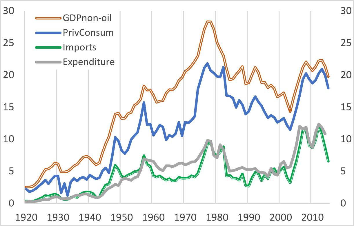
From the 1950s onward, however, the oil sector increasingly functioned as a capital-intensive enclave with limited labor demand and weak direct linkages to the non-oil economy. Its main distributional impact therefore operated through the fiscal channel, as oil rents expanded government revenues and expenditure, particularly on public services and infrastructure, while the structural channel worked mainly through the creation of jobs and economic diversification. At the same time, oil rents generated the foreign exchange required to finance imports and sustain domestic consumption (Figure A2), rendering non-oil activity highly dependent on – and vulnerable to – oil shocks. Given the high import content of production, the non-oil tradable sector was unable to generate sufficient foreign exchange and instead relied on oil revenues. Government spending completed the cycle by stimulating domestic demand and supporting firm profitability.
Consequently, Venezuela represents an extreme case of oil-rent-driven macroeconomic and fiscal pro-cyclicality. Given the central role of the fiscal channel and the absence of effective and lasting stabilization instruments,Footnote 6 oil price volatility – especially after 1973 – was transmitted into domestic economic activity in general, and into employment and remuneration in particular. This limited the government’s capacity to use fiscal and social policies to dampen the inequality effects of oil shocks, which therefore had pronounced distributional consequences, as discussed in Section 5, consistent with evidence of strongly procyclical fiscal dynamics in Venezuela.
Beyond contemporaneous macroeconomic dynamics, oil-driven expenditure also shaped long-term structural transformations, including the demographic transition, human capital formation, internal migration and urbanization, (de)industrialization, and institution-building. In particular, public spending on sanitation, health, and education was central to the first two processes. These transformations were gradual and path-dependent, with significant distributional effects operating primarily through the structural channel. Although similar changes occurred across Latin America in the late twentieth century (Astorga et al., Reference Astorga, Bérges and FitzGerald2005), in Venezuela their timing, pace, and form were decisively shaped by the country’s distinctive oil wealth. Moreover, the inequality effects associated with oil dependence were mediated by fluctuations in international oil markets, which could abruptly alter prices and production.
Understanding Venezuela’s inequality dynamics therefore requires analyzing the interaction between endogenous structural transformations and external oil shocks. The following section documents developments in the oil sector alongside changes in the non-oil economy, highlighting the central role of the fiscal and structural channels. The wealth channel is examined in greater detail in Sections 4 and 5.
3.1. The oil sector and the fiscal channel
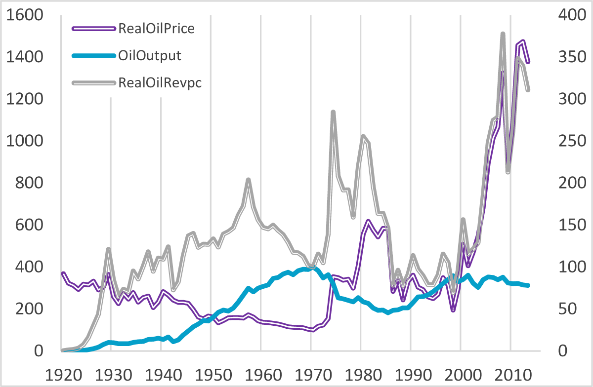
The evolution of Venezuela’s oil sector can also be divided into two broad periods, with 1973 as the watershed. This break reflects the geopolitical shock of the Yom Kippur War, which fundamentally reshaped the international oil market. As shown in Figure 2, Period 1 is characterized by a steady increase in oil production – particularly since the early 1940s – largely at the hands of oil multinationals, relatively stable oil prices under their control, and a gradual rise in the state’s claim on oil profits (Baptista and Mommer, Reference Baptista and Mommer1987; Manzano, Reference Manzano, Hausmann and Rodríguez2014). Real oil fiscal revenues per capita rose 2.2 times between the early 1930s and c.1960.Footnote 7 But the 1960s saw a 30% decline in real revenues per capita, reflecting falling real oil prices and rapid population growth.
Real oil price, oil production, and real oil revenues per capita.

In October 1973, the Arab countries of the Organization of the Petroleum Exporting Countries (OPEC) – of which Venezuela was a founding member in 1960 – implemented an oil embargo that triggered a fourfold hike in international oil prices. This event marks the start of Period 2. The surge in oil rents boosted domestic income and, in turn, consumption and imports (Figure A2). It also financed the nationalization of the oil industry in January 1976. Control was transferred to the newly created state-owned company Petróleos de Venezuela Sociedad Anónima (PDVSA), making the state the direct recipient of oil revenues and significantly enhancing its influence over income distribution.
The second period is marked by medium-term fluctuations in oil production and highly volatile prices. In March 1983, OPEC adopted production quotas to support prices, prioritizing rent maximization over output expansion. In Venezuela, this led to a decade of stagnating or declining production, reaching a historical low between 1986 and 1989, and contributing to weaker economic growth given the sector’s large share in GDP (Figure A1).
Production recovered in 1992, when Carlos Andrés Pérez’s government reopened the sector to foreign firms through joint ventures and service contracts under the Apertura Petrolera. This reform boosted production capacity, offsetting declines in PDVSA output and sustaining higher output levels throughout the 1990s. However, low oil prices and rapid population growth prevented this expansion from translating into higher per capita revenues. In 2001, Hugo Chávez’s government enacted a new Hydrocarbons Law that strengthened state control by requiring PDVSA to hold a minimum 51% stake in all exploration and production projects. Although output remained broadly stable during the 2000s and declined sharply in the 2010s, rising oil prices substantially increased fiscal revenues.
While longer-term movements in production shaped the baseline for revenues and economic activity, oil-price volatility dominated Period 2. This included the boom of the 1970s, a further windfall in 1980–1981 triggered by the Iran–Iraq War, and the 2003–2013 upswing driven by rising demand from China. Conversely, major price collapses occurred in 1986–1989 owing to global oversupply, in 1998, and during the Global Financial Crisis of 2009. As Figure 2 shows, this volatility translated into sharp swings in fiscal revenues. Moreover, heavy external borrowing during the boom meant that, following the 1982 debt crisis, a substantial share of public income was absorbed by external debt servicing.Footnote 8 The resulting contraction in expenditure weakened the distributive capacity of the fiscal channel and had an immediate negative impact on non-oil activity and labor-market conditions, generating job losses and falling real wages.
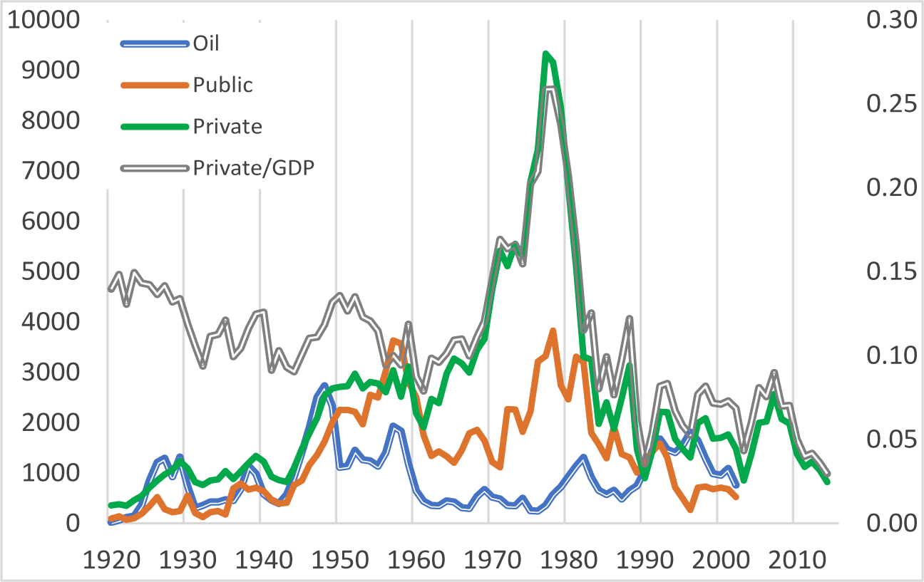
Although the oil boom of the 2010s supported a recovery in economic growth and a moderate rise in real wages, private physical investment remained subdued (Figure A3), reflecting heightened legal uncertainty. As a result, the boom failed to resolve the labor market’s structural weaknesses. A key difference between the windfalls of the 1970s and 2000s lies in their composition: while the former was largely invested in human and physical capital, supporting labor absorption, the latter primarily financed consumption (Figures A.2 and A.3). Consequently, the earlier boom generated stronger employment and wage-equalizing effects, whereas the later episode produced a more limited and fragile reduction in labor inequality, with a more prominent role for social transfers.
3.2. Structural transformations and the structural channel
Around 1920, Venezuela was predominantly rural, poorly educated, and at an early stage of the demographic transition. Economic activity was weakly diversified, with an incipient manufacturing base and an export structure concentrated in a narrow range of agricultural commodities – chiefly coffee and cocoa – which dominated export revenues prior to the rise of oil. Over subsequent decades, profound structural transformations reshaped the economy with far-reaching distributional consequences (Astorga, Reference Astorga, Cárdenas, Ocampo and Thorp2000).
The country underwent a classic demographic transition, as improvements in sanitation and public health reduced mortality and supported rapid population growth in the middle decades of the twentieth century. Labor‑force participation expanded from about 44% in 1970 to 56% in 1980, reaching over 61% by 2000 (PREALC 1982; ECLAC 2025), as larger cohorts entered the labor market. This created the conditions for a rise in labor informality – increasingly important after the mid-1980s – undermining real wages, particularly for unskilled workers.
Education attainment rose in parallel. After the restoration of democracy in 1958, primary school enrolment expanded rapidly and stabilized by the late 1960s. Thereafter, tertiary education grew exponentially. By the mid-1970s, this growth – supported by rising public spending and a marked shift towards higher education (Kornblith and Maingón, Reference Kornblith and Maingón1985) – reinforced a bias toward university studies and boosted the supply of highly skilled workers. Average years of schooling in the labor force rose from 2.9 in 1960 to 6.6 by the 1990s. However, improvements in educational quality lagged behind quantitative expansion, particularly after the 1980s, when declining funding and institutional capacity reduced the skill content of each additional year of schooling (Ortega and Pritchett, Reference Ortega, Pritchett, Ricardo Hausmann and Rodríguez2014; ECLAC 2025).
Structural change accelerated internal migration and urbanization, raising the urban population from around 16% in 1920 to over 70% by 1980 (Baptista, Reference Baptista2006a). Workers moved into construction, services, and manufacturing, while the rural share of the economically active population (EAP) fell from 46% in 1950 to 19.5% by 1980 (PREALC 1982). The urban–rural literacy gap narrowed sharply, with the ratio declining from 2.52 in the 1940s to 1.42 in the 1980s (Astorga, Bergés, & FitzGerald Reference Astorga, Bérges and FitzGerald2005). Incomes in urban services and manufacturing relative to agriculture rose between 1936 and 1959 but fell in the closing decades of the century (Valecillos, Reference Valecillos2007). Consistent with the Kuznets–Lewis framework, these trends suggest that surplus labor was initially absorbed into higher-productivity activities, narrowing sectoral wage gaps.
State-led import-substitution industrialization, initiated in the 1950s and expanded during the 1960s, promoted manufacturing diversification but sustained a largely oligopolistic structure with concentrated profits in a small domestic market with limited foreign competition, reinforcing inequality through the wealth channel. In the 1970s, policy shifted toward resource-based industrialization, particularly in export-oriented basic metals. From the late 1970s onward, declining investment, weakening competitiveness, and adverse external shocks triggered industrial contraction (Bourguignon, Reference Bourguignon and Gelb1988; Vera, Reference Vera2009), displacing labor into low-productivity informal services and amplifying inequality via the structural channel. Under advanced urbanization, labor-market segmentation increasingly reflected the formal–informal divide rather than the earlier rural–urban cleavage, linking sectoral dynamics directly to inequality patterns discussed in Section 5.
Labor‑market institutions evolved alongside these structural shifts. Organized labor emerged early, with the establishment of the first trade union in the oil sector in 1936. Union density and collective bargaining power strengthened steadily, peaking at around 45% in the late 1970s, before declining sharply to below 15% by the early 2000s (Valecillos, Reference Valecillos1986; Lucena, Reference Lucena and de la Garza Toledo2005). Minimum wages, introduced in 1974, rose moderately until the mid-1980s but subsequently eroded in real terms; by the late 2000s, the minimum wage stood at only about 70% of its 1974 level (Riutort and Balza, Reference Riutort and Balza2001).
The distributional effects of these long-run transformations primarily operate through the structural channel. Demographic change and educational expansion shape skill supply, which, together with labor demand and technological change, determines wage premiums. Structural transformation influences the level and sectoral composition of labor demand, while labor-market institutions mediate wage-setting and the division between profits and wages. These mechanisms, together with the contemporaneous effects operating through the fiscal channel, jointly govern employment patterns – particularly informality, wage dispersion, and the labor share – thereby shaping labor and overall income inequality. The next section develops the methodology used to examine these effects empirically.
4. Measuring income inequality
To analyze how oil rents affected income distribution, I construct overall, labor, and extended Gini coefficients starting from the standard National Accounts decomposition of national income at factor cost (primary income)Footnote 9:
 \begin{equation}\text{Yfc = W + GOS + MI}\end{equation}
where Yfc denotes national income at factor cost, W is compensation of employees (i.e., labor income of salaried workers), GOS is gross operating surplus, and MI is mixed income from self-employment and unincorporated enterprises. A well-known limitation of this decomposition is that mixed income combines both labor and capital returns. Assigning all of MI to capital therefore biases factor shares by overstating capital income and understating labor income. Following the standard correction in the literature (Gollin, Reference Gollin2002), mixed income is split into a labor component (MIL) and a residual capital component (MIK),Footnote 10 yielding:
 \begin{equation}\text{Yfc = W + MIL +}\left[ \text{GOS + MIK} \right],\end{equation}
where  ${\text{MIL =} \alpha\text{MI; MIK = }}\left( {{\text{1 -}\alpha}} \right){\text{MI; }}\alpha \in \left[ {{\text{0,1}}} \right]$.
4.1. Oil rents and factor incomes
In oil economies, resource rents are recorded partly as explicit royalties and partly as operating surplus in the oil sector. Since separating normal returns to capital from pure rents is empirically infeasible over long historical periods, I follow standard practice and treat the entire operating surplus of the oil sector, together with royalties, as oil rents (Roil). Accordingly,  ${\text{GOS = GOSnoil + Roil}}$ so that:
 \begin{equation}\text{Yfc = W + MIL +}\left[ \text{GOSnoil + Roil + MIK} \right]\end{equation}
In Venezuela, where the oil sector has been dominated by the state-owned company PDVSA since nationalization in 1976, a substantial share of oil rents accrues directly to the government through profits, royalties, and fiscal transfers. I therefore decompose oil rents into government and private components:
 \begin{equation}\text{Roil = Rg + Rp,}\end{equation}
where Rg represents government rents (via PDVSA and taxation), and Rp represents any residual accruing to private actors (oil multinationals pre-nationalization and after the Apertura Petrolera of 1993). Substituting equation (4) into equation (3) yields:
 \begin{equation}\text{Yfc = W + MIL +}\left[ \text{GOSnoil + Rg + Rp + MIK} \right]\end{equation}
4.2. Extended income and social transfers in kind
In rentier economies, a large share of public expenditure, particularly in-kind social transfers such as public healthcare and education (STiK),Footnote 11 is financed out of government oil rents. Beyond their long-run effects on human capital, these transfers have immediate and contemporaneous distributional consequences. To capture these effects, I explicitly incorporate in-kind social transfers into the income concept used to measure occupational inequality (Atkinson, Reference Atkinson2015).
Specifically, I define extended national income at factor cost as:
 \begin{equation}\text{Yfc = W + MIL + STiK +}\left[ \text{GOSnoil + Rg + Rp + MIK - STiK} \right]\end{equation}
This expression leaves total income unchanged, but reallocates in-kind social transfers from capital income – where they originate, via government oil rents – to labor income, where they are ultimately received by households. Equation (6) thus provides the accounting basis for distinguishing between primary (pre-transfer) income and extended primary income, explicitly capturing the distributive role of public service provision. Without this adjustment, these transfers would remain hidden within the capital share and, worse, would be allocated in line with private capital income, introducing a substantial inequality bias.
4.3. Functional income shares
Two important measures that can be derived from equation (6) are the capital and labor shares of income, which measure functional inequality. The capital share is defined as:
 \begin{equation}\text{CI}\%\text{ =}\left[ \text{GOSnoil + Rg + Rp + MIK - STiK} \right]\text{/ Yfc \times100,}\end{equation}
and the labor share as:
 \begin{equation}\text{LI}\%\text{ =}\left[ \text{W + MIL} \right]\text{/Yfc \times100}\end{equation}
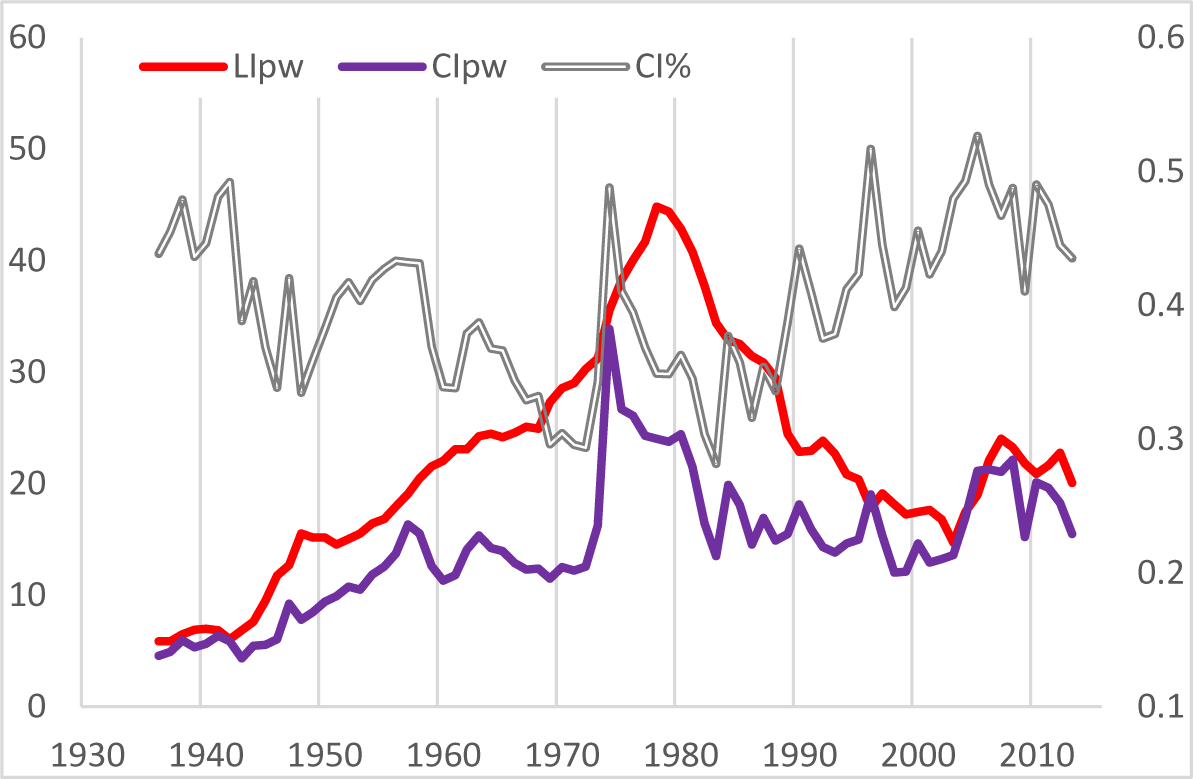
By excluding in-kind social transfers from both numerators, these shares are calculated on the basis of primary income, consistent with standard national-accounts practice. Figure 3 plots the capital share alongside real labor and capital income per worker.
Total labor income and capital income per worker.

Figure 3 Long description
Three lines representing real labour income (LIpw), real capital income (CIpw) and capital share (CI percent) over time from 1930 to 2010. The horizontal axis is labeled with years ranging from 1930 to 2010. The left vertical axis represents income values from 0 to 60, while the right vertical axis represents capital share values from 0.1 to 0.6. The red line indicates LIpw, showing an increase from 1930, peaking around 1980 and then declining. The purple line represents CIpw, which rises steadily until around 1980, then fluctuates. The grey line shows CI percent, which fluctuates throughout the period. Key data points include: LIpw peaks around 1980, CIpw rises steadily until 1980 and CI percent fluctuates throughout. The legend identifies each line with its corresponding metric.
Although functional income shares are widely used in the literature, they have two main limitations for analyzing interpersonal inequality. First, they implicitly assume that individuals derive income from a single source. Second, they abstract from inequality within both labor and capital components. In this study, functional inequality therefore serves primarily as a complementary indicator, helping to contextualize the trajectories of overall and labor inequality, which form the core focus of the analysis in Section 5. The distributional effects of in-kind social transfers are examined explicitly in Section 5.2.
4.4. Occupational Ginis
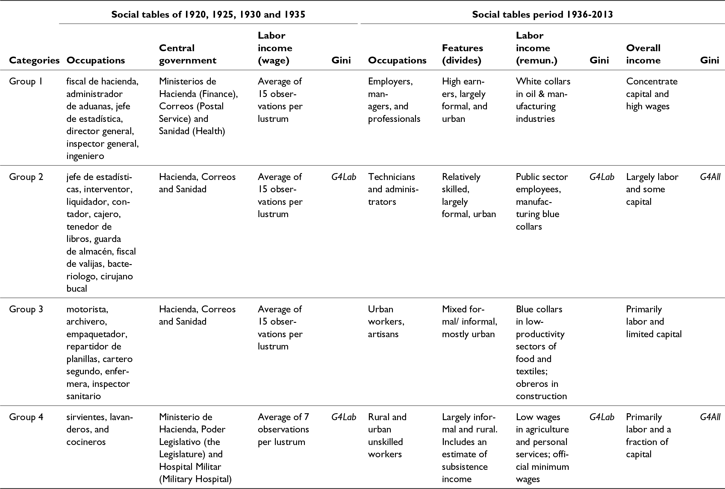
To measure income inequality, I construct dynamic social tables based on four occupational groups. The EAP is divided into:
• Group 1: Employers, managers, and professionals.
• Group 2: Technicians and administrators.
• Group 3: Semi-skilled workers and other urban workers in low-productivity sectors (e.g., retail and transport).
• Group 4: Urban and rural unskilled workers, including domestic servants.
These groups are based on the categories used in ECLAC’s Social Panorama (2000) and correspond closely to standard International Labor Organization classifications (Table A1). To ensure consistency with the aggregate EAP series, the labor force in Group 3 is calculated as a residual.Footnote 12
To calculate average labor income per group, I rely on representative series of remunerations per worker designed to capture differences in skill intensity.
Group 1 combines white-collar remunerations in the oil and manufacturing sectors, excluding the low-productivity activities of food, textiles, and footwear. This average proxies the remunerations of managers, professionals, and the mixed income of self-employed professionals in the wider economy. Earnings of employers are treated entirely as capital income.
Group 2 uses a weighted average of mean remuneration in the public sector and in manufacturing (excluding low-productivity activities). This group consists mainly of formal workers, with a small number of self-employed professionals whose mixed income is proxied by the group average.
Group 3 combines average remunerations in construction with those in food, textiles, and footwear.
Group 4 draws on unskilled wage series, distinguishing between urban and rural areas where possible. The mixed income of unskilled self-employed workers in Groups 3 and 4 is proxied by the respective group averages (Online Appendix 2).
To estimate mean capital income by group, I begin with aggregate non-oil capital income derived from equation (6), which adjusts for mixed income and excludes in-kind social transfers. This total is allocated across the four groups using detailed data on property income around 1960, disaggregated by income brackets, from Urdaneta (1977), under the assumption of a stable relative distribution over time (OA.1). Undistributed profits before corporate taxes are allocated in proportion to property income. This allocation underpins the wealth channel.
Based on this occupational structure of the labor force, and the labor and capital income per group, I compute three Gini coefficients to measure income inequality between the four groups.Footnote 13
Labor Gini (G4Lab): Captures inequality in labor income under the assumption that all individuals within each group receive the group means. For a given year t, it is defined as:
 \begin{equation*}G4Lab = \sum \limits_{i = 2}^{4}\sum \limits_{j = 1}^{i-1}e{'_j}e{'_i}\left| r{'_j}-r{'_i} \right|,\end{equation*}
where e′i denotes the EAP share of group i, and r′i is the ratio of the mean labor income of group i to the mean labor income across all four groups, and e′ir′i equals the labor-income share of group i (s′i).
Overall Gini (G4All): Measures total income inequality assuming that all individuals within each group receive the group mean total income. For a given year t, it is computed as:
 \begin{equation*}G4All = \sum \limits_{i = 2}^{4}\sum \limits_{j = 1}^{i-1}{e_j}{e_i}\left| {r_j}-{r_i} \right|,\end{equation*}
where ei is the EAP share of group i; ri is the ratio of the mean total income of group i to the mean total income across the entire EAP (income per person engaged), and eiri equals the total income share of group i (si) (OA.4).
To obtain group mean total income for the overall Gini, I reconcile group-level wage series with aggregate labor income from the national accounts (equation (2)). Specifically, average real labor income per group is recalculated by applying the group’s labor-income share (s′i), derived from the remuneration series, to aggregate labor income (Appendix 1.2). This adjustment reduces group-level averages relative to raw wage data but preserves labor-income inequality and ensures full consistency with macro aggregates.
Extended Gini (G4Ext): Incorporates in-kind social transfers to capture the broader economic claim of occupational groups on national income. For a given year t, it is computed analogously to G4All, using the mean extended income of each group (labor + capital + in-kind social transfers):
 \begin{equation*}\sum \limits_{i = 2}^{4}\sum \limits_{j = 1}^{i-1}{e_j}{e_i}\left| r'{'_j}-r'{'_i} \right|,\end{equation*}
where ei is the EAP share of group i; and r″i denotes the ratio of mean extended income of group i to mean extended income across the entire EAP.
This formulation allows G4Ext to reflect the contemporaneous inequality-reducing effects of in-kind social transfers while maintaining the same four-group occupational structure.
4.5. Key estimation issues
Before presenting the evidence, some clarifications are in order.
First, I use the concept of well‑apportioned groups to assess whether the four occupational categories provide an appropriate breakdown of the EAP that minimizes potential income overlap. For a group to have a distinct identity, differences in incomes within the group should be smaller than those across groups, and the weighted sum of within‑group Ginis should not exceed the between‑group Gini (Milanovic et al., Reference Milanovic, Lindert and Williamson2010; Modalsli, Reference Modalsli2015). Under this definition, my four groups are well‑apportioned, which should limit income overlaps and improve the accuracy of the occupational Ginis.
Second, my Ginis exclude income dispersion within groups. Evidence from comparable Ginis calculated for several Latin American countries shows that including both between- and within-group components raises the overall level of inequality but has little effect on trajectories, which are the focus of this study (Astorga, Reference Astorga2024). The same conclusion holds for Venezuela: comparing the full-data Gini with a between-fractions Gini – where each percentile within four fractions (p.1–p.30, p.31–p.70, p.71–p.90, and p.91–p.100) is assigned the mean income of its fraction – confirms that within-group variation does not materially alter observed trends (Figure OA.7).
Third, von Fintel et al. (Reference von Fintel, Links and Green2023) analyzed a very large number of historical social tables and found that, although a small number of groups is unlikely to distort long-run trajectories, the inclusion of large bottom groups can introduce a downward bias in inequality estimates. To address this potential bias in my data, I perform a second robustness check using the percentile structure of household surveys between 1985 and 2013 again. This test shows that splitting a bottom fraction (p.1–p.30) – broadly matching the size of Group 4 – in half does indeed raise the resulting Gini, but only slightly and without altering the overall trajectories (Figure OA.7).
Finally, all income series are expressed in constant prices using the general Consumer Price Index (CPI) as deflator. Consequently, my Gini coefficients are identical to those calculated with nominal incomes. The scarcity of CPI data by group or percentile prevents computing real inequality. Nevertheless, using constant prices allows inequality outcomes to be related to periods of prosperity and adversity and enables the calculation of income gaps in absolute terms.
On the basis of the measurement framework developed in this section, Section 5 examines the long-run dynamics of overall and labor income inequality in Venezuela.
5. Inequality evidence
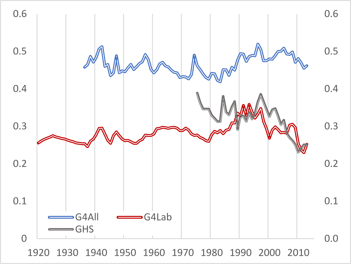
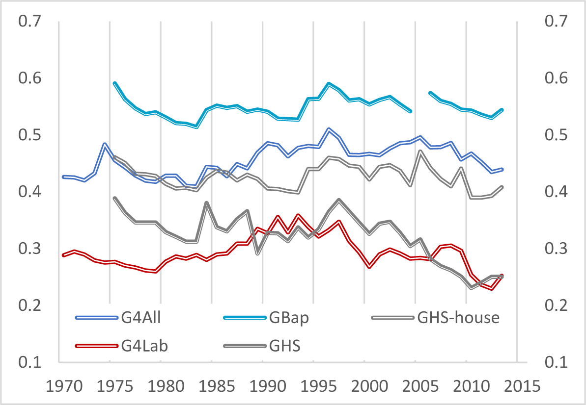
Figure 4 plots their long-run evolution of the overall Gini and the labor Gini alongside the official household-survey Gini (GHS),Footnote 14 which serves as an external benchmark for comparison. The close correspondence between G4Lab and GHS during overlapping years provides reassurance regarding the ability of the occupational approach to capture broad inequality trends.
Income inequality in Venezuela.

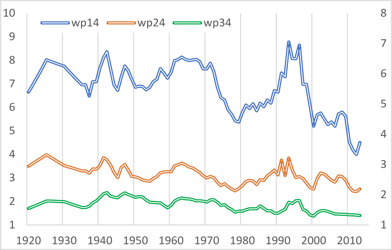
Two main results emerge from Figure 4. First, because capital income is highly concentrated in Group 1, movements in overall inequality closely track those of functional inequality – with a simple correlation of 0.87. Accordingly, the trajectory of G4All is primarily shaped by the relative evolution of aggregate capital and labor incomes and by the operation of the fiscal, structural, and wealth channels. Second, trajectories in labor inequality reflect changes in skill-related wage differentials across occupational groups and the action of the first two channels. In particular, movements in the labor Gini are largely driven by variations in the skill premiums, measured as the ratio of average remuneration of Groups 1–3 relative to Group 4 (Figure A3). Trends in these premiums between 1975 and 2003 closely mirror those reported by Ortega and Pritchett (Reference Ortega, Pritchett, Ricardo Hausmann and Rodríguez2014) for primary, secondary, and tertiary education.
Divergent movements in G4All and G4Lab indicate that the distributive effects of wage premiums are largely offset by changes in the capital share, whereas parallel movements suggest that the allocation of capital income either reinforces, or does not materially alter, labor-income inequality. For any given level of capital income, different configurations of premiums – whether driven by rising unskilled wages or increasing skilled wages – can therefore generate similar levels of total labor income and capital shares.
Figure 4 identifies three decades characterized by distinct inequality dynamics – the 1960s, 1970s, and 2000s – while the remaining decades display broadly coincident movements in both occupational Ginis. To clarify the role of the three channels, the transmission mechanisms, and mediating factors outlined in Section 3, the discussion is organized around Period 1 and Period 2, with particular attention to decades exhibiting contrasting trajectories, which provide additional analytical leverage.
5.1. Period 1: 1920–1973
The factor-income backdrop during this period was marked by a steady rise in real national income, particularly in remunerations per worker across all four occupational groups, with an acceleration after 1950 (Figure A4). Through the fiscal channel, real oil revenues increased steadily up to around 1960–interrupted by a temporary decline during the Second World War – before entering a sustained downturn in the 1960s, driven by falling real oil prices and rapid population growth.
For the years 1920–1935, the absence of national income data precludes direct estimation of overall inequality. To approximate labor-income inequality, I rely on evidence from central government remunerations in 1920, 1925, 1930, and 1935 (Carrillo Batalla, Reference Carrillo Batalla2003). Although public employment remains limited,Footnote 15 average remunerations by occupational category closely match mean incomes recorded in the 1936 economic census, making skill premia a reasonable proxy for economy-wide trends (OA.2). These estimates suggest broadly stable labor inequality, with 1935 levels similar to those in 1920, consistent with stagnant real wages and a stable wage structure until the mid-1930s (Valecillos, Reference Valecillos2007, p. 103).
Between 1936 and 1949, inequality rose sharply as a result of the Second World War, indicating that this major external shock disproportionately reduced labor incomes at the bottom of the distribution, amid a contraction in economic activity and a temporary decline in oil revenues in the early 1940s.
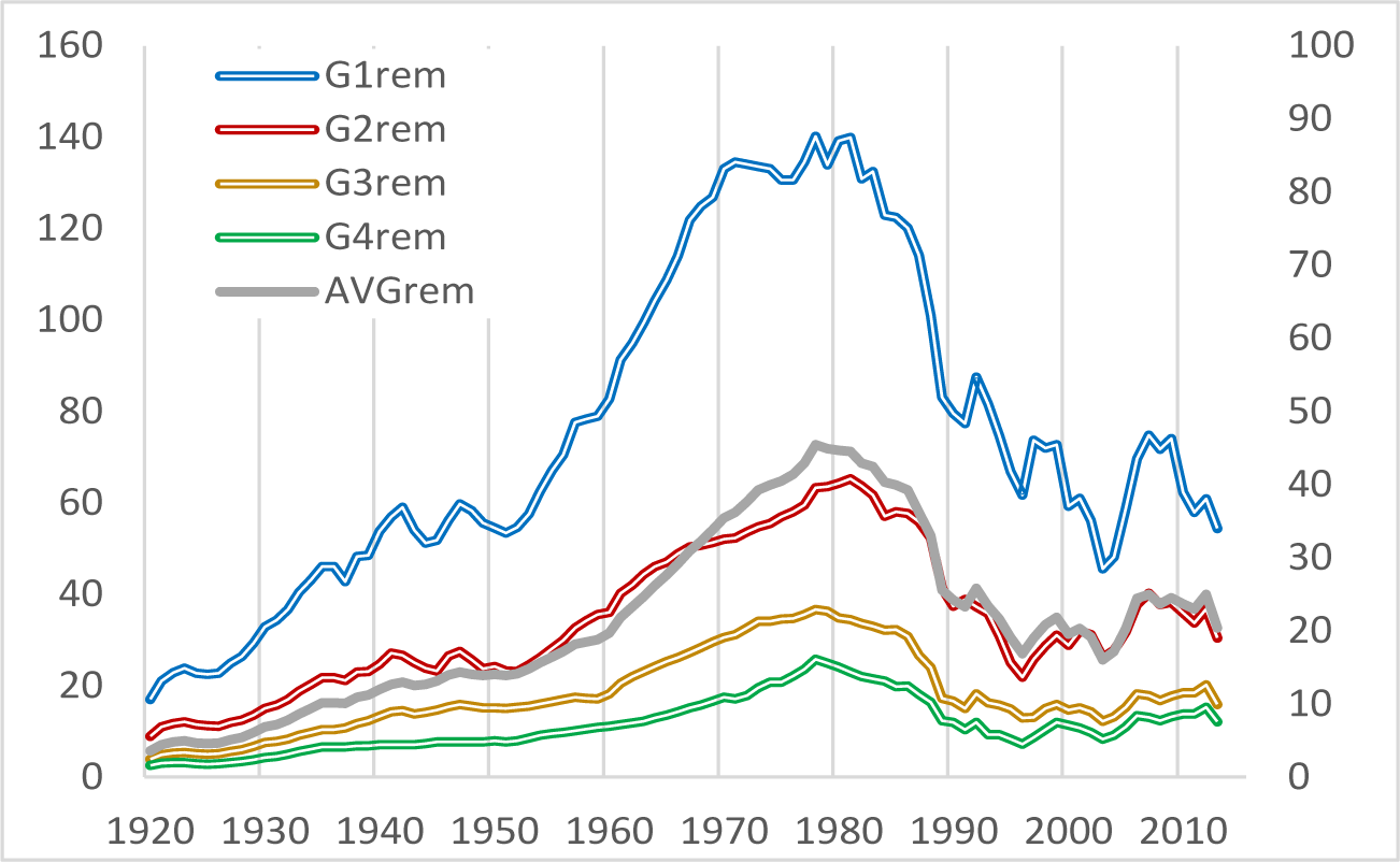
The 1950s and 1960s display contrasting dynamics. During the 1950s, overall inequality widened alongside expanding public expenditure and rapid non-oil growth – particularly in manufacturing and construction – which disproportionately boosted profits and their concentration, reinforcing the disequalizing impact through the wealth channel.Footnote 16 Conversely, inequality narrowed in the 1960s, as declining real oil revenues constrained public spending and slowed non-oil expansion. This compressed capital income per worker, while real wages continued to rise (Figure 3). The sustained growth of labor incomes across both decades reflects the consolidation of a growing urban middle class, supported by rising educational attainment and urbanization (Valecillos, Reference Valecillos2007).
After widening in the 1950s, labor inequality remained broadly stable during the 1960s. Rising wage premiums in the earlier decade reflected skilled-labor shortages combined with strong demand generated by industrialization. Their subsequent stabilization is consistent with expanding skill supply and the absorption of surplus labor into higher-productivity sectors, in line with the Kuznets–Lewis mechanism.
5.2. Period 2: 1974–2013
Relative to Period 1, the second phase exhibits alternating inequality trends amid a sustained decline in real national income from 1978 to 2000, followed by a modest recovery in the 2000s. Crucially, in this period, episodes of widening inequality coincided closely with sharp falls in real wages.
After the 1973 price shock, overall inequality was higher on average throughout much of the decade, peaking around 1974–1975. This was driven by expansionary fiscal policy and large-scale public investment, which boosted profits in construction and protected manufacturing sectors that held significant market power. Employment – especially in the public sector – and the wage bill also expanded. However, capital income rose more than proportionately relative to labor income, widening inequality, before returning to pre-boom levels by the end of the decade as aggregate remunerations accelerated.
Despite rising overall inequality, labor inequality declined, a trend corroborated by the household-survey Gini. This reflects the narrowing of sectoral income gaps following decades of rapid internal migration (Section 3). Gains for the bottom two groups were reinforced by strong unions and the introduction of minimum wages in 1974, which raised the wage floor and strengthened bargaining power among lower-income workers. These equalizing forces outweighed upward pressures stemming from widening educational disparities associated with the tertiary bias in public spending.
Inequality reversed sharply in the 1980s and 1990s, driven by a confluence of forces triggered by fiscal contraction. Physical investment had been declining since the late 1970s (Figure A1), depressing economic activity and labor demand: real private investment fell by 80% between 1978 and 1986, with its share of GDP declining from 29% to 8%. At the same time, delayed demographic effects increased the supply of better-educated workers, while union power eroded rapidly and the real minimum wage collapsed, gradually undoing the wage compression observed during the mid-1970s and pushing skill premia upward. These dynamics, compounded by the debt crisis, the post-1985 oil-price slump, and the neoliberal reforms of 1989, drove a sustained widening of both overall and labor income inequality.
Rodríguez (Reference Rodríguez and Cornia2004) attributes the rise in functional inequality between the early 1980s and 1997 – a trend reflected in overall inequality – to a sustained decline in the capital-labor ratio, which increased returns to capital relative to labor and amplified the inequality effects transmitted through the wealth channel. In a standard growth framework, the distributive impact depends on the elasticity of substitution between factors. Evidence from this period – a rising capital share combined with collapsing real labor income (Figure 3), amid structural rigidities and weak diversification – points to a very low elasticity. As a result, wage adjustments proved insufficient to reallocate labor, contributing to rising unemployment and expanding informality. This outcome is typical of deindustrialization that displaces labor into low-productivity activities.
The oil bonanza of 2002–2013 fueled substantial fiscal expansion, supporting a rebound in real remunerations (particularly in the public sector) and non-oil GDP. Overall inequality widened through much of the 2000s, as capital income again grew more rapidly than labor income, alongside persistent wage premiums for Group 1. By contrast, the underlying trend in G4Lab experienced a fall in the middle of that decade, reflecting declines in premiums for Groups 2 and 3 that were supported by the recovery of the real minimum wage (Mateo Tomé, Reference Mateo Tomé2010). In the early 2010s, both occupational Ginis narrowed, reflecting a rising labor share and declining wage premiums, driven by falling real wages in Group 1 and gains among Group 4.
5.3. Coda: micro evidence from manufacturing
Micro evidence from industrial surveys provides complementary insights into the dynamics of industrialization and its subsequent reversal (Astorga, Reference Astorga2025). Manufacturing is of particular analytical interest because it is highly prone to skill-biased technological change and is predominantly urban and formal, thereby minimizing the direct distributional effects of labor-market segmentation. Between 1953 and the early 1970s, white-collar wage premiums (a basic indicator of wage inequality) rose alongside expanding white-collar employment shares, consistent with persistent skill shortages and the diffusion of skill-biased technological change. From around 1974, however, premiums began to decline while white-collar employment shares continued to expand until the mid-1980s, reflecting the combined effects of easing skill constraints, strengthening unions, and institutional wage compression. This pattern is consistent with the contemporaneous narrowing of labor income inequality at the economy-wide level. The decline in white-collar premiums continued into the early 1990s (no data separating salaries and wages are available thereafter), despite labor shedding. This suggests that those blue-collar workers who remained employed were largely insulated from the downward wage pressures associated with the expansion of informality elsewhere in the non-oil economy, reinforcing the central role of labor-market institutions in mediating distributional outcomes.
To assess the robustness of these results, the next subsection compares the occupational Ginis with alternative inequality series derived from household surveys and national accounts.
5.4. Comparisons with alternative Ginis
For Period 2, it is possible to compare my occupational Ginis with several alternative inequality series as shown in Figure 5.
Alternative Ginis.

Figure 5. Long description
The multi-line graph compares various Gini indices from 1970 to 2015. The horizontal axis represents years, while the vertical axis shows the Gini coefficient, an inequality measure, ranging from 0.1 to 0.7. Five lines are plotted: G4All (overall Gini), G4Lab (labour Gini for four groups), GBap (Gini from Baptista and Vallez), GHS (Ginis based on household surveys using people employed) and GHS-house (Gini based on household surveys using households). The G4All line fluctuates between approximately 0.5 and 0.6, showing a gradual decline after 2008. The G4Lab line ranges from about 0.3 to 0.4, with notable peaks in the mid-1990s. The GBap line varies between 0.4 and 0.5, showing a slight decrease over time. The GHS line is similar to GHS-house, both moving between 0.3 and 0.4, with convergence around 2010. G4All is consistently the highest measure, while GHS-house shows relative stability. The graph illustrates changes in inequality, highlighting the differences between overall, labour and household-based measures. Visual differentiation includes solid and dashed lines, aiding in distinguishing each series.
First, I compare my overall Gini (G4All) with those estimated by Baptista (Reference Baptista and Giordani2006b) for 1975–2004 and by Vallez (Reference Vallez2018) for 2005–2014. These authors derive capital income residually from the national accounts – as the difference between national disposable income and total labor remunerations – and allocate it across households according to the distribution of labor income observed in household surveys.
As a result, movements in their series (GBap) tend to mirror those of the household-survey Gini (GHS-house), and, to a lesser extent, the official GHS. Despite methodological and data differences, the trajectories of G4All and GBap are broadly aligned between 1975 and 1987 and again after 1993. The discrepancies observed between 1988 and 1991 largely reflect divergent movements in labor inequality.
A second comparison of interest is between G4Lab and the GHS. During the critical years 1974–1979, both measures display a clear decline, confirming the strongly equalizing effect of the 1970s oil boom via wage compression. However, while G4Lab turns upward from 1980, the GHS continues to fall until 1983. From 1984 to the mid-1990s, all three measures exhibit rising trends, and they again move in tandem during the 2000s, when inequality declines.
Finally, several point estimates for specific years provide additional evidence on short-term trends. The decline in overall inequality during the 1960s is consistent with Urdaneta’s (Cuadro III-23) estimates of personal income concentration for 1960 and 1967, incorporating data on tax returns and the size distribution of bank accounts. She found that the top 12.1% of the labor force received 53% of total income in 1960, whereas the top 16.4% received 51.7% in 1967, indicating a reduction in concentration. Similarly, the shift from relatively low inequality in the mid-1960s to higher levels following the 1973 oil shock is consistent with Musgrove’s (Reference Musgrove1981, Table 3) estimates based on HBSs – which include capital income – conducted in Caracas in 1966 and 1975. The individual Gini rose from 0.451 to 0.489, while the income share of the top decile increased from 31.5% to 37.1%. Fernández Bujanda et al. (Reference Fernández Bujanda, Torres, de Ferrán L and Vargas2008), using comparable HBSs for 1997 and 2005 covering capital income, report a decline in the Gini from 0.487 to 0.457. Although this fall conflicts with the trajectory of G4All, which records broadly stable inequality over this period, it is consistent with the downward movement observed in G4Lab.
5.5. Distributional impact of in-kind social transfers
So far, the analysis has focused on primary (pre-transfer) income inequality, abstracting from the distributive role of social transfers. This is a significant omission in Venezuela, where such transfers were largely financed by oil fiscal revenues. In this section, I incorporate the distributional impact of in-kind transfers in education and health to construct an extended income measure of inequality.Footnote 17 Although government revenues are not formally earmarked, STinK are treated as oil-funded given the dominance of oil revenues in total fiscal revenues (Figure A1).
A secondary, albeit distinct, form of in-kind benefit is the petrol subsidy, as domestic fuel prices have remained far below international levels since the mid-twentieth century. However, as this implicit subsidy reflects foregone export revenues rather than recorded fiscal outlays, it is not captured in the national-accounts framework used here and is therefore excluded from the extended income measure. Estimates suggest that it amounted to around 3–6% of GDP in the late 2000s and early 2010s (Mendoza, Reference Mendoza2014), with benefits accruing disproportionately to higher-income households and firms.
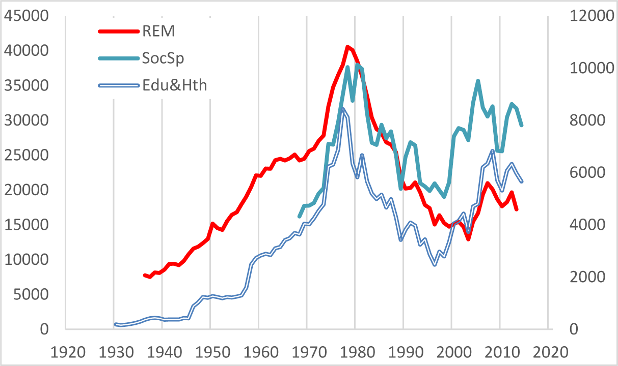
As noted in Section 3, oil-rent-driven public spending was strongly pro-cyclical. Crucially, social spending in 1968–2013 tracked trajectory changes in remunerations (Figure A6); using remunerations as a comparator is more meaningful than GDP, as social policy should be evaluated against the income it is intended to replace or stabilize. Ultimately, this pro-cyclicality constrained the government’s ability to use social transfers to compensate for recurrent collapses in labor income. In Period 1, public spending on education and health (and likely total social spending) grew alongside oil rents as part of a general economic expansion; because external shocks were relatively minor, the state was rarely required to cushion a fall. However, in Period 2, the state ceased to act as a stabilizer and became a volatility transmitter. When rents dropped between 1983 and the late 1990s, instead of maintaining social spending to protect the poor during the recession (a counter-cyclical response), the government slashed expenditure to prevent fiscal collapse.
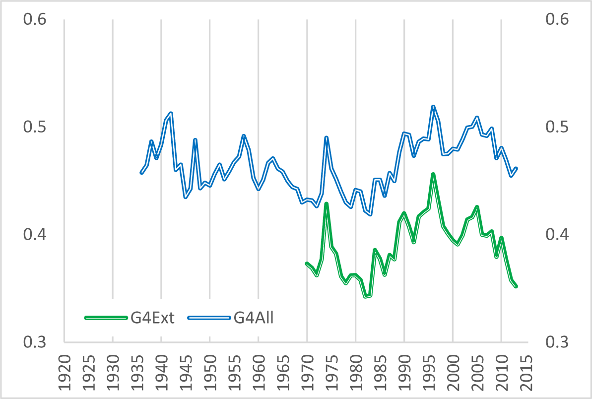
For a given amount of in-kind social transfers, the question arises of how to allocate them across the four occupational groups, assuming that the economically engaged are the recipients. To address this issue, I rely on the fiscal-incidence analysis of Seijas et al. (Reference Seijas, Moreno and González2003) using data from the 1997 HBS to estimate extended-income inequality between 1970 and 2013, as shown in Figure 6.
Extended Gini.

Away from the 1997 benchmark, changes in group size and aggregate transfers are accounted for, but the proportional allocation observed in 1997 is held constant (OA.3). This assumption may introduce distortions when comparing G4Ext across decades with distinct structural and distributional characteristics. After a decline in real social spending per capita between the mid‑1980s and late 1990s, expenditure expanded significantly under President Chávez, driven by large-scale transfers through the misiones sociales,Footnote 18 surpassing the levels observed in the 1970s. Since the main beneficiaries of these programs were those at the bottom of the income distribution (De Luca et al., Reference De Luca, Seiffer and Kornblihtt2013), the progressivity of STiK during this period is likely to have increased relative to 1997, which means that G4Ext underestimates the fall in income inequality.
Two clear patterns emerge from Figure 6. First, in‑kind transfers substantially reduce inequality, although the magnitude varies: 15.8% in 1975, 16.3% in 1985, 14.6% in 1997, and 18.9% in 2007. Second, the trajectories of G4All are broadly robust to the inclusion of transfers, indicating that underlying distributional trends are not driven by public service provision, consistent with its strong pro-cyclicality. However, G4Ext displays more pronounced declines between 1998–2001 and 2005–2010. Finally, while this section focuses on in-kind transfers, a complementary gross calculation (not shown) indicates that the inclusion of direct cash transfers could represent, on average, a further reduction in inequality of between 3 and 5 percentage points, without significantly altering the observed trajectories.
6. Conclusions
This paper studies income inequality in Venezuela over the long term, with the aim of clarifying whether oil wealth has served to create a more equitable society or to reinforce long-standing historical disparities. A major obstacle to addressing this question is the scarcity of income data. Standard sources, such as comparable household surveys, begin only in 1974 and cover labor income alone, while historical tax records are very limited. Consequently, the first task was to construct a set of occupational Ginis consistently defined over time.
The methodology and data sources used to construct these measures have limitations such as the relatively narrow sectoral coverage of remuneration series, and the reduced – though well-apportioned – number of occupational groups. There is also insufficient wage data to produce a consistent estimation of within-group inequality across the full period; the analysis therefore relies on between-group Ginis. Available evidence, however, suggests that incorporating the within-group component would raise the level of inequality but would not significantly affect its trajectory.
Several assumptions made during the estimation process may also introduce potential bias. Nevertheless, the resulting inequality trajectories prove robust to variations in the income concept, alternative allocations of capital income across groups, and different splits of high earners. Reassuringly, overall inequality trends closely match alternative Gini estimates available for the 1960s and for the period 1966–1975, while post-1974 labor Gini trajectories are broadly consistent with household survey evidence.
Has oil wealth been a force for income equality in Venezuela over the long term? The short answer is no. Venezuela did not become the “Norway of Latin America”: equitable and prosperous. The longer answer is more complex and requires identifying both distributional achievements and shortcomings, and unpacking the contradictory effects of oil-led development on income distribution.
The first key finding is that income inequality was primarily oil-driven, but there is no simple answer regarding the direction of its influence. Complexity arises from the differing dynamics of capital and labor incomes, as well as the contrasting trajectories across two distinct periods, making conclusions largely contingent on the measure and period considered.
During Period 1, oil revenues were largely determined by production quantities rather than prices. Inequality was influenced by a steady rise in oil output and government spending, which shaped structural transformations. Overall inequality narrowed from the late 1950s, reflecting the consolidation of the middle class, with growth in real remunerations outpacing capital income gains. By contrast, labor inequality initially rose, likely due to skill shortages and a significant labor surplus, although it declined during the 1960s in response to tighter urban labor markets.
Developments in Period 2 were more varied and largely shaped by the dynamics of a rentier economy. Oil revenues now depended primarily on international oil prices rather than on domestic production decisions, making the economy highly vulnerable to external shocks. Consequently, the fiscal channel was transformed from a stabilizer into a volatility transmitter. Venezuela benefited from substantial oil windfalls between 1974 and 1981, and again during the oil boom of the 2000s. By contrast, a market glut in the mid-1980s caused a steep fall in oil prices, which was only partially reversed by the late 1990s. Overall inequality widened during both booms: in the 1970s, a more than proportional rise in capital relative to labor income easily offset falling premiums, while in the 2000s the expansion was driven by a rising capital share. Inequality also increased during the slump, driven by growing premiums. Labor inequality, however, narrowed steadily during the 1970s, as well as in the mid-2000s and early 2010s, but widened during the slump. This pattern suggests that oil price shocks have distributionally asymmetric and non-linear effects on overall inequality, whereas labor inequality exhibits a sign-dependent response.
In-kind social transfers in education and health substantially compressed inequality relative to primary-income levels, particularly for the lowest-income groups, in Period 2. However, their redistributive impact was fundamentally constrained by the pro-cyclical nature of oil-rent-driven fiscal spending. In the absence of effective stabilization mechanisms, the state ceased to act as a buffer and instead functioned as a transmitter of external volatility, particularly following the 1983 crisis. Ultimately, while these transfers provided significant welfare gains during episodes of high oil prices, they offered only a partial and precarious counterbalance to the structural inequality embedded in Venezuela’s oil-dependent economy, failing to shield the most vulnerable when labor incomes collapsed.
The interaction of endogenous structural transformations, external oil shocks, and the 1980s Debt Crisis is crucial for understanding inequality during Period 2. The sustained fall in physical investment post-1978, combined with the oil slump after 1986, depressed economic activity and reduced labor demand – precisely when demographic shifts and educational expansions were increasing the supply of better-educated workers. The relative capital intensity of industry, limited diversification, and rising labor informality, coupled with a rapid erosion of union power, exacerbated inequality. Ultimately, prosperity primarily benefited the top group, while adversity disproportionately affected those at the bottom. Taken together, these results confirm that Venezuela’s inequality dynamics were shaped by the interplay of forces operating through the fiscal, structural, and wealth channels – as identified in the paper’s analytical framework – and were mediated by labor-market rules and property regimes (Figure 1).
This paper reconciles ambiguous findings in the literature on oil price shocks and inequality. While cross-country studies often report mixed effects, and country-specific analyses depend on the inequality measure used, my findings show that these discrepancies reflect distinct, period-dependent distributional channels. By distinguishing between labor and overall income inequality, I show that oil booms and busts can generate qualitatively different – and sometimes offsetting – effects across income components. Focusing exclusively on booms or on a single inequality measure may therefore misrepresent their aggregate distributional impact.
I conclude this paper by considering developments in Venezuela over the past decade under President Maduro. Although outside the core period of analysis, recent developments provide a stark illustration of the long-term dynamics identified in this paper. Economic activity and income generation have suffered an unprecedented collapse, driven by institutional weakening, legal uncertainty, and prolonged socioeconomic crisis Rodríguez (Reference Rodríguez2025). Deepening poverty and political repression have contributed to massive emigration flows: according to the United Nations Refugee Agency, nearly 7.9 million Venezuelans had left the country by late 2025 in search of better living conditions and protection abroad. This exodus has hollowed out the working‑age population, with potential implications for labor shortages and upward pressure on skill premiums. Moreover, low labor force participation and rising dependency ratios may undermine productivity, raise labor costs, and strain already embattled social services.Footnote 19
The publication of official household surveys since 2014 has been sporadic and of limited reliability. In response to this information gap, private institutions have produced the Encuesta Nacional de Condiciones de Vida (ENCOVI), which highlights three fundamental changes in living conditions between 2014 and 2024: a marked rise in inequality (with the Gini coefficient increasing from approximately 0.407 to around 0.539), a very high incidence of poverty affecting roughly 73% of households, and the growing importance of remittances as a source of income.
Under these conditions, many households have become less dependent on government spending and instead rely on remittances and assets abroad. This has contributed to a new divide between, on the one hand, households with access to hard currency and external support, which enjoy higher purchasing power and tend to occupy the upper and middle segments of the distribution, and, on the other hand, those dependent on local labor income and public subsidies. But those at the very top, in all probability, are dominated by high-ranking officials of Maduro’s regime and in the military.
This paper began by treating state ownership of oil as a developmental promise of income equality and shared prosperity. The long‑run evidence instead documents a profound reversal after an initially auspicious start. Despite sustained real wage growth through much of the twentieth century, the post‑1970s period is characterized by rising inequality and declining real wages, irrespective of oil price cycles. The Venezuelan case thus illustrates how public ownership of natural resources, in the absence of durable mechanisms of accountability and equitable redistribution, can transform an egalitarian aspiration into a persistent distributional failure. In this sense, the history examined here is not only retrospective: it helps explain why struggles over the control and distribution of oil revenues continue to shape Venezuela’s economic and social conditions.
Supplementary material
The supplementary material for this article can be found at https://doi.org/10.1017/S0212610926101219.
Acknowledgements
The author is most grateful to Raúl Crespo, Valpy FitzGerald, Leonardo Maldonado, Osmel Manzano, Brian McBeth, José Manuel Puente, and Leonardo Vera for their generous help. Special thanks are due to Lourdes Urdaneta de Ferrán and Héctor Valecillos Toro for their insightful comments and data sharing. Many thanks also to an anonymous referee. Earlier versions of this paper were presented at the Third World Inequality Conference (Paris, June 4–6, 2026); the High Seminar in Economic History (University of Gothenburg, March 11, 2026); the World Economic History Congress (Lund, July 30, 2025); the XIV Congress of the Asociación Española de Historia Económica (Las Palmas, January 21–24, 2025); and the workshop “Desigualdad en Iberoamérica en el largo plazo” (Universitat de València, October 3–4, 2023). Additionally, an AI language model was used to assist with language editing, stylistic streamlining, and drafting support, including the formulation of prose based on arguments and concepts supplied by the author. All data interpretations, structural arguments, and conclusions remain solely those of the author.
Funding statement
This research received financial support from project PID2021-125901NB-I00, funded by MCIN/AEI/10.13039/501100011033/FEDER, UE.
Appendix A: Complementary Figures and Tables
Oil shares of GDP, exports, and fiscal revenues plus GDP per capita.

Figure A1. Long description
Four series from 1920 to 2010: oil percent of GDP, oil percent of exports, oil percent of revenue and GDP per capita. The x-axis represents years from 1920 to 2010. The left y-axis shows proportions from 0.0 to 1.0, while the right y-axis shows GDP per capita in thousands of Bs. at 1984 prices, ranging from 0 to 40. The blue line represents oil percent of GDP, the orange line represents oil percent of exports, the gray line represents oil percent of revenue and the yellow line represents GDP per capita. Key trends include a sharp rise in oil percent of GDP and oil percent of exports around 1950, followed by fluctuations. Oil percent of revenue shows a peak in the mid-20th century and declines towards 2010. GDP per capita shows gradual growth with peaks around 1980 and 2010. The graph highlights the relationship between oil metrics and economic growth over time. Sources: Baptista (2006a) for oil percent of GDP and GDP per capita; Manzano (2014) for oil percent of exports and oil percent of revenue.
Co-movements in key macroeconomic variables.

Figure A2. Long description
The x axis shows years with tick labels 1920, 1930, 1940, 1950, 1960, 1970, 1980, 1990, 2000, 2010. The x axis range is 1920 to 2010. The left y axis shows tick labels 0, 5, 10, 15, 20, 25, 30. The left y axis range is 0 to 30. The right y axis shows tick labels 0, 5, 10, 15, 20, 25, 30. The right y axis range is 0 to 30. Legend labels: GDPnon-oil, PrivConsum, Imports, Expenditure. Text below the graph: All series are in per capita terms at constant 000s Bs. of 1984 prices. Sources: Baptista (2006a) for GDPnon-oil, Private consumption, merchandise Imports; MOxLAD (2025) for Expenditure using the CPI as deflator. GDPnon-oil line: values rise from about 2 in the early 1920s to about 6 by around 1930, then to about 7 by around 1940. Around 1950 the line is about 14. Around 1960 the line is about 17 to 18. Around 1970 the line is about 20. The line reaches a high point around 1978 to 1980 at about 28 to 29, then falls to about 20 by the mid 1980s. From about 1990 to 2000 the line is around 18 to 16. Around 2003 to 2004 the line is about 14 to 15. Around 2010 to 2012 the line is about 21 to 22 and around 2014 it is about 20. PrivConsum line: values rise from about 2 in the early 1920s to about 4 by around 1930, then to about 4 to 5 by around 1940. Around 1950 the line is about 10. Around 1960 the line is about 12 to 13. Around 1970 the line is about 12. The line reaches a high point around 1978 to 1980 at about 21 to 22, then declines to about 16 by the mid 1980s. Around 1990 the line is about 14 to 15. Around 2000 the line is about 12 to 13. Around 2003 to 2004 the line is about 11 to 12. Around 2010 to 2012 the line is about 19 to 21 and around 2014 it is about 18. Imports line: values are near 0 to 1 in the 1920s and 1930s. Around 1950 the line is about 5 to 6. Around 1960 the line is about 4 to 5. Around 1970 the line is about 4. Around 1978 to 1980 the line reaches about 9 to 10, then drops to about 4 to 5 in the early 1980s. Around 1990 the line is about 3 to 4. Around 2000 the line is about 4 to 5. Around 2008 to 2012 the line reaches about 10 to 12, then around 2014 it is about 7. Expenditure line: values are near 0 to 1 in the 1920s and 1930s. Around 1950 the line is about 3. Around 1960 the line is about 6. Around 1970 the line is about 6 to 7. Around 1978 to 1980 the line reaches about 9 to 10, then declines to about 5 to 6 by the late 1980s. Around 1990 to 2000 the line is about 5. Around 2008 to 2012 the line reaches about 11 to 12, then around 2014 it is about 11.
Investment record: 1920–2013.

Figure A3 Long description
Investment in the Private, Public and Oil sectors per capita at 1984 prices, with private investment as a share of GDP plotted on the right axis. The horizontal axis represents years from 1920 to 2010. The left vertical axis shows investment per capita ranging from 0 to 10000, while the right vertical axis shows private investment as a share of GDP ranging from 0.00 to 0.30. The legend identifies four lines: Oil, Public, Private and Private slash GDP. The Oil line is shown in blue, the Public line in orange, the Private line in green and the Private slash GDP line in gray. The Private sector shows a sharp peak around 1979 to 1980, reaching approximately 9000 to 10000 per capita. The Public sector rises mid-century and peaks later. The Oil sector remains comparatively low with smaller peaks. The Private slash GDP line shows a decline over the long run with a notable bump around the late 1970s, peaking at approximately 0.25 to 0.28. The graph highlights differences in investment trends across sectors, emphasizing the significant surge in private investment during the late 1970s.
Average remuneration per worker by groups.

Wage skill premiums.

Figure A5. Long description
The line graph displays three series over time from 1920 to 2020. The horizontal axis represents the years, while the vertical axis on the left shows values in Bs. of 1984 per worker, per year, ranging from 0 to 45000. The vertical axis on the right ranges from 0 to 12000. The red line represents remuneration (REM), the teal line represents social spending (SocSp) and the blue line represents education and health spending (Edu&Hth). The REM line shows a steady increase from 1920, peaking around 2000, followed by a decline. The SocSp line shows fluctuations with peaks around 1980 and 2010. The Edu&Hth line shows a gradual increase over the years. The graph includes annotations about the data sources and calculations used for the series.
Social spending and remuneration per worker.

Figure A6. Long description
Social categories across two periods: 1920-1935 and 1936-2013, with four groups. Each group is characterized by occupations, income and inequality measures. For 1920-1935, columns include Categories, Occupations, Central government, Labor income (wage) and Gini. For 1936-2013, columns include Categories, Occupations, features (divides), Labor income (remuneration), Gini, Overall income and Gini. Group 1: High earners, formal urban roles like fiscal de hacienda and engineers, with income measured by average of 15 observations per five-year period. Group 2: Skilled technicians and administrators, including statisticians and accountants, with similar income measures. Group 3: Urban workers and artisans, such as drivers and nurses, with income measured similarly. Group 4: Rural and unskilled workers, including servants and cooks, with income measured by average of 7 observations per five-year period. In 1936-2013, Group 1 includes professionals in oil and manufacturing, concentrating capital and high wages. Group 2 involves public sector employees and manufacturing blue collars, with some capital. Group 3 consists of blue collars in low productivity sectors, primarily labor. Group 4 includes low-wage agricultural and personal service workers, primarily labor. Gini coefficients indicate inequality, with labels like G4Lcb and G4All representing specific measures. The table highlights a shift from formal urban roles to varied labor definitions over time, with stratification from high earners to low-wage workers.
Occupational groups and income sources

Table A1 Long description
Rows labeled Group 1 through Group 4 pair Spanish occupation examples with a central government employer column, then list labor income notes and a Gini column. A second set of columns lists broader occupation types, a features column labeled features (divides), a labor income column labeled Labor income (remun.), and another Gini column. Final columns summarize overall income and a final Gini column. Group 1 lists occupations including fiscal de hacienda and ingeniero, with central government listed as Ministerios de Hacienda (Finance), Correos (Postal Service) and Sanidad (Health), labor income noted as average of 15 obsevations per lustrum, and blank Gini cells; the broader occupation type is employers, managers, and professionals, features are high earners, largely formal and urban, labor income (remun.) is while collars in oil and manufacturing industries, and overall income is concentrate capital and high wages, with blank Gini cells. Group 2 lists occupations including jefe de estadisticas and cirujano bucal, central government as Hacienda, Correos and Sanidad, labor income as average of 15 obsevations per lustrum, and Gini shown as G4Lab; broader occupation type is technicians and administrators, features are relatively skilled, largely formal, urban, labor income (remun.) is public sector employees, manufacturing blue collars, Gini is G4Lab, and overall income is largely labor and some capital, with the final Gini cell blank. Group 3 lists occupations including motorista and inspector sanitario, central government as Hacienda, Correos and Sanidad, labor income as average of 15 obsevations per lustrum, and blank Gini cells; broader occupation type is urban workers, artisans, features are mixed formal or informal, mostly urban, labor income (remun.) is blue collars in low productivity sectors of food and textiles; obreros in construction, and overall income is primarily labor and limited capital, with blank Gini cells. Group 4 lists occupations sirvientes, lavanderos, and cocineros, central government as Ministerio de Hacienda, Poder Legislativo (the Legislature) and Hospital Militar (Military Hospital), labor income as average of 7 observations per lustrum, and blank Gini cells; broader occupation type is rural and urban unskilled workers, features are largely informal and rural and includes an estimate of subsitance income, labor income (remun.) is low wages in agriculture and personal services; official minimum wages, Gini is G4All, overall income is primarilly labor, and a fraction of capital, and the final Gini is G4All.