


1. Introduction
The year 2016 witnessed a strong reversal in immigration patterns in the United States. While immigration had been strongly increasing relative to the native population, this trend reversed sharply following President Trump’s rise to power, especially for low-skilled workers. Six years later, immigration spiked, recovering sharply. These sharp swings produce considerable effects on welfare, and in this paper, we provide an estimate of the aggregate welfare effects of immigration.
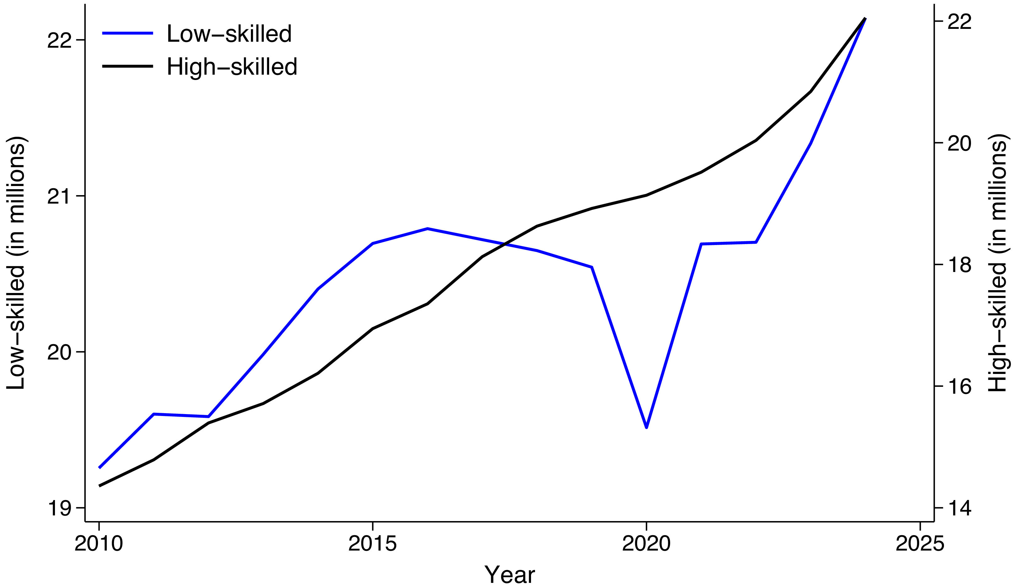
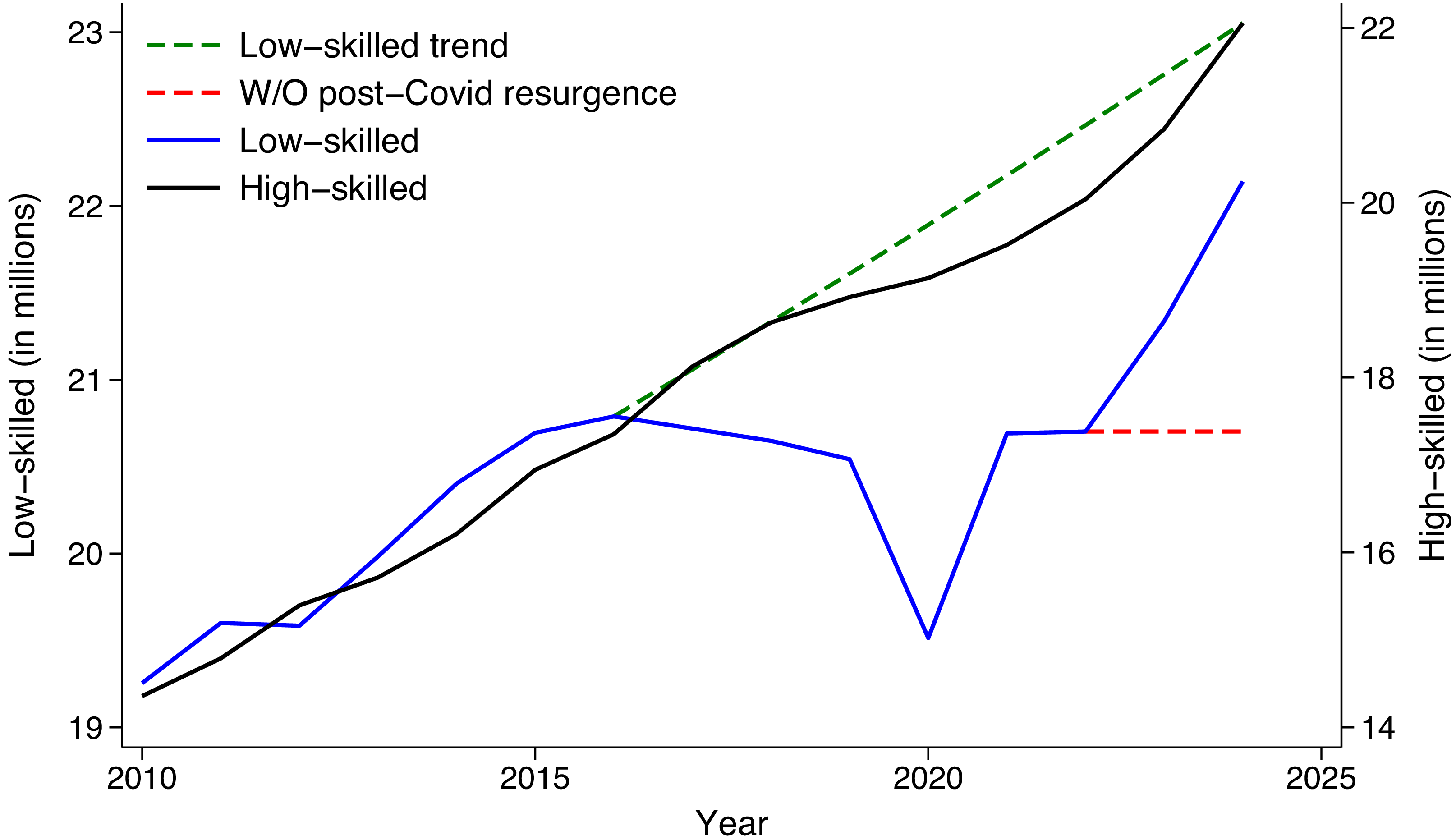
Figure 1 shows the immigration of high- and low-skilled workers. Low-skilled refers to individuals with high school education or less, and high-skilled includes more than high school education. Notice that both in 2016 and in 2022, it is the low-skilled immigrants who are affected. Deviations from the trend among high-skilled are less likely. For this reason, our analysis focuses mostly on low-skilled immigration.
High- and low-skill immigration in the U.S.
Note: Immigration in millions of people. The blue line represents low-skilled immigration (left axis) and the black line represents high-skilled immigration (right axis).

The way immigration affects natives depends on a number of features, such as occupation, industry, education, gender, race, etc. Each characteristic determines the interactions between natives and immigrants; that is, how substitutable they are. By aggregating across these different features, one would learn how immigrants affect the average American. In this paper, we propose to work backward. In the absence of data on the relevant features needed to carry out a deep welfare analysis, we use a micro-founded model to estimate the aggregate. By modeling the “average” complementarity between natives and immigrants, our aim is to approximate the aggregate effects.
Working with the aggregate requires additional considerations relative to a sectoral analysis. The increase in population triggered by immigration has effects on consumption that affect native welfare.
To capture these effects, we build a general equilibrium model with four types of workers: high-skilled natives, high-skilled immigrants, low-skilled natives, and low-skilled immigrants. The model is motivated by the need to account simultaneously for the labor-market interactions between these groups and for the aggregate demand effects of a larger population.
The production side of the model nests the different worker types following Ottaviano and Peri (Reference Ottaviano and Peri2012). High-skilled and low-skilled workers are imperfect substitutes, and within each skill group, natives and immigrants are also imperfect substitutes. This nesting structure allows the model to capture both the complementarity between skill groups and the degree of competition between native and immigrant workers within the same skill group.
To capture the aggregate demand effects of a larger population, we model preferences of the “love for variety” type, building on Dixit and Stiglitz (Reference Dixit and Stiglitz1977). The number of varieties produced is endogenous: a larger workforce supports a greater number of firms and products, which lowers the price of the consumption aggregate and raises welfare. This market-size channel is a key novel element of our framework relative to a standard labor-market analysis.
The welfare estimates depend on three key parameters:
 $(i)$
the elasticity of substitution between domestic and foreign workers of the same skills;
 $(ii)$
the elasticity of substitution between high-skilled and low-skilled workers; and
 $(iii)$
the elasticity of substitution between varieties. Clemens and Lewis (Reference Clemens and Lewis2022) and Brinatti and Morales (Reference Brinatti and Morales2025) argue that the choice of these parameters determines the direction of welfare change from immigration. They show that the strength of the scale effect from additional products relative to the strength of the substitution effect between workers determines the net impact on welfare from immigration. We apply this notion to evaluate the effects of recent immigration swings.
Our headline finding is that the drop in immigration reduces welfare for the average U.S. citizen by 0.3 percentage points of consumption-equivalent units. This aggregate effect is shaped by two distinct channels: the complementarity and substitution channel between worker types and the market-size channel arising from endogenous firm creation. We discuss each in turn.
The gains from immigration are not spread out evenly across the population. High-skilled workers lose more, about 0.5% of consumption units. These gains vary depending on the substitution parameter between high- and low-skilled workers. Considering alternate choices for the parameter, we show that high-skilled natives have higher gains from low-skilled immigration when the elasticity of substitution between skill groups is low. That is, the more the complementarity, the larger the losses from less low-skilled immigrants.
Similar complementarity arguments show that low-skilled workers see increases in their wages when low-skilled immigrants leave. This is because native and immigrant low-skilled workers are relative substitutes.
The market effect worsens for both high- and low-skilled workers, which implies that high-skilled natives are unambigously worse off, given that both channels go in the same direction.
Immigration increases the number of consumers, and in Dixit and Stiglitz (Reference Dixit and Stiglitz1977) models, larger populations can lead to welfare increases. Given preferences featuring “love for variety,” the price of a unit of consumption depends on how many intermediate goods are used to produce the consumption good. The more varieties of intermediate goods, the lower the price of the final consumption good. There is ample empirical evidence that supports the relationship between immigration and firm creation. Orrenius et al. (Reference Orrenius, Zavodny and Abraham2020) study 160 U.S. Core-Based Statistical Areas between 1997 and 2013 and find more immigrants increase the number of firms. Similarly, Olney (Reference Olney2013) finds that increasing the share of low-skilled immigrants by 10% in the 30 largest U.S. metropolitan cities between 1998 and 2008 resulted in a 2% increase in the number of firms. Dustmann and Glitz (Reference Dustmann and Glitz2015) find firm entry accounts for almost 15% of immigrant absorption in the tradable sector in Germany. Beerli et al. (Reference Beerli, Ruffner, Siegenthaler and Peri2021) study Swiss firms following an immigration reform, and find that the reform boosted firm expansion and increased high-skilled native wages by 5% through job creation. Altındağ et al. (Reference Altındağ, Bakış and Rozo2020) study Syrian migrants in Turkey and find that the influx of Syrian refugees increased the number of firms in the Turkish informal sector. In the U.S. context, Mahajan (Reference Mahajan2024) studies the time period 1980–2010 and finds a positive impact of immigration on firm counts within local industries.Footnote 1
We extend the benchmark model to multiple sectors that aggregate via a Cobb-Douglass function into the final consumption good, where sectors differ in how intensive they are in low-skilled immigrants. We compare a two-sector economy to our baseline, with the low-skilled immigrant-intensive sector mapped to the construction sector in the data. Introducing this second sector amplifies the losses from immigration. This is because adding a sector introduces a margin of adjustment of the economy that makes one unit of low-skilled immigrant labor more productive. We map this low-skilled immigrant-intensive sector to the construction sector. Quantitatively the results are very close to the baseline, primarily because of the small share of construction in GDP.
The results in this paper are related to the effects of immigration via complementarities and market size. There are other potential sources of welfare effects that we abstract from. Birinci et al. (Reference Birinci, Leibovici and See2025) show that differences across immigrants other than skill matter: gender, age, time in the country, and country of origin are important. Cortés and Tessada (Reference Cortés and Tessada2011) find effects on market vs. home production. Borjas (Reference Borjas2006) finds effects on internal migration: the inflow of foreigners may impact the location of natives. Howard et al. (Reference Howard, Wang and Zhang2024) find that low-skilled immigration reduces the price of construction. These are effects associated with heterogeneity and are not likely related to market size or worker complementarity.
Several papers link immigration and welfare via the increase in varieties channel. These highlight that inflows of immigrants increase the domestic market size, which results in more varieties in the economy and a higher number of firms in the economy (see Di Giovanni et al., Reference Di Giovanni, Levchenko and Ortega2015; Hong and McLaren, Reference Hong and McLaren2015; Aubry et al., Reference Aubry, Burzyński and Docquier2016; Waugh, Reference Waugh2017, among others). Clemens (Reference Clemens2022) quantify the effects of the reduction in refugee immigration and estimates that the U.S. loses over
 ${\$}$
30,000 per refugee that does not immigrate per year. We contribute to this literature by analyzing the welfare effects of immigration in the U.S., particularly looking at the post-2016 period, where several rigorous immigration policies led to a decline in low-skilled immigrants.
The paper proceeds as follows. Section 2 describes our theoretical model. Section 3 describes the different channels present in the model. Section 4 calibrates the model. Section 5 shows our results. Section 6 expands our model with multiple sectors that differ in low-skilled worker intensity. Section 7 concludes.
2. Model
The theoretical setup features a static closed economy, with a perfectly competitive final goods sector and a monopolistically competitive intermediate goods sector, and four types of labor classified by skill and nativity. Intermediate good producers are heterogeneous in productivity, as in the closed economy in Melitz (Reference Melitz2003).
2.1 Individuals
There are four types of individuals: high-skilled natives, high-skilled immigrants, low-skilled natives, and low-skilled immigrants. Let
 $S_n,S_i,U_n,U_i\ge 0$
represent the mass of each of these types respectively. They all share the same utility function, given by:
 $U = C$
, where
 $C\ge 0$
is consumption of the final good. They maximize utility subject to the budget constraint. Let
 $w_{jk}$
be the wage rate for
 $j=s,u$
and
 $k=n,i$
, where
 $s$
stands for high-skilled labor,
 $u$
low-skilled,
 $n$
is native, and
 $i$
is immigrant. The budget constraint is
 $PC_{jk} = w_{jk}$
, where
 $P$
is the price of the consumption good. Notice that income consists only of wages, that is, there are no profits in this economy. As we mention later, this is because of the free entry condition, which implies no aggregate profits in equilibrium.
2.2 Final good
There is a stand-in firm that produces a consumption good using intermediate good
 $\omega \in \Omega$
, where
 $\omega$
is the name of the good and
 $\Omega$
is the endogenous set containing the names of all goods produced in the economy. The final good producer sells under perfect competition.
The production function follows a CES structure as in Dixit and Stiglitz (Reference Dixit and Stiglitz1977), with elasticity of substitution between intermediates
 $\sigma \gt 1$
,
 \begin{equation} Q=\left [ \int _{\Omega _{}}q_{}(\omega )^{\frac {\sigma -1}{\sigma }}d\omega \right ]^{\frac {\sigma }{\sigma -1}}, \end{equation}
where
 $Q$
is the final consumption good and
 $q(\omega )$
is the quantity of intermediate good
 $\omega$
, for all
 $\omega \in \Omega$
. Let
 $P=\left [ \int _{\Omega }p_{}(\omega )^{1-\sigma }d\omega \right ]^{\frac {1}{1-\sigma }}$
, where
 $p(\omega )$
is the price of the intermediate good
 $\omega$
. The problem of the firm is:
 \begin{equation} \begin{aligned} \underset {\left \{ q(\omega ) \right \}}{\text {max}}\;\;\;\Pi &=PQ-\int _{\Omega }p_{}(\omega )q(\omega )d\omega \end{aligned} \end{equation}
subject to the technology in equation (1). The solution yields demand functions for intermediate goods
 $q(\omega )$
:
 \begin{equation} \begin{aligned} q_{}(\omega )=Q\left [ \frac {p_{}(\omega )}{P_{}} \right ]^{-\sigma }. \end{aligned} \end{equation}
2.3 Intermediate goods
Intermediate goods producers operate in a monopolistically competitive market and use labor as inputs in production. The production function is a CES aggregate of high-skilled and low-skilled labor. The skill demands are further nested into natives and immigrants within skill groups following Ottaviano and Peri (Reference Ottaviano and Peri2012). The production function is
 \begin{equation} q(\omega (\varphi ),A)=A\varphi \left[ \alpha S^{\frac {\eta -1}{\eta }}+(1-\alpha )U^{\frac {\eta -1}{\eta }} \right]^{\frac {\eta }{\eta -1}} , \end{equation}
where
 $A$
is aggregate productivity, common across all intermediate good producers,
 $\varphi$
is firm
 $\omega$
’s idiosyncratic productivity level,
 $\eta$
is the elasticity of substitution between high- and low-skilled labor, and
 $S$
and
 $U$
are skill aggregates of native and immigrant labor defined as:
 \begin{align} S&=\left [\gamma _{s}S_{n}^{\frac {\rho _{s}-1}{\rho _{s}}}+(1-\gamma _{s})S_{i}^{\frac {\rho _{s}-1}{\rho _{s}}} \right ]^{\frac {\rho _{s}}{\rho _{s}-1}}, \text{ and} \end{align}
 \begin{align} U&=\left [\gamma _{u}U_{n}^{\frac {\rho _{u}-1}{\rho _{u}}}+(1-\gamma _{u})U_{i}^{\frac {\rho _{u}-1}{\rho _{u}}} \right ]^{\frac {\rho _{u}}{\rho _{u}-1}}. \end{align}
The parameters
 $\rho _{s}$
and
 $\rho _{u}$
represent the elasticity of substitution between natives and immigrants within the skill groups and
 $\gamma _{s}$
and
 $\gamma _{u}$
capture the average intensity of immigrant labor of either skill type in the production process. The reason for introducing the aggregate productivity parameter
 $A$
is to account for changes outside the model in our empirical application. While the model is static, we obtain our results by calibrating it to all years in the analysis, and allow
 $A$
to change to capture changes outside the scope of the model.
In what follows we drop the name of the good
 $\omega$
and refer to prices as functions of the productivity parameters
 $\varphi$
and
 $A$
, since decisions change only when these parameters change. It is convenient to define the aggregate price index in terms of these variables as follows:
 \begin{align} P(A) = \left [\int _0^\infty p(\varphi ,A)^{1-\sigma }M(A)g(\varphi )d\varphi \right ]^{\frac {1}{1-\sigma }} \end{align}
where
 $p(\varphi ,A)$
solves the maximization problem of each intermediate good producer. These behave monopolistically in their output market, solving the following problem:
 \begin{align} \max _{p,q,l_{sn},l_{si},l_{un},l_{ui}} pq-\sum _{k=sn,si,un,ui} w_k(A)l_k \end{align}
subject to the technology described in equations (4) through (6). The solution to this problem is that price is a constant mark-up over marginal cost. The marginal cost of a type
 $\varphi$
firm is
 $w(A)/\varphi$
, where
 \begin{align} w(A)=&\frac {1}{A}\biggl \{\alpha ^{\eta }\left [\big(\gamma _{s}^{\rho _{s}}w_{sn}(A)^{1-\rho _{s}}+(1-\gamma _{s})^{\rho _{s}}w_{si}(A)^{1-\rho _{s}}\big)^{\frac {1}{1-\rho _{s}}} \right ]^{1-\eta } \notag \\ &+ (1-\alpha )^{\eta }\left [\big(\gamma _{u}^{\rho _{u}}w_{un}(A)^{1-\rho _{u}}+(1-\gamma _{u})^{\rho _{u}}w_{ui}(A)^{1-\rho _{u}}\big)^{\frac {1}{1-\rho _{u}}}\right ]^{1-\eta }\biggr \}^{\frac {1}{1-\eta }} \end{align}
The pricing rule that maximizes profits is to set a constant mark-up, that is,
 \begin{align} p(A,\varphi ) = \frac {\sigma }{\sigma -1}\frac {w(A)}{A\varphi } \end{align}
2.4 Free entry condition
There is an infinite pool of potential entrants. To enter, a potential firm incurs a fixed entry cost of
 $f_{e}$
units of the final good to draw a productivity parameter
 $\varphi$
from a cumulative distribution function (CDF)
 $G(\varphi )$
, with probability distribution function (PDF)
 $g(\varphi )$
. In equilibrium, firms enter the market until the expected profits from entering are equal to the cost of entry, that is,
 \begin{equation} \overline {\pi }[1-G(\varphi ^*(A))]=f_{e}P(A) \end{equation}
where,
 $\overline {\pi }$
is the expected profits before knowing the productivity parameter
 $\varphi$
, that is,
 \begin{align} \overline {\pi }=\int _0^\infty \pi (A,\varphi )g(\varphi )d\varphi \end{align}
where
 $\pi (A,\varphi )$
is the profit of a type
 $\varphi$
firm when the aggregate productivity is
 $A$
.
Equation (11) implies that there are no profits to rebate back to the consumer. This is convenient, given that if this were not the case, we would have to determine how profits are rebated back to the four different types of consumers. Note that this does not prevent firms from making a profit. Net of entry costs, some firms will make positive profits and others negative in a way that aggregate profits are zero.
2.5 Welfare
In equilibrium, consumption (and welfare) is equal to the real wage:
 \begin{equation} C_{jk}(A)=\frac {w_{jk}(A)}{P(A)},\;\;\forall \;\;j=s,u\:;\:k=n,i. \end{equation}
We define aggregate welfare as the sum of individual welfare levels:
 \begin{equation} W(A)=\frac {w_{sn}(A)S_{n}+w_{un}(A)U_{n}+w_{si}(A)S_{i}+w_{ui}(A)U_{i}}{P(A)(S_n+U_n+S_i+U_i)}. \end{equation}
Similarly, native welfare is
 \begin{align} W_n(A) = \frac { w_{sn}(A) S_{n}+w_{un}(A) U_{n}}{P(A)(S_n+U_n)}. \end{align}
3. Equilibrium characterization
Before moving on to the quantitative analysis, we describe the potential mechanisms by which immigration can affect natives’ welfare. In particular, we are interested in how welfare changes from a change in immigration under different parameter values. The most important parameters determining welfare effects are the elasticity of substitution between varieties (
 $\sigma$
), the elasticity of substitution between domestic and foreign workers of a given type (
 $\rho _u$
and
 $\rho _s$
), and the elasticity of substitution between skills (
 $\eta$
). Symmetry implies that changes in
 $\rho _u$
affect low-skilled workers in the same way that
 $\rho _s$
affects high-skilled workers, so we only illustrate how different values of
 $\rho _u$
matter.
For each native type, immigration has two distinct mechanisms that can change welfare: a market effect and a substitution effect. We present figures as aids to our description. All parameters are set to the values described in Section 4 except for our parameters of interest (
 $\rho _u, \eta$
and
 $\sigma$
). We also set
 $\theta = 3.5$
, which is larger than the one we obtained in Section 4. A small value of
 $\theta$
limits the feasible range for
 $\sigma$
, since we require
 $\sigma \lt 1+\theta$
.Footnote
2
Consider first the substitution channel. Low-skilled natives are highly substitutable with low-skilled immigrants, so low-skilled immigrants increase the competition faced by low-skilled natives, lowering their wages. The degree of substitutability is governed by
 $\rho _u$
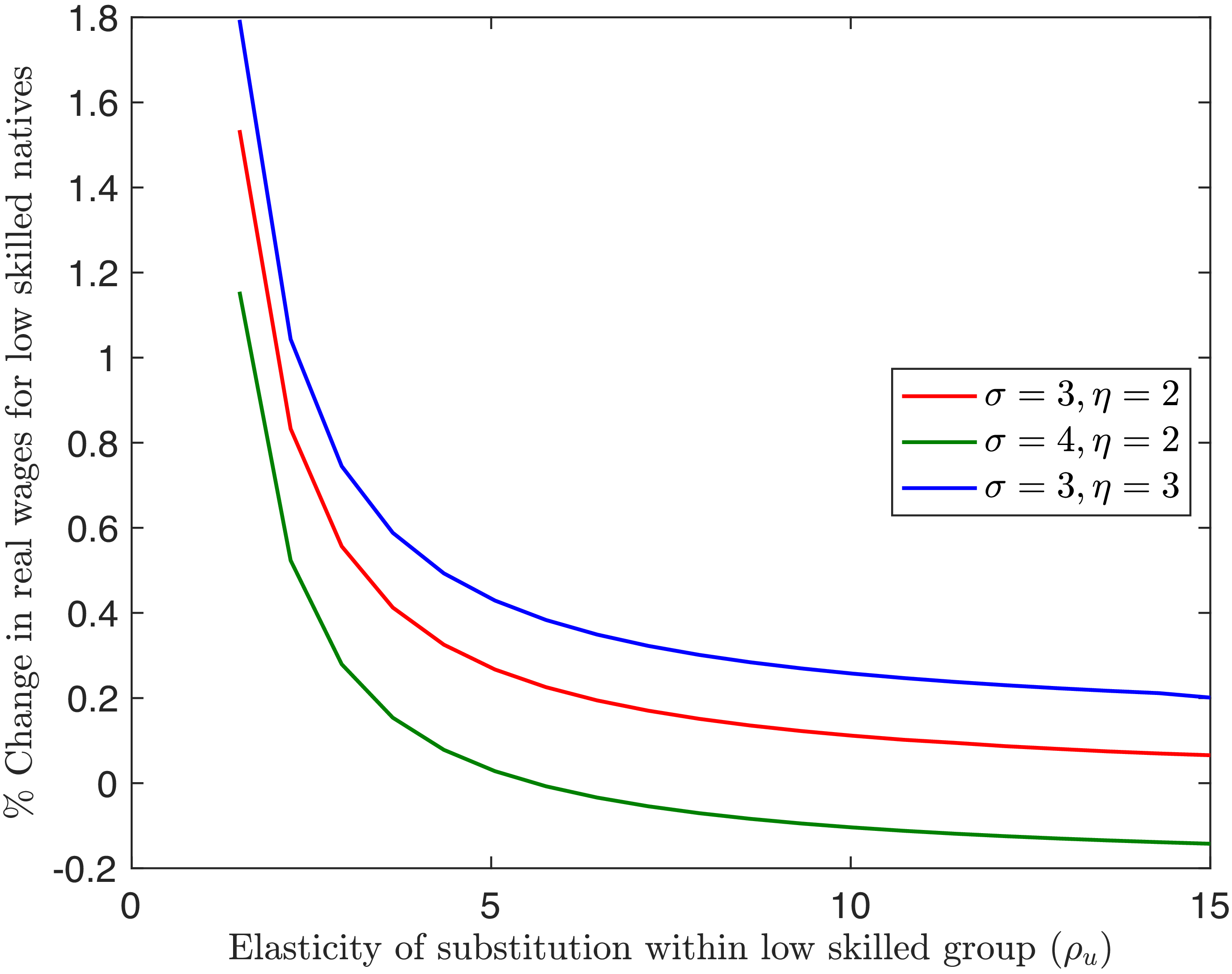
: the larger this is, the stronger the channel. Figure 2 shows how a 10% increase in low-skilled immigrants affects the wages of low-skilled natives under different values of
 $\rho _u$
. As the substitutability between native low-skilled workers and foreign low-skilled workers increases, the gains from immigration drop for domestic low-skilled workers. This is reflected in the fact that the increase in real wages for low-skilled individuals given a 10% increase in low-skilled immigration is decreasing in
 $\rho _u$
(all three lines show this).
Change in low-skilled native wages from a 10% increase in low-skilled immigrants under different parameter values: Substitutability.

Next, consider the complementarity between high-skilled and low-skilled workers. The strength of this complementarity is governed by
 $\eta$
. The smaller this parameter, the higher the complementarity. Figure 2 shows the effect of increasing
 $\eta$
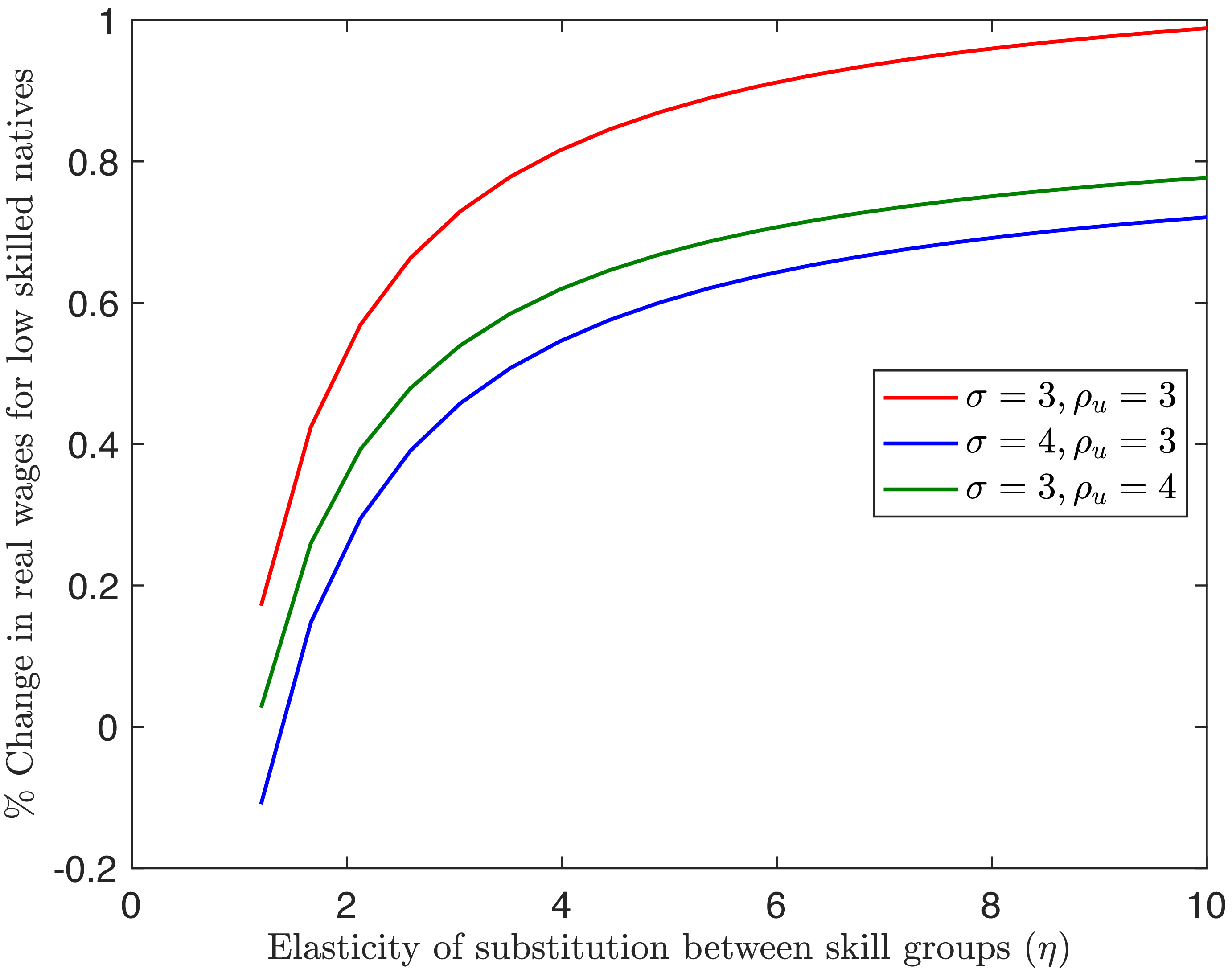
by comparing the red line to the blue line. As we increase the substitutability between workers of different skills, the gains for low-skilled domestic workers increase. This is because, when high-skilled and low-skilled workers are highly substitutable, immigrants compete with both skilled and low-skilled workers, so that labor demand changes will be spread out between skilled and low-skilled. As a result, the drop in demand for low-skilled domestic workers is lower. If this parameter is relatively small, Figure 3 shows that domestic low-skilled workers can lose from an inflow of low-skilled immigrants. The gain in real wages is decreasing in
 $\eta$
, and negative when the complementary channel is strong. This is because when substitution across skill groups is low, low-skilled immigrant workers compete only with low-skilled domestic workers, and the labor demand change accrues to only the low-skilled group.
Lastly, consider the market-size channel. Moving from the red line to the yellow line in Figure 2 shows the effects of increasing
 $\sigma$
: the higher this parameter, the lower the gains for low-skilled domestic labor. The reason is that when
 $\sigma$
is large, goods are easily substitutable among each other. Thus, the gains from varieties drop since one can easily replace across goods. In other words, the degree of increasing returns is decreasing in
 $\sigma$
, so that as
 $\sigma \to \infty$
, this model resorts to a representative firm model, with no increasing returns to scale.
4. Calibration
The discussion in Section 3 shows that domestic workers can gain or lose from immigration, depending on parameter values. This section assumes parameter values consistent with the literature to pin down the actual effect of the changes in 2016 and 2022. By using independent estimates, we provide an unbiased estimate of how welfare is likely to have been affected. More precise results would involve a proper estimation of these parameters, and this is beyond our scope.
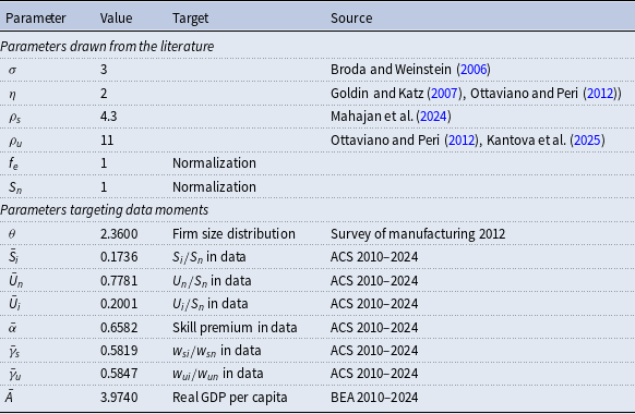
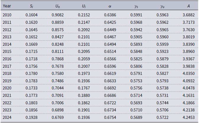
We calibrate the model to the U.S. economy for each one of the years between 2010 and 2024. Our strategy divides our parameters into two sets. The first includes parameters whose value we draw from existing research, and the second set targets data moments. Table 1 reports the calibrated parameters. For parameters that change by year, we report the means and denote this with a bar, that is,
 $\bar x$
denotes the mean of
 $x$
between 2010 and 2024. We report the complete set of parameters in Table A1 in Appendix A.
Calibrated parameters

Table 1. Long description
A table with 12 rows and 4 columns. The columns are labeled Parameter, Value, Target, and Source. The table is divided into two sections: Parameters drawn from the literature and Parameters targeting data moments. The first section includes parameters with values drawn from existing research, and the second section includes parameters calibrated to target data moments. Each row lists a parameter, its value, the target it aims to achieve, and the source of the value. Notable parameters include sigma with a value of 3, eta with a value of 2, and rho sub s with a value of 4.3. The table also includes parameters targeting data moments such as firm size distribution, skill premium, and real GDP per capita.
Note: For the parameters calibrated to target data moments from 2010 through 2024, that includes A,
 $\alpha$
,
 $\gamma _{s}$
,
 $\gamma _{u}$
,
 $S_{i}$
,
 $U_{n}$
,
 $U_{i}$
, Table reports the average of the parameter values over 15 years. The complete set of these parameters for each year is reported in Appendix A, Table A1.
Change in low-skilled native wages from a 10% increase in low-skilled immigrants under different parameter values: Complementarity.

We set the elasticity of substitution between intermediate varieties
 $\sigma$
equal to 3, which lies close to the median estimates by Broda and Weinstein (Reference Broda and Weinstein2006). Following the standards in the literature, we assume that the distribution of productivity is Pareto. This implies that in equilibrium the firm size distribution is Pareto, which closely resembles the upper tail of the firm size distribution in the U.S. (Axtell, Reference Axtell2001). More specifically, we assume
 \begin{align} g(\varphi ) = \theta \varphi ^{-\theta -1}, \ \ \ \varphi \in [1,\infty ), \ \theta \gt 0 \end{align}
We calibrate
 $\theta$
so that our firm size distribution is as close as possible to that in the data. For data, we use the U.S. manufacturing sector for the year 2012 following Rubini (Reference Rubini2014) which gives us a value of
 $\theta$
of 2.36. We obtain this by minimizing the sum of the squared difference between the employee size distribution of manufacturing firms in the data and the model in 2012. The data on the distribution of firms across the employee size bins comes from the 2012 Census of Manufacturing. The Census provides the number of firms hiring less than
 $L_{i}$
workers for a given employment threshold
 $L_{i}$
, where the thresholds are 4, 9, 19, 49, 99, 249, and 499, and the employment bins are denoted as
 $L_{i-1}-L_{i}$
. In the model, we consider
 $L_{i}$
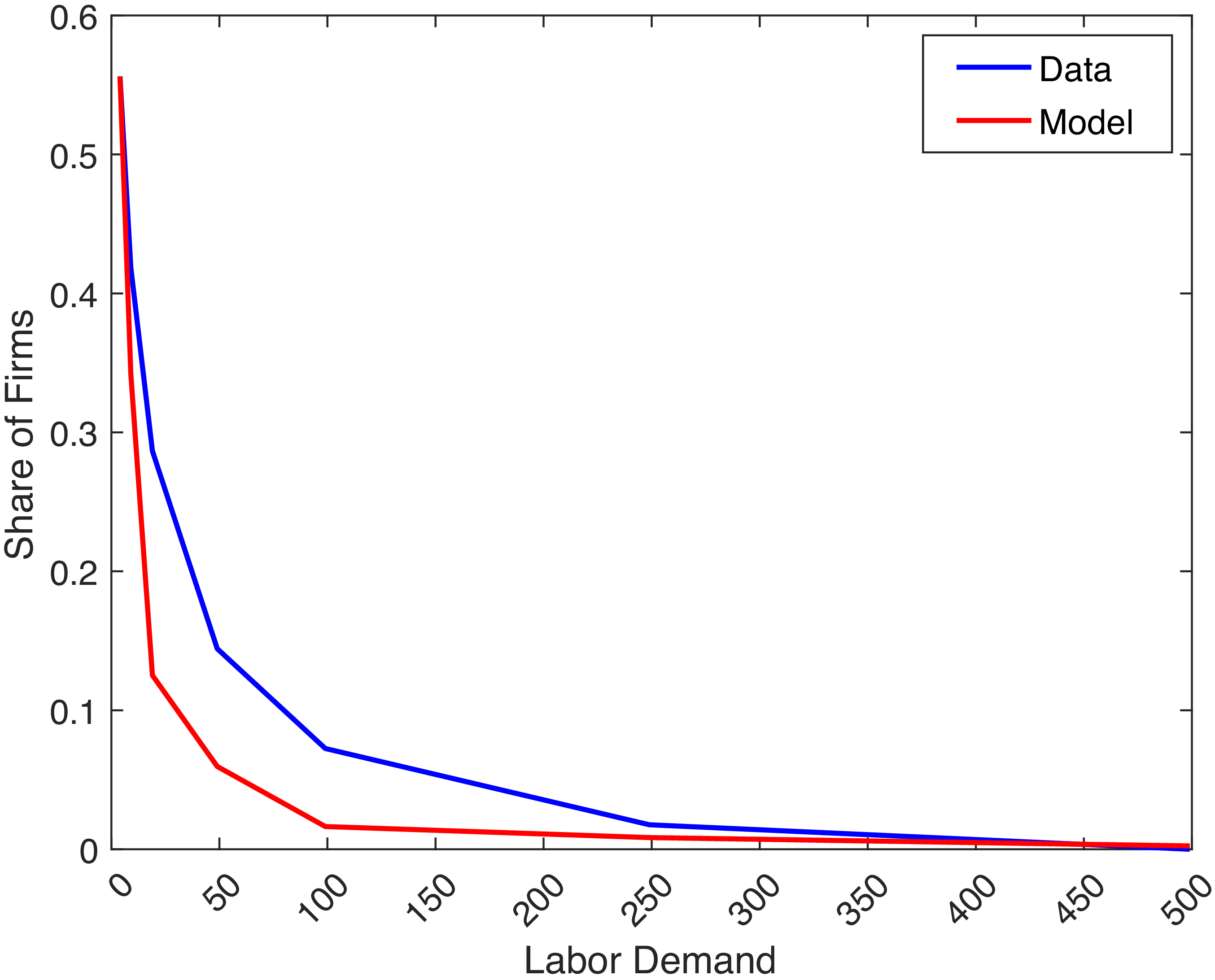
as the summation of the four types of workers for each employment bin. To compare the workers in the model to the workers in the data, we compute the maximum number of workers in each bin with respect to the first bin in the model, such that the share of firms in that bin is the same in the model and in the data. Figure 4 shows the model fit of the firm size distribution observed in the data.
Firm size distribution fit between the model and the data.
Note: The blue line plots the distribution of manufacturing firms across the employment thresholds from the data. The red line plots the distribution generation in the model equilibrium for the year 2012.
Source: 2012 Census of Manufactures.

The fixed entry cost
 $f_{e}$
is normalized to 1. Changing this normalization does not affect our results. The elasticity of substitution between high-skilled and low-skilled labor
 $\eta$
has been extensively studied, with estimates ranging from 1.5 (Katz and Murphy, Reference Katz and Murphy1992; Goldin and Katz, Reference Goldin and Katz2007) to 2.5 (Card and Lemieux, Reference Card and Lemieux2001; Ottaviano and Peri, Reference Ottaviano and Peri2012). We take the mid-point of these estimates and set
 $\eta = 2$
.
The elasticity of substitution between natives and immigrants across skill groups (
 $\rho _{s},\rho _{u}$
) that governs the effect of immigrant influx on the wages is available from the existing literature studying the wage impacts of immigration in the U.S. (Borjas, Reference Borjas2003, Reference Borjas2005; Borjas et al., Reference Borjas, Freeman and Katz2007; Raphael and Smolensky, Reference Raphael and Smolensky2009; Card, Reference Card2009; Ottaviano and Peri, Reference Ottaviano and Peri2012). The elasticity parameter most widely used is around 20, implying imperfect substitution between natives and immigrants when the elasticity is not allowed to vary by skill. Allowing for the substitution parameter to vary by skill, the substitution is higher between natives and immigrants within the high-skilled group which is estimated at around 33, compared to 11.1 for the low-skilled group (Ottaviano and Peri, Reference Ottaviano and Peri2012). Recent studies that focus on firm-level data have estimated elasticities much lower. Mahajan et al. (Reference Mahajan, Morales, Shih, Chen and Brinatti2024) studies college-educated H-1B immigrants and natives and finds an elasticity of substitution of 4.3 between these groups. This number is close to 4.28 as estimated by Brinatti and Morales (Reference Brinatti and Morales2025) for the case of Germany. Thus, we use
 $\rho _s=4.3$
in our calibration. Following Ottaviano and Peri (Reference Ottaviano and Peri2012) and meta-analysis by Kantova et al. (Reference Kantova, Havránek and Havránková2025), we adopt a conservative value of
 $\rho _u=11$
. This value lies between the lower-bound estimates
 $(=5)$
and upper-bound estimates
 $(=20)$
, and reflects substantial but imperfect substitutability between natives and immigrants within low-skilled groups.
Data on labor supply in the U.S. comes from the American Community Survey (ACS) for the years 2010 through 2024. Labor is classified by citizenship as immigrants or natives, and is classified into skill groups of high-skilled (more than schooling) and low-skilled (schooling and less) by years of education. The supply of high-skilled natives
 $S_{n}$
is normalized to 1 for every year, and the labor supply of the other three types of labor
 $S_{i},U_{n},U_{i}$
is calibrated to match their levels relative to high-skilled natives for each year.Footnote
3
The remaining parameters that are calibrated to match the U.S. economy are
 $\alpha$
,
 $\gamma _{s}$
,
 $\gamma _{u}$
, and
 $A$
. These parameters determine the technology in production and how it has changed over the years. The parameter governing the skill share in production
 $\alpha$
is calibrated to match the skill premium in data, that is, the wage ratio between all high-skilled and all low-skilled workers in the US for the years 2010–2024. The parameter governing the share of high-skilled natives in production
 $\gamma _{s}$
is calibrated to match the ratio of high-skilled immigrant wages to high-skilled native wages in the U.S. for the years 2010–2024 and
 $\gamma _{u}$
is calibrated to match the change in the wage ratio between immigrants and natives in the low-skilled group over the years. The common productivity parameter
 $A$
captures other factors that might affect changes in the technological mix in the economy over the years. It is calibrated to match the GDP per capita for the U.S. economy over each year between 2010 and 2024. We use data from the Bureau of Economic Analysis’ (BEA) gross domestic product data series.
5. Results
We present our results in two steps, describing first our analysis of the 2016 immigration reversal, and then focus on the changes in 2022. We conclude this section with an analysis of the expected welfare consequences of policies being considered by the current administration.
Figure 5 shows the level of consumption of all four labor types between 2010 and 2024, normalized to 1 in 2010. It is noteworthy that the low-skilled natives are the ones whose consumption grew the least in this time period, with consumption decreasing from 2015 to 2016. Soon after, this group’s consumption started increasing again, until COVID hit in 2020.
Consumption across labor types (2010–2024).
Note: Parameters targeting data moments vary by year. Variables are normalized to 1 in 2010.

Our counterfactual assumes that low-skilled immigration observed the average growth between 2016 and 2024 that occurred between 2010 and 2016, of 1.3% annually. We represent this in Figure 6 with a green dashed line, while the blue line shows the data.
Immigrant population in the U.S. (2010–2024).
Note: Immigration in millions of people. The blue line represents low-skilled immigration (left axis) and the solid black line represents high-skilled immigration (right axis). The dashed green line represents the low-skilled immigration following the pre-2016 trend (left axis), and the red dashed line represents no growth in low-skilled immigration after 2022. (left axis).

Notice that the behavior of high-skilled immigration is smoother. While it did fall behind trend between 2019 and 2024, it fully recovered by then. Accordingly, our focus is on low-skilled immigration.
5.1 The 2016 immigration reversal
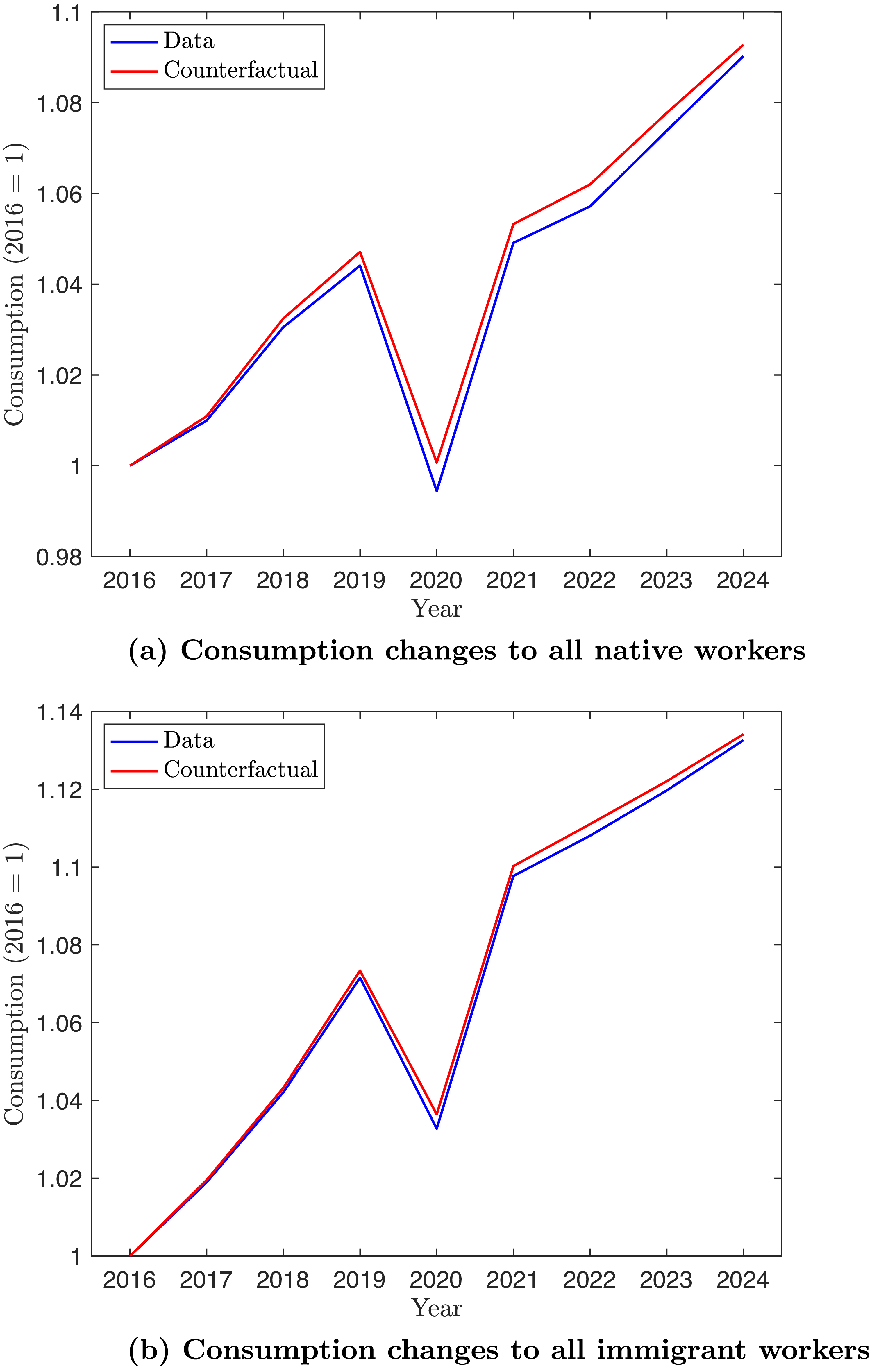
Welfare impacts with counterfactual growth in low-skilled immigrants.
Note: Parameters targeting data moments vary by year. Variables are normalized to 1 in 2016.

Figure 7(a) plots the aggregate welfare for all natives based on equation (15). The blue line shows the change in aggregate welfare over the years based on the actual change in the immigrant population. The red line shows the counterfactual change.
The counterfactual implies higher welfare in every year. Between 2016 and 2019, native consumption would have grown by around 4.6% with a steady annual growth of immigrants of 1.3% in that period, as opposed to an observed growth of 4.3%. As suggested by Figure 3, the substitutability between varieties is key to determine these effects. In Appendix C we show how welfare changes when we increase the value of
 $\sigma$
.
Figure 8 breaks down the effects on natives by skills. There are two lines for the counterfactuals, one corresponding to the lower estimate of
 $\eta$
 $(=1.5)$
, and one to the higher estimates (
 $\eta =2.5$
). We do this because our results for the low-skilled change qualitatively based on this parameter, with mild gains for high values of
 $\eta$
, and mild losses for low values.
Skill complementarity and welfare impacts of counterfactual growth in low-skilled immigrants: Native workers.
Note: Parameters targeting data moments vary by year. Variables are normalized to 1 in 2016.

Figure 8(a) shows the effects for high-skilled workers. The counterfactual shows a considerable increase in welfare, and the increase is roughly the same under both values of
 $\eta$
. Between 2016 and 2019, high-skilled natives would see an average consumption growth of around 5% as opposed to the observed 4.5%, if the immigrant population grew at an annual rate of 1.3%. In 2019 in particular, the welfare of skilled natives would have been 0.5% in consumption-equivalent units larger had immigrants continued on the pre-2016 trend.
Figure 8(b) shows the effects on low-skilled natives. These effects are very mild, hovering around zero. They are slightly positive under high values of
 $\eta$
, and turn slightly negative under low values. Intuitively, the higher the
 $\eta$
, the larger the substitutability between low-skilled immigrants and high-skilled natives. The more substitutable these are, the more they compete in the labor market. Thus, the losses from more competition affect low-skilled natives less, since the effects are more transmittable to high-skilled workers.Footnote
4
One can see this by focusing on the effects on the wage of the native low-skilled in Figure 9. Since immigrants are in direct competition with these workers, the wage relative to the native high-skilled wage drops with immigration. The larger the substitutability with skilled workers, the milder the drop.
Wage effect.
Note: Parameters targeting data moments vary by year. Variables are normalized to 1 in 2016.

The positive effects come from changes in market size. With more workers, the number of varieties produced in equilibrium increases, and this is a source of welfare gains. We show this in Figure 10. The increase in varieties implies a lower cost of the consumption aggregate. Figure 11 shows the effect on the aggregate price level.
Change in mass of varieties.
Note: Parameters targeting data moments vary by year. Variables are normalized to 1 in 2016.

Change in aggregate price.
Note: Parameters targeting data moments vary by year. Variables are normalized to 1 in 2016.

Quantitatively, under the counterfactual, the average native would be able to consume 0.3% more consumption units in 2019 relative to the data. This is a combination of an increase of 0.5% coming from the high-skilled, and no change coming from the low-skilled.
Part of the gains for the high-skilled come from a reduction in the price of the aggregate consumption good, that increases real wages. The low-skilled also benefit from the reduction in the aggregate price level. But the increased competition among this group brings downward pressure on wages. In net, we find that these effects roughly cancel out, so that the counterfactual does not affect the real wages of the native low-skilled.
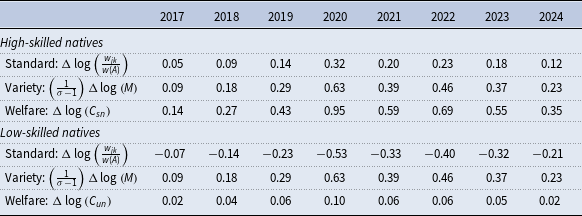
Next, we ask what percentage of these welfare gains or losses arises from ‘standard’ labor market mechanisms that operate through wage changes and how much accrues to increased market size. Using equations (13) and (7), we can decompose the welfare change for high-skilled and low-skilled natives into its components. Specifically,
 \begin{equation} \Delta \;\text {log}(C_{jk})=\underbrace {\Delta \;\text {log}\left ( \frac {w_{jk}}{w(A)} \right )}_{\text {Standard}}+\underbrace {\left ( \frac {1}{\sigma -1} \right )\Delta \;\text {log}(M)}_{\text {Variety}},\;\;\forall \;\;j=s,u\:;\:k=n. \end{equation}
The first component on the right-hand side of equation (17) identifies what proportion of welfare change comes from wage and price changes from the counterfactual increase in low-skilled immigrants. The second component identifies what proportion comes from a change in market size due to the counterfactual. We consider the baseline scenario of
 $\eta =2$
, and compute these components for all the years, which are reported in Table 2. On average, around 33% of welfare gains to high-skilled natives arise from changes in wages and prices. Much of the gains, close to 67%, arise from increased market size from increasing low-skilled immigrants. Since low-skilled natives are directly competing with low-skilled immigrants, the standard component leads to a drop in welfare, which is compensated by the market-size channel.
Components of welfare change (percentage points)

Table 2. Long description
The table presents data on the components of welfare change for high-skilled and low-skilled natives from 2017 to 2024. It has 8 columns representing the years and 6 rows representing the categories and their respective values. The categories are divided into two main groups: High-skilled natives and Low-skilled natives. Each group has three subcategories: Standard, Variety, and Welfare. Row 1: High-skilled natives Standard: 0.05, 0.09, 0.14, 0.32, 0.20, 0.23, 0.18, 0.12. Row 2: High-skilled natives Variety: 0.09, 0.18, 0.29, 0.63, 0.39, 0.46, 0.37, 0.23. Row 3: High-skilled natives Welfare: 0.14, 0.27, 0.43, 0.95, 0.59, 0.69, 0.55, 0.35. Row 4: Low-skilled natives Standard: -0.07, -0.14, -0.23, -0.53, -0.33, -0.40, -0.32, -0.21. Row 5: Low-skilled natives Variety: 0.09, 0.18, 0.29, 0.63, 0.39, 0.46, 0.37, 0.23. Row 6: Low-skilled natives Welfare: 0.02, 0.04, 0.06, 0.10, 0.06, 0.06, 0.05, 0.02.
Notice that the gains from the variety channel depends explicitly on
 $\sigma$
. In fact, increasing
 $\sigma$
considerably reduces the welfare gains. Appendix C shows this. Intuitively, a larger value of
 $\sigma$
reduces the gains from varieties. In the limit as
 $\sigma \to \infty$
, the model becomes one of a representative good, with no gains from variety.
5.2 The 2022 immigration comeback
The declining trends in low-skill immigration that started in 2016 reversed in 2022, when low-skilled immigration sped up, following the relaxation of many restrictions by the Biden Administration. Figure 6 shows these changes. Note that, in spite of the spike, low-skilled immigration is still considerably below the pre- 2016 trend.
Part of this comeback follows the reopening of international travel and visa processing in 2021–2022 related to the travel bans during COVID. There were also efforts by the administration to encourage more immigration. The federal government expanded the cap on H-2B temporary nonagricultural worker visas to address labor shortages in seasonal industries reliant on low-skilled immigrant labor. The termination of Title 42 in May 2023 ended a restriction that limits immigrant entry on public health grounds.
This section asks to what extent did it help natives recover from drops in 2016. Related to this is the question of how different would things be had Biden not lifted some of the restrictions to immigration. Accordingly, our first counterfactual compares the observed welfare levels to those that would have happened had immigration followed its pre-2016 trend. Our second counterfactual “removes” the immigration resurgence between 2022 and 2024. We represent this with a dashed red line in Figure 6.
Figure 12 presents a visual representation of our results. Focusing on high-skilled workers, welfare in 2024 would have been higher by 0.35% consumption units had immigration followed the pre-2016 trend. Notwithstanding, the post-COVID resurgence helped in milding the losses: without it, the high-skilled would be 0.91% worse off in terms of welfare. The effects for low-skilled natives are virtually zero, given the offsetting effects of more competition and more varieties.
5.3 Anti-immigration policies under consideration
We end this section with an analysis of the anti-immigration policies the Trump Administration is currently enforcing. The Deportation Data Project (Hausman, Reference Hausman2025), suggests that the second Trump Administration has deported around 1.5 million low-skilled immigrants.Footnote 5 Similarly, the Department of Homeland Security reports 3 million low-skilled immigrants deported.Footnote 6
We compute welfare changes for high-skilled and low-skilled natives with a 1.5 million drop and a 3 million drop in the low-skilled immigrant population using our calibration for 2024. Table 3 reports the welfare change for high-skilled and low-skilled natives for the corresponding deportation numbers of low-skilled immigrants. With twice the number of deportations, the loss in welfare doubles. High-skilled natives again have a higher welfare loss compared to low-skilled natives.
Change in welfare with approximate deportations in 2025

Table 3. Long description
A table comparing welfare changes for high-skilled and low-skilled natives with deportations in 2025. The table has two columns and two rows of data. Column headers are High-skilled natives and Low-skilled natives. Row labels are 1.5 million deportations and 3 million deportations. Row 1: High-skilled natives, 0.58 percent; Low-skilled natives, 0.04 percent. Row 2: High-skilled natives, 1.16 percent; Low-skilled natives, 0.08 percent.
Welfare changes post-Covid.
Note: Parameters targeting data moments vary by year. Variables are normalized to 1 in 2016.

Figure 12. Long description
Panel A: A line graph shows consumption changes for high-skilled native workers from 2016 to 2024. The x-axis represents the year, and the y-axis represents consumption normalized to 1 in 2016. Three lines are plotted: the observed trend (black), the pre-2016 trend (red), and the trend without the post-Covid surge (blue dashed). The graph shows an initial increase in consumption until 2019, a dip in 2020, followed by a sharp rise and then a steady increase until 2024. Panel B: Another line graph illustrates consumption changes for low-skilled native workers over the same period. The axes and lines are similarly labeled. This graph also shows an initial increase, a dip in 2020, and a subsequent rise, with the observed trend closely following the pre-2016 trend and diverging from the trend without the post-Covid surge.
6. A two-sector economy
This section expands our benchmark model by introducing a second sector that is more intensive in low-skilled workers. We do this to explore how sectoral heterogeneity affects our results.
There are two intermediate goods sectors operating independently in a perfectly competitive market. A representative final goods sector aggregates these sectoral composites via a Cobb-Douglas technology.
 \begin{equation} Q \;=\; Q_1^{\beta }\, Q_2^{1-\beta }, \qquad \beta \in (0,1). \end{equation}
Each sectoral composite
 $Q_m, m\in \{1,2\}$
is a CES aggregate of a continuum of intermediate varieties
 $\omega \in \Omega _m$
:
 \begin{equation} Q_m \;=\; \left [\int _{\Omega _m} q_m(\omega )^{\frac {\sigma _m-1}{\sigma _m}} \, d\omega \right ]^{\frac {\sigma _m}{\sigma _m-1}}, \qquad \sigma _m\gt 1. \end{equation}
Cost minimization by the final-good firm gives the demand for each sectoral aggregate as
 \begin{align} Q_1 \;=&\; Q \left ( \frac {\beta }{1-\beta } \right )^{1-\beta } \left (\frac {P_{2}}{P_{1}}\right )^{1-\beta }, \end{align}
 \begin{align} Q_2 \;=&\; Q \left ( \frac {\beta }{1-\beta } \right )^{-\beta } \left (\frac {P_{2}}{P_{1}}\right )^{-\beta } \end{align}
where the sectoral price indices are
 $P_m = \left [\int _{\Omega _m} p_m(\omega )^{1-\sigma _m}\, d\omega \right ]^{\frac {1}{1-\sigma _m}}$
, for
 $ m=1,2$
. This implies constant expenditure shares for each sector,
 $E_m \;=\; \lambda _m \, P Q$
, where
 $\lambda _1=\beta ,\ \lambda _2=1-\beta$
, and the economy-wide price index
 $P$
is given as,
 \begin{align} P &\;=\; \left (\frac {P_1}{\beta }\right )^\beta \left (\frac {P_2}{1-\beta }\right )^{1-\beta } \end{align}
Similar to the one-sector setup, the intermediate varieties are produced using CES technology in each sector, where a firm with draw
 $\phi _{m}$
and sectoral productivity
 $A_m$
produces output according to,
 \begin{equation} q_m(\phi _{m};\,A_m) \;=\; A_m \,\phi _{m} \,\left [ {\alpha _m} S_{m}^{\tfrac {\eta -1}{\eta }} + (1-\alpha _m) U_{m}^{\tfrac {\eta -1}{\eta }} \right ]^{\tfrac {\eta }{\eta -1}}, \end{equation}
where
 $S$
is the high-skill aggregator and
 $U$
is the low-skill aggregator. Each of these skill aggregates nests natives and immigrants:
 \begin{align} S_{m} &\;=\; \Big [\gamma _{s,m} S_{n,m}^{\tfrac {\rho _s-1}{\rho _s}} + (1-\gamma _{s,m}) S_{i,m}^{\tfrac {\rho _s-1}{\rho _s}} \Big ]^{\tfrac {\rho _s}{\rho _s-1}} \end{align}
 \begin{align} U_{m} &\;=\; \Big [\gamma _{u,m} U_{n,m}^{\tfrac {\rho _u-1}{\rho _u}} + (1-\gamma _{u,m}) U_{i,m}^{\tfrac {\rho _u-1}{\rho _u}} \Big ]^{\tfrac {\rho _u}{\rho _u-1}} \end{align}
6.1 Gaining intuition: a sector with only low-skilled labor
This section examines two changes to the baseline model. First, it investigates how introducing a low-skill intensive sector affects the results, emphasizing the role of its relative size. Second, it considers how changing the labor composition of natives and immigrants in the low-skill intensive sector affects the results.
To explore the effects of changing the immigrant composition in sector 2, we set
 $\gamma _{u,1}=\gamma _{u,2}$
as a baseline for comparability, and then double the immigrant share parameter in sector 2 so that
 $1-\gamma _{u,2}=2((1-\gamma _{u,1}))$
. We calibrate
 $\alpha _{1}$
to match the skill premium in the US, and
 $\gamma _{s,1}$
to match the wage ratio between high-skilled immigrants and high-skilled natives in the US. We assume
 $A_{1}=A_{2}$
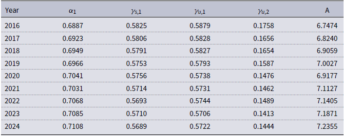
for simplicity, and calibrate the common productivity parameter to match US GDP per capita. Table A2 in Appendix A shows all parameter values.
Skill complementarity and welfare impacts of counterfactual growth in low-skilled immigrants: a two-sector economy.
Note: Parameters targeting data moments vary by year. Variables are normalized to 1 in 2016.

Figure 13 plots our results. The top panel plots the welfare change for high-skilled natives, and the bottom panel for low-skilled natives. The black dashed lines show our estimates of the increase in consumption. The black solid line shows the counterfactual path consumption would have followed had immigration not slowed down.
Introducing the second sector amplifies the gains from immigration (or the losses from the lack of it). High-skilled natives gain about 0.6% of consumption-equivalent units, and low-skilled natives 0.07% (compared to 0.5% and 0.05% in the baseline, respectively).
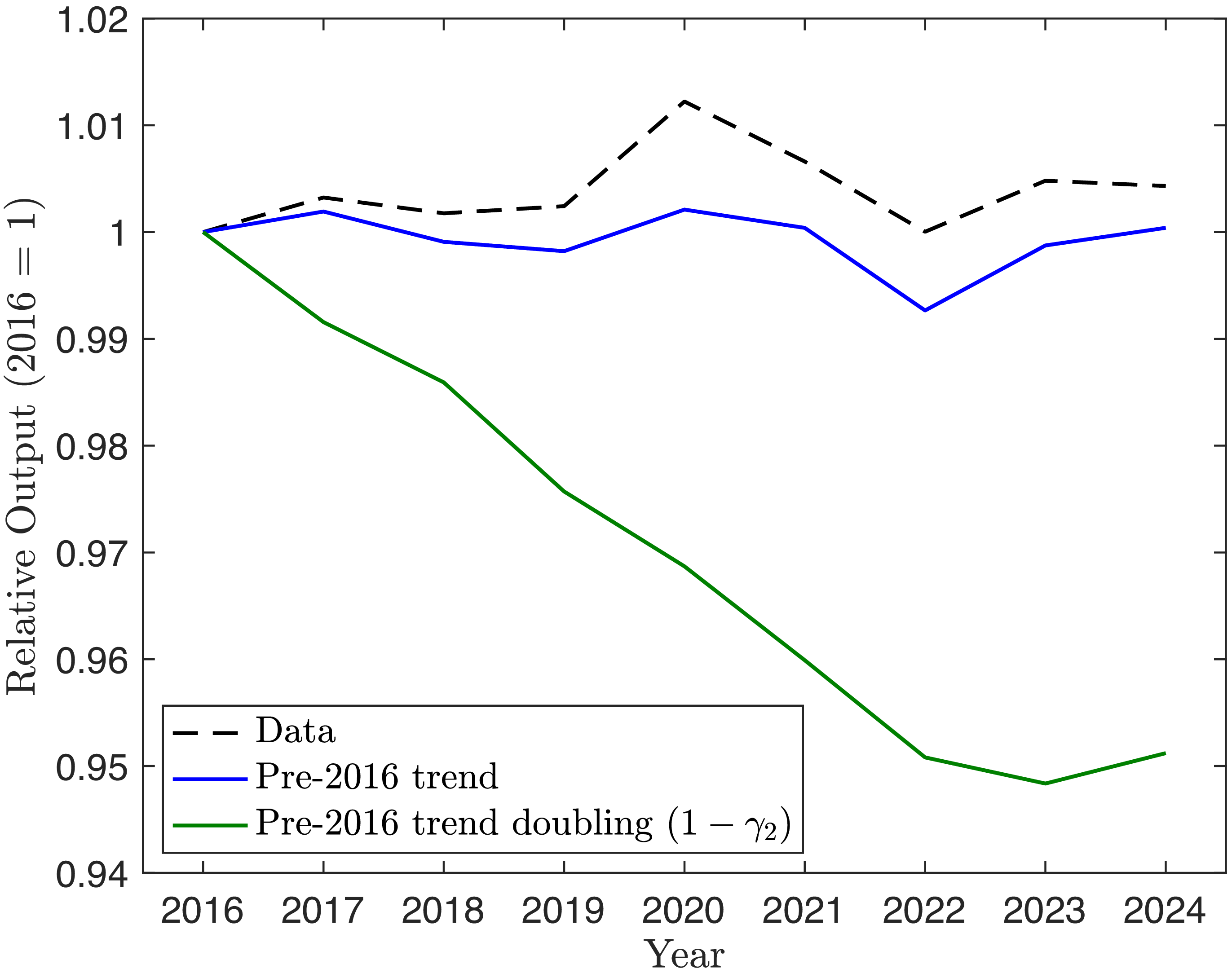
Relative output of sector 1 to sector 2.
Note: Parameters targeting data moments vary by year. Variables are normalized to 1 in 2016.

The reason why the gains are larger is that this adds a margin of adjustment to the economy: the relative amount of good 2. In fact, we show in Figure 14 that the ratio
 $Y_1/Y_2$
changes. In particular, resources flow towards the good
 $Y_2$
that is relatively more intensive in low-skilled immigrants.Footnote
7
The red lines in Figure 13 replicate these results for a larger immigrant share in sector 2. This amplifies all effects even further. Doubling the immigrant share parameter in sector 2 triples the gains for high-skilled natives (by 1.55%). Gains for the low-skilled natives increase by 1.05%. This amplification happens because, by decreasing
 $\gamma _{u,2}$
, we increase the marginal productivity of low-skilled immigrants. Thus, the same increase in employment produces a larger increase in the production possibility set.
These findings are consistent with Brinatti and Morales (Reference Brinatti and Morales2025), who finds that when immigrant intensity differs across firms, and the elasticity of substitution between natives and immigrants is larger than the demand elasticity, immigrants make the production more efficient by relocating natives to native-intensive firms. This amplifies the welfare gains from immigration.
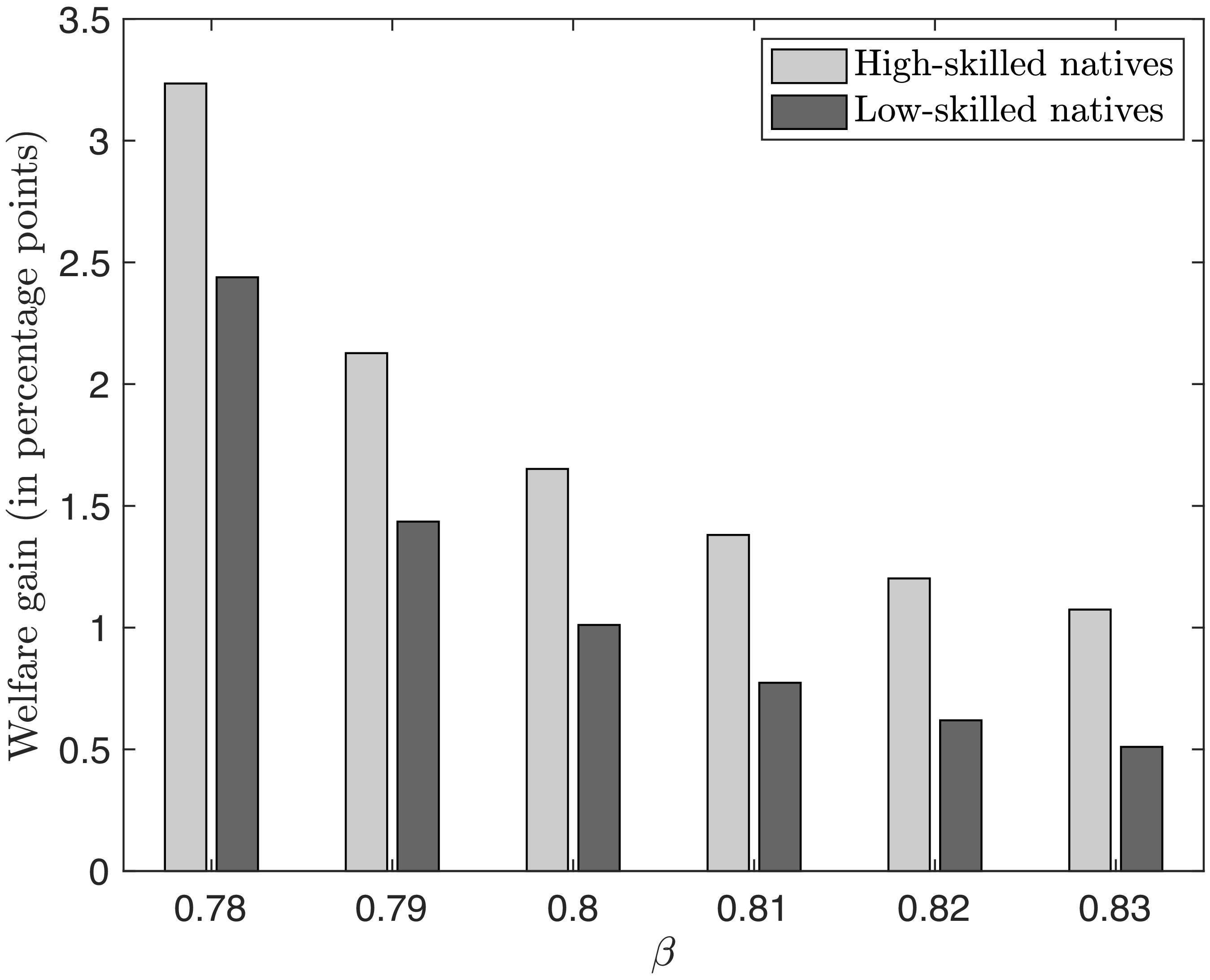
We explore changes to the size of sector 2 in Figure 15. Our benchmark sets
 $\beta = 0.8$
, so that sector 2 accounts for 20% of GDP. Making this sector larger amplifies the gains for both native types. This is because when
 $\beta$
is smaller, the marginal productivity of low-skilled immigrants is larger. Thus, as in the case with the share parameter, under a smaller value of
 $\beta$
, the expansion of the production set is larger given the same increase in low-skilled immigrants.
6.2 Construction vs. Non-construction
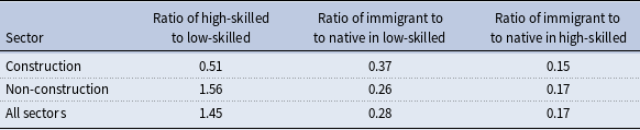
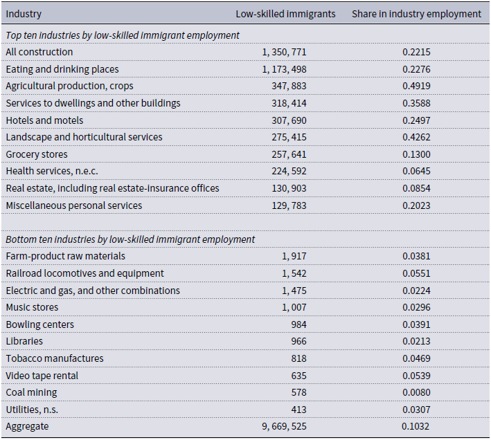
To explore quantitatively the welfare effects of low-skilled immigration in a context where one firm is intensive in their use of low-skilled workers, we map the low-skilled intensive sector with construction in the data. The choice of the construction sector is grounded in the observed pattern of immigrant employment in the U.S., as shown in Table 4. First, the construction sector on average employs twice the number of low-skilled relative to high-skilled workers, whereas on average a sector in the U.S. employs more high-skilled workers as opposed to low-skilled workers. Second, considering the ratio of low-skilled immigrants to low-skilled natives, the construction sector employs more low-skilled immigrants than the average U.S. sector, for any given number of low-skilled natives.Footnote 8 This ratio is reversed when looking at the high-skilled immigrant employment pattern in the U.S., but the ratios are close to the rest of the economy. The construction sector employs fewer high-skilled immigrants than the average U.S. sector. These patterns suggest that the construction sector becomes an important channel through which low-skilled immigration changes can affect the economy. In fact, Howard et al. (Reference Howard, Wang and Zhang2024) finds that increased immigration enforcement in the form of deportations of low-skilled immigrants reduces new housing construction and drives up the price of existing houses. Thus, to capture how the drop in low-skilled immigrants can affect welfare in the presence of heterogeneous sectors, we focus on construction and non-construction sectors.
Construction vs non-construction intensities

Table 4. Long description
A table comparing construction and non-construction sectors based on skill ratios and immigrant to native ratios. The table has three rows and four columns. The columns are labeled Sector, Ratio of high-skilled to low-skilled, Ratio of immigrant to native in low-skilled, and Ratio of immigrant to native in high-skilled. The rows are labeled Construction, Non-construction, and All sectors. Row 1: Construction, 0.51, 0.37, 0.15. Row 2: Non-construction, 1.56, 0.26, 0.17. Row 3: All sectors, 1.45, 0.28, 0.17.
Note: The ratios correspond to the average of the time period 2010–2019. The construction sector is identified using the ACS industry classification, and the non-construction sector includes all other industry classifications. All sectors represent the national average for the U.S.
Welfare gain between 2016 and 2024 with different values of
 $\beta$
.
Note: The welfare gains correspond to the scenario where
 $(1-\gamma _{u,2})$
is doubled and the model is initially calibrated for
 $\beta =0.8$
, with marginal changes in the counterfactual. The welfare gain is calculated as the difference between consumption with an increase in low-skilled immigrants and consumption without an increase.

This section maps the low-skilled sector (sector 2) with the construction sector in the data. Sector 1 maps to the rest of the economy. We calibrate the production function parameters in sector 1 to match the observed wage ratios for workers across all industries in the U.S. The corresponding parameters in sector 2 are calibrated to match the labor demands observed in the construction sector in the U.S. We set
 $\beta =0.95$
to match a share of the construction sector in the U.S. GDP of 5%. All other parameters are calibrated following the targets used in our benchmark model.
Skill complementarity and welfare impacts of counterfactual growth in low-skilled immigrants: construction vs. non-construction.
Note: Parameters targeting data moments vary by year. Variables are normalized to 1 in 2016.

Figure 16 plots the welfare for high-skilled and low-skilled natives over the years in the equilibrium and the counterfactual with more low-skilled immigrants. We compare these welfare values with the one-sector equilibrium where
 $\beta$
is equal to 1.
Welfare changes remain practically the same as in our baseline, mostly because of the small size of the new sector. In fact, expanding this sector would increase the gains for low-skilled natives of further low-skilled immigration, although these changes are likely to be small. The robustness of our results to heterogeneous sectors ratifies our confidence in our baseline results.
Both high-skilled and low-skilled natives gain from an inflow of low-skilled immigrants. Thus, even when immigrant workers are disproportionately distributed across sectors, the inflow of low-skilled immigrants generates welfare gains for natives.
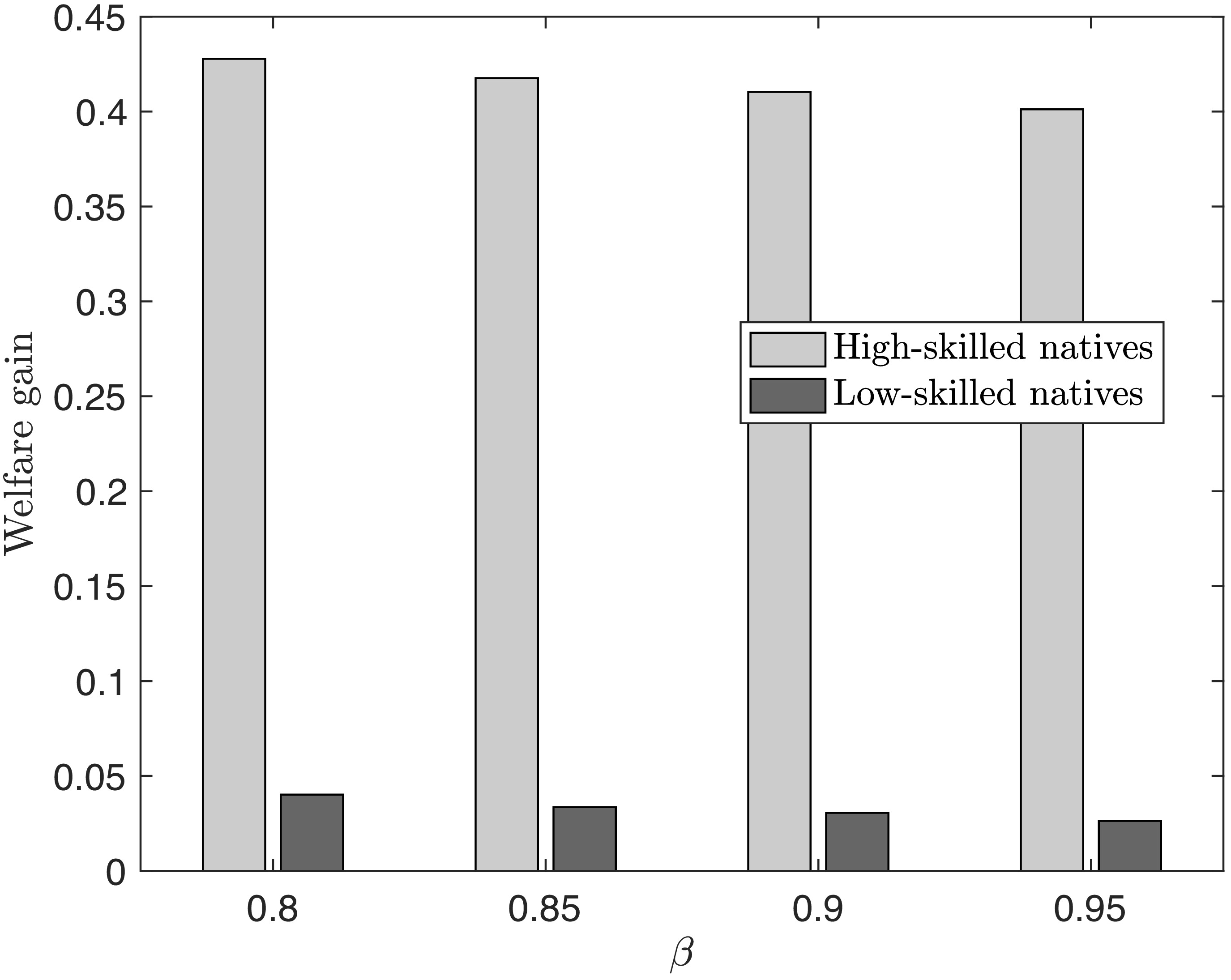
Welfare gain between 2016 and 2024 with different values of
 $\beta$
.

It is important to mention that these results hardly change as we increase the size of the low-skilled sector. Figure 17 shows that increasing this share from 5% to 20% has very little effect on the welfare changes for all natives.Footnote 9
7. Conclusion
Immigration is a subject of controversy in the United States, in particular low-skilled immigration. The main arguments center around competition and the downward pressure immigration produces on low-skilled wages.
By using a general equilibrium model of immigration, we approximate the aggregate welfare effects of recent changes in immigration. We do find that immigration reduces native wages among low-skilled workers. But we also uncover an additional effect of immigration: it provides welfare gains via general price reductions, given the increase in varieties. While low-skill nominal wages can drop with more immigration, reductions in the cost of consumption offset these effects. High-skilled workers gain via two channels: because more low-skilled workers increase their marginal productivity given complementarities; and the overall price drop effect.
Currently, aggressive anti-immigration efforts suggest welfare is bound to drop, at least for high-skilled natives. Rather than immigration, policymakers should focus on the root of the problems for low-skilled workers. Most of these are in manufacturing sectors (Clina and Rubini, Reference Clina and Rubini2024), and this sector is currently shrinking for reasons unrelated to immigration. Candidates include structural transformation, under which, as economies develop, they consume more services and less goods (see for example Herrendorf et al., Reference Herrendorf, Rogerson and Valentinyi2013; Boppart, Reference Boppart2014; Comin et al., Reference Comin, Lashkari and Mestieri2021, among others) and automation, which affects the manufacturing sector more severely than others (Acemoglu and Restrepo, Reference Acemoglu and Restrepo2022). These processes are healthy, shifting demand to higher skills, and encouraging education among the population.
Curtailing immigration will not likely affect the pace of these processes. As we show in this paper, this is more likely to hurt native workers. Rather than create an artificial demand for low-skilled workers, policymakers should focus on policies that are consistent with development, such as subsidizing education to increase the supply of high-skilled workers.
Acknowledgements
We would like to thank participants at the Midwest Macro Meeting, Kansas City Fed Brown Bag Series,and SEA Meeting for comments and feedback on the article.
Competing interests
The author(s) declare none
Appendix A. Additional tables
Calibrated parameters for all years, 2010–2024

Table A1. Long description
A table with 15 rows and 9 columns displaying calibrated parameters for the years 2010 to 2024. The columns are labeled as Year, S_j, U_n, U_j, α, γ_s, γ_u, and A. Each row corresponds to a specific year and lists the values of the parameters for that year. The table includes data moments and parameters drawn from existing research. Row 1: Year, 2010; S_j, 0.1604; U_n, 0.9082; U_j, 0.2152; α, 0.6386; γ_s, 0.5991; γ_u, 0.5963; A, 3.6882. Row 2: Year, 2011; S_j, 0.1620; U_n, 0.8859; U_j, 0.2147; α, 0.6425; γ_s, 0.5968; γ_u, 0.5962; A, 3.7173. Row 3: Year, 2012; S_j, 0.1645; U_n, 0.8575; U_j, 0.2092; α, 0.6449; γ_s, 0.5942; γ_u, 0.5965; A, 3.7630. Row 4: Year, 2013; S_j, 0.1652; U_n, 0.8427; U_j, 0.2010; α, 0.6467; γ_s, 0.5905; γ_u, 0.5960; A, 3.8019. Row 5: Year, 2014; S_j, 0.1669; U_n, 0.8248; U_j, 0.2101; α, 0.6494; γ_s, 0.5893; γ_u, 0.5959; A, 3.8390. Row 6: Year, 2015; S_j, 0.1715; U_n, 0.8111; U_j, 0.2095; α, 0.6514; γ_s, 0.5848; γ_u, 0.5923; A, 3.8960. Row 7: Year, 2016; S_j, 0.1718; U_n, 0.7868; U_j, 0.2059; α, 0.6566; γ_s, 0.5825; γ_u, 0.5879; A, 3.9367. Row 8: Year, 2017; S_j, 0.1756; U_n, 0.7678; U_j, 0.2007; α, 0.6596; γ_s, 0.5806; γ_u, 0.5828; A, 3.9838. Row 9: Year, 2018; S_j, 0.1780; U_n, 0.7580; U_j, 0.1973; α, 0.6619; γ_s, 0.5791; γ_u, 0.5827; A, 4.0350. Row 10: Year, 2019; S_j, 0.1783; U_n, 0.7486; U_j, 0.1936; α, 0.6633; γ_s, 0.5753; γ_u, 0.5793; A, 4.0932. Row 11: Year, 2020; S_j, 0.1733; U_n, 0.7044; U_j, 0.1767; α, 0.6692; γ_s, 0.5756; γ_u, 0.5738; A, 4.0478. Row 12: Year, 2021; S_j, 0.1773; U_n, 0.7091; U_j, 0.1880; α, 0.6686; γ_s, 0.5714; γ_u, 0.5731; A, 4.1631. Row 13: Year, 2022; S_j, 0.1803; U_n, 0.7006; U_j, 0.1862; α, 0.6722; γ_s, 0.5693; γ_u, 0.5744; A, 4.1866. Row 14: Year, 2023; S_j, 0.1856; U_n, 0.6898; U_j, 0.1901; α, 0.6734; γ_s, 0.5710; γ_u, 0.5706; A, 4.2138. Row 15: Year, 2024; S_j, 0.1928; U_n, 0.6769; U_j, 0.1936; α, 0.6754; γ_s, 0.5689; γ_u, 0.5722; A, 4.2452.
Note: The labor supply for high-skilled natives (
 $S_{n}$
) is normalized to 1 for all years, and the other labor types (
 $S_{i}$
,
 $U_{n}$
,
 $U_{i}$
) are calibrated as a share of the high-skilled natives for each year.
Calibrated parameters with two sectors

Table A2. Long description
A table showing calibrated parameters with two sectors over several years. The table has 9 rows and 6 columns. The columns are labeled Year, alpha 1, gamma 1, gamma 1, gamma 2, and A. The rows are labeled with years from 2016 to 2024. Row 1: Year, 2016; alpha 1, 0.6887; gamma 1, 0.5825; gamma 1, 0.5879; gamma 2, 0.1758; A, 6.7474. Row 2: Year, 2017; alpha 1, 0.6923; gamma 1, 0.5806; gamma 1, 0.5828; gamma 2, 0.1656; A, 6.8240. Row 3: Year, 2018; alpha 1, 0.6949; gamma 1, 0.5791; gamma 1, 0.5827; gamma 2, 0.1654; A, 6.9059. Row 4: Year, 2019; alpha 1, 0.6966; gamma 1, 0.5753; gamma 1, 0.5793; gamma 2, 0.1587; A, 7.0027. Row 5: Year, 2020; alpha 1, 0.7041; gamma 1, 0.5756; gamma 1, 0.5738; gamma 2, 0.1476; A, 6.9177. Row 6: Year, 2021; alpha 1, 0.7031; gamma 1, 0.5714; gamma 1, 0.5731; gamma 2, 0.1462; A, 7.1127. Row 7: Year, 2022; alpha 1, 0.7068; gamma 1, 0.5693; gamma 1, 0.5744; gamma 2, 0.1489; A, 7.1405. Row 8: Year, 2023; alpha 1, 0.7085; gamma 1, 0.5710; gamma 1, 0.5706; gamma 2, 0.1413; A, 7.1871. Row 9: Year, 2024; alpha 1, 0.7108; gamma 1, 0.5689; gamma 1, 0.5722; gamma 2, 0.1444; A, 7.2355.
Note: The table reports only the time-varying parameters that are separately calibrated in the two-sector model. The labor supply values correspond to Table A1.
 $\gamma _{u,2}$
is calibrated such that,
 $(1-\gamma _{u,2})=2\times (1-\gamma _{u,1})$
.
 $\alpha _{2}$
and
 $\gamma _{s,2}$
are 0 by construction. Parameters that do not vary across years are
 $\sigma$
,
 $\eta$
,
 $\rho _{s}$
,
 $\rho _{u}$
,
 $f_{e}$
, and
 $\theta$
, use the values in Table 1.
 $\beta$
is assumed 0.8 in this calibration, and Figure 15 reports the welfare estimates with alternate values of
 $\beta$
.
Low-skilled immigrant employment across ACS industries

Table A3. Long description
A table comparing low-skilled immigrant employment across various industries. The table has 20 rows and 3 columns. The columns are labeled ‘Industry’, ‘Low-skilled immigrants’, and ‘Share in industry employment’. The table is divided into two sections: top ten industries and bottom ten industries by low-skilled immigrant employment. Each row lists an industry, the number of low-skilled immigrants employed, and the share of industry employment. Notable trends include the construction industry having the highest number of low-skilled immigrants employed, while industries like farm-product raw materials and railroad locomotives have lower employment shares.
Source: American Community Survey (2010–2019).
Appendix B. Counterfactual effects on immigrants
Skill complementarity and welfare impacts of counterfactual growth in low-skilled immigrants: immigrant workers.
Note: Parameters targeting data moments vary by year. Variables are normalized to 1 in 2016.

Appendix C. Sensitivity to
 $\boldsymbol{\sigma}$

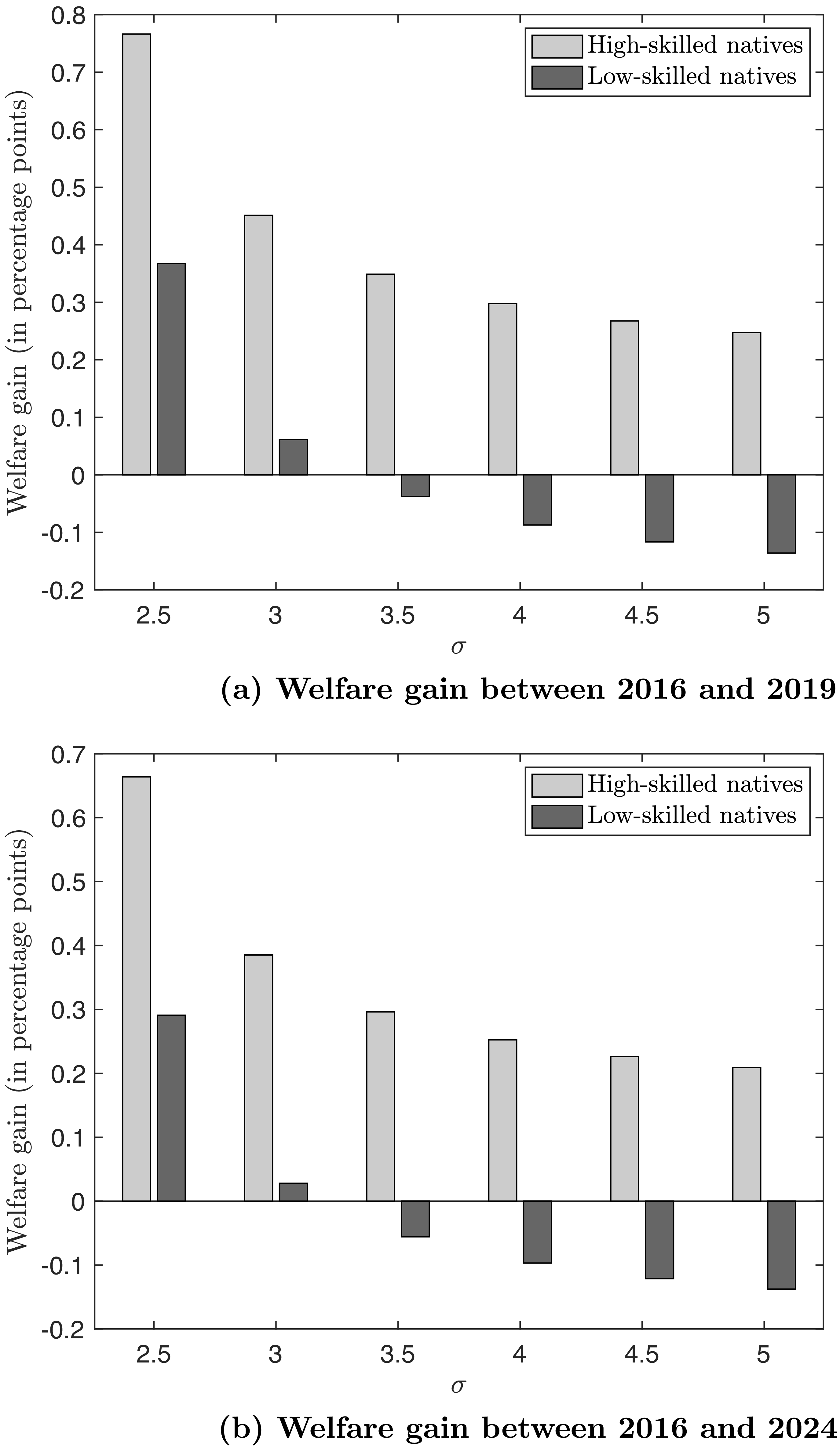
The market-size channel plays an important role and is key to non-negative welfare gains from immigration. As such, we perform a sensitivity analysis on
 $\sigma$
, the parameter governing this channel. We quantify the welfare gains from the counterfactual increase in low-skilled immigrants under alternative values of
 $\sigma$
. Figure C1 shows these welfare gains. The welfare gains from additional low-skilled immigrants are decreasing in
 $\sigma$
. The high-skilled natives still enjoy positive welfare gains. However, when the love for variety channel is weak, the low-skilled natives have negative welfare gains. This negative gains arise because the variety channel in equation (17) fails to compensate for the downward pressure on low-skilled native welfare coming from the standard wage channel under high values of
 $\sigma$
. Thus, this parameter becomes key to determining the welfare effects of immigration.
Sensitivity of welfare gains to
 $\sigma$
.








 β
 (1−γu,2)
 β=0.8

 β

 σ

 Open access

