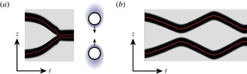
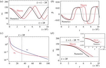
1 Introduction
In biological systems, cells and microorganisms are moving spontaneously and autonomously by consuming energy from adenosine triphosphate (ATP) hydrolysis. The size and swimming speed of bacteria are small, and their self-propulsion is described by low Reynolds number hydrodynamics. In an attempt to capture the generic mechanism of the self-propulsion, various mathematical models have been investigated. One of these is the squirmer model, which considers the flow field created by the beating of cilia on the body of a microorganism and/or the deformation of its body surface (Lighthill Reference Lighthill1952; Blake Reference Blake1971). The problem then becomes a matter of solving the Stokes equation under the boundary conditions of finite velocity on the surface of the body in the normal and/or tangential directions. The translational and angular velocities of a single squirmer are well understood (Stone & Samuel Reference Stone and Samuel1996). Apart from that model, there have been several attempts to find other classes of self-propulsion. The simplest extension of the model is to include an additional scalar field such as the concentration, electric or temperature field. A Janus particle, which is an asymmetric particle with two different surface properties, creates a gradient of the field around the particle, and thus, in turn, causes it to move spontaneously (Paxton et al. Reference Paxton, Kistler, Olmeda, Sen, St.Angelo, Cao, Mallouk, Lammert and Crespi2004; Howse et al. Reference Howse, Jones, Ryan, Gough, Vafabakhsh and Golestanian2007; Jiang, Yoshinaga & Sano Reference Jiang, Yoshinaga and Sano2010). This motion is similar to phoresis, except that the gradient is self-generated instead of imposed. This mechanism is thus called self-phoresis.
The squirmer and Janus particles have intrinsic asymmetry, and therefore the swimming direction is set by the polar direction of the asymmetry of each particle. This simplifies the problem: there is a linear relation between the self-propulsion speed and the magnitude of the asymmetry. This idea may also be extended toward self-propulsion of a geometrically asymmetric object with a uniform surface property (Tsemakh, Lavrenteva & Nir Reference Tsemakh, Lavrenteva and Nir2004; Shklyaev, Brady & Crdova-Figueroa Reference Shklyaev, Brady and Crdova-Figueroa2014). On the other hand, cells often break symmetry to choose the direction of motion (Yam et al. Reference Yam, Wilson, Ji, Hebert, Barnhart, Dye, Wiseman, Danuser and Theriot2007). This phenomenon is not captured by the squirmer and Janus particles, and therefore another class of self-propulsion must be considered. As a step in this direction, various mathematical models that include the internal polarity field have been proposed (Shao, Rappel & Levine Reference Shao, Rappel and Levine2010; Tjhung, Marenduzzo & Cates Reference Tjhung, Marenduzzo and Cates2012; Ziebert, Swaminathan & Aranson Reference Ziebert, Swaminathan and Aranson2012). In these models, it has been observed that spontaneous symmetry-breaking results in directional motion.
Along this line, it was recently found that non-living chemically driven systems exhibit self-propulsion (Toyota et al. Reference Toyota, Maru, Hanczyc, Ikegami and Sugawara2009; Thutupalli, Seemann & Herminghaus Reference Thutupalli, Seemann and Herminghaus2011; Izri et al. Reference Izri, van der Linden, Michelin and Dauchot2014). In these systems, a drop may produce or consume chemical molecules in such a way that the system is away from an equilibrium state. The flux couples with the motion and results in an asymmetric concentration distribution. Once the symmetry is broken, the surface tension becomes anisotropic and this creates flow both inside and outside the drop. This motion, which occurs along the given gradient of concentration and/or temperature fields, is known as the Marangoni effect (Fedosov Reference Fedosov1956; Young, Goldstein & Block Reference Young, Goldstein and Block1959). The self-propulsive motion using the Marangoni effect resulting from a chemical reaction was first proposed as a reactive drop (Ryazantsev Reference Ryazantsev1985), and later its mechanism was theoretically reformulated as a bifurcation phenomena (Yabunaka, Ohta & Yoshinaga Reference Yabunaka, Ohta and Yoshinaga2012; Yoshinaga et al. Reference Yoshinaga, Nagai, Sumino and Kitahata2012; Yoshinaga Reference Yoshinaga2014). In these studies, the reduced nonlinear equations were derived from the coupled advection–diffusion and hydrodynamic equations. A similar idea was considered for the auto-phoretic motion, which is the self-phoretic motion of a Janus particle due to a nonlinear coupling of an isotropic chemical reaction and advection (Michelin, Lauga & Bartolo Reference Michelin, Lauga and Bartolo2013).
Although the self-propulsion of an isolated particle/drop is well understood, there is still only a limited understanding of the interactions between them. There have been intensive numerical studies of interactions between squirmers (Ishikawa, Simmonds & Pedley Reference Ishikawa, Simmonds and Pedley2006) and between a squirmer and a wall (Spagnolie & Lauga Reference Spagnolie and Lauga2012). In particular, understanding of the squirmer/wall system has recently increased, and numerical simulations have revealed the bound state near the wall (Li & Ardekani Reference Li and Ardekani2014). These results are consistent with those from an analysis of the equation of motion of a squirmer, using a technique for analysing dynamical systems (Ishimoto & Gaffney Reference Ishimoto and Gaffney2013). Even for Janus particles, numerical simulations near a wall have only been performed very recently (Uspal et al. Reference Uspal, Popescu, Dietrich and Tasinkevych2015).
In this work, we discuss the interaction between self-propelled drops. In particular, we focus on head-on collisions between two drops. As we will discuss, the interaction arises from hydrodynamics and a concentration overlap. The hydrodynamic interaction has been discussed in terms of the squirmer model, in which only the velocity field is treated. The concentration overlap has been discussed in the context of reaction–diffusion systems; in that case, the concentration fields are analysed without considering the hydrodynamics, and thus mechanics does not play a role (Ohta, Kiyose & Mimura Reference Ohta, Kiyose and Mimura1997; Ohta Reference Ohta2001; Bode et al. Reference Bode, Liehr, Schenk and Purwins2002; Nishiura, Teramoto & Ueda Reference Nishiura, Teramoto and Ueda2003; Ei, Mimura & Nagayama Reference Ei, Mimura and Nagayama2006). The primary questions are which effect dominates the interaction and when do cross-overs occur. To answer these questions, we consider the theory for two interacting drops that are separated far away from each other. This is an extension of the theory for a single drop discussed in Yabunaka et al. (Reference Yabunaka, Ohta and Yoshinaga2012), Yoshinaga (Reference Yoshinaga2014). Other studies (Golovin, Nir & Pismen Reference Golovin, Nir and Pismen1995; Lavrenteva, Leshansky & Nir Reference Lavrenteva, Leshansky and Nir1999) have used a boundary-value approach to investigate the interaction that arises from hydrodynamics and the concentration (or heat) field. Our model shares a similar philosophy, although we focus on the equations of motion of a reduced description and drops with unsteady motion, rather than stationary speed. The main difference is that we use a diffuse-interface approach, and because of this, both analytical and numerical solutions become tractable. We will discuss the similarities and differences in § 8.
We also develop numerical simulations of isolated as well as interacting drops. This enables us to investigate the effect of advection of the chemical component; a complete analytical investigation of this has not been previously performed (Yabunaka et al. Reference Yabunaka, Ohta and Yoshinaga2012; Yoshinaga Reference Yoshinaga2014). We confirm that the convection of the chemical component does not change the essential bifurcation of a single drop, but it suppresses the drift instability; this supports previously presented theories (Yabunaka et al. Reference Yabunaka, Ohta and Yoshinaga2012; Yoshinaga Reference Yoshinaga2014). For interacting drops, we will numerically investigate the dynamics of collisions; this complements our theoretical calculations.
The interaction between two self-propelled particles is distinct from that seen in conventional passive systems, where particles and drops are driven by external forces (Jeffrey & Onishi Reference Jeffrey and Onishi1984). The dominant hydrodynamic interaction in the far field does not arise from a Stokeslet but from a source doublet or a stresslet depending on the mode (
 $l=1$
or
 $l=2$
) for the expansion of the slip velocity, as expressed by spherical harmonics (Lauga & Powers Reference Lauga and Powers2009; Pak & Lauga Reference Pak and Lauga2014). In addition, our system is different from either the squirmer or the Janus particle; it does not have a specific intrinsic polarity, but polarity spontaneously appears when the bifurcation parameter exceeds a threshold value. Consequently, the direction of motion of a drop may change without rotation.
In the remaining sections, we formulate a model for chemically driven self-propulsion that uses the Marangoni effect. To prepare for the main parts, in § 2, we compute the flow field and resulting velocity of a drop under a given distribution of the surface tension. In § 3, we summarize the spontaneous motion of an isolated drop. In § 4, we derive the hydrodynamic and concentration-mediated interactions between two drops, and the equations of motion for two interacting drops are formulated in § 5. Numerical results for isolated and colliding drops are presented in §§ 6 and 7, respectively. We compare the numerical results with our theoretical analysis of § 4. We conclude with § 8, which summarizes our results.
2 An isolated drop under a given concentration gradient
Before discussing the interaction between spherical drops, we first calculate the flow field around a spherical drop driven by an arbitrary distribution of the surface tension. The axisymmetric flow field around the drop has been studied (Young et al. Reference Young, Goldstein and Block1959; Levan Reference Levan1981; Kitahata et al. Reference Kitahata, Yoshinaga, Nagai and Sumino2011). Here we do not assume that the system is axisymmetric; thus, instead of expanding the surface tension in terms of Legendre polynomials, we use spherical harmonics:
 $$\begin{eqnarray}\unicode[STIX]{x1D6FE}(\unicode[STIX]{x1D703},\unicode[STIX]{x1D711})=\mathop{\sum }_{l,m}\unicode[STIX]{x1D6FE}_{lm}Y_{l}^{m}(\unicode[STIX]{x1D703},\unicode[STIX]{x1D711}).\end{eqnarray}$$
The velocity fields inside and outside the drop are expanded as follows:
 $$\begin{eqnarray}\displaystyle & \displaystyle \boldsymbol{v}^{(i)}=\mathop{\sum }_{l,m}\boldsymbol{v}_{lm}^{(i)}=\mathop{\sum }_{l,m}[f_{lm}^{(i)}(r)\boldsymbol{Y}_{lm}(\unicode[STIX]{x1D703},\unicode[STIX]{x1D711})+g_{lm}^{(i)}(r)\boldsymbol{\unicode[STIX]{x1D6F9}}_{lm}(\unicode[STIX]{x1D703},\unicode[STIX]{x1D711})] & \displaystyle\end{eqnarray}$$
 $$\begin{eqnarray}\displaystyle & \displaystyle \boldsymbol{v}^{(o)}=\mathop{\sum }_{l,m}\boldsymbol{v}_{lm}^{(o)}=\mathop{\sum }_{l,m}[f_{lm}^{(o)}(r)\boldsymbol{Y}_{lm}(\unicode[STIX]{x1D703},\unicode[STIX]{x1D711})+g_{lm}^{(o)}(r)\boldsymbol{\unicode[STIX]{x1D6F9}}_{lm}(\unicode[STIX]{x1D703},\unicode[STIX]{x1D711})], & \displaystyle\end{eqnarray}$$
where the outer and inner fields are indicated by the superscripts
 $(o)$
and
 $(i)$
, respectively, and the vector spherical harmonics are defined by using the scalar spherical harmonics
 $Y_{l}^{m}(\unicode[STIX]{x1D703},\unicode[STIX]{x1D711})$
, as follows:
 $$\begin{eqnarray}\displaystyle & \displaystyle \boldsymbol{Y}_{lm}=Y_{l}^{m}\hat{\boldsymbol{r}} & \displaystyle\end{eqnarray}$$
 $$\begin{eqnarray}\displaystyle & \displaystyle \unicode[STIX]{x1D733}_{lm}=r\unicode[STIX]{x1D735}Y_{l}^{m}, & \displaystyle\end{eqnarray}$$
where
 $\hat{\boldsymbol{r}}$
is a unit normal vector. Since the flow field is driven by the gradient of the surface tension, one of the vector spherical harmonics,
 $\unicode[STIX]{x1D731}_{lm}=\boldsymbol{r}\times \unicode[STIX]{x1D735}Y_{l}^{m}$
, which is in the tangential direction perpendicular to
 $\unicode[STIX]{x1D733}_{lm}$
, does not appear in this expansion. Note that
 $f_{lm}(r)$
and
 $g_{lm}(r)$
are determined from the boundary conditions, as discussed below.
We consider a spherical drop that is moving with velocity
 $\boldsymbol{u}$
in an arbitrary direction. At any point
 $(\unicode[STIX]{x1D703},\unicode[STIX]{x1D711})$
on the drop surface, the velocity is expressed as
 $$\begin{eqnarray}\boldsymbol{u}=\mathop{\sum }_{m}u_{m}(\boldsymbol{Y}_{1,m}(\unicode[STIX]{x1D703},\unicode[STIX]{x1D711})+\unicode[STIX]{x1D733}_{1,m}(\unicode[STIX]{x1D703},\unicode[STIX]{x1D711})),\end{eqnarray}$$
which can be expressed in the Cartesian coordinates as (see (2.11))
 $$\begin{eqnarray}\boldsymbol{u}=\left(\sqrt{\frac{3}{4\unicode[STIX]{x03C0}}}\frac{u_{-1}-u_{1}}{\sqrt{2}},i\sqrt{\frac{3}{4\unicode[STIX]{x03C0}}}\frac{-u_{-1}-u_{1}}{\sqrt{2}},\sqrt{\frac{3}{4\unicode[STIX]{x03C0}}}u_{0}\right).\end{eqnarray}$$
We will assume the velocity of the drop is sufficiently slow that the Reynolds number is near zero, and thus it satisfies the Stokes equation except over the surface of the drop
 $r=R$
 $$\begin{eqnarray}\displaystyle & \displaystyle \unicode[STIX]{x1D702}^{(i)}\unicode[STIX]{x1D6FB}^{2}\boldsymbol{v}^{(i)}-\unicode[STIX]{x1D735}p^{(i)}=0, & \displaystyle\end{eqnarray}$$
 $$\begin{eqnarray}\displaystyle & \displaystyle \unicode[STIX]{x1D702}^{(o)}\unicode[STIX]{x1D6FB}^{2}\boldsymbol{v}^{(o)}-\unicode[STIX]{x1D735}p^{(o)}=0. & \displaystyle\end{eqnarray}$$
The pressure
 $p$
is determined from the incompressibility condition
 $$\begin{eqnarray}\unicode[STIX]{x1D735}\boldsymbol{\cdot }\boldsymbol{v}=0.\end{eqnarray}$$
The boundary conditions on
 $r=R$
are
 $$\begin{eqnarray}\displaystyle & \displaystyle \boldsymbol{v}^{(o)}\boldsymbol{\cdot }\hat{\boldsymbol{r}}=\boldsymbol{v}^{(i)}\boldsymbol{\cdot }\hat{\boldsymbol{r}}=\boldsymbol{u}\boldsymbol{\cdot }\hat{\boldsymbol{r}} & \displaystyle\end{eqnarray}$$
 $$\begin{eqnarray}\displaystyle & \displaystyle \boldsymbol{v}^{(o)}\boldsymbol{\cdot }\hat{\boldsymbol{t}}=\boldsymbol{v}^{(i)}\boldsymbol{\cdot }\hat{\boldsymbol{t}} & \displaystyle\end{eqnarray}$$
 $$\begin{eqnarray}\displaystyle & \displaystyle \unicode[STIX]{x1D70E}_{nt}^{(i)}(R)\hat{\boldsymbol{t}}=\unicode[STIX]{x1D70E}_{nt}^{(o)}(R)\hat{\boldsymbol{t}}+\frac{1}{R}\unicode[STIX]{x1D735}_{s}\unicode[STIX]{x1D6FE}, & \displaystyle\end{eqnarray}$$
where
 $\hat{\boldsymbol{t}}$
is the unit tangent vectors. The conditions (2.11) and (2.12) are continuity of the velocity field across the interface, and (2.13) implies that the forces are balanced at the interface, that is, the jump of shear stress across the interface due to the force created by the inhomogeneous surface tension (Scriven Reference Scriven1960). The system is force free; there is no mechanical force acting on the drop,
 $$\begin{eqnarray}\boldsymbol{F}=\int \text{d}S\,\unicode[STIX]{x1D70E}^{(o)}(R)\boldsymbol{\cdot }\boldsymbol{n}=0,\end{eqnarray}$$
where the integral is taken over the surface of the drop. The stress balance in the normal direction is automatically satisfied for the
 $l=1$
mode and determines the shape of the drop for
 $l\geqslant 2$
.
The solution of the Stokes equations for this system, (2.8) and (2.9), can be decomposed into two parts: one for
 $l=1$
and the other for
 $l\geqslant 2$
. For
 $l=1$
,
 $$\begin{eqnarray}\displaystyle & \displaystyle \boldsymbol{v}_{1,m}^{(i)}=u_{m}\left(\left[-\frac{3}{2}\left(\frac{r}{R}\right)^{2}+\frac{5}{2}\right]\boldsymbol{Y}_{1,m}+\left[-3\left(\frac{r}{R}\right)^{2}+\frac{5}{2}\right]\unicode[STIX]{x1D733}_{1,m}\right) & \displaystyle\end{eqnarray}$$
 $$\begin{eqnarray}\displaystyle & \displaystyle \boldsymbol{v}_{1,m}^{(o)}=u_{m}\left[\left(\frac{R}{r}\right)^{3}\boldsymbol{Y}_{1,m}-\frac{1}{2}\left(\frac{R}{r}\right)^{3}\unicode[STIX]{x1D733}_{1,m}\right] & \displaystyle\end{eqnarray}$$
 $$\begin{eqnarray}\displaystyle & \displaystyle p^{(o)}=0 & \displaystyle\end{eqnarray}$$
 $$\begin{eqnarray}\displaystyle & \displaystyle p^{(i)}=-\mathop{\sum }_{m}\frac{10\unicode[STIX]{x1D702}^{(i)}\unicode[STIX]{x1D6FE}_{1,m}}{R(3\unicode[STIX]{x1D702}^{(i)}+2\unicode[STIX]{x1D702}^{(o)})}\frac{r}{R}Y_{1}^{m}(\unicode[STIX]{x1D703},\unicode[STIX]{x1D711})=-\mathop{\sum }_{m}\frac{15\unicode[STIX]{x1D702}^{(i)}u_{m}}{R}\frac{r}{R}Y_{1}^{m}(\unicode[STIX]{x1D703},\unicode[STIX]{x1D711}) & \displaystyle\end{eqnarray}$$
and for
 $l\geqslant 2$
 $$\begin{eqnarray}\displaystyle \boldsymbol{v}_{l,m}^{(i)} & = & \displaystyle \frac{\unicode[STIX]{x1D6FE}_{lm}}{2(\unicode[STIX]{x1D702}^{(i)}+\unicode[STIX]{x1D702}^{(o)})(2l+1)}\left(l(l+1)\left[\left(\frac{r}{R}\right)^{l+1}-\left(\frac{r}{R}\right)^{l-1}\right]\boldsymbol{Y}_{lm}\right.\nonumber\\ \displaystyle & & \displaystyle \left.+\left[-(l+1)\left(\frac{r}{R}\right)^{l-1}+(l+3)\left(\frac{r}{R}\right)^{l+1}\right]\unicode[STIX]{x1D733}_{lm}\right)\end{eqnarray}$$
 $$\begin{eqnarray}\displaystyle \boldsymbol{v}_{l,m}^{(o)} & = & \displaystyle \frac{\unicode[STIX]{x1D6FE}_{lm}}{2(\unicode[STIX]{x1D702}^{(i)}+\unicode[STIX]{x1D702}^{(o)})(2l+1)}\left(l(l+1)\left[\left(\frac{R}{r}\right)^{l}-\left(\frac{R}{r}\right)^{l+2}\right]\boldsymbol{Y}_{lm}\right.\nonumber\\ \displaystyle & & \displaystyle \left.+\left[-(l-2)\left(\frac{R}{r}\right)^{l}+l\left(\frac{R}{r}\right)^{l+2}\right]\unicode[STIX]{x1D733}_{lm}\right)\end{eqnarray}$$
 $$\begin{eqnarray}\displaystyle & \displaystyle p^{(o)}=\mathop{\sum }_{l,m}\frac{\unicode[STIX]{x1D702}^{(o)}\unicode[STIX]{x1D6FE}_{lm}}{R(\unicode[STIX]{x1D702}^{(i)}+\unicode[STIX]{x1D702}^{(o)})}\frac{l(2l-1)}{2l+1}\left(\frac{R}{r}\right)^{l+1}Y_{l}^{m}(\unicode[STIX]{x1D703},\unicode[STIX]{x1D711}) & \displaystyle\end{eqnarray}$$
 $$\begin{eqnarray}\displaystyle & \displaystyle p^{(i)}=\mathop{\sum }_{l,m}\frac{\unicode[STIX]{x1D702}^{(i)}\unicode[STIX]{x1D6FE}_{lm}}{R(\unicode[STIX]{x1D702}^{(i)}+\unicode[STIX]{x1D702}^{(o)})}\frac{(l+1)(2l+3)}{2l+1}\left(\frac{r}{R}\right)^{l}Y_{l}^{m}(\unicode[STIX]{x1D703},\unicode[STIX]{x1D711}). & \displaystyle\end{eqnarray}$$
Because of the force-free condition, the velocity field for
 $l=1$
decays as
 $1/r^{3}$
and not as
 $1/r$
. This occurs because the motion is not driven by the Stokeslet but by the quadrupole (source dipole). The velocity of the drop is
 $$\begin{eqnarray}u_{m}=-\frac{2\unicode[STIX]{x1D6FE}_{1,m}}{3(3\unicode[STIX]{x1D702}^{(i)}+2\unicode[STIX]{x1D702}^{(o)})}.\end{eqnarray}$$
The axisymmetric case corresponds to
 $\unicode[STIX]{x1D6FE}_{l,m}=0$
for
 $m\neq 0$
. This result is consistent with that of Young et al.
Reference Young, Goldstein and Block1959 (except for typographical errors; see Levan Reference Levan1981, Kitahata et al.
Reference Kitahata, Yoshinaga, Nagai and Sumino2011). Note that the coefficient may depend on the definition of the normalization factor in the spherical harmonics.
3 Self-propelled motion of a single drop
In this section, we summarize the self-propelled motion of an isolated drop. The details for the analysis of this model can be found in Yabunaka et al. (Reference Yabunaka, Ohta and Yoshinaga2012). We consider the dynamics of the concentration field,
 $c(\boldsymbol{r})$
, of a third dilute component
 $$\begin{eqnarray}\frac{\unicode[STIX]{x2202}c}{\unicode[STIX]{x2202}t}+\boldsymbol{v}\boldsymbol{\cdot }\unicode[STIX]{x1D735}c=D\unicode[STIX]{x1D6FB}^{2}c-\unicode[STIX]{x1D705}(c-c_{\infty })+A\unicode[STIX]{x1D6E9}(R-|\boldsymbol{r}-\boldsymbol{r}_{G}|).\end{eqnarray}$$
The system is driven away from equilibrium, where the drop is stationary, by the source term described by the step function
 $\unicode[STIX]{x1D6E9}(x)$
with the coefficient
 $A$
. When
 $A>0$
, the drop produces chemical molecules, while when
 $A<0$
, the drop consumes them. Note that we do not use the comoving frame with the drop; therefore, the advection term in (3.1) describes only the advection due to the flow. In a comoving frame, there will be an additional contribution due to the fact that the drop is moving. In our model, this effect is included in the last term in (3.1).
Based on the diffuse-interface model (Hohenberg & Halperin Reference Hohenberg and Halperin1977; Anderson, McFadden & Wheeler Reference Anderson, Mcfadden and Wheeler1998), we describe the drop as a binary mixture, where
 $\unicode[STIX]{x1D719}=1$
inside the drop and
 $\unicode[STIX]{x1D719}=-1$
outside. The dynamics is given by the Cahn–Hilliard equation with advection:
 $$\begin{eqnarray}\frac{\unicode[STIX]{x2202}\unicode[STIX]{x1D719}}{\unicode[STIX]{x2202}t}+\boldsymbol{v}\boldsymbol{\cdot }\unicode[STIX]{x1D735}\unicode[STIX]{x1D719}=\unicode[STIX]{x1D735}\boldsymbol{\cdot }L\unicode[STIX]{x1D735}\frac{\unicode[STIX]{x1D6FF}F}{\unicode[STIX]{x1D6FF}\unicode[STIX]{x1D719}},\end{eqnarray}$$
where the mobility
 $L$
is assumed to be constant. The free energy has a double-well type potential:
 $$\begin{eqnarray}F=\int _{\unicode[STIX]{x1D6FA}}\left[-\frac{1}{2}\unicode[STIX]{x1D719}^{2}+\frac{1}{4}\unicode[STIX]{x1D719}^{4}+\frac{B(c)}{2}|\unicode[STIX]{x1D735}\unicode[STIX]{x1D719}|^{2}\right],\end{eqnarray}$$
where
 $\unicode[STIX]{x1D6FA}$
is the entire domain of the system. The interfacial energy is dependent on the concentration field
 $c(\boldsymbol{r})$
. We assume the linear relation
 $$\begin{eqnarray}B(c)=B_{0}+B_{1}c(\boldsymbol{r}),\end{eqnarray}$$
which is characterized by two parameters,
 $B_{0}$
and
 $B_{1}$
. The benefit of this approach is that we do not need to solve the Stokes equation with moving boundary conditions. The force acting on the fluid is given by
 $$\begin{eqnarray}\boldsymbol{f}=-\unicode[STIX]{x1D719}\unicode[STIX]{x1D735}\frac{\unicode[STIX]{x1D6FF}F}{\unicode[STIX]{x1D6FF}\unicode[STIX]{x1D719}}-c\unicode[STIX]{x1D735}\frac{\unicode[STIX]{x1D6FF}F}{\unicode[STIX]{x1D6FF}c};\end{eqnarray}$$
this is generated by the surface tension and thus localises at the interface between the drop and the surrounding fluid. The force can be expressed in divergence form as
 $$\begin{eqnarray}\boldsymbol{f}=\unicode[STIX]{x1D735}\boldsymbol{\cdot }\unicode[STIX]{x1D6F1},\end{eqnarray}$$
where the stress is
 $$\begin{eqnarray}\unicode[STIX]{x1D6F1}_{ij}=B(c)\unicode[STIX]{x1D735}_{i}\unicode[STIX]{x1D719}\unicode[STIX]{x1D735}_{j}\unicode[STIX]{x1D719}+\text{isotropic terms}.\end{eqnarray}$$
The isotropic terms merely modify the reference pressure and thus we will not discuss them further. In the thin-interface limit, the concentration in the region of the diffused interface (in bulk) can be represented by the surface concentration. Then, (3.4), expressing the gradient energy at a given bulk concentration, generally leads to a nonlinear dependence of the surface tension on the surface concentration. However, the surface tension can be linearly expanded with respect to the deviation from a constant value
 $c_{0}$
of the surface concentration, provided that the deviation across the entire surface is small:
 $$\begin{eqnarray}\unicode[STIX]{x1D6FE}(c_{I})=\unicode[STIX]{x1D6FE}(c_{0})+\left.\frac{\unicode[STIX]{x2202}\unicode[STIX]{x1D6FE}(c_{0})}{\unicode[STIX]{x2202}c_{I}}(c_{I}-c_{0})\right|_{\boldsymbol{r}=\boldsymbol{R}},\end{eqnarray}$$
where
 $c_{I}$
represents the surface concentration. We may also be able to consider a more realistic dependence by replacing the functional form in (3.4) with a logarithmic function.
Instead of (2.8) and (2.9), we solve the following single Stokes equation with the force
 $\boldsymbol{f}$
for the entire space under the incompressibility condition
 $\unicode[STIX]{x1D735}\boldsymbol{\cdot }\boldsymbol{v}=0$
:
 $$\begin{eqnarray}\unicode[STIX]{x1D702}\unicode[STIX]{x1D6FB}^{2}\boldsymbol{v}-\unicode[STIX]{x1D735}p+\boldsymbol{f}=0.\end{eqnarray}$$
We also assume
 $\unicode[STIX]{x1D702}^{(o)}=\unicode[STIX]{x1D702}^{(i)}$
.
As discussed in Yabunaka et al. (Reference Yabunaka, Ohta and Yoshinaga2012), this model leads to the following reduced description:
 $$\begin{eqnarray}m\frac{\text{d}\boldsymbol{u}}{\text{d}t}=(-\unicode[STIX]{x1D70F}_{c}+\unicode[STIX]{x1D70F})\boldsymbol{u}-g\boldsymbol{u}|\boldsymbol{u}|^{2}.\end{eqnarray}$$
In deriving this equation, they assumed the following: (i) the migration of the drop due to the diffusion is much slower than that due to the flow field, (ii) the contribution due to the deformation of the drop is negligible and (iii) the convective term in (3.1) does not qualitatively affect the bifurcation. Assumption (i) can be justified when
 $R\gg (L\unicode[STIX]{x1D702}_{0})^{1/2}$
by estimating the migration velocity due to the gradient of the concentration
 $c$
(Yabunaka et al.
Reference Yabunaka, Ohta and Yoshinaga2012; Bhagavatula, Jasnow & Ohta Reference Bhagavatula, Jasnow and Ohta1997). Assumption (ii) is justified when
 $\unicode[STIX]{x1D6FE}_{c}A/(\unicode[STIX]{x1D6FE}\unicode[STIX]{x1D705})\ll 1$
(Yoshinaga Reference Yoshinaga2014).
Here the velocity and time are rescaled as follows:
 $$\begin{eqnarray}\displaystyle & \displaystyle \frac{\boldsymbol{u}}{D\unicode[STIX]{x1D6FD}}\rightarrow \boldsymbol{u} & \displaystyle\end{eqnarray}$$
 $$\begin{eqnarray}\displaystyle & \displaystyle \unicode[STIX]{x1D705}t\rightarrow t. & \displaystyle\end{eqnarray}$$
The length is also rescaled by the inverse length
 $\unicode[STIX]{x1D6FD}$
, which is defined as follows:
 $$\begin{eqnarray}\unicode[STIX]{x1D6FD}=\sqrt{\frac{\unicode[STIX]{x1D705}}{D}}.\end{eqnarray}$$
The coefficients
 $m$
,
 $\unicode[STIX]{x1D70F}$
and
 $g$
are dependent only on
 $\unicode[STIX]{x1D6FD}R$
. Note that (3.10) is characterized by the single parameter
 $$\begin{eqnarray}\unicode[STIX]{x1D70F}_{c}=\frac{15\unicode[STIX]{x1D702}D^{2}\unicode[STIX]{x1D6FD}^{3}}{2\unicode[STIX]{x1D6FE}_{c}A}.\end{eqnarray}$$
The drop is stationary for
 $\unicode[STIX]{x1D70F}<\unicode[STIX]{x1D70F}_{c}$
, which occurs when the rate of the chemical reaction is small (
 $A\ll 1$
) or the viscosity is high (
 $\unicode[STIX]{x1D702}\gg 1$
). At
 $\unicode[STIX]{x1D70F}=\unicode[STIX]{x1D70F}_{c}$
, bifurcation occurs, and the drop starts to move. Solving (3.10), the speed of the drop is
 $$\begin{eqnarray}u=|\boldsymbol{u}|=\left\{\begin{array}{@{}l@{}}0\text{ for }\unicode[STIX]{x1D70F}<\unicode[STIX]{x1D70F}_{c}\quad \\ \frac{u_{0}\text{e}^{t/s_{r}}}{\sqrt{1+(\text{e}^{2t/s_{r}}-1){\displaystyle \frac{u_{0}^{2}}{u_{st}^{2}}}}}\quad \text{for }\unicode[STIX]{x1D70F}\geqslant \unicode[STIX]{x1D70F}_{c},\quad \end{array}\right.\end{eqnarray}$$
where the relaxation time
 $s_{r}$
and the steady velocity
 $u_{st}$
are
 $$\begin{eqnarray}\displaystyle & \displaystyle s_{r}=\frac{m}{\unicode[STIX]{x1D70F}-\unicode[STIX]{x1D70F}_{c}} & \displaystyle\end{eqnarray}$$
 $$\begin{eqnarray}\displaystyle & \displaystyle u_{st}=\sqrt{{\displaystyle \frac{m}{gs_{r}}}}. & \displaystyle\end{eqnarray}$$
Note that, as the non-dimensional reaction rate
 $\unicode[STIX]{x1D70F}_{c}$
approaches
 $\unicode[STIX]{x1D70F}$
, the relaxation time
 $s_{r}$
diverges. It can be shown that, near the bifurcation point, the surface concentration deviation is very small across the entire region of the diffused interface; this justifies the assumption made for (3.8).
4 Interacting drops
When
 $N$
drops are placed at disconnected positions, the concentration field is described by
 $$\begin{eqnarray}\frac{\unicode[STIX]{x2202}c}{\unicode[STIX]{x2202}t}+\boldsymbol{v}\boldsymbol{\cdot }\unicode[STIX]{x1D735}c=D\unicode[STIX]{x1D6FB}^{2}c-\unicode[STIX]{x1D705}(c-c_{\infty })+\mathop{\sum }_{i=1}^{N}A_{i}\unicode[STIX]{x1D6E9}(R_{i}-|\boldsymbol{r}-\boldsymbol{r}_{G,i}|),\end{eqnarray}$$
where
 $A_{i}$
,
 $R_{i}$
and
 $\boldsymbol{r}_{G,i}$
are the source strength, size and centre of mass of the
 $i$
th drop, and
 $c_{\infty }$
is the concentration at infinity. Here we consider
 $N=2$
drops of the same mean size of drops,
 $R_{1}=R_{2}=R_{0}$
, and we set
 $c_{\infty }=0$
. We assume a sufficiently large bare surface tension
 $\unicode[STIX]{x1D6FE}_{0}$
, so that the shape of the drop is always spherical. We neglect the advection term
 $\boldsymbol{v}\boldsymbol{\cdot }\unicode[STIX]{x1D735}c$
in (4.1) until § 6, where its effect will be discussed.
The velocity of each drop is given by Kawasaki & Ohta (Reference Kawasaki and Ohta1983), Yabunaka et al. (Reference Yabunaka, Ohta and Yoshinaga2012)
 $$\begin{eqnarray}\boldsymbol{u}=\frac{1}{V}\int v_{n}\boldsymbol{R}\,\text{d}S,\end{eqnarray}$$
where
 $V=4/3\unicode[STIX]{x03C0}R_{0}^{3}$
. Note that the velocity is different from that for an isolated self-propelled drop; this is due to the concentration field
 $\boldsymbol{u}_{c}$
(see figure 2) and the hydrodynamic interaction
 $\boldsymbol{u}_{h}$
. The velocity can be expressed as
 $$\begin{eqnarray}\boldsymbol{u}=\boldsymbol{u}_{0}+\boldsymbol{u}_{c}+\boldsymbol{u}_{h},\end{eqnarray}$$
where
 $\boldsymbol{u}_{0}$
is the contribution from an isolated drop. In the following sections, we will compute
 $\boldsymbol{u}_{h}$
(§ 4.1) and
 $\boldsymbol{u}_{0}+\boldsymbol{u}_{c}$
(§ 4.2).
4.1 Hydrodynamic interaction
First, we consider the hydrodynamic interaction. By assuming that the two drops are far away from each other, we may replace the contribution of the hydrodynamic interaction
 $\boldsymbol{u}_{h}$
in (4.3) by the flow field created by the second drop: using Faxen’s law (Hetsroni & Haber Reference Hetsroni and Haber1970), the hydrodynamic interaction can be expressed in terms of the flow field
 $\boldsymbol{v}^{(2)}$
generated by the second drop, as follows:
 $$\begin{eqnarray}\boldsymbol{u}_{h}=\boldsymbol{v}^{(2)}|_{\boldsymbol{ r}=\boldsymbol{r}_{1}}+O(\unicode[STIX]{x1D6FB}^{2}\boldsymbol{v}^{(2)}|_{\boldsymbol{ r}=\boldsymbol{r}_{1}}).\end{eqnarray}$$
The velocity is evaluated at the centre of the first drop. Because of the Laplacian operating on the velocity field, the second term is negligible compared with the first term when the distance between the two drops is large, that is,
 $r_{12}\gg R$
. Near the drift bifurcation point (distance
 $\unicode[STIX]{x1D716}$
), the velocity of the second drop is as
 $u^{(2)}\sim \unicode[STIX]{x1D716}$
, and the surface tension scales as
 $\unicode[STIX]{x1D6FE}_{l,m}\sim \unicode[STIX]{x1D716}^{l}$
. The velocity field decays as
 $1/r^{3}$
for
 $l=1$
and as
 $1/r^{2}$
for
 $l=2$
. Therefore, it suffices to consider
 $l=1$
and
 $l=2$
. The flow created by the second drop is
 $$\begin{eqnarray}\displaystyle \hspace{-12.0pt} & \displaystyle \boldsymbol{v}_{1,m}^{(1)}\simeq u_{m}^{(2)}\left[\left(\frac{R_{0}}{r_{12}}\right)^{3}\boldsymbol{Y}_{1,m}(\unicode[STIX]{x03C0}-\unicode[STIX]{x1D703}_{12},\unicode[STIX]{x03C0}+\unicode[STIX]{x1D711}_{12})-\frac{1}{2}\left(\frac{R_{0}}{r_{12}}\right)^{3}\unicode[STIX]{x1D733}_{1,m}(\unicode[STIX]{x03C0}-\unicode[STIX]{x1D703}_{12},\unicode[STIX]{x03C0}+\unicode[STIX]{x1D711}_{12})\right] & \displaystyle\end{eqnarray}$$
 $$\begin{eqnarray}\displaystyle \hspace{-12.0pt} & \displaystyle \boldsymbol{v}_{2,m}^{(1)}\simeq \frac{3\unicode[STIX]{x1D6FE}_{2,m}^{(2)}}{5(\unicode[STIX]{x1D702}^{(i)}+\unicode[STIX]{x1D702}^{(o)})}\left(\frac{R_{0}}{r_{12}}\right)^{2}\boldsymbol{Y}_{2,m}(\unicode[STIX]{x03C0}-\unicode[STIX]{x1D703}_{12},\unicode[STIX]{x03C0}+\unicode[STIX]{x1D711}_{12}), & \displaystyle\end{eqnarray}$$
where
 $\unicode[STIX]{x1D703}_{12}$
and
 $\unicode[STIX]{x1D711}_{12}$
are the polar and azimuthal angles of
 $\boldsymbol{r}_{2}-\boldsymbol{r}_{1}$
, respectively. Here,
 $\boldsymbol{v}_{1,m}^{(1)}$
is the quadrupole flow created by the second drop perturbing the first drop. This flow decays as
 $1/r_{12}^{3}$
. The dipolar flow generated by the second drop is
 $\boldsymbol{v}_{2,m}^{(1)}$
, which decays as
 $1/r_{12}^{2}$
. It should be noted that unlike squirmer and Janus particles, the far-field flow is not necessarily dominated by the dipolar flow. This is because the second mode of the surface tension
 $\unicode[STIX]{x1D6FE}_{2,m}^{(2)}$
associated with the ellipsoidal concentration field becomes small near the critical point of the drift bifurcation (Yoshinaga Reference Yoshinaga2014).
4.2 Concentration-mediated interaction
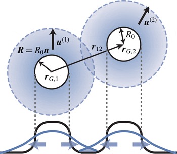
Next, we consider the interaction between two drops due to overlap of the concentration field. We follow the approach in Ohta et al. (Reference Ohta, Kiyose and Mimura1997), Ohta (Reference Ohta2001) (see figure 2). In Fourier space, (4.1) is
 $$\begin{eqnarray}\frac{\unicode[STIX]{x2202}c_{\boldsymbol{q}}}{\unicode[STIX]{x2202}t}=-D(q^{2}+\unicode[STIX]{x1D6FD}^{2})c_{\boldsymbol{ q}}+H_{\boldsymbol{q}},\end{eqnarray}$$
where the source term
 $H_{\boldsymbol{q}}$
is
 $$\begin{eqnarray}H_{\boldsymbol{q}}=A_{1}S_{q}^{(1)}\text{e}^{\text{i}\boldsymbol{q}\boldsymbol{\cdot }\boldsymbol{r}_{G,1}}+A_{2}S_{q}^{(2)}\text{e}^{\text{i}\boldsymbol{q}\boldsymbol{\cdot }\boldsymbol{r}_{G,2}}\end{eqnarray}$$
and
 $$\begin{eqnarray}S_{q}^{(1)}=S_{q}^{(2)}=S_{q}=4\unicode[STIX]{x03C0}\frac{\sin (qR_{0})-qR_{0}\cos (qR_{0})}{q^{3}}=\frac{4\unicode[STIX]{x03C0}R_{0}^{2}}{q}j_{1}(qR_{0}).\end{eqnarray}$$
The first term in (4.8) corresponds to the production of chemicals from the first drop (when
 $A_{1}>0$
) while the second term corresponds to production from the second drop (when
 $A_{2}>0$
). Here
 $j_{n}(x)$
for
 $n=0,1,2,\ldots$
are spherical Bessel functions, as defined in (A 2). As in Yabunaka et al. (Reference Yabunaka, Ohta and Yoshinaga2012), the solution of (4.7) is expanded close to the critical point of the drift bifurcation, that is, for
 $\unicode[STIX]{x1D716}=u/(D\unicode[STIX]{x1D6FD})\ll 1$
,
 $$\begin{eqnarray}c_{\boldsymbol{q}}=\frac{G_{q}}{D}H_{\boldsymbol{q}}-\frac{G_{q}^{2}}{D^{2}}\frac{\unicode[STIX]{x2202}H_{\boldsymbol{q}}}{\unicode[STIX]{x2202}t}+\frac{G_{q}^{3}}{D^{3}}\frac{\unicode[STIX]{x2202}^{2}H_{\boldsymbol{q}}}{\unicode[STIX]{x2202}t^{2}}-\frac{G_{q}^{4}}{D^{4}}\frac{\unicode[STIX]{x2202}^{3}H_{\boldsymbol{q}}}{\unicode[STIX]{x2202}t^{3}}+\cdots \,,\end{eqnarray}$$
where we use the Green’s function
 $$\begin{eqnarray}G_{q}=\frac{1}{q^{2}+\unicode[STIX]{x1D6FD}^{2}}.\end{eqnarray}$$
Note that the time derivative of
 $H_{\boldsymbol{q}}$
generate the velocity of the first or second drop (and their time derivative). After performing inverse Fourier transformation of (4.10), the concentration
 $c_{I}$
at the interface of the first drop can be expanded as
 $$\begin{eqnarray}c_{I}=c_{I}^{(0)}(\boldsymbol{r}_{G,1}+\boldsymbol{s})+c_{I}^{(1)}(\boldsymbol{r}_{G,1}+\boldsymbol{s})+c_{I}^{(2)}(\boldsymbol{r}_{G,1}+\boldsymbol{s})+c_{I}^{(3)}(\boldsymbol{r}_{G,1}+\boldsymbol{s})+\cdots \,.\end{eqnarray}$$
The lowest-order term in (4.12) can be explicitly written as
 $$\begin{eqnarray}\displaystyle c_{I}^{(0)}(\boldsymbol{r}_{G,1}+\boldsymbol{s}) & = & \displaystyle \frac{1}{D}\int _{\boldsymbol{q}}G_{q}[A_{1}S_{q}^{(1)}\text{e}^{\text{i}\boldsymbol{q}\boldsymbol{\cdot }\boldsymbol{r}_{G,1}}+A_{2}S_{q}^{(2)}\text{e}^{\text{i}\boldsymbol{q}\boldsymbol{\cdot }\boldsymbol{r}_{G,2}}]\text{e}^{-\text{i}\boldsymbol{q}\boldsymbol{\cdot }(\boldsymbol{r}_{G,1}+\boldsymbol{s})}\nonumber\\ \displaystyle & = & \displaystyle \frac{A_{1}}{D}[Q_{1}^{(0)}(s)+Q_{1}^{int}(\unicode[STIX]{x1D703},\unicode[STIX]{x1D711})],\end{eqnarray}$$
where the terms correspond to the respective terms in (4.8); the first term arises from self-production of the chemical concentration while the second term is from the interaction. The first term
 $Q_{n}^{(0)}(s)$
is
 $$\begin{eqnarray}\displaystyle Q_{n}^{(0)}(s) & = & \displaystyle \int _{\boldsymbol{q}}G_{q}^{n}S_{q}\text{e}^{-\text{i}\boldsymbol{q}\boldsymbol{\cdot }\boldsymbol{s}}\nonumber\\ \displaystyle & = & \displaystyle \frac{2{R_{0}}^{2}}{\unicode[STIX]{x03C0}}\int _{0}^{\infty }\text{d}q\,G_{q}^{n}qj_{1}(qR_{0})j_{0}(qs).\end{eqnarray}$$
There is no angular dependence, and thus this term describes an isotropic concentration field. Without hydrodynamic flow and the resulting motion of the drops, our model is isotropic, and therefore, the lowest-order concentration field must be isotropic. Nevertheless, as we will see, the coupling to the flow field or perturbation of the concentration field by another drop would result in an anisotropic concentration field, which would then lead to an inhomogeneous surface tension and self-propulsion. The contribution from interaction,
 $Q_{n}^{int}(\unicode[STIX]{x1D703},\unicode[STIX]{x1D711})$
in (4.13) can be calculated as
 $$\begin{eqnarray}\displaystyle Q_{n}^{int}(\boldsymbol{s}) & = & \displaystyle \frac{A_{2}}{A_{1}}\int _{\boldsymbol{q}}G_{q}S_{q}\text{e}^{-\text{i}\boldsymbol{q}\boldsymbol{\cdot }(\boldsymbol{s}+\boldsymbol{r}_{G,1}-\boldsymbol{r}_{G,2})}\nonumber\\ \displaystyle & = & \displaystyle \frac{2{R_{0}}^{2}A_{2}}{\unicode[STIX]{x03C0}A_{1}}\int _{0}^{\infty }\,\text{d}q\,G_{q}^{n}qj_{0}(q|\boldsymbol{s}+\boldsymbol{r}_{G,1}-\boldsymbol{r}_{G,2}|)j_{1}(qR_{0}).\end{eqnarray}$$
Using the addition theorem of spherical Bessel functions (Watson Reference Watson1922), we have
 $$\begin{eqnarray}\displaystyle j_{0}(q|\boldsymbol{s}+\boldsymbol{r}_{G,1}-\boldsymbol{r}_{G,2}|)=\mathop{\sum }_{l=0}^{\infty }(2l+1)j_{l}(qs)j_{l}(qr_{12})P_{l}(\cos \unicode[STIX]{x1D719}_{s12}), & & \displaystyle\end{eqnarray}$$
where
 $r_{12}=|\boldsymbol{r}_{G,2}-\boldsymbol{r}_{G,1}|$
and
 $\unicode[STIX]{x1D719}_{s12}$
is the angle between
 $\boldsymbol{s}$
and
 $\boldsymbol{r}_{12}=\boldsymbol{r}_{G,2}-\boldsymbol{r}_{G,1}$
. The Legendre polynomial can be decomposed as follows (Arfken, Weber & Weber Reference Arfken, Weber and Weber1968):
 $$\begin{eqnarray}P_{l}(\cos \unicode[STIX]{x1D719}_{s12})=\frac{4\unicode[STIX]{x03C0}}{2l+1}\mathop{\sum }_{m=-l}^{l}Y_{l}^{m}(\unicode[STIX]{x1D703},\unicode[STIX]{x1D711})Y_{l}^{m\ast }(\unicode[STIX]{x1D703}_{12},\unicode[STIX]{x1D711}_{12}).\end{eqnarray}$$
Then (4.15) becomes
 $$\begin{eqnarray}Q_{n}^{int}(\boldsymbol{s})=\frac{8{R_{0}}^{2}A_{2}}{A_{1}}\mathop{\sum }_{l=0}^{\infty }\mathop{\sum }_{m=-l}^{l}\int _{0}^{\infty }\,\text{d}q\,G_{q}^{n}qj_{1}(qR_{0})j_{l}(qs)j_{l}(qr_{12})Y_{l}^{m}(\unicode[STIX]{x1D703},\unicode[STIX]{x1D711})Y_{l}^{m\ast }(\unicode[STIX]{x1D703}_{12},\unicode[STIX]{x1D711}_{12}).\end{eqnarray}$$
This concentration field, (4.13) and (4.18), becomes anisotropic, since it contains
 $Y_{l}^{m}(\unicode[STIX]{x1D703},\unicode[STIX]{x1D711})$
. This arises from the coupling of the relative position
 $Y_{l}^{m\ast }(\unicode[STIX]{x1D703}_{12},\unicode[STIX]{x1D711}_{12})$
to the concentration field created by another drop in contrast with the isotropic term of (4.15).
In expansion of the concentration field, (4.12), the next-order term is
 $$\begin{eqnarray}\displaystyle c_{I}^{(1)}(\boldsymbol{r}_{G}+\boldsymbol{s}) & = & \displaystyle -\frac{A_{1}}{D^{2}}\int _{\boldsymbol{q}}G_{q}^{2}\left[(\text{i}\boldsymbol{q}\boldsymbol{\cdot }\boldsymbol{u}^{(1)})S_{q}^{(1)}\text{e}^{\text{i}\boldsymbol{q}\boldsymbol{\cdot }\boldsymbol{r}_{G,1}}+\frac{A_{2}}{A_{1}}(\text{i}\boldsymbol{q}\boldsymbol{\cdot }\boldsymbol{u}^{(2)})S_{q}^{(2)}\text{e}^{\text{i}\boldsymbol{q}\boldsymbol{\cdot }\boldsymbol{r}_{G,2}}\right]\text{e}^{-\text{i}\boldsymbol{q}\boldsymbol{\cdot }(\boldsymbol{r}_{G}+\boldsymbol{s})}\nonumber\\ \displaystyle & = & \displaystyle u_{i}^{(1)}\frac{A_{1}}{D^{2}}\left[n_{i}^{(0)}\frac{\unicode[STIX]{x2202}Q_{2}^{(0)}}{\unicode[STIX]{x2202}s}\right]+u_{i}^{(2)}\frac{A_{2}}{D^{2}}\frac{\unicode[STIX]{x2202}}{\unicode[STIX]{x2202}s_{i}}Q_{2}^{int},\end{eqnarray}$$
where the first term arises from the source term of the first drop and thus is the same as the velocity without the second drop. In contrast with the lowest-order concentration
 $c_{I}^{(0)}$
, both of the terms in (4.19) are anisotropic. In the first term, this is because the coupling to the velocity of the drop (
 $\boldsymbol{u}^{(1)}$
) and the concentration field. Since the drop is moving, the produced concentration field remains at the back of the drop, leading different concentrations between at the front and rear (Yabunaka et al.
Reference Yabunaka, Ohta and Yoshinaga2012). In the second term, both the velocity of the drop and the interaction produce an anisotropic concentration.
The velocity in (4.3) is expressed by the sum of the velocity due to the normal and tangential forces in (3.9) on the surface of the drop. Each force is the sum of the force for an isolated drop and the contribution from the interaction:
 $$\begin{eqnarray}\boldsymbol{u}_{0}+\boldsymbol{u}_{c}=\boldsymbol{u}_{1}+\boldsymbol{u}_{2},\end{eqnarray}$$
where
 $\boldsymbol{u}_{1}$
and
 $\boldsymbol{u}_{2}$
are the contributions from the normal and tangential forces, respectively. The velocities can be decomposed as follows:
 $$\begin{eqnarray}\displaystyle & \displaystyle \boldsymbol{u}_{1}=\boldsymbol{u}_{1}^{(0)}+\boldsymbol{u}_{1}^{int} & \displaystyle\end{eqnarray}$$
 $$\begin{eqnarray}\displaystyle & \displaystyle \boldsymbol{u}_{2}=\boldsymbol{u}_{2}^{(0)}+\boldsymbol{u}_{2}^{int}. & \displaystyle\end{eqnarray}$$
The Stokes equation (3.9) is solved by using the Oseen tensor,
 $$\begin{eqnarray}\unicode[STIX]{x1D61B}_{ij}=\frac{1}{8\unicode[STIX]{x03C0}\unicode[STIX]{x1D702}}\left[\frac{1}{r}\unicode[STIX]{x1D6FF}_{ij}+\frac{x_{i}x_{j}}{r^{3}}\right]\end{eqnarray}$$
and the interaction can be expanded with respect to the magnitude of the velocity of the second drop corresponding to each order in the expansion of (4.12):
 $\boldsymbol{u}_{1}^{int}=\boldsymbol{u}_{1}^{int,0}+\boldsymbol{u}_{1}^{int,1}+\boldsymbol{u}_{1}^{int,2}+\cdots \,.$
The lowest-order contribution from the interaction between spherical drops to the velocity is obtained from (4.13) and (4.18):
 $$\begin{eqnarray}\displaystyle u_{i,1}^{int,0} & = & \displaystyle \frac{\unicode[STIX]{x1D6FE}_{c}R_{0}}{\unicode[STIX]{x1D6FA}}\int \text{d}a\int \text{d}a^{\prime }n_{i}(a)\unicode[STIX]{x1D61B}_{jk}(a,a^{\prime })n_{j}(a)n_{k}(a^{\prime })\left(-\frac{2}{R_{0}}\right)c_{I}^{(0)}(a^{\prime })\nonumber\\ \displaystyle & = & \displaystyle -\frac{64\unicode[STIX]{x1D6FE}_{c}{R_{0}}^{2}A_{2}a_{1,0}^{(1)}}{15\unicode[STIX]{x1D702}D}\int _{0}^{\infty }\text{d}q\,qG_{q}j_{1}(qR_{0})j_{1}(qr_{12})j_{1}(qR_{0})N_{i}(\unicode[STIX]{x1D703}_{12},\unicode[STIX]{x1D711}_{12}),\end{eqnarray}$$
where
 $a_{1,0}^{(1)}=3/(4\unicode[STIX]{x03C0})$
and
 $$\begin{eqnarray}\boldsymbol{N}(\unicode[STIX]{x1D703}_{12},\unicode[STIX]{x1D711}_{12})=\hat{\boldsymbol{r}}_{12}=\frac{\boldsymbol{r}_{12}}{|\boldsymbol{r}_{12}|}=\frac{\boldsymbol{r}_{2,G}-\boldsymbol{r}_{1,G}}{|\boldsymbol{r}_{2,G}-\boldsymbol{r}_{1,G}|}\end{eqnarray}$$
is the normal vector pointing the second drop from the first drop. The velocity due to the tangential force is
 $$\begin{eqnarray}\displaystyle u_{i,2}^{int,0} & = & \displaystyle \frac{\unicode[STIX]{x1D6FE}_{c}R_{0}}{\unicode[STIX]{x1D6FA}}\int \text{d}a\int \text{d}a^{\prime }n_{i}(a)\unicode[STIX]{x1D61B}_{jk}(a,a^{\prime })n_{j}(a)[\unicode[STIX]{x1D6FF}_{kl}-n_{k}(a^{\prime })n_{l}(a^{\prime })]\unicode[STIX]{x1D735}_{l}c_{I}^{(0)}\nonumber\\ \displaystyle & = & \displaystyle \frac{\unicode[STIX]{x1D6FE}_{c}R_{0}^{2}}{5\unicode[STIX]{x1D6FA}\unicode[STIX]{x1D702}}\int \text{d}a^{\prime }[\unicode[STIX]{x1D6FF}_{ij}-n_{i}(a^{\prime })n_{j}(a^{\prime })]\unicode[STIX]{x1D735}_{j}c_{I}^{(0)}(a^{\prime }).\end{eqnarray}$$
In (4.13), the first contribution, which comes from
 $Q_{1}^{(0)}(s)$
, vanishes since
 $(\unicode[STIX]{x1D6FF}_{ij}-n_{i}(a^{\prime })n_{j}(a^{\prime }))n_{j}=0$
. This is obvious since the concentration field in (4.14) is isotropic. The second contribution comes from
 $Q_{1}^{\text{int}}(\unicode[STIX]{x1D703},\unicode[STIX]{x1D711})$
in (4.13) and is given by
 $$\begin{eqnarray}u_{i,2}^{int,0}=\frac{8\unicode[STIX]{x1D6FE}_{c}R_{0}^{3}A_{2}a_{0,1}^{(1)}}{5\unicode[STIX]{x1D702}D}\int _{0}^{\infty }\text{d}q\,qG_{q}j_{1}(qR_{0})j_{1}(qr_{12})j_{1}(qR_{0})N_{i}(\unicode[STIX]{x1D703}_{12},\unicode[STIX]{x1D711}_{12}),\end{eqnarray}$$
where
 $a_{0,1}^{(1)}=(2/R_{0})a_{1,0}^{(1)}$
. Both (4.24) and (4.27) are along the direction of the centreline between the two drops. This originates from the anisotropic concentration field created by the isotropic field around the other drop. Combining (4.24) and (4.27), we obtain
 $$\begin{eqnarray}\displaystyle \boldsymbol{u}_{c} & = & \displaystyle -\unicode[STIX]{x1D735}_{r_{1}}U_{0}(r_{12})\nonumber\\ \displaystyle & = & \displaystyle -\frac{\unicode[STIX]{x1D6FE}_{c}A_{2}}{\unicode[STIX]{x1D702}D\unicode[STIX]{x1D6FD}^{2}}k_{1}(\unicode[STIX]{x1D6FD}r_{12})g_{0}(\unicode[STIX]{x1D6FD}R_{0})\frac{\boldsymbol{r}_{2}-\boldsymbol{r}_{1}}{|\boldsymbol{r}_{2}-\boldsymbol{r}_{1}|},\end{eqnarray}$$
where
 $k_{n}(x)$
is the modified spherical Bessel function of the second kind, defined as
 $k_{n}=(-1)^{n}x^{n}(\text{d}/(x\,\text{d}x))^{n}(\exp (-x)/x)$
. The interaction may be expressed as if there is the following potential:
 $$\begin{eqnarray}U_{0}(r_{12})=\frac{16a_{1,0}^{(1)}\unicode[STIX]{x1D6FE}_{c}R_{0}^{2}A_{2}}{15\unicode[STIX]{x1D702}D}\int _{0}^{\infty }\,\text{d}q\,G_{q}j_{1}(qR_{0})j_{0}(qr_{12})j_{1}(qR_{0}).\end{eqnarray}$$
Here we have used (A 4). Using (A 5) and (A 7), we obtain
 $$\begin{eqnarray}U_{0}(r_{12})=\frac{\unicode[STIX]{x1D6FE}_{c}A_{2}}{\unicode[STIX]{x1D702}D\unicode[STIX]{x1D6FD}^{3}}g_{0}(\hat{R}_{0})k_{0}(\unicode[STIX]{x1D6FD}r_{12}),\end{eqnarray}$$
with
 $\hat{R}_{0}=\unicode[STIX]{x1D6FD}R_{0}$
. For given parameters, the potential decays exponentially at large distance between the two drops as
 $U_{0}=\tilde{U} _{0}k_{0}(\unicode[STIX]{x1D6FD}r_{12})$
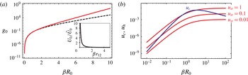
as shown figure 3(a). The magnitude of the potential
 $\tilde{U} _{0}=\unicode[STIX]{x1D6FE}_{c}A_{2}/(\unicode[STIX]{x1D702}D\unicode[STIX]{x1D6FD}^{3})g_{0}(\hat{R}_{0})$
depends on the parameters and the size of the drop. The size dependence is explicitly given by
 $$\begin{eqnarray}g_{0}(\hat{R}_{0})=-\frac{2a_{1,0}^{(1)}\unicode[STIX]{x03C0}}{15\hat{R}_{0}^{2}}[-2(\hat{R}_{0}^{2}+2)\cosh (2\hat{R}_{0})+5\hat{R}_{0}\sinh (2\hat{R}_{0})+4].\end{eqnarray}$$
The plot of
 $g_{0}$
is shown in figure 3. From (3.14), the activity of the first drop is controlled by
 $\unicode[STIX]{x1D6FE}_{c}A_{1}$
. In order to exhibit the instability for an isolated drop, the activity
 $\unicode[STIX]{x1D6FE}_{c}A_{1}$
must be positive. In that case, the inequality
 $g_{0}(\hat{R}_{0})\geqslant 0$
implies that the potential is repulsive when
 $A_{1}A_{2}>0$
and attractive when
 $A_{1}A_{2}<0$
.
4.3 Far-field approximation
When the distance between two drops is significantly larger than the size of the drops and the scaled radius is very small, we may simplify the calculation of the previous section. For
 $r_{12}\gg R_{0}$
, we have the following approximation
 $$\begin{eqnarray}\displaystyle |\boldsymbol{s}-\boldsymbol{r}_{12}|=r_{12}\left[1+\frac{s^{2}}{r_{12}^{2}}-\frac{2\boldsymbol{s}\boldsymbol{\cdot }\boldsymbol{r}_{12}}{r_{12}^{2}}\right]^{1/2}\simeq r_{12}\left[1-\frac{\boldsymbol{s}\boldsymbol{\cdot }\boldsymbol{r}_{12}}{r_{12}^{2}}+\left(\frac{s^{2}}{2r_{12}^{2}}-\frac{(\boldsymbol{s}\boldsymbol{\cdot }\boldsymbol{r}_{12})^{2}}{2r_{12}^{4}}\right)+\cdots \,\right]. & & \displaystyle \nonumber\\ \displaystyle & & \displaystyle\end{eqnarray}$$
Instead of using (4.16), for
 $\unicode[STIX]{x1D6FD}R_{0}\ll 1$
, we may use the following expansion:
 $$\begin{eqnarray}\displaystyle & & \displaystyle j_{0}(q|\boldsymbol{s}-\boldsymbol{r}_{12}|)\simeq j_{0}(qr_{12})-qr_{12}j_{0}^{\prime }(qr_{12})\frac{\boldsymbol{s}\boldsymbol{\cdot }\boldsymbol{r}_{12}}{r_{12}^{2}}\nonumber\\ \displaystyle & & \displaystyle \quad +\,\frac{qr_{12}}{2}\left[j_{0}^{\prime }(qr_{12})\frac{s^{2}}{r_{12}^{2}}+(-j_{0}^{\prime }(qr_{12})+qr_{12}j_{0}^{\prime \prime }(qr_{12}))\frac{(\boldsymbol{s}\boldsymbol{\cdot }\boldsymbol{r}_{12})^{2}}{r_{12}^{4}}\right]+\cdots \,.\end{eqnarray}$$
With this expansion, we will use (4.15) instead of (4.18). If we take only the zeroth-order term in the expansion of the concentration field, the velocity of the drop due to the normal force becomes
 $$\begin{eqnarray}u_{i,1}^{int,0}=-\frac{16R_{0}^{3}\unicode[STIX]{x1D6FE}_{c}A_{2}}{15\unicode[STIX]{x03C0}\unicode[STIX]{x1D6FA}\unicode[STIX]{x1D702}D}\int \text{d}a^{\prime }n_{i}^{(0)}(a^{\prime })\int \text{d}q\,G_{q}qj_{0}(q|\boldsymbol{R}(a^{\prime })-\boldsymbol{r}_{12}|)j_{1}(qR_{0}).\end{eqnarray}$$
For the spherical drop,
 $\boldsymbol{R}(a^{\prime })=R_{0}\boldsymbol{n}(a^{\prime })$
, and therefore, in (4.33), the terms which contain an even number of
 $\boldsymbol{s}$
do not contribute to the integral. The isotropic term in (4.33) does not make a contribution for
 $c_{I}^{(0)}$
. For the lowest-order approximation, the velocity becomes
 $$\begin{eqnarray}u_{i,1}^{int,0}\simeq -\frac{16R_{0}^{2}\unicode[STIX]{x1D6FE}_{c}A_{2}}{15\unicode[STIX]{x03C0}\unicode[STIX]{x1D702}D}N_{i}(\unicode[STIX]{x1D703}_{12},\unicode[STIX]{x1D711}_{12})\int \text{d}q\,G_{q}q^{2}R_{0}j_{1}(qr_{12})j_{1}(qR_{0}).\end{eqnarray}$$
The contribution from the tangential force is
 $$\begin{eqnarray}\displaystyle u_{i,2}^{int,0} & = & \displaystyle \frac{\unicode[STIX]{x1D6FE}_{c}R_{0}^{2}A_{1}}{5\unicode[STIX]{x1D6FA}\unicode[STIX]{x1D702}D}\int \text{d}a^{\prime }[\unicode[STIX]{x1D6FF}_{ij}-n_{i}^{(0)}(a^{\prime })n_{j}^{(0)}(a^{\prime })]\unicode[STIX]{x1D735}_{j}Q_{1}^{int}\nonumber\\ \displaystyle & = & \displaystyle \frac{4\unicode[STIX]{x1D6FE}_{c}R_{0}^{3}A_{2}}{5\unicode[STIX]{x03C0}\unicode[STIX]{x1D702}D}N_{j}(\unicode[STIX]{x1D703}_{12},\unicode[STIX]{x1D711}_{12})\int \text{d}q\,G_{q}q^{2}j_{1}(qR_{0})j_{1}(qr_{12}).\end{eqnarray}$$
Under the far-field approximation, we obtain the interaction
 $\boldsymbol{u}_{c}\sim k_{1}(\unicode[STIX]{x1D6FD}r_{12})\boldsymbol{N}$
, which is similar to that of (4.28), and the potential
 $U_{0}\sim k_{0}(\unicode[STIX]{x1D6FD}r_{12})$
, which is similar to that of (4.30), although we have a different functional form for
 $g_{0}(\unicode[STIX]{x1D6FD}R_{0})$
. Figure 3(a) shows
 $g_{0}(\unicode[STIX]{x1D6FD}R_{0})$
in (4.28) and that obtained under the far-field approximation. When
 $\unicode[STIX]{x1D6FD}R_{0}\ll 1$
, the two results agree, although they deviate when
 $\unicode[STIX]{x1D6FD}R_{0}\gg 1$
, since in that case, the far-field expansion is not justified.
We can analytically confirm that (4.28) approaches the above expression of
 $u_{i}^{\text{int},0}$
in the far-field limit
 $r_{12}\gg R_{0}$
and
 $\unicode[STIX]{x1D6FD}R_{0}\ll 1$
, by using the following relation, which holds in the far-field limit:
 $$\begin{eqnarray}\displaystyle 3\int \text{d}q\,qG_{q}(j_{1}(qR_{0}))^{2}j_{1}(qr_{12}) & \simeq & \displaystyle R_{0}\int \text{d}q\,q^{2}G_{q}j_{1}(qR_{0})j_{1}(qr_{12}).\end{eqnarray}$$
We can systematically compute the terms that are higher order with respect to the magnitude of the velocity of the second drop. For the first-order term in the expansion, the velocity is expressed as
 $$\begin{eqnarray}u_{i,1}^{int,1}=-\frac{8R_{0}\unicode[STIX]{x1D6FE}_{c}A_{2}}{15\unicode[STIX]{x1D6FA}\unicode[STIX]{x1D702}D^{2}}u_{j}^{(2)}\int \text{d}a^{\prime }n_{i}^{(0)}(a^{\prime })\frac{\unicode[STIX]{x2202}}{\unicode[STIX]{x2202}s_{j}}Q_{2}^{int}.\end{eqnarray}$$
Similarly, the other higher-order terms in the expansion contain higher derivatives with respect to
 $s_{i}$
. At the far-field limit, the first term in (4.33) does not depend on
 $s_{i}$
and therefore, in the higher-order terms, the gradient with respect to
 $s_{i}$
vanishes. At the next order,
 $Q_{n}^{int}$
is linear in
 $\boldsymbol{s}$
and therefore the higher-order terms do not contribute to the velocity. The higher-order terms start to appear beginning with the third term in (4.33). The same argument can also be applied to the tangential force. From the symmetry, this term should vanish for the second term in (4.33). Indeed, the integral has an odd number of normal vectors and thus it vanishes. We note that although we have considered only a spherical drop, in the general case, the shape of the first drop may affect its velocity. Consequently, the interaction cannot be expressed in the simple form as a potential, as in (4.28).
5 Collision of two particles
In the previous sections, we have discussed two-body interactions. The results give kinetic rules for the position (
 $\boldsymbol{x}^{(\unicode[STIX]{x1D6FC})}$
) and velocity (
 $\boldsymbol{u}^{(\unicode[STIX]{x1D6FC})}$
) of the
 $\unicode[STIX]{x1D6FC}$
th drop (
 $\unicode[STIX]{x1D6FC}=1,2$
). We assume there is no viscosity contrast, that is,
 $\unicode[STIX]{x1D702}^{(o)}=\unicode[STIX]{x1D702}^{(i)}$
. The kinetic equations are
 $$\begin{eqnarray}\displaystyle & \displaystyle \frac{\text{d}\boldsymbol{x}^{(1)}}{\text{d}t}=\boldsymbol{u}^{(1)} & \displaystyle\end{eqnarray}$$
 $$\begin{eqnarray}\displaystyle & \displaystyle m\frac{\text{d}\boldsymbol{u}^{(1)}}{\text{d}t}=(\unicode[STIX]{x1D70F}-\unicode[STIX]{x1D70F}_{c})\boldsymbol{u}^{(1)}-g|\boldsymbol{u}^{(1)}|^{2}\boldsymbol{u}^{(1)}+\unicode[STIX]{x1D70F}_{c}(\boldsymbol{u}_{c}+\boldsymbol{u}_{h}), & \displaystyle\end{eqnarray}$$
where
 $\!$
the interactions due to concentration overlap
 $\!$
and hydrodynamics are,
 $\!$
respectively,
 $$\begin{eqnarray}\displaystyle & \displaystyle \boldsymbol{u}_{c}=-\unicode[STIX]{x1D735}_{\boldsymbol{r}_{1}}U_{0}(r_{12})=-\frac{\unicode[STIX]{x1D6FE}_{c}A_{2}}{\unicode[STIX]{x1D702}D\unicode[STIX]{x1D6FD}^{2}}g_{0}(\unicode[STIX]{x1D6FD}R_{0})k_{1}(\unicode[STIX]{x1D6FD}r_{12})\boldsymbol{N} & \displaystyle\end{eqnarray}$$
 $$\begin{eqnarray}\displaystyle & \displaystyle \boldsymbol{u}_{h}=\left(\frac{R}{r_{12}}\right)^{3}\left[-\frac{1}{2}\unicode[STIX]{x1D6FF}_{ij}+\frac{3}{2}\boldsymbol{N}\boldsymbol{N}\right]\boldsymbol{\cdot }\boldsymbol{u}^{(2)}+O\left(\left(\frac{R}{r_{12}}\right)^{2}\boldsymbol{S}^{(2)}\boldsymbol{\cdot }\boldsymbol{N}\right), & \displaystyle\end{eqnarray}$$
where the directional vector is from the first drop and points toward the second drop (4.25). The coefficients
 $m$
,
 $\unicode[STIX]{x1D70F}$
and
 $g$
are found in Yabunaka et al. (Reference Yabunaka, Ohta and Yoshinaga2012). Note that (5.2) is an equation for velocity since the effective mass
 $m$
has the dimension of time. The equation of motion for the second drop is obtained by interchanging the indices
 $1\leftrightarrow 2$
.
 $S_{ij}$
is the dipolar concentration distribution created around the drop,
 $S_{ij}=(R_{0}/\unicode[STIX]{x1D6FA})\int [n_{i}(a)n_{j}(a)-(1/3)\unicode[STIX]{x1D6FF}_{ij}]c(a)\,\text{d}a$
. This second moment of the concentration field arises both from ellipsoidal deformation and self-propulsion (Yoshinaga Reference Yoshinaga2014). Since we consider a spherical drop and assume the system is close to the drift bifurcation point,
 $S_{ij}\sim \unicode[STIX]{x1D716}^{2}$
, the contribution of the second term in (5.4) is negligible.
The sign of the coefficients is
 $-(\unicode[STIX]{x1D6FE}_{c}A_{2})/(\unicode[STIX]{x1D702}D\unicode[STIX]{x1D6FD}^{2})g_{0}(\unicode[STIX]{x1D6FD}R_{0})k_{1}(\unicode[STIX]{x1D6FD}r_{12})<0$
when
 $\unicode[STIX]{x1D6FE}_{c}A_{2}>0$
. From (3.14) and (4.31), the self-propelled first drop (above the drift bifurcation) feels the interaction potential created by the second drop. The two drops repel each other when both produce or both consume chemicals. When the chemical reactions of the two drops have opposite signs, the interaction has the opposite sign and the two drops are mutually attracted. The interaction decays exponentially, as shown in figure 3(a). As the size of the drop increases, the concentration gradient associated with the concentration-mediated interaction becomes stronger at the fixed position. When the two drops approach, the interaction is best evaluated at
 $\unicode[STIX]{x1D6FD}^{-1}$
, which is outside the interface of the drops. For a larger drop, the concentration field is strongly screened, and the interaction becomes weaker. Therefore, the concentration-mediated interaction
 $u_{c}$
is most effective at
 $\unicode[STIX]{x1D6FD}R_{0}\simeq 1$
. In figure 3(b), the hydrodynamic interaction
 $\boldsymbol{u}_{h}$
evaluated at the distance of the characteristic length
 $r_{12}=2R_{0}+\unicode[STIX]{x1D6FD}^{-1}$
is shown for different values of the steady velocity. This distance corresponds to the situation in which the gap between the two drops is
 $\unicode[STIX]{x1D6FD}^{-1}$
. As the system gets closer to the critical point, the steady velocity decreases, and the hydrodynamic interaction becomes weaker. On the other hand, the leading order of the interaction mediated by the concentration is independent from the steady velocity. Therefore, near the critical point, the interaction is dominated by the concentration field and not by the hydrodynamic interaction.
For a head-on collision, the relative position
 $\unicode[STIX]{x1D709}=z^{(1)}-z^{(2)}$
between the two drops is obtained from (5.1) and (5.2):
 $$\begin{eqnarray}m\ddot{\unicode[STIX]{x1D709}}=\dot{\unicode[STIX]{x1D709}}\left(\unicode[STIX]{x1D70F}-\unicode[STIX]{x1D70F}_{c}-\frac{g}{4}\dot{\unicode[STIX]{x1D709}}^{2}\right)-\unicode[STIX]{x1D70F}_{c}\left(2U_{0}^{\prime }(\unicode[STIX]{x1D709})+\left(\frac{R}{\unicode[STIX]{x1D709}}\right)^{3}\dot{\unicode[STIX]{x1D709}}\right),\end{eqnarray}$$
where
 $\dot{\unicode[STIX]{x1D709}}=\text{d}\unicode[STIX]{x1D709}/\text{d}t$
. The hydrodynamic interaction is repulsive before the collision. However, after the collision, and when the two drops move away from each other, the interaction becomes attractive. This contrasts with the behaviour seen in an isotropic concentration-mediated interaction. Near the critical point, the steady velocity of a drop is small, and thus the interaction created by the concentration field is stronger than that created by the hydrodynamics. Trajectories and velocity of the solution of (5.5) are shown in § 7 together with the numerical results. Although the assumptions that we have made in the calculation of the interactions are not completely justified especially during collision, we will show in the following sections that this is in semi-quantitative agreement with our numerical results.
When the motion of two drops is confined in the
 $xz$
-plane, and the collision has a symmetry with respect to the
 $x$
-axis, the dynamics is expressed by
 $\unicode[STIX]{x1D709}=z^{(1)}-z^{(2)}$
and
 $\unicode[STIX]{x1D70C}=x^{(1)}+x^{(2)}$
, as follows:
 $$\begin{eqnarray}\displaystyle & \displaystyle m\ddot{\unicode[STIX]{x1D709}}=\dot{\unicode[STIX]{x1D709}}\left(\unicode[STIX]{x1D70F}-\unicode[STIX]{x1D70F}_{c}-\frac{g}{4}(\dot{\unicode[STIX]{x1D709}}^{2}+\dot{\unicode[STIX]{x1D70C}}^{2})\right)-\unicode[STIX]{x1D70F}_{c}\left(2U_{0}^{\prime }(\unicode[STIX]{x1D709})+\left(\frac{R}{\unicode[STIX]{x1D709}}\right)^{3}\dot{\unicode[STIX]{x1D709}}\right) & \displaystyle\end{eqnarray}$$
 $$\begin{eqnarray}\displaystyle & \displaystyle m\ddot{\unicode[STIX]{x1D70C}}=\dot{\unicode[STIX]{x1D70C}}\left(\unicode[STIX]{x1D70F}-\unicode[STIX]{x1D70F}_{c}-\frac{g}{4}(\dot{\unicode[STIX]{x1D709}}^{2}+\dot{\unicode[STIX]{x1D70C}}^{2})\right)-\frac{\unicode[STIX]{x1D70F}_{c}}{2}\left(\frac{R}{\unicode[STIX]{x1D709}}\right)^{3}\dot{\unicode[STIX]{x1D70C}}. & \displaystyle\end{eqnarray}$$
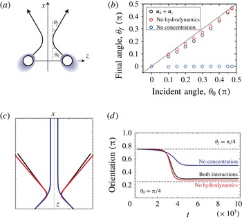
Two drops collide with an incident angle
 $\unicode[STIX]{x1D703}_{0}$
and a final angle
 $\unicode[STIX]{x1D703}_{f}$
(figure 4
a). Trajectories of the solution of (5.6) and (5.7) for
 $\unicode[STIX]{x1D703}_{0}=\unicode[STIX]{x03C0}/4$
are shown in figure 4(c). The parameters are chosen to be the same as the numerical simulations for
 $\unicode[STIX]{x1D702}=2.3$
. During the collision, the direction of motion changes from the incident angle,
 $\unicode[STIX]{x1D703}_{0}$
, and it reaches the final angle,
 $\unicode[STIX]{x1D703}_{f}$
(figure 4
d). The final angle is dependent on the incident angle, as shown in figure 4(b). When the incident angle is between
 $0$
and
 $\unicode[STIX]{x03C0}$
, the final angle is smaller than the incident angle. The hydrodynamic interaction enhances this effect; the final angle is less smaller than the incident angle if we eliminate the hydrodynamic interaction. On the other hand, if we eliminate the concentration-mediated interaction, two drops always align.
6 Numerical simulations: single drop
We numerically solve (3.2), which gives the dynamics of a drop and (3.9), which gives the flow field. We used the following equation for the dynamics of the concentration field similar to (4.1):
 $$\begin{eqnarray}\frac{\unicode[STIX]{x2202}c}{\unicode[STIX]{x2202}t}+\boldsymbol{v}\boldsymbol{\cdot }\unicode[STIX]{x1D735}c=D\unicode[STIX]{x1D6FB}^{2}c-\unicode[STIX]{x1D705}c+\frac{1}{2}A(\unicode[STIX]{x1D719}(\boldsymbol{r})+1).\end{eqnarray}$$
We assumed an axisymmetric system in which the motion of the drop was confined along the
 $z$
-axis. The entire space was discretized in cylindrical coordinates, with
 $N_{z}=96$
and
 $N_{r}=48$
mesh points in the
 $z$
- and radial (
 $r$
-) directions, respectively. The mesh size was chosen to be
 $\unicode[STIX]{x0394}z=\unicode[STIX]{x0394}r=1$
, and the time step was
 $\unicode[STIX]{x0394}t=0.002$
. Equations (6.1) and (3.2) were discretized by using the forward Euler method. We imposed a periodic boundary condition in the
 $z$
-direction, and, at
 $r=N_{r}$
, we imposed the slip boundary condition
 $\unicode[STIX]{x2202}_{r}v_{z}=0$
and
 $v_{r}=0$
, the non-wetting boundary condition
 $\unicode[STIX]{x2202}_{r}\unicode[STIX]{x1D719}=0$
, the no-flux boundary condition
 $\unicode[STIX]{x2202}_{r}(\unicode[STIX]{x1D6FF}f/\unicode[STIX]{x1D6FF}\unicode[STIX]{x1D719})=0$
, and
 $\unicode[STIX]{x2202}_{r}c=0$
. The Stokes equation was solved by using the relaxation method; for a given force
 $\boldsymbol{f}(\boldsymbol{r})$
, (3.9) was solved by introducing the virtual time derivative
 $\text{d}\boldsymbol{v}/\text{d}t$
and relaxing until a steady state was obtained. At each step in the virtual time domain, the pressure was relaxed to the steady value so that the incompressibility condition was satisfied. For the discretization, we employed the staggered lattice method, in which the
 $r$
and
 $z$
components of the flux were defined at the lattice points
 $((\text{i}+1/2)\unicode[STIX]{x0394}r,j\unicode[STIX]{x0394}z)$
and
 $(\text{i}\unicode[STIX]{x0394}r,(j+1/2)\unicode[STIX]{x0394}z)$
, respectively, for
 $i=0,\ldots ,N_{r}-1$
and
 $j=0,\ldots ,N_{z}-1$
. In order to quickly prepare initial conditions that are stationary under (6.1) and (3.2) with
 $\boldsymbol{v}=0$
, we solved the following equations
 $$\begin{eqnarray}\displaystyle & \displaystyle \frac{\unicode[STIX]{x2202}c}{\unicode[STIX]{x2202}t^{\prime }}=\unicode[STIX]{x1D6FC}\left[D\unicode[STIX]{x1D6FB}^{2}c-\unicode[STIX]{x1D705}c+\frac{1}{2}A(\unicode[STIX]{x1D719}(\boldsymbol{r})+1)\right], & \displaystyle\end{eqnarray}$$
 $$\begin{eqnarray}\displaystyle & \displaystyle \frac{\unicode[STIX]{x2202}\unicode[STIX]{x1D719}}{\unicode[STIX]{x2202}t^{\prime }}=-\frac{\unicode[STIX]{x1D6FF}F}{\unicode[STIX]{x1D6FF}\unicode[STIX]{x1D719}}+\left<\frac{\unicode[STIX]{x1D6FF}F}{\unicode[STIX]{x1D6FF}\unicode[STIX]{x1D719}}\right>, & \displaystyle\end{eqnarray}$$
with
 $\unicode[STIX]{x1D6FC}=20$
and
 $\unicode[STIX]{x0394}t^{\prime }=0.01$
until
 $t^{\prime }=160$
, starting from
 $c=0$
and
 $\unicode[STIX]{x1D719}=-\tanh (R-|\boldsymbol{r}-\boldsymbol{r}_{G,1}|)+0.05$
at
 $t^{\prime }=0$
. We added a small-amplitude noise to this initial condition in order to investigate the self-propelled motion of a drop with spontaneous symmetry breaking.
The flow field created by an isolated drop. (a) The
 $l=1$
mode associated with the translational motion under
 $\unicode[STIX]{x1D6FE}_{1,0}>0$
, as given by (2.15) and (2.16). The direction of motion is indicated by the thick arrow. (b) The
 $l=2$
mode of the dipolar flow for
 $\unicode[STIX]{x1D6FE}_{2,0}>0$
, as given by (2.19) and (2.20). The schematic drawings of the flow fields are also shown.

First, we dropped the advection term in (6.1) in order to directly compare our numerical results with the theoretical predictions of Yabunaka et al. (Reference Yabunaka, Ohta and Yoshinaga2012). We varied the viscosity
 $\unicode[STIX]{x1D702}$
to realize self-propulsive motion under fixed
 $R=16$
,
 $B_{0}=0.2$
,
 $B_{1}=0.5$
,
 $D=0.5$
,
 $A=0.08$
,
 $\unicode[STIX]{x1D705}=0.005$
and
 $L=1$
. Here
 $\unicode[STIX]{x1D6FD}=\sqrt{\unicode[STIX]{x1D705}/D}=0.1$
. We confirmed that this choice of parameters satisfies the assumptions listed following (3.10). With these parameters, the critical value of the viscosity is theoretically predicted as
 $\unicode[STIX]{x1D702}_{c}\simeq 1.742$
when using (3.14). We will discuss possible reasons for the discrepancies between the numerical results and the theoretical predictions in detail in § 7. In order to estimate the critical value, we need to evaluate the surface tension and
 $\unicode[STIX]{x1D6FE}_{c}$
. When the interface is sharp and the value of
 $c(\boldsymbol{r})$
at the interface is unique, then
 $\unicode[STIX]{x1D6FE}=(2\sqrt{2B(c)}/3)$
and
 $\unicode[STIX]{x1D6FE}_{c}=(\sqrt{2}B_{1}/3\sqrt{B(c)})$
. However, since we use a diffuse-interface model, the concentration at the interface region varies in space. The surface tension is
 $$\begin{eqnarray}\unicode[STIX]{x1D6FE}=\int B(c)\left(\frac{\unicode[STIX]{x2202}\unicode[STIX]{x1D719}}{\unicode[STIX]{x2202}n}\right)^{2}\,\text{d}n,\end{eqnarray}$$
where
 $\unicode[STIX]{x2202}/\unicode[STIX]{x2202}n$
is the spatial derivative along the direction normal to the interface. We numerically estimated (6.4) and compared the results with (3.8) to obtain
 $\unicode[STIX]{x1D6FE}_{c}\sim 0.510$
.
When
 $\unicode[STIX]{x1D702}<\unicode[STIX]{x1D702}_{c}$
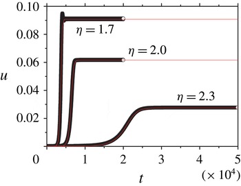
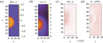
, the stationary state becomes unstable, and the drop starts to move. The velocity of the drop gradually increases until it reaches a steady state, as shown in figure 5. During the self-propulsive motion, the concentration field is distorted around the drop, as shown in figure 6. Clearly, the two centres of mass (that of the drop and that of the concentration) are shifted, and thus the symmetry is broken for the
 $\pm z$
directions. The velocity field during the motion is shown in figure 6. The velocity field in the drop frame shows a circular flow that corresponds to the
 $l=1$
mode in figure 1. Around the drop, the velocity field decays faster than
 $1/r$
, suggesting that the motion is generated by the source dipole and not by a Stokeslet.
When the viscosity
 $\unicode[STIX]{x1D702}$
is close to the critical value, the relaxation of the velocity is monotonic and well fitted with (3.17). This is consistent with the theoretical result of (3.15). When
 $\unicode[STIX]{x1D702}$
is much smaller than the critical value, however, the relaxation of the velocity is not monotonic but has a small oscillation, as seen for
 $\unicode[STIX]{x1D702}=1.7$
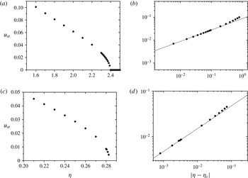
in figure 5. This may arise from the involvement of an additional time scale, and the truncation of the expansion of (4.10) is not completely satisfied. The steady velocity and the relaxation time are plotted in figure 7. As the viscosity
 $\unicode[STIX]{x1D702}$
decreases, that is, as
 $\unicode[STIX]{x1D70F}_{c}$
decreases, the self-propulsive speed increases. As suggested in figure 7(b,d), close to the critical point, the speed increases as
 $u\sim |\unicode[STIX]{x1D702}_{c}-\unicode[STIX]{x1D702}|^{1/2}$
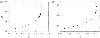
, which is predicted by the theory in (3.15). Figure 8 shows the relaxation time of the numerical simulations. As the viscosity approaches the critical value from below, the relaxation time diverges. This behaviour is also consistent with our theory in (3.17).
A schematic representation of interacting spherical drops. Each drop produces an outer concentration field. The black line shows the drop described by the field
 $\unicode[STIX]{x1D719}(\boldsymbol{r})$
. The blue (grey) lines indicate the concentration fields that are independently created by each drop. The total concentration field
 $c(\boldsymbol{r})$
contains the overlap between the two fields and the two drops interact through this field. At the bottom is a side view of the fields
 $\unicode[STIX]{x1D719}(\boldsymbol{r})$
and
 $c(\boldsymbol{r})$
.

(a) Semilogarithmic plot of the normalized concentration-mediated interaction as a function of the normalized size of the drop,
 $\unicode[STIX]{x1D6FD}R_{0}$
. The solid (red) line shows
 $g_{0}(\unicode[STIX]{x1D6FD}R_{0})$
, as in (4.28), and the dashed (black) line corresponds to the result under the far-field approximation. Inset: the interaction potential
 $U_{0}/\tilde{U} _{0}=k_{0}(\unicode[STIX]{x1D6FD}r_{12})$
as a function of the distance between the two drops when
 $A_{1}A_{2}>0$
. (b) Log–log plot of the typical hydrodynamic
 $u_{h}$
and concentration-mediated
 $u_{c}$
interactions for drops of different normalized sizes (
 $\unicode[STIX]{x1D6FD}R_{0}$
). The interactions are evaluated at the characteristic length scale
 $r_{12}=2R_{0}+\unicode[STIX]{x1D6FD}^{-1}$
. For the hydrodynamic interaction, the steady velocity of the second drop without interactions is decreased from the top to the bottom line.

(a) A schematic representation of a collision, (b) the incident,
 $\unicode[STIX]{x1D703}_{0}$
, and final,
 $\unicode[STIX]{x1D703}_{f}$
, angles for the solution of (5.6) and (5.7) (black), without the hydrodynamic interaction (red), and without the concentration-mediated interaction (blue), (c) the trajectories during the collisions for
 $\unicode[STIX]{x1D703}_{0}=\unicode[STIX]{x03C0}/4$
and (d) the direction of motion during the collisions for
 $\unicode[STIX]{x1D703}_{0}=\unicode[STIX]{x03C0}/4$
.

Self-propulsive velocity of a single drop. The velocity of the drop as a function of time is shown for numerical simulation (circles) and theory in (3.15) (line).

For a drop at steady state with
 $\unicode[STIX]{x1D702}=1.5$
and
 $t=3168$
: (a)
 $\unicode[STIX]{x1D719}(\boldsymbol{r})$
, (b) the concentration field
 $c(\boldsymbol{r})$
, and (c,d) the velocity field
 $\boldsymbol{v}(\boldsymbol{r})$
in the laboratory frame (c) and in the drop frame (d). The self-propulsive velocity is
 $u=0.109$
.

The steady velocity
 $u_{st}$
with varying viscosity
 $\unicode[STIX]{x1D702}$
(
 $\unicode[STIX]{x1D70F}_{c}$
). (a,b) Without advection of the third dilute component, and (c,d) with advection. The log–log plots of the steady velocity and the distance from the critical points are shown in (b) and (d). The solid lines show the exponent
 $u_{st}\sim |\unicode[STIX]{x1D702}-\unicode[STIX]{x1D702}_{c}|^{1/2}$
.

The relaxation time to reach the steady velocity. (a) Without advection of the third dilute component and (b) with advection. The vertical dashed lines correspond to the critical viscosity.

We evaluate the scaled coefficients
 $m$
,
 $\unicode[STIX]{x1D70F}$
and
 $g$
(
 $\hat{m},\hat{\unicode[STIX]{x1D70F}},{\hat{g}}$
in Yabunaka et al. (Reference Yabunaka, Ohta and Yoshinaga2012)) by comparison with the numerical results, as follows. In terms of the non-scaled coefficients
 $M$
,
 $T$
and
 $G$
(
 $m,\unicode[STIX]{x1D70F},g$
in Yabunaka et al. (Reference Yabunaka, Ohta and Yoshinaga2012)), the relaxation time and the steady velocity are expressed, respectively, as
 $$\begin{eqnarray}s_{r}=\frac{M}{T-1}\end{eqnarray}$$
 $$\begin{eqnarray}u_{st}=\sqrt{\frac{T-1}{G}}.\end{eqnarray}$$
Since
 $T\sim \unicode[STIX]{x1D702}^{-1}$
, the above expression for
 $s_{r}$
predicts the divergence of the relaxation time near the threshold, which is in agreement with the numerical results in figure 8. Using
 $\unicode[STIX]{x1D702}_{c}=2.395$
, we estimate
 $T-1\sim 0.19$
for
 $\unicode[STIX]{x1D702}=2.0$
. From the above equations, we estimate
 $G\sim 49.4$
and
 $M\sim 96.9$
. After rescaling the parameters of Yabunaka et al. (Reference Yabunaka, Ohta and Yoshinaga2012), we obtain
 $$\begin{eqnarray}\displaystyle & \displaystyle g=\unicode[STIX]{x1D70F}_{c}(D\unicode[STIX]{x1D6FD})^{2}G=0.0112, & \displaystyle\end{eqnarray}$$
 $$\begin{eqnarray}\displaystyle & \displaystyle m=MD\unicode[STIX]{x1D6FD}^{2}\unicode[STIX]{x1D70F}_{c}=0.044. & \displaystyle\end{eqnarray}$$
These values of
 $m$
and
 $g$
agree with the theoretical predictions in Yabunaka et al. (Reference Yabunaka, Ohta and Yoshinaga2012) with
 $\unicode[STIX]{x1D6FD}R=1.6$
. In the same way, we evaluated
 $g$
and
 $m$
for other values of
 $\unicode[STIX]{x1D702}$
near
 $\unicode[STIX]{x1D702}_{c}$
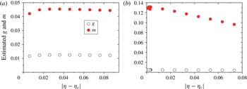
, as shown in figure 9. We found that they are almost constant, which is consistent with the theoretical predictions.
Numerically estimated coefficients
 $g$
and
 $m$
. (a) Without advection of the third dilute component, and (b) with advection.

The advection term in (6.1) does not change the qualitative features of the transition; we found that, when
 $\unicode[STIX]{x1D702}<\unicode[STIX]{x1D702}_{c}=0.2833$
, the stationary state becomes unstable, and the drop starts to move. In addition, figures 7 and 8 show that the advection does not modify the scaling behaviour of the steady velocity near the critical point. Both with and without the advection term, the steady velocity grows as
 $|\unicode[STIX]{x1D702}-\unicode[STIX]{x1D702}_{c}|^{1/2}$
. The relaxation time also diverges near the bifurcation point. We note that the critical point when there is advection (
 $\unicode[STIX]{x1D702}_{c}=0.2833$
) is much smaller than when there is no advection (
 $\unicode[STIX]{x1D702}_{c}=2.395$
). In Yabunaka et al. (Reference Yabunaka, Ohta and Yoshinaga2012), the effect of the advection is only treated in the limit
 $\unicode[STIX]{x1D6FD}R\rightarrow 0$
and it is predicted that, in the presence of advection, the drift instability is suppressed, but the bifurcation behaviour will not be essentially changed. Thus, our numerical results with
 $\unicode[STIX]{x1D6FD}R=1.6$
agree qualitatively with the theoretical prediction as
 $\unicode[STIX]{x1D6FD}R\rightarrow 0$
, even though the theory does not directly apply to our case.
7 Numerical simulations: interaction
With the same numerical method that we used in the previous section for an isolated drop, we carried out numerical simulations for two drops. The entire space was discretized in cylindrical coordinates with
 $N_{z}=200$
and
 $N_{r}=48$
mesh points in the
 $z$
- and radial (
 $r$
-) directions. The mesh size was chosen to be
 $\unicode[STIX]{x0394}z=\unicode[STIX]{x0394}r=1$
, and the time step was
 $\unicode[STIX]{x0394}t=0.002$
for
 $\unicode[STIX]{x1D702}>1.9$
and
 $\unicode[STIX]{x0394}t=0.001$
for
 $\unicode[STIX]{x1D702}<1.9$
. We prepared the initial condition in the same way, but with
 $\unicode[STIX]{x1D719}=\tanh (R-|\boldsymbol{r}-\boldsymbol{r}_{G,1}|)+\tanh (R-|\boldsymbol{r}-\boldsymbol{r}_{G,2}|)-2+0.05$
with
 $\boldsymbol{r}_{G,1}=29$
and
 $\boldsymbol{r}_{G,2}=171$
.
The trajectories of two colliding drops for (a)
 $\unicode[STIX]{x1D702}=1.5$
and (b)
 $\unicode[STIX]{x1D702}=2.3$
. The slices of the field
 $\unicode[STIX]{x1D719}$
at
 $r=0$
are superposed for the direction of time. The darker (brighter) region corresponds to
 $\unicode[STIX]{x1D719}=1$
(
 $\unicode[STIX]{x1D719}=-1$
). The solid lines show the trajectories of the centres of the drops. Because of the periodic boundary condition, the drops reaching the top or bottom boundaries are reflected by the interactions with image drops outside the simulation box.

Figure 10 shows the trajectory of the two centres of mass of the interacting particles. There are two distinct dynamics for the collision: fusion, as shown in figure 10(a), and reflection, as shown in figure 10(b). When the viscosity
 $\unicode[STIX]{x1D702}$
is far below the critical point, the two drops approach and eventually merge. On the other hand, when
 $\unicode[STIX]{x1D702}$
is close to the critical point, the two drops do not merge even when they are approaching, but they reflect and move in opposite directions. Surprisingly, the latter collision is elastic, despite the fact that the system is dissipative. The drops move at the same speed after the collision as they did before the collision. This can be understood from our reduced description (3.10), in which friction vanishes as
 $\unicode[STIX]{x1D70F}_{c}$
approaches
 $\unicode[STIX]{x1D70F}$
; note that
 $\unicode[STIX]{x1D70F}_{c}$
is proportional to
 $\unicode[STIX]{x1D702}$
as shown in (3.14). Thus, the drop behaves as if it were in a conserved system because of the balance between dissipation and the energy injection associated with chemical production. This is in contrast with both the squirmer and the Janus particle, since in those models, there is no inertia term in the equation of motion. We note that similar elastic behaviour has been reported for pulse collisions in reaction–diffusion systems (Ohta et al.
Reference Ohta, Kiyose and Mimura1997; Ei et al.
Reference Ei, Mimura and Nagayama2006).
In order to clarify the origin of the interaction, we solve the reduced equation (5.5), and compare with the full numerical simulations using the same initial conditions. The additional terms, which describe the interaction with image drops, are added to (5.5) in order to take into account the periodic boundary condition used in the simulation. The parameters in (5.5) are obtained from the result of a single drop, and thus there is no fitting parameter in the equation. The result for
 $\unicode[STIX]{x1D702}=2.3$
(figure 10
b) is shown in figure 11(a,b). There is good agreement between the results of the reduced equation and those of the original model. We found that the overall behaviour of the evolution of
 $\boldsymbol{u}$
is dominated by the concentration-mediated interaction, although the hydrodynamic interaction gives some correction on it. The contributions from the hydrodynamic (
 ${\sim}\unicode[STIX]{x1D709}^{-3}$
) and concentration-mediated interactions (
 ${\sim}U_{0}^{\prime }(\unicode[STIX]{x1D709})$
) are shown in figure 11. Over most of the region,
 $u_{c}$
dominates
 $u_{h}$
. However, the hydrodynamic interaction dominates when
 $\unicode[STIX]{x1D709}\gg 80$
, since the hydrodynamic (concentration-mediated) interaction decays algebraically (exponentially). For
 $\unicode[STIX]{x1D702}=1.5$
(figure 10
a), we solved (5.5), as shown in figure 11(d) and we found that
 $\unicode[STIX]{x1D709}$
becomes smaller than
 $2R$
, which suggests fusion of the drops and agrees with the results of the numerical simulation with the original model.
This result is consistent with the following rough estimate of the relative magnitudes of these two interactions: the magnitude of the hydrodynamic interaction is estimated to be
 $$\begin{eqnarray}|\boldsymbol{u}_{h}|=\left(\frac{R}{\unicode[STIX]{x1D709}}\right)^{3}u_{j}^{(2)}\sim u_{st}\left(\frac{R}{\unicode[STIX]{x1D709}}\right)^{3},\end{eqnarray}$$
where the typical self-propelling velocity in the steady state is given by
 $u_{st}\sim 0.02$
. The magnitude of the concentration-mediated interaction is
 $$\begin{eqnarray}|\boldsymbol{u}_{c}|\sim \frac{15D\unicode[STIX]{x1D6FD}}{2\unicode[STIX]{x1D70F}_{c}}g_{0}(\hat{R}_{0})k_{1}(\unicode[STIX]{x1D6FD}\unicode[STIX]{x1D709}),\end{eqnarray}$$
where
 $g_{0}(\hat{R}_{0}=1.6)\sim 0.39$
. If we set
 $\unicode[STIX]{x1D709}=2R$
and
 $k_{1}(\unicode[STIX]{x1D6FD}\unicode[STIX]{x1D709})\sim 0.0167$
, then
 $\boldsymbol{u}_{c}\sim 0.213$
and
 $\boldsymbol{u}_{h}\sim 0.0025$
. This also confirms that the magnitude of the concentration-overlap-mediated interaction is larger than that of the hydrodynamic interaction.
Comparison between the reduced equations, (5.2) and (5.5), and the full model for (a–c)
 $\unicode[STIX]{x1D702}=2.3$
and (d)
 $\unicode[STIX]{x1D702}=1.5$
. (a) The distance
 $\unicode[STIX]{x1D709}=|z^{(1)}-z^{(2)}|$
between two drops as a function of time, (b) velocity of the second drop and (c) the dependence of the separation distance on the hydrodynamic
 $u_{h}$
and concentration-mediated
 $u_{c}$
interactions, where
 $u_{h}$
is estimated from the steady velocity
 $u_{st}$
. (d) The distance between two drops for
 $\unicode[STIX]{x1D702}=1.5$
and (inset) velocity of the second drop. The dashed lines in (a,b), and (d) are obtained from our theory using
 $R=18.5$
instead of
 $R=16$
.

The discrepancy between theory and the numerical simulations arises for several reasons. First, our reduced description is valid only near the critical point, which is
 $\unicode[STIX]{x1D702}\simeq 2.395$
. We choose the parameter as close to the critical point as possible. Nevertheless, the gap (
 $|\unicode[STIX]{x1D702}-\unicode[STIX]{x1D702}_{c}|\simeq 0.1$
) would lead to higher-order terms in (5.2) and accordingly in (5.5). Second, there is a small discrepancy between the steady-state velocity of a single drop and that of two drops because of the difference in the system size. We used the parameters associated with the steady velocity and relaxation time from the motion of a single drop. Third, we assumed that the distance between the two drops is large, and thus the interaction when the two drops approach is not accurately described by the reduced equations. In addition to these reasons, a drop in the diffuse-interface model has a finite width of an interface. In order to use a thin interface, we need to make fine discretization in space, and this requires a huge computational cost. The size of a drop in our model is, therefore, not accurately given. If we use a slightly larger size in our theory, the agreement between the results of the reduced equation and those of the original model becomes better (figure 11). From this observation, we speculate the main error arises from the lack of the accuracy of estimation of the size. It is also noted that both relative position and relative velocity are not instantaneous quantities, but history dependent, as in (5.5). This is because of the effective inertia term of the reduced equations. Therefore, all of these errors increase with time.
8 Discussion and summary
We have developed the theory of a collision between two self-propelled drops driven by chemical reactions. Close to the bifurcation point between stationary and self-propelled states, the collision is elastic, while away from the point, fusion occurs. The interactions originate from the hydrodynamics and the overlap of the concentration field. Both interactions are repulsive during a head-on collision if the chemical reactions of the two drops have the same sign (both producing or both consuming). We found that the concentration-mediated interaction dominates the collision dynamics. Our analytical calculation is confirmed semi-quantitatively by the numerical results.
We stress that inertia-like and nonlinear terms naturally appear in the reduced description (3.10). These effects are confirmed by the numerical results; the self-propulsion occurs above the bifurcation point at which the relaxation time diverges. The steady velocity obtained as a function of the distance from the critical point also fits with our theory. During a collision of two drops, we obtain elastic behaviour near the critical point. This is consistent with the existence of an inertia-like term. The current model has no intrinsic polarity (direction), and therefore, there is a marked difference between its collision dynamics and that of the linear squirmer model. In the latter, a change in direction is inevitably followed by a rotation, while in the current model, a change in the direction is instantaneous. It has been argued that the competition between self-propulsion and the rotational diffusion time plays a relevant role in the collective behaviour of the squirmer and Janus particles (Matas-Navarro et al. Reference Matas-Navarro, Golestanian, Liverpool and Fielding2014; Cates & Tailleur Reference Cates and Tailleur2015). Our study reveals that a symmetry-breaking swimmer may have another mechanism of competition, possibly between self-propulsion and the effect of inertia. This may lead to another phase in the collective behaviour of self-propelled particles.
Although we have focused on two-body interactions, the behaviour of many particles is an obvious next target. When many particles are confined in quasi-one-dimensional channel, they show collective drift and oscillatory motion (Ikura et al. Reference Ikura, Heisler, Awazu, Nishimori and Nakata2013). Similar behaviours is reproduced by the modified model, in which fusion does not occur. We will study details of the model in future.
Our treatment of interaction is similar to the works in Golovin et al. (Reference Golovin, Nir and Pismen1995), Lavrenteva et al. (Reference Lavrenteva, Leshansky and Nir1999), although there are several differences. All these models consider the interactions between two spherical objects that are producing chemical components on their surfaces. They take into account a boundary condition on the surface and evaluate the interaction by investigating the motion due to the concentration overlap and hydrodynamics. In their first attempt (Golovin et al.
Reference Golovin, Nir and Pismen1995), the objects do not undergo self-propulsive motion. This corresponds to
 $\unicode[STIX]{x1D70F}_{c}\rightarrow \infty$
in (5.2), and thus to
 $\boldsymbol{u}=\boldsymbol{u}_{c}+\boldsymbol{u}_{h}$
although there is an additional first-order chemical reaction in their model and our model includes a damping term of the chemicals to describe a buffering effect, which regularizes the expansion in our analysis. The main difference is that our approach uses a diffuse-interface model. When the drop domains move, this is easier to solve numerically than is the boundary-value problem. Another advantage is that our method does not rely on axisymmetry, and therefore, it can be easily extended to the non-axisymmetric case. In fact, all of the terms in the hydrodynamic interaction are anisotropic, as demonstrated in the first term of (5.4). Although the dominant interaction term for concentration overlap is isotropic, as in (5.3), the higher-order terms are anisotropic because of the coupling between the relative position and the deformation. The disadvantage of our approach is its lack of accuracy; because there is a finite width at the interface, we are not able to accurately measure the size of the drop. In addition, the near-field interaction is so far computed only by using a boundary-value approach using bispherical coordinates (Golovin et al.
Reference Golovin, Nir and Pismen1995) or by a lubrication analysis. Despite these limitations, we believe that our approach provides useful insights to the problem of self-propulsive drops.
We limited ourselves to the cases in which the deformation of the drop is not large. We may relax this assumption by changing the parameters and we expect that this would reveal intriguing dynamics due to the coupling between self-propulsion and deformation. We leave this as a subject for future study. This work focuses on head-on collisions in detail and suggests the importance of concentration-mediated interactions. However, there are other types of collision, such as motion that is not parallel to the centreline between two drops. In these cases, it is possible that the hydrodynamics plays a role. As described by the reduced equations (5.1)–(5.4), the dominant term in a concentration-mediated interaction is isotropic for each drop, while for a hydrodynamic interaction, it is not. When the centreline is not along the direction of the motion, that is, when the incident angle is between 0 and
 $\unicode[STIX]{x03C0}/2$
, the anisotropic interaction results in the rotation of the drops. Our preliminary results suggest that the hydrodynamics plays a relevant role when the steady velocity is high and the deformation of the drop occurs. In the current model, fusion occurs at the high steady velocity. Nevertheless, by inhibiting fusion, we have also obtained the bound state, that is, the state in which two drops move together following a collision at a certain incident angle. This cannot be reproduced without considering the hydrodynamic interaction. The investigation of these motions is an important area for future research.
Acknowledgements
The authors are grateful to K.-I. Ueda and T. Liverpool for helpful discussions. S.Y. acknowledges support by Grants-in-Aid for Japan Society for Promotion of Science (JSPS) Fellows (grant nos 241799 and 263111) and the JSPS Core-to-Core Program ‘Non-equilibrium dynamics of soft matter and information’. The authors acknowledge support by JSPS KAKENHI grant nos JP15K17737 for S.Y., and JP26800219, JP26103503, and JP16H00793 for N.Y.
Appendix A. Spherical Bessel function
In this work, we use the spherical Bessel function defined as
 $$\begin{eqnarray}j_{n}(x)=\sqrt{\frac{\unicode[STIX]{x03C0}}{2x}}\text{J}_{n+1/2}(x),\end{eqnarray}$$
where
 $\text{J}_{n}(x)$
is the
 $n$
th order Bessel function of the first kind. The spherical Bessel functions can also be expressed in the following way:
 $$\begin{eqnarray}j_{n}(x)=(-1)^{n}x^{n}\left(\frac{1}{x}\frac{\text{d}}{\text{d}x}\right)^{n}\frac{\sin x}{x}.\end{eqnarray}$$
The spherical Bessel function satisfies the following relation
 $$\begin{eqnarray}j_{n}^{\prime }(x)=\frac{n}{x}j_{n}(x)-j_{n+1}(x),\end{eqnarray}$$
where
 $j_{n}^{\prime }(x)=\text{d}j_{n}(x)/\text{d}x$
. For
 $n=0$
, it becomes
 $$\begin{eqnarray}j_{0}^{\prime }(x)=-j_{1}(x).\end{eqnarray}$$
We consider the following integral, which contains three spherical Bessel functions:
 $$\begin{eqnarray}\displaystyle & & \displaystyle \int _{0}^{\infty }\frac{q^{m}}{q^{2}+\unicode[STIX]{x1D6FD}^{2}}j_{l}(qR_{0})j_{l^{\prime }}(qr_{12})j_{l^{\prime \prime }}(qR_{0})\,\text{d}q\nonumber\\ \displaystyle & & \displaystyle \quad =(-1)^{l+l^{\prime }+l^{\prime \prime }}R_{0}^{l+l^{\prime \prime }}r_{12}^{l^{\prime }}\left(\frac{1}{R_{0}}\frac{\unicode[STIX]{x2202}}{\unicode[STIX]{x2202}R_{0}}\right)^{l}\left(\frac{1}{r_{12}}\frac{\unicode[STIX]{x2202}}{\unicode[STIX]{x2202}r_{12}}\right)^{l^{\prime }}\left(\frac{1}{R_{0}}\frac{\unicode[STIX]{x2202}}{\unicode[STIX]{x2202}R_{0}}\right)^{l^{\prime \prime }}\nonumber\\ \displaystyle & & \displaystyle \qquad \times \int _{0}^{\infty }\frac{\sin (qR_{0})\sin (qr_{12})\sin (qR_{0})}{R_{0}^{2}r_{12}(q^{2}+\unicode[STIX]{x1D6FD}^{2})q^{l+l^{\prime }+l^{\prime \prime }+3-m}}\,\text{d}q.\end{eqnarray}$$
Since
 $l+l^{\prime }+l^{\prime \prime }$
is even and
 $m$
is either
 $m=0$
or
 $m=2$
, the integral does not change under the transformation
 $q\rightarrow -q$
. We consider the integral
 $$\begin{eqnarray}\displaystyle I & = & \displaystyle \frac{1}{2}\int _{-\infty }^{\infty }\frac{\sin (qR_{0})\sin (qr_{12})\sin (qR_{0})}{(q^{2}+\unicode[STIX]{x1D6FD}^{2})q^{l+l^{\prime }+l^{\prime \prime }+3-m}}\,\text{d}q\nonumber\\ \displaystyle & = & \displaystyle -\frac{1}{16i}\int _{-\infty }^{\infty }\frac{(\text{e}^{\text{i}qR_{0}}-\text{e}^{-\text{i}qR_{0}})^{2}(\text{e}^{\text{i}qr_{12}}-\text{e}^{-\text{i}qr_{12}})}{(q^{2}+\unicode[STIX]{x1D6FD}^{2})q^{l+l^{\prime }+l^{\prime \prime }+3-m}}\,\text{d}\,q.\end{eqnarray}$$
This integral is calculated from residues
 $q=0,\pm \text{i}\unicode[STIX]{x1D6FD}$
. The main contribution arises from the residue
 $q=\text{i}\unicode[STIX]{x1D6FD}$
for the integration path passing
 $+\text{i}\infty$
in the positive direction, and from the residue
 $q=-\text{i}\unicode[STIX]{x1D6FD}$
for the integration path passing
 $-\text{i}\infty$
in the negative direction. For
 $r_{12}>2R_{0}$
,
 $$\begin{eqnarray}\displaystyle I & = & \displaystyle -\frac{\unicode[STIX]{x03C0}}{8}\left[\lim _{q\rightarrow \text{i}\unicode[STIX]{x1D6FD}}\frac{(\text{e}^{\text{i}qR_{0}}-\text{e}^{-\text{i}qR_{0}})^{2}\text{e}^{\text{i}qr_{12}}}{(q+\text{i}\unicode[STIX]{x1D6FD})q^{l+l^{\prime }+l^{\prime \prime }+3-m}}-(-1)\lim _{q\rightarrow -\text{i}\unicode[STIX]{x1D6FD}}\frac{(\text{e}^{\text{i}qR_{0}}-\text{e}^{-\text{i}qR_{0}})^{2}\text{e}^{-\text{i}qr_{12}}}{(q-\text{i}\unicode[STIX]{x1D6FD})q^{l+l^{\prime }+l^{\prime \prime }+3-m}}\right]\nonumber\\ \displaystyle & = & \displaystyle -\frac{\unicode[STIX]{x03C0}}{8}\left[\frac{4\sinh ^{2}(\unicode[STIX]{x1D6FD}R_{0})\text{e}^{-\unicode[STIX]{x1D6FD}r_{12}}}{2\text{i}\unicode[STIX]{x1D6FD}(\text{i}\unicode[STIX]{x1D6FD})^{l+l^{\prime }+l^{\prime \prime }+3-m}}+\frac{4\sinh ^{2}(\unicode[STIX]{x1D6FD}R_{0})\text{e}^{-\unicode[STIX]{x1D6FD}r_{12}}}{(-2i\unicode[STIX]{x1D6FD})(-\text{i}\unicode[STIX]{x1D6FD})^{l+l^{\prime }+l^{\prime \prime }+3-m}}\right]\nonumber\\ \displaystyle & = & \displaystyle -\frac{\unicode[STIX]{x03C0}}{8}\frac{\sinh ^{2}(\unicode[STIX]{x1D6FD}R_{0})\text{e}^{-\unicode[STIX]{x1D6FD}r_{12}}}{\text{i}\unicode[STIX]{x1D6FD}(\text{i}\unicode[STIX]{x1D6FD})^{l+l^{\prime }+l^{\prime \prime }+3-m}}.\end{eqnarray}$$
Next, we consider the following general integral
 $$\begin{eqnarray}\displaystyle & & \displaystyle \int _{0}^{\infty }\frac{q^{m}}{(q^{2}+\unicode[STIX]{x1D6FD}^{2})^{n}}j_{l}(qR_{0})j_{l^{\prime }}(qr_{12})j_{l^{\prime \prime }}(qs)\text{d}q\nonumber\\ \displaystyle & & \displaystyle \quad =(-1)^{l+l^{\prime }+l^{\prime \prime }}R_{0}^{l}r_{12}^{l^{\prime }}s^{l^{\prime \prime }}\left(\frac{1}{R_{0}}\frac{\unicode[STIX]{x2202}}{\unicode[STIX]{x2202}R_{0}}\right)^{l}\left(\frac{1}{r_{12}}\frac{\unicode[STIX]{x2202}}{\unicode[STIX]{x2202}r_{12}}\right)^{l^{\prime }}\left(\frac{1}{s}\frac{\unicode[STIX]{x2202}}{\unicode[STIX]{x2202}s}\right)^{l^{\prime \prime }}\nonumber\\ \displaystyle & & \displaystyle \qquad \times \int _{0}^{\infty }\frac{\sin (qR_{0})\sin (qr_{12})\sin (qs)}{R_{0}r_{12}s(q^{2}+\unicode[STIX]{x1D6FD}^{2})^{n}q^{l+l^{\prime }+l^{\prime \prime }+3-m}}\,\text{d}q.\end{eqnarray}$$
We calculate the following integral
 $$\begin{eqnarray}\displaystyle I_{n} & = & \displaystyle \frac{1}{2}\int _{-\infty }^{\infty }\frac{\sin (qR_{0})\sin (qr_{12})\sin (qs)}{(q^{2}+\unicode[STIX]{x1D6FD}^{2})^{n}q^{l+l^{\prime }+l^{\prime \prime }+3-m}}\,\text{d}q\nonumber\\ \displaystyle & = & \displaystyle -\frac{1}{16i}\int _{-\infty }^{\infty }\frac{(\text{e}^{\text{i}qR_{0}}-\text{e}^{-\text{i}qR_{0}})(\text{e}^{\text{i}qr_{12}}-\text{e}^{-\text{i}qr_{12}})(\text{e}^{\text{i}qs}-\text{e}^{-\text{i}qs})}{(q^{2}+\unicode[STIX]{x1D6FD}^{2})^{n}q^{l+l^{\prime }+l^{\prime \prime }+3-m}}\,\text{d}q.\end{eqnarray}$$
For
 $r_{12}>s>R_{0}$
, we obtain
 $$\begin{eqnarray}\displaystyle I_{n} & = & \displaystyle -\frac{\unicode[STIX]{x03C0}}{8}\left[\lim _{q\rightarrow \text{i}\unicode[STIX]{x1D6FD}}\frac{\text{d}^{n-1}}{\text{d}q^{n-1}}\frac{(\text{e}^{\text{i}qR_{0}}-\text{e}^{-\text{i}qR_{0}})(\text{e}^{\text{i}qs}-\text{e}^{-\text{i}qs})\text{e}^{\text{i}qr_{12}}}{(q+\text{i}\unicode[STIX]{x1D6FD})q^{l+l^{\prime }+l^{\prime \prime }+3-m}}\right.\nonumber\\ \displaystyle & & \displaystyle \left.-\,(-1)\lim _{q\rightarrow -\text{i}\unicode[STIX]{x1D6FD}}\frac{\text{d}^{n-1}}{\text{d}q^{n-1}}\frac{(\text{e}^{\text{i}qR_{0}}-\text{e}^{-\text{i}qR_{0}})(\text{e}^{\text{i}qs}-\text{e}^{-\text{i}qs})\text{e}^{-\text{i}qr_{12}}}{(q-\text{i}\unicode[STIX]{x1D6FD})q^{l+l^{\prime }+l^{\prime \prime }+3-m}}\right].\end{eqnarray}$$