1 Introduction
For many decades, space–time energy spectra have been fundamental in the investigation of turbulent flows. In theoretical studies, they are used to investigate energy transfer among different spatial and temporal scales (Kraichnan Reference Kraichnan1966; Jiménez Reference Jiménez2012) and to identify energy-containing coherent structures (Adrian & Moin Reference Adrian and Moin1988; Taira et al. Reference Taira, Brunton, Dawson, Rowley, Colonius, McKeon, Schmidt, Gordeyev, Theofilis and Ukeiley2017). In engineering applications, such as turbulence-generated noise and flow–structure interactions, space–time energy spectra are used to detect noise-generating flow structures (Mancinelli et al. Reference Mancinelli, Pagliaroli, Camussi and Castelain2018) and to estimate the temporal spectra of power outputs from wind farms (Bossuyt, Meneveau & Meyers Reference Bossuyt, Meneveau and Meyers2017). Recently, space–time energy spectra have been used to develop an enriched large-eddy simulation methodology for planetary boundary layers (Ghate & Lele Reference Ghate and Lele2017). Therefore, it is of paramount importance to develop a statistical model for understanding space–time energy spectra and numerically reconstructing space–time energy spectra from datasets of experimental measurements or numerical simulations.
A space–time energy spectrum can be conventionally reconstructed from a complete space–time dataset of velocity fluctuations in physical space by performing Fourier transforms. The conventional approach presents two challenges. The first is that Fourier transforms require periodic boundary conditions in physical space, which is not the case for most engineering problems. The second is that this kind of reconstruction requires a complete dataset for both the space and time domains. Space–time datasets obtained from experimental measurements and numerical simulations are often incomplete in the space and/or time domains. In experiments with hot-wire anemometers (HWA) (Hutchins et al. Reference Hutchins, Nickels, Marusic and Chong2009) or laser Doppler anemometers (LDA) (Cenedese, Romano & Defelice Reference Cenedese, Romano and Defelice1991; Romano Reference Romano1995), the number of measurement points is limited by the few probes that generate time records of velocity fluctuations only at a few fixed locations. In particle image velocimetry experiments (de Kat & Ganapathisubramani Reference de Kat and Ganapathisubramani2015), the field of view is limited to balance the spatial and temporal resolutions, which leads to a finite range of the spatial and temporal scales. In the case of a numerical simulation in which the large-eddy simulation or the Reynolds-averaged Navier–Stokes equations are used, the resolved scales in both space and time are limited (He, Wang & Lele Reference He, Wang and Lele2004). Therefore, it is necessary to develop a statistical model to determine space–time energy spectra from the time series of velocity fluctuations at a limited number of measurement points. This not only represents a practical demand in the age of big data (Duraisamy, Iaccarino & Xiao Reference Duraisamy, Iaccarino and Xiao2019) but also represents a theoretical development in understanding the dynamics of turbulent passages (He, Jin & Yang Reference He, Jin and Yang2017).
A primary requirement for the estimation of space–time energy spectra is to correctly predict the first- and second-order moments conditional on a given frequency. The first-order conditional moments represent the mean wavenumbers that provide the statistical dispersion relations of turbulent flows. The second-order conditional moments represent spectral bandwidths that characterize the well-known spectral broadening. It has been shown that the mean wavenumbers are determined by phase derivatives alone and that spectral bandwidths are determined by both phase and amplitude derivatives (Wu et al. Reference Wu, Geng, Yao, Xu and He2017). Therefore, the goal of the present paper is to develop a statistical model to correctly predict mean wavenumbers and spectral bandwidths.
Taylor’s frozen-flow hypothesis (Taylor Reference Taylor1938; Moin Reference Moin2009) has been a staple method for the reconstruction of space–time energy spectra. Taylor’s hypothesis approximately predicts the first-order moments of space–time energy spectra; however, it incorrectly predicts the second-order moments to be zero. In fact, Taylor’s hypothesis assumes that a flow pattern propagates at a constant mean velocity  $U$ without any distortion. Therefore, velocity fluctuations
 $u(x+r,t+\unicode[STIX]{x1D70F})$ at a downstream location
 $x+r$ and future time
 $t+\unicode[STIX]{x1D70F}$ are equal to fluctuations
 $u(x+r-U\unicode[STIX]{x1D70F},t)$ at an upstream location
 $x+r-U\unicode[STIX]{x1D70F}$ and a previous time
 $t$. Therefore, the space–time energy spectrum can be obtained from a Dirac delta function
 $\unicode[STIX]{x1D6FF}$:
 $\unicode[STIX]{x1D6F7}(k_{x},\unicode[STIX]{x1D714})=\unicode[STIX]{x1D6F7}_{s}(k_{x})\unicode[STIX]{x1D6FF}(\unicode[STIX]{x1D714}-k_{x}U)$, where
 $\unicode[STIX]{x1D6F7}(k_{x},\unicode[STIX]{x1D714})$ is a space–time energy spectrum and
 $\unicode[STIX]{x1D6F7}_{s}(k_{x})$ is a spatial energy spectrum. As a result, Taylor’s hypothesis gives a standard deviation of zero. To improve Taylor’s frozen-flow approximation, the convection velocity
 $U$ is further assumed to be dependent on the spatial and temporal scales of flow patterns (Fisher & Davies Reference Fisher and Davies1964; Wills Reference Wills1964). Del Álamo & Jiménez (Reference Del Álamo and Jiménez2009) proposed that the convection velocity of a flow pattern can be better approximated by the phase velocity of a travelling wave. Consequently, the obtained convection velocity can account for phase contributions and is explicitly dependent on either wavenumbers (Del Álamo & Jiménez Reference Del Álamo and Jiménez2009) or frequencies (Renard & Deck Reference Renard and Deck2015), which leads to non-vanishing spectral bandwidths. Yang & Howland (Reference Yang and Howland2018) and Howland & Yang (Reference Howland and Yang2018) used the local fluid velocity as the local convective velocity to account for spatial amplitude modulation, which highlights a new approach to predict non-vanishing spectral bandwidths.
Beall, Kim & Powers (Reference Beall, Kim and Powers1982) proposed the local wavenumber (LW) model, in which the spatial structure of a turbulent flow can be approximately represented by a local wave, where the local wavenumber is determined by the phase difference between the velocity fluctuations at two different measurement points, and the energy spectrum in terms of local wavenumbers is thus determined by the averaged energy of the velocity fluctuations at two measurement points. Therefore, if turbulent flows can be approximately represented by a superposition of all the local waves in a flow area, the conventional space–time energy spectrum is then approximately determined by the averaged energy of all the local waves of the same wavenumber and frequency.
de Kat & Ganapathisubramani (Reference de Kat and Ganapathisubramani2015) developed a frequency–wavenumber mapping approach to reconstruct transfer functions from datasets of pair-point measurements, in which the transfer functions are equivalent to space–time energy spectra. The key point in this approach is that local waves of a fixed frequency can have multiple local wavenumbers. This means that the phase velocities of local waves may be distributed over a range of local wavenumbers. Therefore, the frequency–wavenumber mapping approach can account for the phase contribution to spectral broadening. Wilczek, Stevens & Meneveau (Reference Wilczek, Stevens and Meneveau2015) developed a model for space–time energy spectra in the logarithmic layer of wall turbulence. This model introduced an additional mean velocity into the Kraichnan–Tennekes random sweeping hypothesis (Kraichnan Reference Kraichnan1964; Tennekes Reference Tennekes1975; Wilczek & Narita Reference Wilczek and Narita2012) and thus included the total contribution of phases to spectral broadening.
In both Taylor’s model and the LW model, only phase velocities are used to determine space–time energy spectra. In fact, it has been shown that both the phase and amplitude derivatives contribute to the spectral bandwidth (Wu et al. Reference Wu, Geng, Yao, Xu and He2017). Spectral bandwidths are important indications of space–time energy spectra and characterize spectral broadening. Ignoring the contribution of amplitude derivatives will lead to significant underestimation of the spectral bandwidths. In the present paper, we develop a local modulated wave (LMW) model to reconstruct space–time energy spectra from the datasets of pair-point measurements. This model assumes that a spatial structure in turbulent flow can be approximately represented by a local modulated wave. Therefore, the LMW model can account for contributions of both amplitude and phase derivatives to the spectral bandwidths and thereby correctly predict the spectral bandwidths. The LMW model is not only a model to reconstruct space–time energy spectra but also a theoretical tool to study the coupling of convection and distortion in turbulent passages (He et al. Reference He, Jin and Yang2017; He & Zhang Reference He and Zhang2006; Zhao & He Reference Zhao and He2009).
The previous paper (Wu et al. Reference Wu, Geng, Yao, Xu and He2017) focused on the exact expression of spectral bandwidths and found that Taylor’s model and the LW model significantly underestimate the spectral bandwidths. To correctly predict the spectral bandwidths, we develop a new model (the LMW model) in the present paper and present the theoretical justification and numerical validation. The present paper is organized as follows. In § 2, we will develop the LMW model. The model will be first introduced for a one-dimensional velocity field in § 2.1, and a corresponding numerical procedure will be described in § 2.3. The model will be shown to exactly predict the mean wavenumbers and spectral bandwidths in § 2.2. In § 3, the LMW model will be illustrated by using an analytical example of a propagating Gaussian function with a non-propagating Gaussian amplitude. In § 4, datasets from the direct numerical simulation (DNS) of turbulent channel flows are used to verify the LMW model. In § 5, conclusions and discussions on the LMW model will be provided.
2 Reconstructing space–time energy spectra from the LMW model
The first subsection § 2.1 will develop an LMW model for space–time energy spectra. It is shown in the second subsection § 2.2 that the LMW model exactly predicts the mean wavenumbers and bandwidths of space–time energy spectra. The final subsection § 2.3 presents a numerical procedure for using the LMW model to reconstruct space–time energy spectra. For convenience, we will present the results for a one-dimensional random field. However, the results for three-dimensional turbulent channel flows can be readily obtained by introducing two additional spatial variables. Notably, a Dirac delta function is introduced to express the space–time energy spectra. The obtained expressions explain how phase and amplitude variations contribute to space–time energy spectra and clearly indicate the differences of the LMW model relative to Taylor’s model and the LW model.
2.1 The LMW model
We start by using temporal Fourier modes to calculate the space–time energy spectra of velocity fields. Consider a one-dimensional stationary and homogeneous random field  $u(x,t)$ with a zero mean. The space–time correlation of the velocity field is defined as
 $$\begin{eqnarray}R(r,\unicode[STIX]{x1D70F})=\langle u(x,t)u(x+r,t+\unicode[STIX]{x1D70F})\rangle ,\end{eqnarray}$$
where  $r$ is the streamwise separation,
 $\unicode[STIX]{x1D70F}$ is the time delay, the angular bracket denotes an ensemble average. The space–time energy spectrum
 $\unicode[STIX]{x1D6F7}(k_{x},\unicode[STIX]{x1D714})$ is defined as the Fourier transform of
 $R(r,\unicode[STIX]{x1D70F})$:
 $$\begin{eqnarray}\unicode[STIX]{x1D6F7}(k_{x},\unicode[STIX]{x1D714})=\frac{1}{(2\unicode[STIX]{x03C0})^{2}}\iint R(r,\unicode[STIX]{x1D70F})\text{e}^{-\text{i}(k_{x}r-\unicode[STIX]{x1D714}\unicode[STIX]{x1D70F})}\,\text{d}r\,\text{d}\unicode[STIX]{x1D70F}.\end{eqnarray}$$
In the present paper, the upper and lower limits of the integral are positive and negative infinity, respectively, unless they are explicitly indicated. The temporal energy spectrum  $\unicode[STIX]{x1D6F7}_{t}(\unicode[STIX]{x1D714})$ can be obtained by integrating
 $\unicode[STIX]{x1D6F7}(k_{x},\unicode[STIX]{x1D714})$ with respect to the wavenumber
 $k_{x}$:
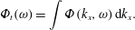 $$\begin{eqnarray}\unicode[STIX]{x1D6F7}_{t}(\unicode[STIX]{x1D714})=\int \unicode[STIX]{x1D6F7}(k_{x},\unicode[STIX]{x1D714})\,\text{d}k_{x}.\end{eqnarray}$$
The space–time energy spectra can be alternatively expressed using cross-correlations of temporal Fourier modes  $\hat{u} (x,\unicode[STIX]{x1D714})$ at two different locations
 $x$ and
 $x+r$:
 $$\begin{eqnarray}\frac{\unicode[STIX]{x1D6F7}(k_{x},\unicode[STIX]{x1D714})}{\unicode[STIX]{x1D6F7}_{t}(\unicode[STIX]{x1D714})}=\frac{1}{2\unicode[STIX]{x03C0}}\int \frac{\langle \hat{u} ^{\ast }(x,\unicode[STIX]{x1D714})\hat{u} (x+r,\unicode[STIX]{x1D714})\rangle }{\langle \hat{u} ^{\ast }(x,\unicode[STIX]{x1D714})\hat{u} (x,\unicode[STIX]{x1D714})\rangle }\text{e}^{-\text{i}k_{x}r}\,\text{d}r.\end{eqnarray}$$
If the temporal Fourier mode  $\hat{u} (x,\unicode[STIX]{x1D714})$ is expressed in terms of its amplitude
 $a(x,\unicode[STIX]{x1D714})$ and phase
 $\unicode[STIX]{x1D703}(x,\unicode[STIX]{x1D714})$, such as
 $$\begin{eqnarray}\hat{u} (x,\unicode[STIX]{x1D714})=a(x,\unicode[STIX]{x1D714})\text{e}^{\text{i}\unicode[STIX]{x1D703}(x,\unicode[STIX]{x1D714})},\end{eqnarray}$$
we have
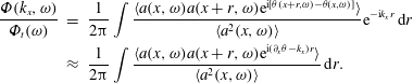 $$\begin{eqnarray}\displaystyle \frac{\unicode[STIX]{x1D6F7}(k_{x},\unicode[STIX]{x1D714})}{\unicode[STIX]{x1D6F7}_{t}(\unicode[STIX]{x1D714})} & = & \displaystyle \frac{1}{2\unicode[STIX]{x03C0}}\int \frac{\langle a(x,\unicode[STIX]{x1D714})a(x+r,\unicode[STIX]{x1D714})\text{e}^{\text{i}[\unicode[STIX]{x1D703}(x+r,\unicode[STIX]{x1D714})-\unicode[STIX]{x1D703}(x,\unicode[STIX]{x1D714})]}\rangle }{\langle a^{2}(x,\unicode[STIX]{x1D714})\rangle }\text{e}^{-\text{i}k_{x}r}\,\text{d}r\nonumber\\ \displaystyle & {\approx} & \displaystyle \frac{1}{2\unicode[STIX]{x03C0}}\int \frac{\langle a(x,\unicode[STIX]{x1D714})a(x+r,\unicode[STIX]{x1D714})\text{e}^{\text{i}(\unicode[STIX]{x2202}_{x}\unicode[STIX]{x1D703}-k_{x})r}\rangle }{\langle a^{2}(x,\unicode[STIX]{x1D714})\rangle }\,\text{d}r.\end{eqnarray}$$
In the above derivations, the Taylor series expansion of the phase  $\unicode[STIX]{x1D703}(x+r,\unicode[STIX]{x1D714})$ at location
 $x$ is taken up to the first order, and the exponential function
 $\text{e}^{-\text{i}k_{x}r}$ is moved into the angle brackets (ensemble average). A linear approximation of the phase difference is used in (2.6) for space–time energy spectra. The approximation is valid if the spatial separation
 $r$ has the order of the characteristic length scale at which the local wavenumber varies. This can be seen by the comparison of the second-order term with the first term in the Taylor expansion of the phase difference. The characteristic length scale thus obtained is given by
 $r\ll (1+U/\sqrt{\langle u^{2}\rangle })(k_{x}^{loc})^{-1}$, where
 $k_{x}^{loc}=\unicode[STIX]{x2202}_{x}\unicode[STIX]{x1D703}$ is the local wavenumber,
 $U$ is a local mean velocity and
 $u$ is a local velocity fluctuation.
We now introduce the LMW model and postpone its mathematical derivation to the later part of this subsection (see (2.15), (2.16) and (2.17)). The space–time energy spectra in (2.4) and (2.6) can be interpreted as ensemble averages of spatial and/or temporal Fourier modes. This suggests that, if the Fourier modes are represented by certain energetic flow structures, space–time energy spectra can thus be determined from the ensemble averages of the flow structures.
The simplest representation of a temporal Fourier mode is a travelling wave of propagation speed  $U$. In this case,
 $$\begin{eqnarray}\displaystyle & \displaystyle a(x+r,\unicode[STIX]{x1D714})=a(x,\unicode[STIX]{x1D714}), & \displaystyle\end{eqnarray}$$
 $$\begin{eqnarray}\displaystyle & \displaystyle \unicode[STIX]{x1D703}(x+r,\unicode[STIX]{x1D714})-\unicode[STIX]{x1D703}(x,\unicode[STIX]{x1D714})=\displaystyle \frac{\unicode[STIX]{x1D714}}{U}r. & \displaystyle\end{eqnarray}$$
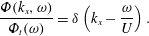 $$\begin{eqnarray}\frac{\unicode[STIX]{x1D6F7}(k_{x},\unicode[STIX]{x1D714})}{\unicode[STIX]{x1D6F7}_{t}(\unicode[STIX]{x1D714})}=\unicode[STIX]{x1D6FF}\left(k_{x}-\frac{\unicode[STIX]{x1D714}}{U}\right).\end{eqnarray}$$
This result is consistent with Taylor’s frozen-flow hypothesis but incorrectly predicts the spectral bandwidth to be zero.
Beall et al. (Reference Beall, Kim and Powers1982) introduced a local wave to represent the temporal Fourier modes, wherein the phase was approximated by a first-order Taylor series expansion, such that
 $$\begin{eqnarray}\displaystyle & \displaystyle a(x+r,\unicode[STIX]{x1D714})=a(x,\unicode[STIX]{x1D714}), & \displaystyle\end{eqnarray}$$
 $$\begin{eqnarray}\displaystyle & \displaystyle \unicode[STIX]{x1D703}(x+r,\unicode[STIX]{x1D714})=\unicode[STIX]{x1D703}(x,\unicode[STIX]{x1D714})+\unicode[STIX]{x2202}_{x}\unicode[STIX]{x1D703}\cdot r. & \displaystyle\end{eqnarray}$$
 $$\begin{eqnarray}\frac{\unicode[STIX]{x1D6F7}^{LW}(k_{x},\unicode[STIX]{x1D714})}{\unicode[STIX]{x1D6F7}_{t}(\unicode[STIX]{x1D714})}=\frac{\langle a^{2}(x,\unicode[STIX]{x1D714})\unicode[STIX]{x1D6FF}(k_{x}-\unicode[STIX]{x2202}_{x}\unicode[STIX]{x1D703})\rangle }{\langle a^{2}(x,\unicode[STIX]{x1D714})\rangle }.\end{eqnarray}$$
Here, and throughout this paper, the superscript ‘ $LW$’ denotes a result from the LW model. It will be seen in § 2.2 that this result exactly predicts the first-order moment and under-predicts the second-order moment.
To correctly predict the spectral bandwidths, we introduce local modulated waves to represent the temporal Fourier modes. In the present study, a local modulated wave is defined as a wave-like structure of a single frequency and two distinct wavenumbers. It is mathematically expressed by
 $$\begin{eqnarray}\displaystyle \hat{u} (x+r,\unicode[STIX]{x1D714}) & = & \displaystyle \hat{u} (x,\unicode[STIX]{x1D714})\left[\frac{\text{e}^{\text{i}(a^{-1}\unicode[STIX]{x2202}_{x}a\cdot r-\unicode[STIX]{x03C0}/4)}}{\sqrt{2}}+\frac{\text{e}^{-\text{i}(a^{-1}\unicode[STIX]{x2202}_{x}a\cdot r-\unicode[STIX]{x03C0}/4)}}{\sqrt{2}}\right]\text{e}^{\text{i}\unicode[STIX]{x2202}_{x}\unicode[STIX]{x1D703}\cdot r}\nonumber\\ \displaystyle & = & \displaystyle \hat{u} (x,\unicode[STIX]{x1D714})\cdot \sqrt{2}\cos (a^{-1}\unicode[STIX]{x2202}_{x}a\cdot r-\unicode[STIX]{x03C0}/4)\text{e}^{\text{i}\unicode[STIX]{x2202}_{x}\unicode[STIX]{x1D703}\cdot r}.\end{eqnarray}$$
In this case, the amplitude and phase of the local modulated wave downstream are related to those upstream by
 $$\begin{eqnarray}\displaystyle a(x+r,\unicode[STIX]{x1D714}) & = & \displaystyle a(x,\unicode[STIX]{x1D714})\left[\frac{\text{e}^{\text{i}(a^{-1}\unicode[STIX]{x2202}_{x}a\cdot r-\unicode[STIX]{x03C0}/4)}}{\sqrt{2}}+\frac{\text{e}^{-\text{i}(a^{-1}\unicode[STIX]{x2202}_{x}a\cdot r-\unicode[STIX]{x03C0}/4)}}{\sqrt{2}}\right]\nonumber\\ \displaystyle & {\approx} & \displaystyle a(x,\unicode[STIX]{x1D714})+\unicode[STIX]{x2202}_{x}a\cdot r,\end{eqnarray}$$
 $$\begin{eqnarray}\unicode[STIX]{x1D703}(x+r,\unicode[STIX]{x1D714})=\unicode[STIX]{x1D703}(x,\unicode[STIX]{x1D714})+\unicode[STIX]{x2202}_{x}\unicode[STIX]{x1D703}\cdot r.\end{eqnarray}$$
It can be found from (2.12a) and (2.12b) that (2.11) is exactly the same as the first-order Taylor expansions of both amplitude and phase. Therefore, (2.11) effectively represents a spatially localized wave-like structure due to the local validity of the Taylor expansion. Beall et al. (Reference Beall, Kim and Powers1982) utilized the first-order Taylor expansion of phase. The new development in this paper is that we utilize the first-order Taylor expansions of both amplitude and phase. Here,  $a^{-1}\unicode[STIX]{x2202}_{x}a$ represents the characteristic length scales of the amplitude variations. The phase delay
 $\unicode[STIX]{x03C0}/4$ and the factor
 $\sqrt{2}$ are used such that (2.11) is consistent with the first-order Taylor expansion. Meanwhile, they can also guarantee that the integral of the space–time energy spectrum with respect to the wavenumber is equal to its marginal distribution, i.e.
 $\int \unicode[STIX]{x1D6F7}(k_{x},\unicode[STIX]{x1D714})\,\text{d}k_{x}=\unicode[STIX]{x1D6F7}_{t}(\unicode[STIX]{x1D714})$ (temporal energy spectrum).
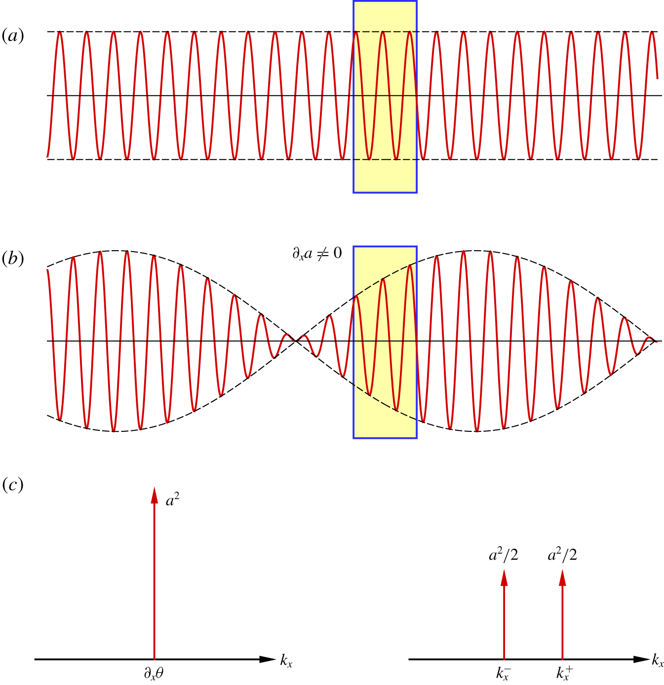
In fact, according to the first expression of (2.11), a local modulated wave can be thought of as the superposition of two waves. Meanwhile, the local modulated wave can also be thought of as the product of two waves in terms of the second expression of (2.11). The one associated with the phase derivative is the carrier wave, and the one associated with the amplitude derivative is the wave envelope. The wave envelope modulates the carrier wave, which appears as a local modulated wave. Figure 1 shows the sketches of the local wave and local modulated wave, where the former is the local wave structure of a single wavenumber and the latter is the local wave-like structure of two wavenumbers. Therefore, a local modulated wave is the wavepacket of two wavenumbers.
Upon substituting (2.11) into (2.6) and invoking the homogeneity assumption  $\langle \hat{u} ^{\ast }(x,\unicode[STIX]{x1D714})\hat{u} (x+r,\unicode[STIX]{x1D714})\rangle =\langle \hat{u} ^{\ast }(x-r,\unicode[STIX]{x1D714})\hat{u} (x,\unicode[STIX]{x1D714})\rangle$, we perform the Fourier transform on the resulting equation with respect to
 $r$. It is easily found that the imaginary parts of the space–time energy spectra
 $\unicode[STIX]{x1D6F7}(k_{x},\unicode[STIX]{x1D714})$ are zero. Therefore, we obtain the LMW model
 $$\begin{eqnarray}\frac{\unicode[STIX]{x1D6F7}^{LMW}(k_{x},\unicode[STIX]{x1D714})}{\unicode[STIX]{x1D6F7}_{t}(\unicode[STIX]{x1D714})}=\frac{\langle a^{2}(x,\unicode[STIX]{x1D714})\unicode[STIX]{x1D6FF}(k_{x}-k_{x}^{+}(x,\unicode[STIX]{x1D714}))\rangle }{2\langle a^{2}(x,\unicode[STIX]{x1D714})\rangle }+\frac{\langle a^{2}(x,\unicode[STIX]{x1D714})\unicode[STIX]{x1D6FF}(k_{x}-k_{x}^{-}(x,\unicode[STIX]{x1D714}))\rangle }{2\langle a^{2}(x,\unicode[STIX]{x1D714})\rangle },\end{eqnarray}$$
where
 $$\begin{eqnarray}\displaystyle & \displaystyle k_{x}^{+}(x,\unicode[STIX]{x1D714})=\unicode[STIX]{x2202}_{x}\unicode[STIX]{x1D703}+a^{-1}\unicode[STIX]{x2202}_{x}a, & \displaystyle\end{eqnarray}$$
 $$\begin{eqnarray}\displaystyle & \displaystyle k_{x}^{-}(x,\unicode[STIX]{x1D714})=\unicode[STIX]{x2202}_{x}\unicode[STIX]{x1D703}-a^{-1}\unicode[STIX]{x2202}_{x}a. & \displaystyle\end{eqnarray}$$
 $LMW$’ denotes the results from the LMW model. The form of (2.13) is similar to that of the grained probability density functions (Pope Reference Pope2000). If the velocity fluctuation
 $u(x,t)$ is statistically homogeneous in space, the ensemble average can be taken as the spatial average over all locations
 $x$. As a result, (2.13) implies that the space–time energy spectra at wavenumber
 $k_{x}$ are the spatial average of the squared amplitudes over the locations
 $x$ at which the wavenumber
 $k_{x}^{+}$ or
 $k_{x}^{-}$ is equal to the wavenumber
 $k_{x}$. In other words, the present model proposes that if a velocity field is approximately represented by local modulated waves of wavenumber
 $k_{x}^{+}$ and
 $k_{x}^{-}$, the energy density at each wavenumber
 $k_{x}$ is the average of the energy densities of these carrier waves and wave envelopes with the same wavenumber
 $k_{x}$, i.e.
 $k_{x}^{+}=k_{x}$ and
 $k_{x}^{-}=k_{x}$. Therefore, (2.13) implies that space–time energy spectra are the ensemble averages of energetic wave-like structures of the wavenumber
 $k_{x}$ at given frequency
 $\unicode[STIX]{x1D714}$. It will be seen in § 2.2 that (2.13) can exactly predict the first- and second-order moments of space–time energy spectra.
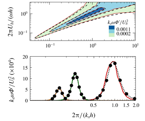
Schematic of (a) a local wave and (b) a local modulated wave in yellow shades; (c) energy spectra of local waves and local modulated waves.

We will show that the space–time energy spectra take the form of (2.13) under the following three conditions: (i) the amplitudes are approximated by a second-order Taylor expansion; (ii) the phase is approximated by a first-order Taylor expansion; and (iii) the amplitude and phase are weakly correlated. These conditions are less stringent than those of the LW model (Beall et al. Reference Beall, Kim and Powers1982). The cross-correlation of the amplitudes  $a(x,\unicode[STIX]{x1D714})$ and
 $a(x+r,\unicode[STIX]{x1D714})$ can be estimated using a Taylor series expansion up to the second order and the homogeneity assumption
 $$\begin{eqnarray}\displaystyle \langle a(x,\unicode[STIX]{x1D714})a(x+r,\unicode[STIX]{x1D714})\rangle & {\approx} & \displaystyle \langle a^{2}\rangle +\langle a\unicode[STIX]{x2202}_{x}a\rangle r+{\textstyle \frac{1}{2}}\langle a\unicode[STIX]{x2202}_{xx}^{2}a\rangle r^{2}\nonumber\\ \displaystyle & = & \displaystyle \langle a^{2}\rangle -{\textstyle \frac{1}{2}}\langle (\unicode[STIX]{x2202}_{x}a)^{2}\rangle r^{2}.\end{eqnarray}$$
It is also noted that the following identity holds
 $$\begin{eqnarray}{\textstyle \frac{1}{2}}a^{2}[\text{e}^{\text{i}a^{-1}\unicode[STIX]{x2202}_{x}a\cdot r}+\text{e}^{-\text{i}a^{-1}\unicode[STIX]{x2202}_{x}a\cdot r}]=a^{2}\cos (a^{-1}\unicode[STIX]{x2202}_{x}a\cdot r)\approx a^{2}-{\textstyle \frac{1}{2}}(\unicode[STIX]{x2202}_{x}a)^{2}r^{2}.\end{eqnarray}$$
A comparison of (2.16) with (2.15) yields
 $$\begin{eqnarray}\langle a(x,\unicode[STIX]{x1D714})a(x+r,\unicode[STIX]{x1D714})\rangle \approx {\textstyle \frac{1}{2}}\langle a^{2}[\text{e}^{\text{i}a^{-1}\unicode[STIX]{x2202}_{x}a\cdot r}+\text{e}^{-\text{i}a^{-1}\unicode[STIX]{x2202}_{x}a\cdot r}]\rangle .\end{eqnarray}$$
Substituting (2.17) into (2.6) with the weakly correlated assumption of the amplitude and phase leads to (2.13).
The present model implies that if a velocity field is approximately represented by local modulated waves of wavenumbers  $k_{x}^{+}$ and
 $k_{x}^{-}$, then the energy density at wavenumber
 $k_{x}$ is the ensemble average of the energy density of these waves and their envelopes with the same wavenumber
 $k_{x}$, i.e.
 $k_{x}^{+}=k_{x}$ and
 $k_{x}^{-}=k_{x}$.
This model can be used to reconstruct space–time energy spectra from the time series of velocity components at an array of in-line spatial locations. We will show in § 2.2 that the present model can exactly predict the first- and second-order moments of energy spectra. If temporal information is obtained from experimental or numerical measurements, we can calculate the temporal Fourier modes and reconstruct the space–time energy spectra.
The decomposition of the local modulated waves into two waves with the same frequency but different wavenumbers can also be performed for the same wavenumber with two distinct frequencies. The former is suitable for the time series of velocity fluctuations at two or a limited number of measurement points, which is conveniently transformed into temporal Fourier modes, and the latter is suitable for the spatial series of velocity fluctuations with a short-term record, which is readily transformed into spatial Fourier modes. In experimental measurements such as HWA and LDA, the long-term records at a few measurement points are far more likely to be obtained than the spatial series of long lengths with short-term records. Therefore, the present study focuses on the local modulated waves of one frequency and two different wavenumbers.
The present model is consistent with the dominating processes of temporal decorrelation in turbulent flows. Temporal decorrelation is dominated by the following three processes: the convection of small-scale structures by large-scale structures, the interaction between small-scale structures and the stretching of small-scale structures by large-scale structures. The first process is primarily characterized by Taylor’s frozen-flow hypothesis (Taylor Reference Taylor1938), and the second process is determined by the Kraichnan–Tennekes random sweeping hypothesis (Kraichnan Reference Kraichnan1964; Tennekes Reference Tennekes1975). The present work proposes that the third process can be approximately modelled by local modulated waves. If small-scale structures are approximated as local waves, large-scale stretching modifies the amplitudes of small-scale structures and consequently generates local modulated waves. This is particularly evident for slow-evolving large-scale flow structures and rapid-distorting small-scale flow structures.
The present work proposes that space–time energy spectra can be reconstructed from statistical averages of energetic flow structures. In the LW model, a local wave of a single wavenumber is introduced to represent an energetic flow structure. The obtained result correctly predicts the first-order moments of the space–time energy spectra but under-predicts the second-order moments. In the present LMW model, a local modulated wave of two local wavenumbers is introduced to represent the energetic flow structure. The obtained result correctly predicts the first- and second-order moments of the space–time energy spectra. Consequently, a high-order approximation can be achieved if a wavepacket of more local wavenumbers is introduced to represent the energetic flow structure. This constitutes a structure-based statistical approximation.
2.2 Mean wavenumbers and spectral bandwidths
A space–time energy spectrum  $\unicode[STIX]{x1D6F7}(k_{x},\unicode[STIX]{x1D714})$ is a two-dimensional distribution of the energy density with respect to the wavenumber and frequency. Analogously to the case of a joint probability density function, a conditional distribution
 $\unicode[STIX]{x1D6F7}(k_{x}|\unicode[STIX]{x1D714}_{0})$ can be introduced to describe the wavenumber spectrum of the energy density at a given frequency
 $\unicode[STIX]{x1D714}_{0}$, such that
 $\unicode[STIX]{x1D6F7}(k_{x}|\unicode[STIX]{x1D714}_{0})=\unicode[STIX]{x1D6F7}(k_{x},\unicode[STIX]{x1D714}_{0})/\unicode[STIX]{x1D6F7}_{t}(\unicode[STIX]{x1D714}_{0})$. Conditional distributions are cuts through space–time energy spectra at a given frequency. Furthermore, we introduce the first- and second-order conditional moments as
 $$\begin{eqnarray}k_{xc}(\unicode[STIX]{x1D714}_{0})=\int k_{x}\unicode[STIX]{x1D6F7}(k_{x}|\unicode[STIX]{x1D714}_{0})\,\text{d}k_{x}\end{eqnarray}$$
and
 $$\begin{eqnarray}B(\unicode[STIX]{x1D714}_{0})=\int [k_{x}-k_{xc}(\unicode[STIX]{x1D714}_{0})]^{2}\unicode[STIX]{x1D6F7}(k_{x}|\unicode[STIX]{x1D714}_{0})\,\text{d}k_{x},\end{eqnarray}$$
which represent the mean wavenumbers and standard deviations of the conditional distributions, respectively.
The first-order conditional moments indicate the mean wavenumbers, which represent the mass centres of the conditional distributions of the energy densities. The mean wavenumbers are often used to estimate the frequency-dependent convection velocity, such that  $U_{c}(\unicode[STIX]{x1D714})=\unicode[STIX]{x1D714}/k_{xc}(\unicode[STIX]{x1D714})$ (Renard & Deck Reference Renard and Deck2015). The second-order conditional moments indicate the bandwidths of the energy spectra. The spectral bandwidths are used to study the well-known ‘spectral broadening’ in turbulent flows (Lumley Reference Lumley1965; Wilczek & Narita Reference Wilczek and Narita2012; Wilczek et al. Reference Wilczek, Stevens and Meneveau2015; Wu et al. Reference Wu, Geng, Yao, Xu and He2017).
The mean wavenumber and spectral bandwidth can be exactly expressed using temporal Fourier modes, given by (Wu et al. Reference Wu, Geng, Yao, Xu and He2017)
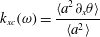 $$\begin{eqnarray}k_{xc}(\unicode[STIX]{x1D714})=\frac{\langle a^{2}\unicode[STIX]{x2202}_{x}\unicode[STIX]{x1D703}\rangle }{\langle a^{2}\rangle }\end{eqnarray}$$
and
 $$\begin{eqnarray}B(\unicode[STIX]{x1D714})=\frac{\langle a^{2}(\unicode[STIX]{x2202}_{x}\unicode[STIX]{x1D703}-k_{xc})^{2}\rangle }{\langle a^{2}\rangle }+\frac{\langle (\unicode[STIX]{x2202}_{x}a)^{2}\rangle }{\langle a^{2}\rangle }.\end{eqnarray}$$
The mean wavenumbers are determined by phase derivatives alone, and the spectral bandwidths are determined by changes in both phase and amplitude. Our numerical simulations (Wu et al. Reference Wu, Geng, Yao, Xu and He2017) show that the contribution of amplitude derivatives to the spectral bandwidth is not small compared to the phase contribution at a Reynolds number of  $Re_{\unicode[STIX]{x1D70F}}=550$ in turbulent channel flows. Therefore, the contribution of amplitude derivatives to spectral bandwidths cannot be ignored.
We now show that the LMW model exactly predicts the mean wavenumbers and spectral bandwidths. For this purpose, we substitute the LMW model (2.13) into (2.18) for the mean wavenumbers, which yields
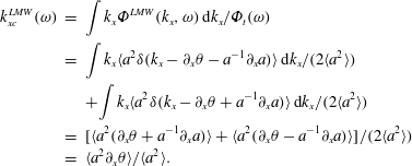 $$\begin{eqnarray}\displaystyle k_{xc}^{\,LMW}(\unicode[STIX]{x1D714}) & = & \displaystyle \int k_{x}\unicode[STIX]{x1D6F7}^{LMW}(k_{x},\unicode[STIX]{x1D714})\,\text{d}k_{x}/\unicode[STIX]{x1D6F7}_{t}(\unicode[STIX]{x1D714})\nonumber\\ \displaystyle & = & \displaystyle \int k_{x}\langle a^{2}\unicode[STIX]{x1D6FF}(k_{x}-\unicode[STIX]{x2202}_{x}\unicode[STIX]{x1D703}-a^{-1}\unicode[STIX]{x2202}_{x}a)\rangle \,\text{d}k_{x}/(2\langle a^{2}\rangle )\nonumber\\ \displaystyle & & \displaystyle +\int k_{x}\langle a^{2}\unicode[STIX]{x1D6FF}(k_{x}-\unicode[STIX]{x2202}_{x}\unicode[STIX]{x1D703}+a^{-1}\unicode[STIX]{x2202}_{x}a)\rangle \,\text{d}k_{x}/(2\langle a^{2}\rangle )\nonumber\\ \displaystyle & = & \displaystyle [\langle a^{2}(\unicode[STIX]{x2202}_{x}\unicode[STIX]{x1D703}+a^{-1}\unicode[STIX]{x2202}_{x}a)\rangle +\langle a^{2}(\unicode[STIX]{x2202}_{x}\unicode[STIX]{x1D703}-a^{-1}\unicode[STIX]{x2202}_{x}a)\rangle ]/(2\langle a^{2}\rangle )\nonumber\\ \displaystyle & = & \displaystyle \langle a^{2}\unicode[STIX]{x2202}_{x}\unicode[STIX]{x1D703}\rangle /\langle a^{2}\rangle .\end{eqnarray}$$
Therefore, upon comparing the above expression with (2.20), we have  $k_{xc}^{\,LMW}(\unicode[STIX]{x1D714})=k_{xc}(\unicode[STIX]{x1D714})$. Similarly, we can show that
 $k_{xc}^{LW}(\unicode[STIX]{x1D714})=\langle a^{2}\unicode[STIX]{x2202}_{x}\unicode[STIX]{x1D703}\rangle /\langle a^{2}\rangle$. Next, we substitute the LMW model (2.13) into (2.19) for spectral bandwidths to obtain
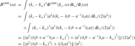 $$\begin{eqnarray}\displaystyle B^{LMW}(\unicode[STIX]{x1D714}) & = & \displaystyle \int (k_{x}-k_{xc})^{2}\unicode[STIX]{x1D6F7}^{LMW}(k_{x},\unicode[STIX]{x1D714})\,\text{d}k_{x}/\unicode[STIX]{x1D6F7}_{t}(\unicode[STIX]{x1D714})\nonumber\\ \displaystyle & = & \displaystyle \int (k_{x}-k_{xc})^{2}\langle a^{2}\unicode[STIX]{x1D6FF}(k_{x}-\unicode[STIX]{x2202}_{x}\unicode[STIX]{x1D703}-a^{-1}\unicode[STIX]{x2202}_{x}a)\rangle \,\text{d}k_{x}/(2\langle a^{2}\rangle )\nonumber\\ \displaystyle & & \displaystyle +\int (k_{x}-k_{xc})^{2}\langle a^{2}\unicode[STIX]{x1D6FF}(k_{x}-\unicode[STIX]{x2202}_{x}\unicode[STIX]{x1D703}+a^{-1}\unicode[STIX]{x2202}_{x}a)\rangle \,\text{d}k_{x}/(2\langle a^{2}\rangle )\nonumber\\ \displaystyle & = & \displaystyle [\langle a^{2}(\unicode[STIX]{x2202}_{x}\unicode[STIX]{x1D703}+a^{-1}\unicode[STIX]{x2202}_{x}a-k_{xc})^{2}\rangle +\langle a^{2}(\unicode[STIX]{x2202}_{x}\unicode[STIX]{x1D703}-a^{-1}\unicode[STIX]{x2202}_{x}a-k_{xc})^{2}\rangle ]/(2\langle a^{2}\rangle )\nonumber\\ \displaystyle & = & \displaystyle [\langle a^{2}(\unicode[STIX]{x2202}_{x}\unicode[STIX]{x1D703}-k_{xc})^{2}\rangle +\langle (\unicode[STIX]{x2202}_{x}a)^{2}\rangle ]/\langle a^{2}\rangle .\end{eqnarray}$$
Accordingly, upon comparing the above expression with (2.21), we have  $B^{LMW}(\unicode[STIX]{x1D714})=B(\unicode[STIX]{x1D714})$. Similarly, we can show that
 $B^{LW}(\unicode[STIX]{x1D714})=\langle a^{2}(\unicode[STIX]{x2202}_{x}\unicode[STIX]{x1D703}-k_{xc})^{2}\rangle /\langle a^{2}\rangle$.
The exact expression (2.20) implies that the first-order conditional moments are fully determined by the energy-weighted averages of the phase derivatives. It is noted that the LW model and LMW model include the contributions of phase derivatives. As a result, these two models can correctly predict the first-order conditional moments. The exact expression (2.21) indicates that the spectral bandwidths are determined by both phase and amplitude derivatives. However, the LW model excludes the contribution of amplitude derivatives and thus under-predicts the spectral bandwidths. The LMW model can correctly predict the spectral bandwidths since it takes into account the contributions of both phase and amplitude derivatives.
2.3 Numerical procedure
This section presents a numerical procedure to reconstruct space–time energy spectra. The numerical procedure is based on the LMW model and will be illustrated and validated in §§ 3 and 4, respectively. The input for the numerical procedure is a non-periodic and incomplete dataset of velocity fluctuations  $u(x_{i},t_{j})$ at spatial points
 $x_{i}$ and discrete times
 $t_{j}$. Although the procedure is presented for a one-dimensional random field, it can be extended to turbulent channel flows.
The numerical procedure for the LMW model is described as follows:
(i) We perform Fourier transforms to obtain the temporal Fourier modes of the velocity fluctuations  $u(x,t)$:
 $$\begin{eqnarray}\hat{u} (x,\unicode[STIX]{x1D714})=\frac{1}{\sqrt{T\int _{0}^{T}w(t)^{2}\,\text{d}t}}\int _{0}^{T}w(t)u(x,t)\text{e}^{\text{i}\unicode[STIX]{x1D714}t}\,\text{d}t,\end{eqnarray}$$
wherein a Hanning window  $w(t)$ is used and the window length
 $T$ is taken as the maximal time scale.
(ii) We calculate the cross-spectra  $\unicode[STIX]{x1D6F9}(x,\unicode[STIX]{x0394}x,\unicode[STIX]{x1D714})$ of the temporal Fourier modes at two different spatial locations
 $x$ and
 $x+\unicode[STIX]{x0394}x$:
 $$\begin{eqnarray}\unicode[STIX]{x1D6F9}(x,\unicode[STIX]{x0394}x,\unicode[STIX]{x1D714})\equiv \hat{u} ^{\ast }(x,\unicode[STIX]{x1D714})\hat{u} (x+\unicode[STIX]{x0394}x,\unicode[STIX]{x1D714}).\end{eqnarray}$$
Consequently, we find the cross-spectral energy  $|\unicode[STIX]{x1D6F9}|$ and the phase difference
 $\unicode[STIX]{x0394}\unicode[STIX]{x1D703}\equiv \arg (\unicode[STIX]{x1D6F9})=\unicode[STIX]{x1D703}(x+\unicode[STIX]{x0394}x,\unicode[STIX]{x1D714})-\unicode[STIX]{x1D703}(x,\unicode[STIX]{x1D714})$. Here,
 $\text{arg}$ is denoted as the phase of a complex variable;
 $\unicode[STIX]{x0394}\unicode[STIX]{x1D703}$ is calculated by the unfolding technique (Buxton, de Kat & Ganapathisubramani Reference Buxton, de Kat and Ganapathisubramani2013; de Kat & Ganapathisubramani Reference de Kat and Ganapathisubramani2015), such that
 $\unicode[STIX]{x0394}\unicode[STIX]{x1D703}$ is located in the range of
 $\unicode[STIX]{x1D714}\unicode[STIX]{x0394}x/U_{c}-\unicode[STIX]{x03C0}<\unicode[STIX]{x0394}\unicode[STIX]{x1D703}<\unicode[STIX]{x1D714}\unicode[STIX]{x0394}x/U_{c}+\unicode[STIX]{x03C0}$ with
 $U_{c}$ being the convection velocity.
(iii) The amplitude and phase derivatives of the temporal Fourier modes are calculated using the finite-difference approximation
 $$\begin{eqnarray}\displaystyle & \displaystyle \unicode[STIX]{x2202}_{x}\unicode[STIX]{x1D703}=\displaystyle \frac{\unicode[STIX]{x0394}\unicode[STIX]{x1D703}}{\unicode[STIX]{x0394}x}, & \displaystyle\end{eqnarray}$$
 $$\begin{eqnarray}\displaystyle & \displaystyle \unicode[STIX]{x2202}_{x}a=\displaystyle \frac{\unicode[STIX]{x0394}a}{\unicode[STIX]{x0394}x}\equiv \frac{a(x+\unicode[STIX]{x0394}x,\unicode[STIX]{x1D714})-a(x,\unicode[STIX]{x1D714})}{\unicode[STIX]{x0394}x}. & \displaystyle\end{eqnarray}$$
(iv) Two distinct wavenumbers of a local modulated wave are determined from their definitions (2.14), such that
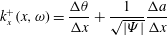 $$\begin{eqnarray}k_{x}^{+}(x,\unicode[STIX]{x1D714})=\frac{\unicode[STIX]{x0394}\unicode[STIX]{x1D703}}{\unicode[STIX]{x0394}x}+\frac{1}{\sqrt{|\unicode[STIX]{x1D6F9}|}}\frac{\unicode[STIX]{x0394}a}{\unicode[STIX]{x0394}x}\end{eqnarray}$$
and
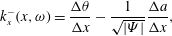 $$\begin{eqnarray}k_{x}^{-}(x,\unicode[STIX]{x1D714})=\frac{\unicode[STIX]{x0394}\unicode[STIX]{x1D703}}{\unicode[STIX]{x0394}x}-\frac{1}{\sqrt{|\unicode[STIX]{x1D6F9}|}}\frac{\unicode[STIX]{x0394}a}{\unicode[STIX]{x0394}x},\end{eqnarray}$$
where the amplitude  $a$ is estimated by the square root of the cross-spectral energy
 $\sqrt{|\unicode[STIX]{x1D6F9}|}$.
(v) The energy spectra corresponding to wavenumbers  $k_{x}^{+}$ and
 $k_{x}^{-}$ of the local modulated waves are estimated from the cross-spectra
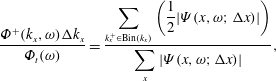 $$\begin{eqnarray}\displaystyle & \displaystyle \frac{\unicode[STIX]{x1D6F7}^{+}(k_{x},\unicode[STIX]{x1D714})\unicode[STIX]{x0394}k_{x}}{\unicode[STIX]{x1D6F7}_{t}(\unicode[STIX]{x1D714})}=\frac{\displaystyle \mathop{\sum }_{k_{x}^{+}\in \text{Bin}(k_{x})}\left(\frac{1}{2}|\unicode[STIX]{x1D6F9}(x,\unicode[STIX]{x1D714};\unicode[STIX]{x0394}x)|\right)}{\displaystyle \mathop{\sum }_{x}|\unicode[STIX]{x1D6F9}(x,\unicode[STIX]{x1D714};\unicode[STIX]{x0394}x)|}, & \displaystyle\end{eqnarray}$$
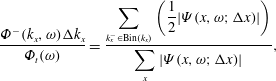 $$\begin{eqnarray}\displaystyle & \displaystyle \frac{\unicode[STIX]{x1D6F7}^{-}(k_{x},\unicode[STIX]{x1D714})\unicode[STIX]{x0394}k_{x}}{\unicode[STIX]{x1D6F7}_{t}(\unicode[STIX]{x1D714})}=\frac{\displaystyle \mathop{\sum }_{k_{x}^{-}\in \text{Bin}(k_{x})}\left(\frac{1}{2}|\unicode[STIX]{x1D6F9}(x,\unicode[STIX]{x1D714};\unicode[STIX]{x0394}x)|\right)}{\displaystyle \mathop{\sum }_{x}|\unicode[STIX]{x1D6F9}(x,\unicode[STIX]{x1D714};\unicode[STIX]{x0394}x)|}, & \displaystyle\end{eqnarray}$$
where the interval  $\text{Bin}(k_{x})\equiv [k_{x}-\unicode[STIX]{x0394}k_{x}/2,k_{x}+\unicode[STIX]{x0394}k_{x}/2]$ is centred at wavenumber
 $k_{x}$ with a small wavenumber bandwidth
 $\unicode[STIX]{x0394}k_{x}$. The summation in the numerator of (2.30) is taken for all locations
 $x$ such that the local wavenumbers
 $k_{x}^{+}(x,\unicode[STIX]{x1D714})$ belong to
 $\text{Bin}(k_{x})$. Similarly, the summation in the numerator of (2.31) is taken for all locations
 $x$ such that the wavenumbers
 $k_{x}^{-}(x,\unicode[STIX]{x1D714})$ belong to
 $\text{Bin}(k_{x})$. The summations in the denominators of (2.30) and (2.31) are taken for all locations
 $x$. The cross-spectral energy
 $|\unicode[STIX]{x1D6F9}|$ in (2.28), (2.29), (2.30) and (2.31) can be replaced by the averaged energy at the two points,
 $[a^{2}(x,\unicode[STIX]{x1D714})+a^{2}(x+\unicode[STIX]{x0394}x,\unicode[STIX]{x1D714})]/2$, which can conserve the energy of the space–time spectra as the averaged energies at the two points. Our numerical comparisons show that the results obtained from cross-spectral energy are very close to those from the averaged energy at the two points.
(vi) We finally calculate the sum of the energy spectra  $\unicode[STIX]{x1D6F7}^{+}$ and
 $\unicode[STIX]{x1D6F7}^{-}$ corresponding to
 $k_{x}^{+}$ and
 $k_{x}^{-}$, respectively, for the space–time energy spectra
 $$\begin{eqnarray}\unicode[STIX]{x1D6F7}^{LMW}(k_{x},\unicode[STIX]{x1D714})=\unicode[STIX]{x1D6F7}^{+}(k_{x},\unicode[STIX]{x1D714})+\unicode[STIX]{x1D6F7}^{-}(k_{x},\unicode[STIX]{x1D714}).\end{eqnarray}$$
The numerical procedure for one-dimensional random fields can be easily extended to calculate the space–time energy spectra of a single wavenumber and frequency for three-dimensional random fields, such as the joint streamwise-wavenumber and frequency energy spectra of streamwise components of three-dimensional velocity fields in turbulent channel flows. The corresponding changes for the numerical procedure are listed as follows: (i)  $u(x,t)$ and
 $\hat{u} (x,\unicode[STIX]{x1D714})$ in (2.24) and (2.25) are replaced separately by
 $u(x,t;y,z)$ and
 $\hat{u} (x,\unicode[STIX]{x1D714};y,z)\equiv a(x,\unicode[STIX]{x1D714};y,z)\exp [\text{i}\unicode[STIX]{x1D703}(x,\unicode[STIX]{x1D714};y,z)]$. Here,
 $u$ is a velocity component in the streamwise direction;
 $x$,
 $y$ and
 $z$ denote the coordinates in the streamwise, wall-normal and spanwise directions, respectively. For turbulent channel flows, the space–time energy spectra are dependent on the wall-normal height
 $y$. Therefore,
 $k_{x}^{\pm }(x,\unicode[STIX]{x1D714})$,
 $\unicode[STIX]{x1D6F7}^{\pm }(k_{x},\unicode[STIX]{x1D714})$,
 $\unicode[STIX]{x1D6F7}_{t}(\unicode[STIX]{x1D714})$ and
 $\unicode[STIX]{x1D6F7}^{LMW}(k_{x},\unicode[STIX]{x1D714})$ in (2.28)–(2.32) are replaced by
 $k_{x}^{\pm }(x,\unicode[STIX]{x1D714};y,z)$,
 $\unicode[STIX]{x1D6F7}^{\pm }(k_{x},\unicode[STIX]{x1D714};y)$,
 $\unicode[STIX]{x1D6F7}_{t}(\unicode[STIX]{x1D714};y)$ and
 $\unicode[STIX]{x1D6F7}^{LMW}(k_{x},\unicode[STIX]{x1D714};y)$, respectively. (ii) The summations in both the numerators and denominators of (2.30) and (2.31) should be carried out for all locations
 $z$ and for all locations
 $x$ at which certain wavenumbers are taken, since the streamwise velocity component is homogeneous in the spanwise direction
 $z$.
The LMW model can be used to correctly predict the mean wavenumbers and spectral bandwidths if (i) the measurement resolution  $\unicode[STIX]{x0394}x$ in space is reasonably small to correctly estimate the derivatives of phase and amplitude and (ii) the length of the measurement in time is sufficiently large to provide the ensemble of space–time signals to estimate the space–time energy spectra. In other words, the length of the time record is sufficiently large to allow the wave-like structures of wavelength
 $\unicode[STIX]{x1D706}$ to pass the entire measurement domain (of length
 $L_{x}$ in one-dimension) several times. Usually, the spatial resolution
 $\unicode[STIX]{x0394}x$ is smaller than the domain size (
 $\unicode[STIX]{x0394}x<L_{x}$) and required to be smaller than the wavelength (
 $\unicode[STIX]{x0394}x<\unicode[STIX]{x1D706}$). Therefore, if
 $\unicode[STIX]{x1D706}>L_{x}$, then
 $\unicode[STIX]{x0394}x<L_{x}<\unicode[STIX]{x1D706}$, which implies that the LMW model can be used for the wave-like structures of long wavelength that is comparable with the length scales of the measurement domains. However, at this moment, we do not intend to use the LMW model for reconstructing the instantaneous velocity fields, such as superstructures in the logarithmic and lower wake regions of turbulent boundary layers (Hutchins & Marusic Reference Hutchins and Marusic2007; Kevin, Monty & Hutchins Reference Kevin, Monty and Hutchins2019), which is a very interesting topic for future study.
3 An illustrative example for the LMW model
In this section, we use a simple example to illustrate and validate the LMW model. This example is a propagating Gaussian signal modulated by a non-propagating Gaussian amplitude, which takes the form of
 $$\begin{eqnarray}u(x,t)=\frac{1}{\sqrt{2\unicode[STIX]{x03C0}\unicode[STIX]{x1D70E}_{x}^{2}}}\frac{1}{\sqrt{2\unicode[STIX]{x03C0}\unicode[STIX]{x1D70E}_{t}^{2}}}\text{exp}\left(-\frac{x^{2}}{2\unicode[STIX]{x1D70E}_{x}^{2}}\right)\text{exp}\left\{-\frac{[t-x/(U+v)]^{2}}{2\unicode[STIX]{x1D70E}_{t}^{2}}\right\}.\end{eqnarray}$$
Here,  $\unicode[STIX]{x1D70E}_{x}$ is the spatial standard deviation of the non-propagating Gaussian amplitude and
 $\unicode[STIX]{x1D70E}_{t}$ is the temporal standard deviation of the propagating Gaussian signal;
 $U$ is a constant propagation speed;
 $v$ is a random sweeping velocity that satisfies a Gaussian distribution of zero mean and variance
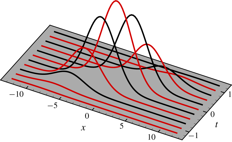
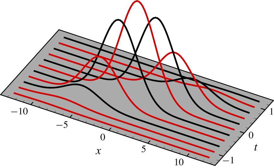
 $V^{2}$ and is independent of space and time. Figure 2 shows the temporal evolution of the function
 $u(x,t)$ for
 $\unicode[STIX]{x1D70E}_{x}=3.54$,
 $\unicode[STIX]{x1D70E}_{t}=0.24$,
 $U=12$ and
 $v=0$, from which we find that its amplitude and phase depend on both space and time.
The temporal evolution of  $u(x,t)$, a propagating Gaussian signal modulated by a non-propagating Gaussian amplitude, which is determined by (3.1). For the sake of clarity, the waveforms at adjacent moments are drawn as red and black lines, respectively.
To simplify the presentation, we now consider the case of  $v=0$. The results for
 $v\neq 0$ will be provided at the end of this section, with random phase effects included. In the case of
 $v=0$, the space–time energy spectrum of
 $u(x,t)$ is given by
 $$\begin{eqnarray}\unicode[STIX]{x1D6F7}(k_{x},\unicode[STIX]{x1D714})=\frac{\unicode[STIX]{x1D70E}_{x}}{\sqrt{\unicode[STIX]{x03C0}}}\text{exp}\left[-\unicode[STIX]{x1D70E}_{x}^{2}\left(k_{x}-\frac{\unicode[STIX]{x1D714}}{U}\right)^{2}\right]\unicode[STIX]{x1D6F7}_{t}(\unicode[STIX]{x1D714}).\end{eqnarray}$$
We substitute (3.2) into (2.18) and (2.19) to find the mean wavenumbers and spectral bandwidths, respectively,
 $$\begin{eqnarray}\displaystyle & \displaystyle k_{xc}(\unicode[STIX]{x1D714})=\int k_{x}\unicode[STIX]{x1D6F7}(k_{x}|\unicode[STIX]{x1D714})\,\text{d}k_{x}=\frac{\unicode[STIX]{x1D714}}{U}, & \displaystyle\end{eqnarray}$$
 $$\begin{eqnarray}\displaystyle & \displaystyle B(\unicode[STIX]{x1D714})=\int (k_{x}-k_{xc})^{2}\unicode[STIX]{x1D6F7}(k_{x}|\unicode[STIX]{x1D714})\,\text{d}k_{x}=\frac{1}{2\unicode[STIX]{x1D70E}_{x}^{2}}. & \displaystyle\end{eqnarray}$$
For the following discussion, we also calculate the temporal Fourier modes
 $$\begin{eqnarray}\hat{u} (x,\unicode[STIX]{x1D714})=a(0,\unicode[STIX]{x1D714})\text{exp}\left(-\frac{x^{2}}{2\unicode[STIX]{x1D70E}_{x}^{2}}\right)\text{exp}\left(\text{i}\frac{\unicode[STIX]{x1D714}x}{U}\right),\end{eqnarray}$$
and their amplitudes and phases
 $$\begin{eqnarray}\displaystyle & \displaystyle a(x,\unicode[STIX]{x1D714})=a(0,\unicode[STIX]{x1D714})\text{exp}\left(-\frac{x^{2}}{2\unicode[STIX]{x1D70E}_{x}^{2}}\right), & \displaystyle\end{eqnarray}$$
 $$\begin{eqnarray}\displaystyle & \displaystyle \unicode[STIX]{x1D703}(x,\unicode[STIX]{x1D714})=\frac{\unicode[STIX]{x1D714}x}{U}. & \displaystyle\end{eqnarray}$$
Taylor’s frozen-flow hypothesis cannot be applied to the present example, since  $u(x,t+\unicode[STIX]{x1D70F})\neq u(x-U\unicode[STIX]{x1D70F},t)$. The LW model also cannot be applied to the present example, since the amplitude derivative
 $\unicode[STIX]{x2202}_{x}a\neq 0$ explicitly depends on the location
 $x$. In fact, the local wavenumbers in this model are given by
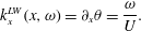 $$\begin{eqnarray}k_{x}^{LW}(x,\unicode[STIX]{x1D714})=\unicode[STIX]{x2202}_{x}\unicode[STIX]{x1D703}=\frac{\unicode[STIX]{x1D714}}{U}.\end{eqnarray}$$
Substitution of (3.8) into the LW model, equation (2.10), yields the space–time energy spectrum
 $$\begin{eqnarray}\unicode[STIX]{x1D6F7}^{LW}(k_{x},\unicode[STIX]{x1D714})=\unicode[STIX]{x1D6F7}_{t}(\unicode[STIX]{x1D714})\unicode[STIX]{x1D6FF}(k_{x}-\unicode[STIX]{x1D714}/U).\end{eqnarray}$$
According to (3.9), we find the mean wavenumber  $k_{xc}^{LW}(\unicode[STIX]{x1D714})=\unicode[STIX]{x1D714}/U$ and the spectral bandwidth
 $B^{LW}(\unicode[STIX]{x1D714})=0$. The latter is different from the exact result, as given by (3.4).
In the LMW method, the two distinct wavenumbers are determined from (2.14)
 $$\begin{eqnarray}\displaystyle & \displaystyle k_{x}^{+}(x,\unicode[STIX]{x1D714})=\unicode[STIX]{x2202}_{x}\unicode[STIX]{x1D703}+a^{-1}\unicode[STIX]{x2202}_{x}a=\frac{\unicode[STIX]{x1D714}}{U}-\frac{x}{\unicode[STIX]{x1D70E}_{x}^{2}}, & \displaystyle\end{eqnarray}$$
 $$\begin{eqnarray}\displaystyle & \displaystyle k_{x}^{-}(x,\unicode[STIX]{x1D714})=\unicode[STIX]{x2202}_{x}\unicode[STIX]{x1D703}-a^{-1}\unicode[STIX]{x2202}_{x}a=\frac{\unicode[STIX]{x1D714}}{U}+\frac{x}{\unicode[STIX]{x1D70E}_{x}^{2}}. & \displaystyle\end{eqnarray}$$
Here, the local wavenumbers are determined by both the phase and amplitude derivatives. We use the LMW model (2.13) to calculate the space–time energy spectra
 $$\begin{eqnarray}\unicode[STIX]{x1D6F7}^{LMW}(k_{x},\unicode[STIX]{x1D714})=\frac{\unicode[STIX]{x1D70E}_{x}}{\sqrt{\unicode[STIX]{x03C0}}}\text{exp}\left[-\unicode[STIX]{x1D70E}_{x}^{2}\left(k_{x}-\frac{\unicode[STIX]{x1D714}}{U}\right)^{2}\right]\unicode[STIX]{x1D6F7}_{t}(\unicode[STIX]{x1D714}).\end{eqnarray}$$
In this calculation, the following equation is used, which is derived from two properties of Dirac delta functions:
 $$\begin{eqnarray}\unicode[STIX]{x1D6FF}\left[k_{x}-\left(\frac{\unicode[STIX]{x1D714}}{U}\pm \frac{x}{\unicode[STIX]{x1D70E}_{x}^{2}}\right)\right]=\unicode[STIX]{x1D70E}_{x}^{2}\unicode[STIX]{x1D6FF}\left[x\mp \unicode[STIX]{x1D70E}_{x}^{2}\left(k_{x}-\frac{\unicode[STIX]{x1D714}}{U}\right)\right].\end{eqnarray}$$
It can be found by comparing (3.12) with (3.2) that the space–time energy spectra obtained from the LMW model are the same as the exact ones. In particular, they have the same mean wavenumbers and spectral bandwidths
 $$\begin{eqnarray}\displaystyle & \displaystyle k_{xc}^{\,LMW}(\unicode[STIX]{x1D714})=k_{xc}^{LW}(\unicode[STIX]{x1D714})=k_{xc}(\unicode[STIX]{x1D714})=\unicode[STIX]{x1D714}/U, & \displaystyle\end{eqnarray}$$
 $$\begin{eqnarray}\displaystyle & \displaystyle B^{LMW}(\unicode[STIX]{x1D714})=B(\unicode[STIX]{x1D714})=1/(2\unicode[STIX]{x1D70E}_{x}^{2})\neq B^{LW}(\unicode[STIX]{x1D714})=0. & \displaystyle\end{eqnarray}$$
It is noted that the rescaling technique (Wu et al. Reference Wu, Geng, Yao, Xu and He2017) in combination with the LW model fails for the vanishing bandwidth in the LW model, since it requires that the rescale factor is non-zero. In the limit of  $\unicode[STIX]{x1D70E}_{x}=\infty$, we will have
 $\unicode[STIX]{x2202}_{x}a=0$; thus,
 $a$ is independent of
 $x$. Hence, the LMW model is reduced to the LW model, and both models yield the same spectral bandwidths.
Finally, we present the results for a non-vanishing random sweeping velocity  $v\neq 0$, without a detailed derivation. In this case, the space–time energy spectra take the form of
 $$\begin{eqnarray}\unicode[STIX]{x1D6F7}(k_{x},\unicode[STIX]{x1D714})=\unicode[STIX]{x1D6F7}_{t}(\unicode[STIX]{x1D714})\frac{\unicode[STIX]{x1D70E}_{x}}{\sqrt{\unicode[STIX]{x03C0}}}\frac{1}{\sqrt{2\unicode[STIX]{x03C0}V^{2}}}\int \text{exp}\left[-\left(k_{x}-\frac{\unicode[STIX]{x1D714}}{U+v}\right)^{2}\unicode[STIX]{x1D70E}_{x}^{2}\right]\text{exp}\left(-\frac{v^{2}}{2V^{2}}\right)\text{d}v.\end{eqnarray}$$
The mean wavenumbers and spectral bandwidths are respectively given by
 $$\begin{eqnarray}\displaystyle & \displaystyle k_{xc}(\unicode[STIX]{x1D714})=\frac{1}{\sqrt{2\unicode[STIX]{x03C0}V^{2}}}\int \frac{\unicode[STIX]{x1D714}}{U+v}\text{exp}\left(-\frac{v^{2}}{2V^{2}}\right)\text{d}v, & \displaystyle\end{eqnarray}$$
 $$\begin{eqnarray}\displaystyle & \displaystyle B(\unicode[STIX]{x1D714})=\frac{1}{2\unicode[STIX]{x1D70E}_{x}^{2}}+\frac{1}{\sqrt{2\unicode[STIX]{x03C0}V^{2}}}\int \left(\frac{\unicode[STIX]{x1D714}}{U+v}\right)^{2}\text{exp}\left(-\frac{v^{2}}{2V^{2}}\right)\,\text{d}v-k_{xc}^{2}. & \displaystyle\end{eqnarray}$$
It can be found from the above results that the sweeping velocity plays the role of a random phase and increases the spectral bandwidths. This is consistent with the results of Wilczek et al. (Reference Wilczek, Stevens and Meneveau2015). However, the sweeping velocity is not related to the amplitude modulation, as shown by the first term in (3.18). The application of the LMW model to this case leads to correct predictions,  $\unicode[STIX]{x1D6F7}^{LMW}(k_{x},\unicode[STIX]{x1D714})=\unicode[STIX]{x1D6F7}(k_{x},\unicode[STIX]{x1D714})$,
 $k_{xc}^{\,LMW}(\unicode[STIX]{x1D714})=k_{xc}(\unicode[STIX]{x1D714})$ and
 $B^{LMW}(\unicode[STIX]{x1D714})=B(\unicode[STIX]{x1D714})$, which again validates the LMW model.
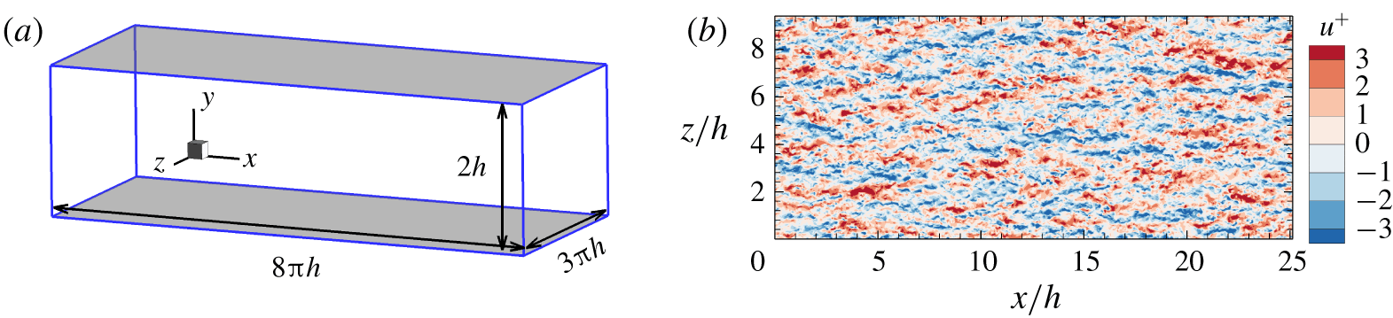
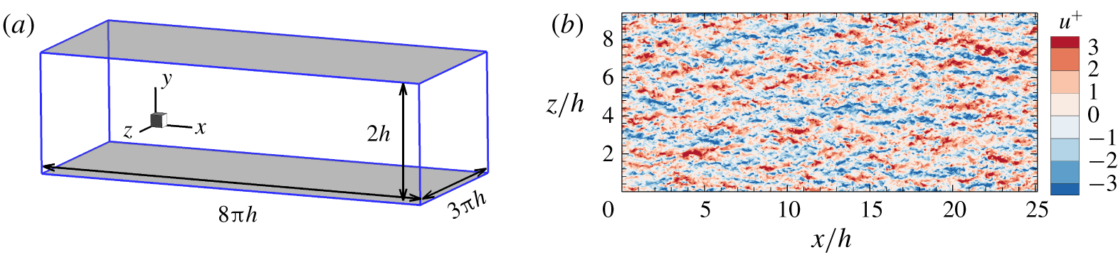
(a) Schematic of the numerical set-up of a turbulent channel flow at  $Re_{\unicode[STIX]{x1D70F}}=550$. (b) Instantaneous fluctuations of the streamwise velocity component on the
 $x{-}z$ plane at
 $y^{+}=92$.
4 Numerical validation
We use DNS data of turbulent channel flows at  $Re_{\unicode[STIX]{x1D70F}}\equiv u_{\unicode[STIX]{x1D70F}}h/\unicode[STIX]{x1D708}=550$ to validate the LMW model, where
 $u_{\unicode[STIX]{x1D70F}}$ is the friction velocity,
 $2h$ is the height of the channel and
 $\unicode[STIX]{x1D708}$ is the kinematic viscosity. The bulk Reynolds number
 $Re\equiv U_{b}h/\unicode[STIX]{x1D708}$ is approximately 10 000, where
 $U_{b}$ is the bulk velocity. The numerical set-up is sketched in figure 3(a). The computational domain is chosen to be
 $8\unicode[STIX]{x03C0}h$ in the streamwise direction (
 $x$) and
 $3\unicode[STIX]{x03C0}h$ in the spanwise direction (
 $z$). The grid numbers 1536 × 256 × 1152 are used in the streamwise (
 $x$), wall-normal (
 $y$) and spanwise (
 $z$) directions, respectively. The streamwise and spanwise resolutions are
 $\unicode[STIX]{x1D6E5}_{x}^{+}=8.95$ and
 $\unicode[STIX]{x1D6E5}_{z}^{+}=4.47$ (‘
 $+$’ indicates normalization with wall units), respectively. The minimum and maximum wall-normal resolutions are
 $\min (\unicode[STIX]{x1D6E5}_{y}^{+})=0.04$ near the wall and
 $\max (\unicode[STIX]{x1D6E5}_{y}^{+})=6.67$ at the centre of the channel. Periodic boundary conditions are used in the streamwise and spanwise directions, and no-slip boundary conditions are employed at the bottom and top walls. A pseudo-spectral method is adopted to numerically solve the Navier–Stokes equations. Time is advanced via a third-order, stiffly stable scheme. The time step is taken as
 $\unicode[STIX]{x0394}t=1.25\times 10^{-3}h/U_{b}$ (
 $\unicode[STIX]{x0394}t^{+}\approx 0.037$). The Navier–Stokes solver used in the present study has been validated in previous studies (Deng & Xu Reference Deng and Xu2012; Geng et al. Reference Geng, He, Wang, Xu, Lozano-Durán and Wallace2015; Wu et al. Reference Wu, Geng, Yao, Xu and He2017). The mean streamwise velocity profile and turbulence intensities are consistent with those of Del Álamo & Jiménez (Reference Del Álamo and Jiménez2003) at the same Reynolds number. Figure 3(b) shows instantaneous fluctuations of the streamwise velocity component on the
 $x{-}z$ plane at
 $y^{+}=92$.
The dataset was stored at every eight time steps during a period of  $20.48h/U_{b}$ as the flow reached a statistically stationary state. To calculate the temporal Fourier mode of the velocity fluctuations
 $u(x,t;y,z)$ at a given wall-normal coordinate
 $y$ and spanwise coordinate
 $z$, we divide the dataset into overlapping intervals in the time domain with a 50 % overlap and use the Hanning window to minimize spectral leakage. This leads to
 $$\begin{eqnarray}\hat{u} (x,\unicode[STIX]{x1D714};y,z)=\frac{1}{\sqrt{T\int _{0}^{T}w(t)^{2}\text{d}t}}\int _{0}^{T}w(t)u(x,t;y,z)\text{e}^{\text{i}\unicode[STIX]{x1D714}t}\,\text{d}t,\end{eqnarray}$$
where  $w(t)$ is the Hanning window, and
 $T$ is the interval length taken as
 $T=5.12h/U_{b}$ in the present calculations. The temporal energy spectrum is calculated by
 $$\begin{eqnarray}\unicode[STIX]{x1D6F7}_{t}(\unicode[STIX]{x1D714};y)=\frac{\langle \hat{u} ^{\ast }(x,\unicode[STIX]{x1D714};y,z)\hat{u} (x,\unicode[STIX]{x1D714};y,z)\rangle }{\unicode[STIX]{x0394}\unicode[STIX]{x1D714}},\end{eqnarray}$$
where  $\unicode[STIX]{x0394}\unicode[STIX]{x1D714}=2\unicode[STIX]{x03C0}/T$, and the angular bracket denotes the ensemble average which is performed in time and in the streamwise and spanwise directions due to homogeneity. The space–time Fourier mode
 $\tilde{u} (k_{x},\unicode[STIX]{x1D714};y,z)$ is determined by
 $$\begin{eqnarray}\tilde{u} (k_{x},\unicode[STIX]{x1D714};y,z)=\frac{1}{L_{x}}\int _{0}^{L_{x}}\hat{u} (x,\unicode[STIX]{x1D714};y,z)\text{e}^{-\text{i}k_{x}x}\,\text{d}x.\end{eqnarray}$$
It is noted that no window is used in the periodic streamwise direction. The space–time energy spectrum  $\unicode[STIX]{x1D6F7}(k_{x},\unicode[STIX]{x1D714};y)$ is calculated by
 $$\begin{eqnarray}\unicode[STIX]{x1D6F7}(k_{x},\unicode[STIX]{x1D714};y)=\frac{\langle \tilde{u} ^{\ast }(k_{x},\unicode[STIX]{x1D714};y,z)\tilde{u} (k_{x},\unicode[STIX]{x1D714};y,z)\rangle }{\unicode[STIX]{x0394}k_{x}\unicode[STIX]{x0394}\unicode[STIX]{x1D714}},\end{eqnarray}$$
where  $\unicode[STIX]{x0394}k_{x}=2\unicode[STIX]{x03C0}/L_{x}$, and the angular bracket denotes the ensemble average which is performed in time and in the spanwise direction. In the calculations of the LW and LMW models,
 $\unicode[STIX]{x0394}x$ is taken to be the same as the streamwise mesh size
 $\unicode[STIX]{x1D6E5}_{x}$. The numerical technique used in this section has been verified in our previous study (Wu et al. Reference Wu, Geng, Yao, Xu and He2017).
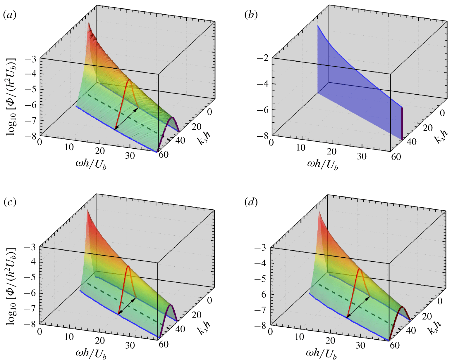
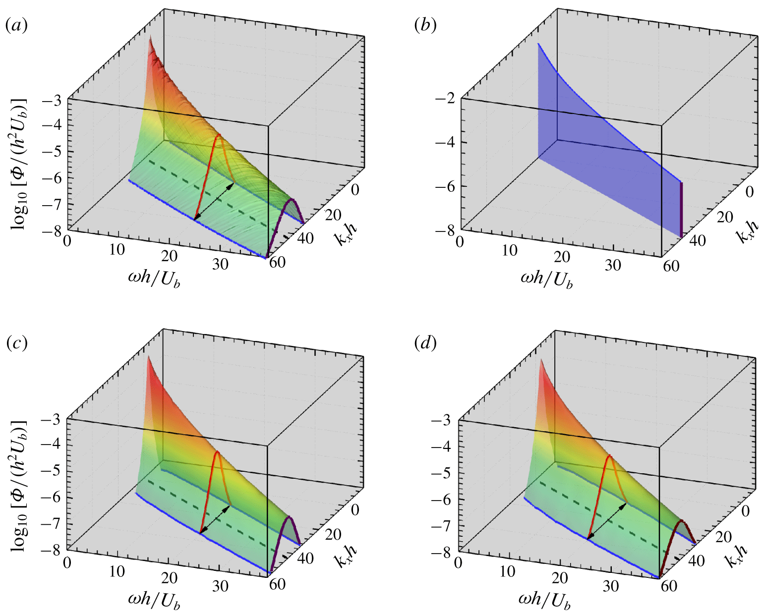
Space–time energy spectra of the streamwise velocity fluctuations at  $y^{+}=92$ in turbulent channel flows at
 $Re_{\unicode[STIX]{x1D70F}}=550$. The coloured surfaces show the energy spectra from (a) the DNS, (b) Taylor’s frozen-flow hypothesis, (c) the LW model and (d) the LMW model.
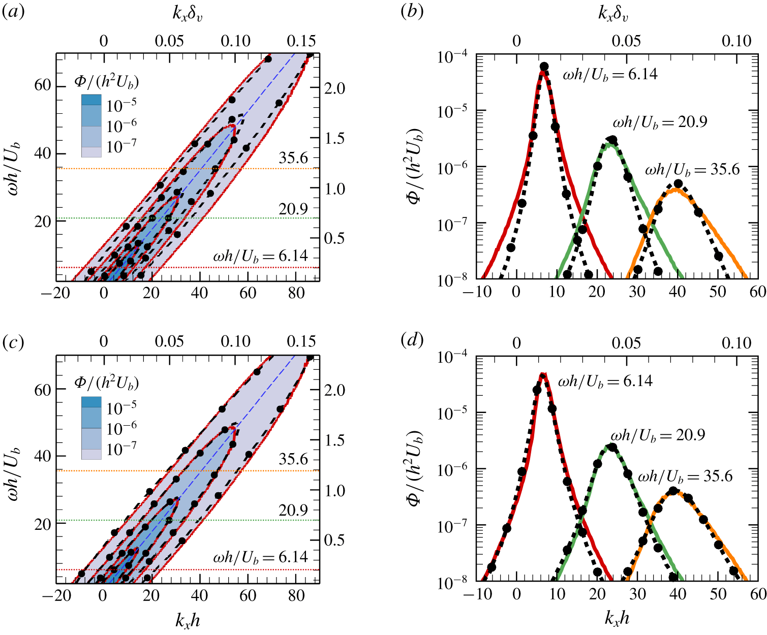
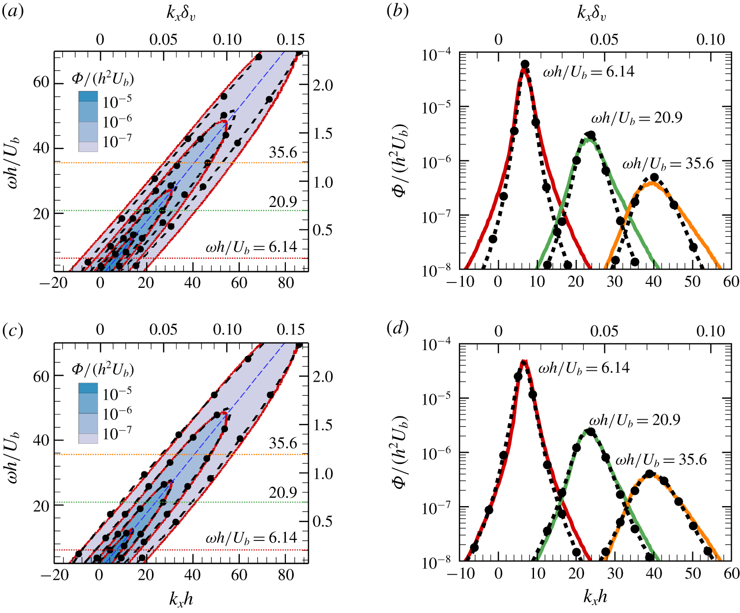
Comparison of the space–time energy spectra obtained from the DNS, the LW model and the LMW model for streamwise velocity fluctuations at  $y^{+}=92$ in turbulent channel flows at
 $Re_{\unicode[STIX]{x1D70F}}=550$. (a) Contours obtained from the DNS (coloured shades with solid lines) and the LW model (dashed lines with dots). (b) Cuts through space–time energy spectra at three different frequencies obtained from the DNS (coloured solid lines) and the LW model (dashed lines with dots). (c) Contours obtained from the DNS (coloured shades with solid lines) and the LMW model (dashed lines with dots). (d) Cuts through space–time energy spectra at three different frequencies obtained from the DNS (coloured solid lines) and the LMW model (dashed lines with dots).
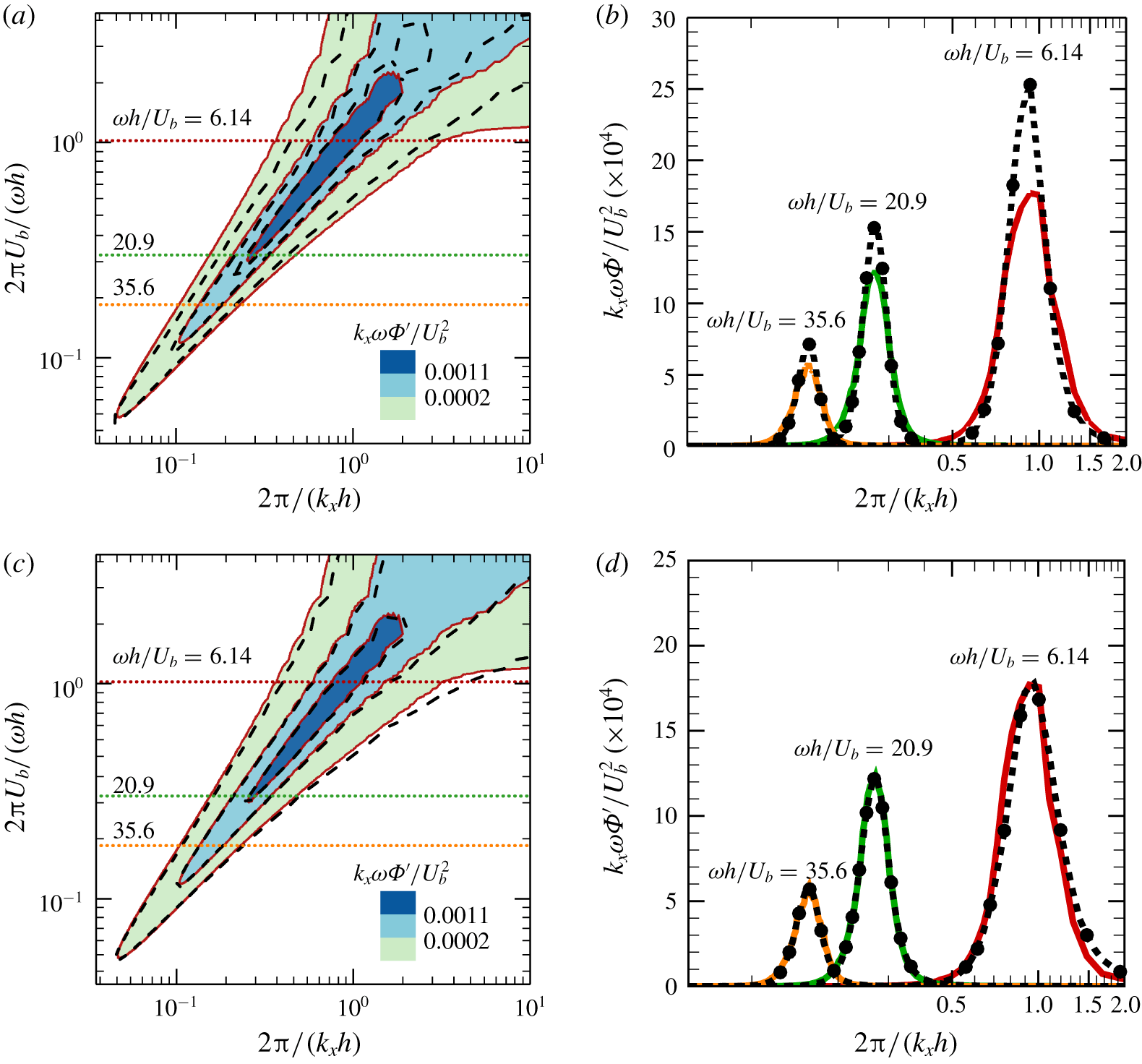
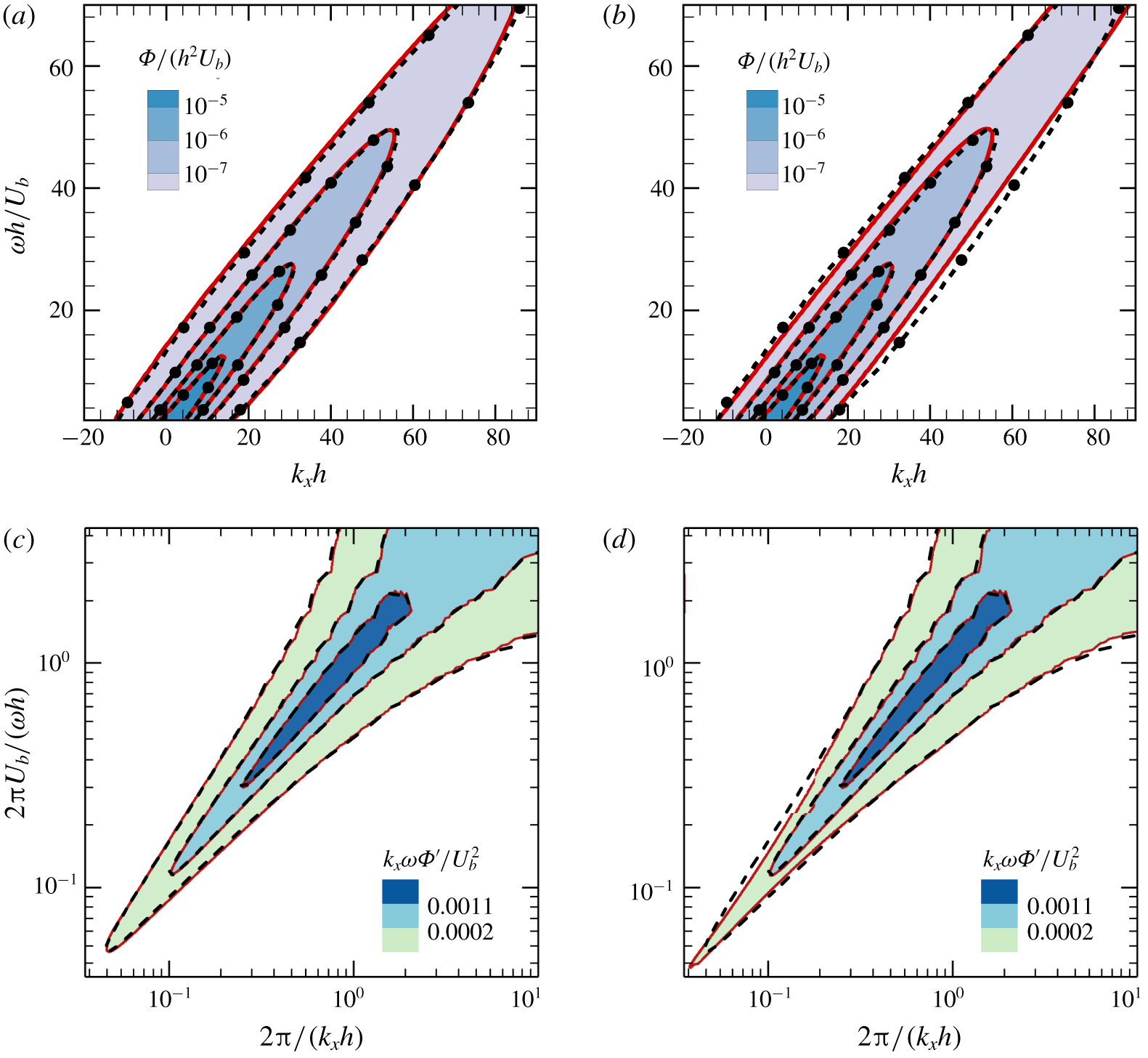
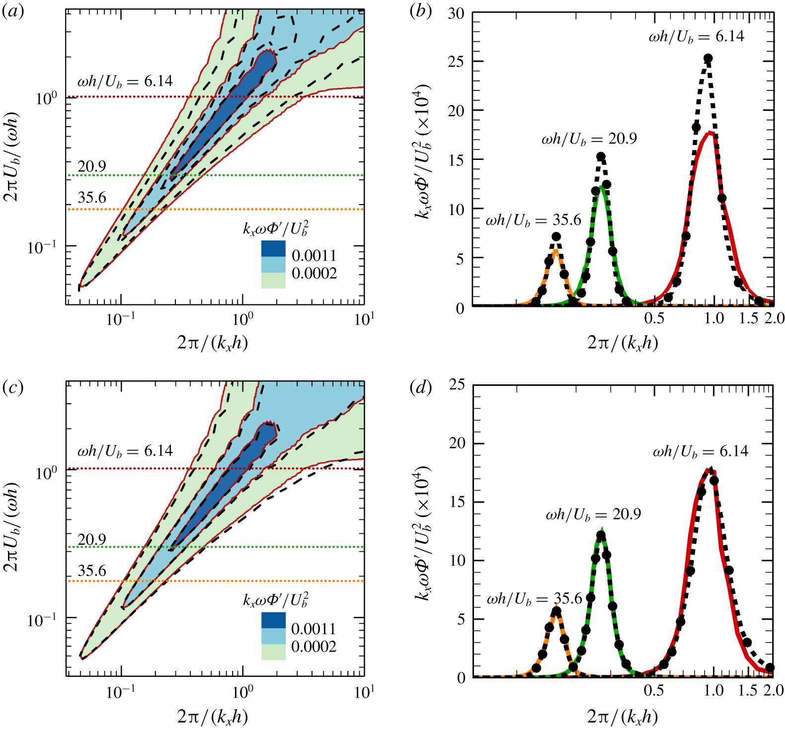
Comparison of the space–time energy spectra in ‘premultiplied’ form obtained from the DNS, the LW model and the LMW model for streamwise velocity fluctuations at  $y^{+}=92$ in turbulent channel flows at
 $Re_{\unicode[STIX]{x1D70F}}=550$. (a) Contours obtained from the DNS (coloured shades with solid lines) and the LW model (dashed lines). (b) Cuts through space–time energy spectra in ‘premultiplied’ form at three different frequencies obtained from the DNS (coloured solid lines) and the LW model (dashed lines with dots). (c) Contours obtained from the DNS (coloured shades with solid lines) and the LMW model (dashed lines). (d) Cuts through space–time energy spectra in ‘premultiplied’ form at three different frequencies obtained from the DNS (coloured solid lines) and the LMW model (dashed lines with dots).
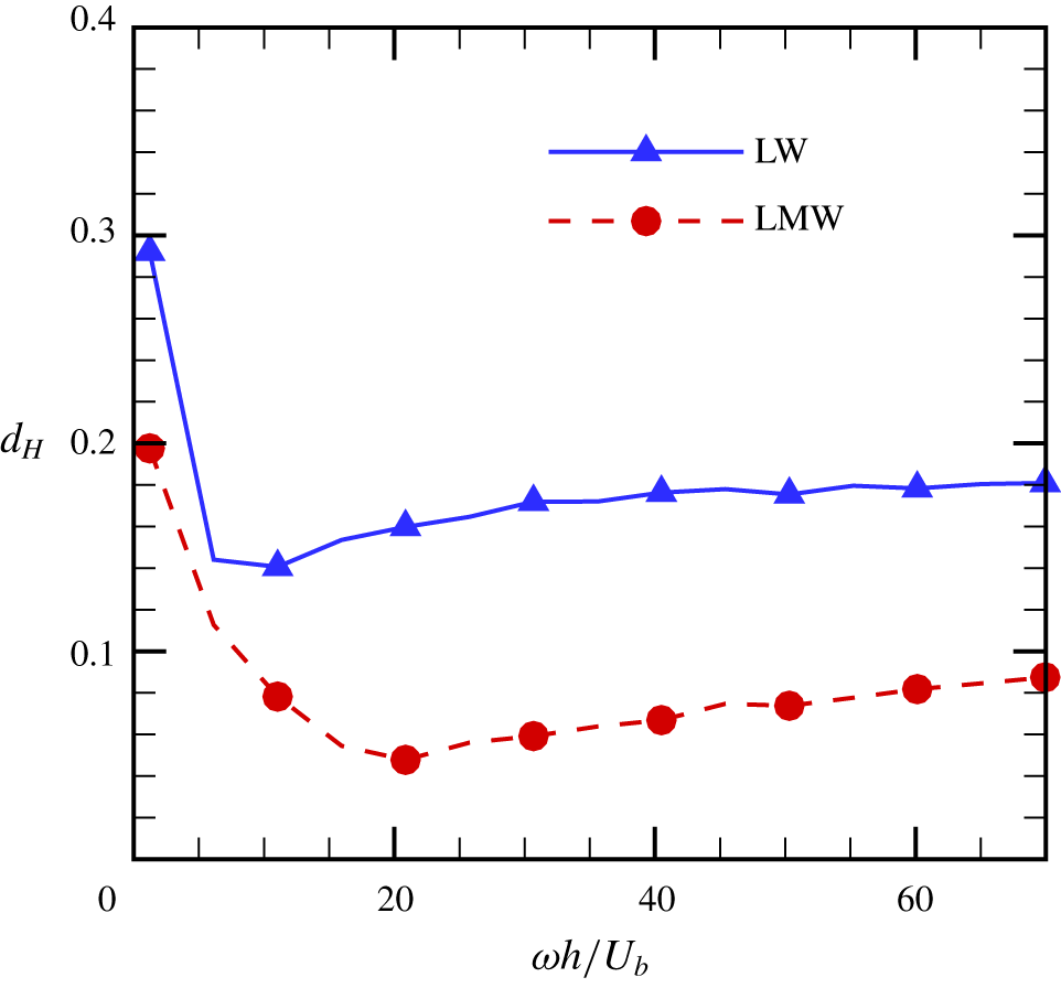
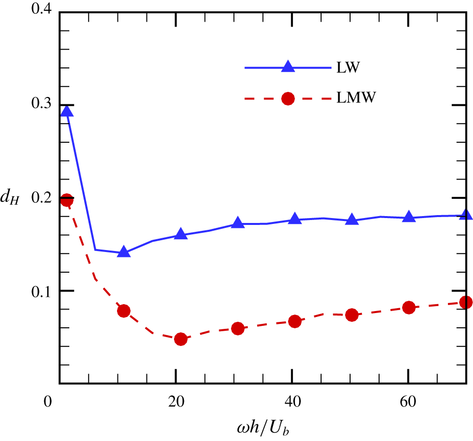
The Hellinger distances between the models and the DNS results at different frequencies.
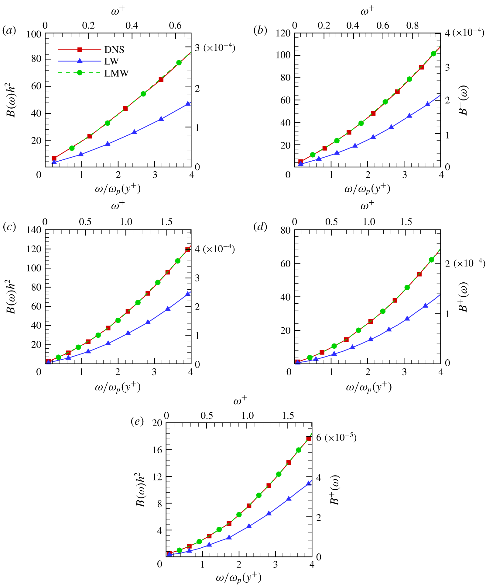
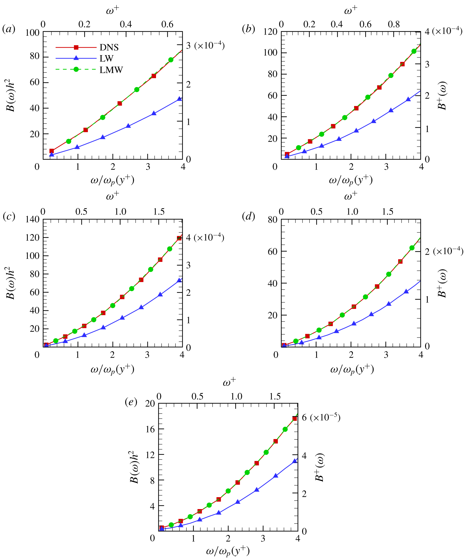
Bandwidths of the conditional distributions of the space–time energy spectra at the given frequencies for streamwise velocity fluctuations in turbulent channel flows at  $Re_{\unicode[STIX]{x1D70F}}=550$. The results from the DNS are denoted by red lines with squares, the results from the LW model are denoted by blue lines with triangles and the results from the LMW model are denoted by green lines with circles. (a)
 $y^{+}=5$. (b)
 $y^{+}=12$. (c)
 $y^{+}=44$. (d)
 $y^{+}=92$. (e)
 $y^{+}=270$. Note that the frequencies are normalized by the peak frequency
 $\unicode[STIX]{x1D714}_{p}(y^{+})$ of the dissipation spectrum
 $\unicode[STIX]{x1D714}^{2}\unicode[STIX]{x1D6F7}_{t}(\unicode[STIX]{x1D714};y^{+})$.
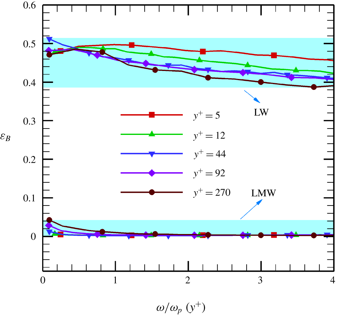
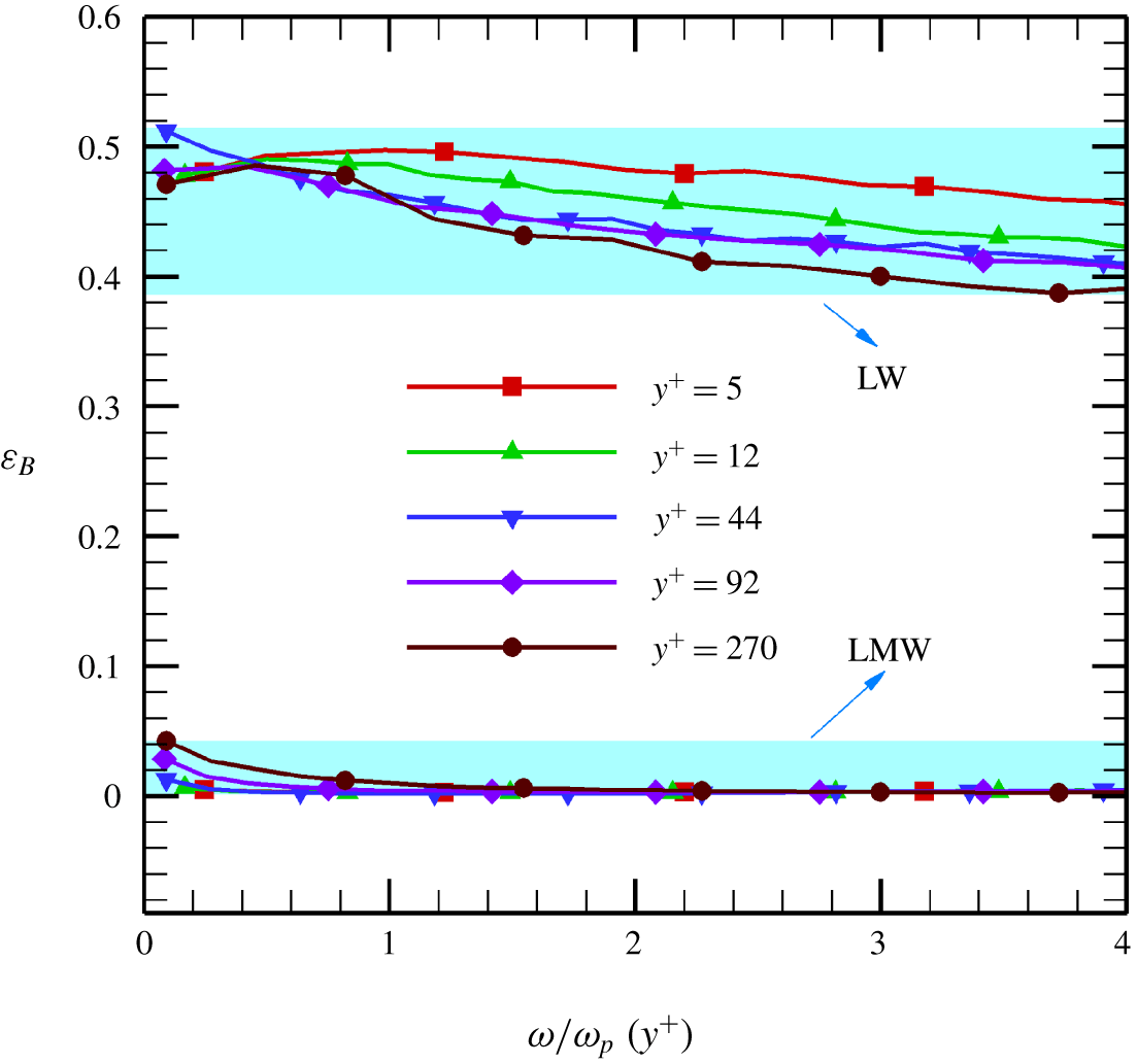
Relative errors of the spectral bandwidths between the DNS and the LW and LMW models for the streamwise velocity fluctuations in turbulent channel flows at  $Re_{\unicode[STIX]{x1D70F}}=550$. Upper band: the relative errors of the LW model. Lower band: the relative errors of the LMW model. Note that the frequencies are normalized by the peak frequency
 $\unicode[STIX]{x1D714}_{p}(y^{+})$ of the dissipation spectrum
 $\unicode[STIX]{x1D714}^{2}\unicode[STIX]{x1D6F7}_{t}(\unicode[STIX]{x1D714};y^{+})$.
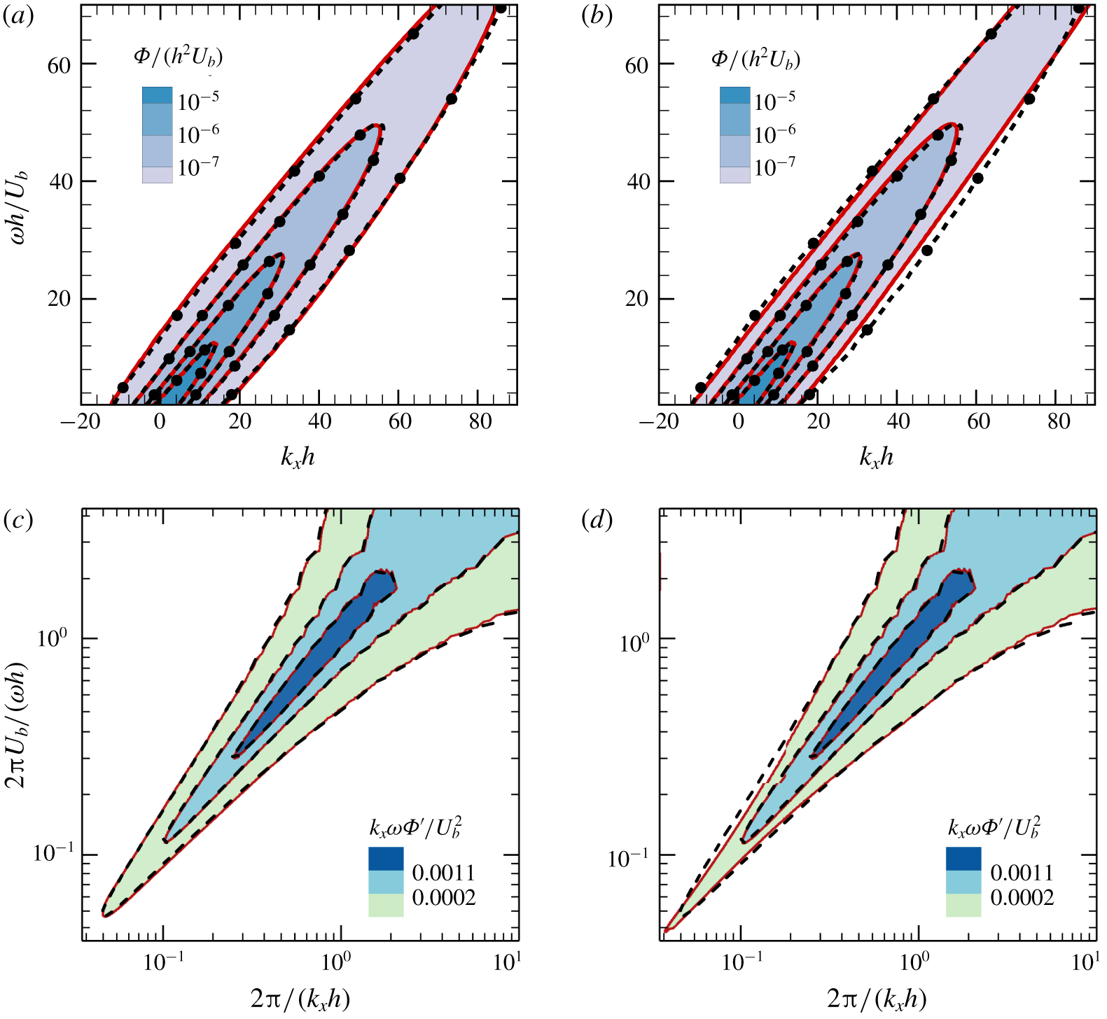
Space–time energy spectra reconstructed from the LMW model at different separations  $\unicode[STIX]{x0394}x$ (coloured shades with solid lines) compared with the result at
 $\unicode[STIX]{x0394}x=\unicode[STIX]{x0394}_{x}$. (a) Contours obtained at
 $\unicode[STIX]{x0394}x=10\unicode[STIX]{x0394}_{x}$ (
 $\unicode[STIX]{x0394}x^{+}=89.5$) compared with the result at
 $\unicode[STIX]{x0394}x=\unicode[STIX]{x1D6E5}_{x}$ (dashed lines with dots). (b) Contours obtained at
 $\unicode[STIX]{x0394}x=20\unicode[STIX]{x0394}_{x}$ (
 $\unicode[STIX]{x0394}x^{+}=179$) compared with the result at
 $\unicode[STIX]{x0394}x=\unicode[STIX]{x0394}_{x}$ (dashed lines with dots). (c) Contours of the space–time energy spectra in ‘premultiplied’ form obtained at
 $\unicode[STIX]{x0394}x=10\unicode[STIX]{x0394}_{x}$ (
 $\unicode[STIX]{x0394}x^{+}=89.5$) compared with the result at
 $\unicode[STIX]{x0394}x=\unicode[STIX]{x0394}_{x}$ (dashed lines). (d) Contours of the space–time energy spectra in ‘premultiplied’ form obtained at
 $\unicode[STIX]{x0394}x=20\unicode[STIX]{x0394}_{x}$ (
 $\unicode[STIX]{x0394}x^{+}=179$) compared with the result at
 $\unicode[STIX]{x0394}x=\unicode[STIX]{x0394}_{x}$ (dashed lines).
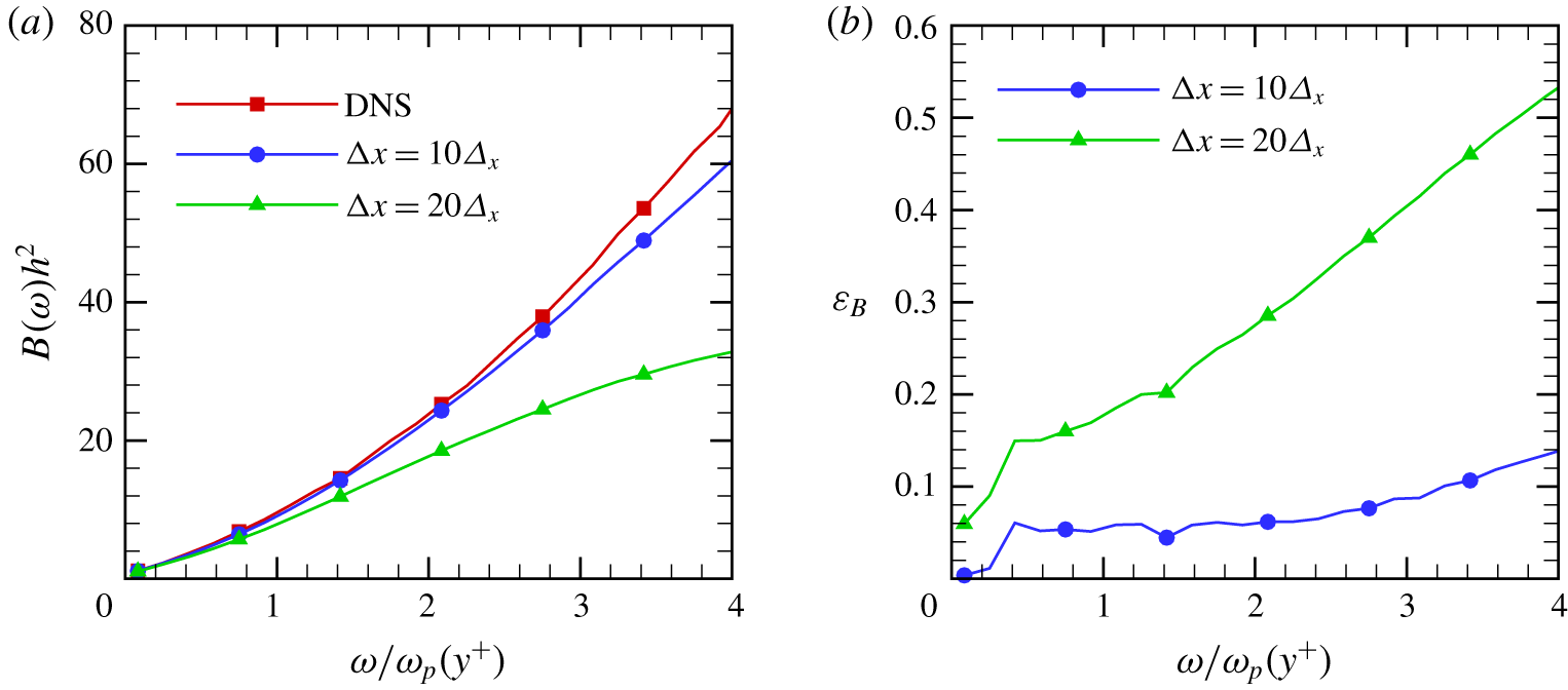
(a) Bandwidths and (b) the relative errors of the bandwidths of the space–time energy spectra reconstructed from the LMW model at  $\unicode[STIX]{x0394}x=10\unicode[STIX]{x0394}_{x}$ (
 $\unicode[STIX]{x0394}x^{+}=89.5$) and
 $\unicode[STIX]{x0394}x=20\unicode[STIX]{x1D6E5}_{x}$ (
 $\unicode[STIX]{x0394}x^{+}=179$).
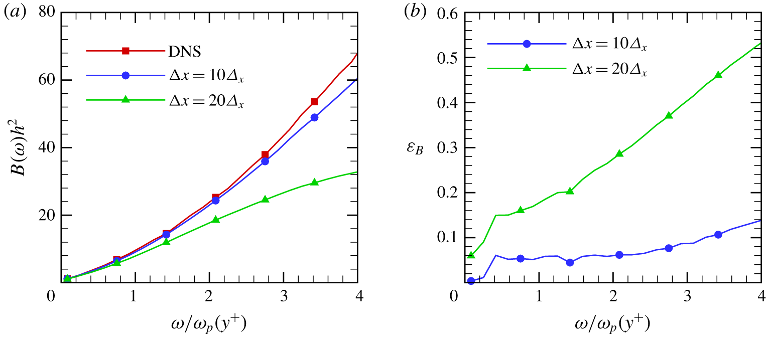
Figure 4 shows the space–time energy spectra at  $y^{+}=92$ in the logarithmic region of turbulent channel flows obtained from the DNS and three different models. The two-dimensional surface of the space–time energy spectrum plotted in figure 4(a) is narrow and mountain-like. It decays most slowly along the ridge line and has a bell-shaped slice (denoted by the red solid line) at a fixed frequency. The projection of the ridge line onto the
 $\unicode[STIX]{x1D714}-k_{x}$ plane is the characteristic line
 $\unicode[STIX]{x1D714}-k_{xc}U_{c}=0$ (denoted by the black dashed line), which relates the mean wavenumbers
 $k_{xc}$ with the frequencies
 $\unicode[STIX]{x1D714}$ through the convection velocity
 $U_{c}$. The width of the slice (denoted by the arrow line) indicates the spectral bandwidths of the conditional distribution of the energy density at a given frequency. It can be clearly observed from figure 4(b) that Taylor’s frozen-flow model displays the same characteristic line and vanishing bandwidth. The two-dimensional surfaces in figures 4(c) and 4(d) look similar to the one in figure 4(a). All three surfaces present the same ridge lines. However, the bandwidth of the slice in figure 4(c) is narrower than that of the slice in figure 4(a). The bandwidth of the slice in figure 4(d) is in agreement with that of the slice in figure 4(a). These observations are consistent with the results from the LW model and LMW model. We will quantify the differences in spectral bandwidths in figures 8 and 9.
Figures 5(a) and 5(c) compare the contours of space–time energy spectra at  $y^{+}=92$ from the DNS, the LW model and the LMW model. Wavenumbers and frequencies are also normalized by wall units, wherein
 $\unicode[STIX]{x1D6FF}_{\unicode[STIX]{x1D708}}\equiv \unicode[STIX]{x1D708}/u_{\unicode[STIX]{x1D70F}}$ is the viscous length scale. It is observed that their shapes are very similar. However, the line contours from the LW model are located within those from the DNS. The line contours from the LMW model are in good agreement with those from the DNS. In figures 5(b) and 5(d), we further compare slices of the space–time energy spectra at three different frequencies from the DNS, the LW model and the LMW model. The shapes of the curves are very similar. However, the slices from the LMW model are closer to those from the DNS than those from the LW model. In other words, the LMW model presents more spreading in the slices than does the LW model, which is in agreement with the discussion in § 2. Wu et al. (Reference Wu, Geng, Yao, Xu and He2017) use the rescaling technique in combination with the LW model to obtain the space–time energy spectra. However, the rescaling technique needs the exact value of the spectral bandwidth a priori. The LMW model does not need this value for spectral bandwidths.
Figures 6(a) and 6(c) compare the contours of the premultiplied spectra of energy density at  $y^{+}=92$ from the DNS, the LW model and the LMW model. The premultiplied spectrum for the space–time energy spectrum is defined as
 $$\begin{eqnarray}k_{x}\unicode[STIX]{x1D714}\unicode[STIX]{x1D6F7}^{\prime }(k_{x},\unicode[STIX]{x1D714})=k_{x}\unicode[STIX]{x1D714}[\unicode[STIX]{x1D6F7}(k_{x},\unicode[STIX]{x1D714})+\unicode[STIX]{x1D6F7}(-k_{x},\unicode[STIX]{x1D714})].\end{eqnarray}$$
This is consistent with the integral of the space–time energy spectra over the whole range of frequencies and wavenumbers
 $$\begin{eqnarray}\int _{-\infty }^{+\infty }\int _{-\infty }^{+\infty }\unicode[STIX]{x1D6F7}(k_{x},\unicode[STIX]{x1D714})\,\text{d}k_{x}\,\text{d}\unicode[STIX]{x1D714}=2\int _{0}^{+\infty }\int _{0}^{+\infty }k_{x}\unicode[STIX]{x1D714}[\unicode[STIX]{x1D6F7}(k_{x},\unicode[STIX]{x1D714})+\unicode[STIX]{x1D6F7}(-k_{x},\unicode[STIX]{x1D714})]\,\text{d}(\text{ln}k_{x})\,\text{d}(\text{ln}\unicode[STIX]{x1D714}).\end{eqnarray}$$
It is observed that the line contours of the premultiplied spectra from the LMW model are closer to the DNS results than those from the LW model. In figures 6(b) and 6(d), we further compare the slices of the premultiplied spectra at three different frequencies from the DNS, the LW model and the LMW model. The slices from the LMW model are in good agreement with those from the DNS. However, the peaks from the LW model overshoot those from the DNS. Therefore, the LMW model better represents the energetic flow structures than does the LW model.
To quantify the differences between the models and the DNS results, we compare the Hellinger distance between the conditional spectral distributions from the models and the DNS. The Hellinger distance (Gibbs & Su Reference Gibbs and Su2002; Liese & Vajda Reference Liese and Vajda2006) is defined as the total of the point-to-point differences between the models and the DNS results, which is given by
 $$\begin{eqnarray}d_{H}(\unicode[STIX]{x1D6F7}^{model},\unicode[STIX]{x1D6F7}^{DNS})=\left[\int \left(\sqrt{\unicode[STIX]{x1D6F7}^{model}(k_{x}|\unicode[STIX]{x1D714})}-\sqrt{\unicode[STIX]{x1D6F7}^{DNS}(k_{x}|\unicode[STIX]{x1D714})}\right)^{2}\,\text{d}k_{x}\right]^{1/2}.\end{eqnarray}$$
The Hellinger distance  $d_{H}=0$ if and only if
 $\unicode[STIX]{x1D6F7}^{model}=\unicode[STIX]{x1D6F7}^{DNS}$. As shown in figure 7, the Hellinger distances between the LMW model and the DNS results are smaller than those between the LW model and the DNS results, which implies that the LMW model is better than the LW model.
Figure 8 shows the bandwidths of the space–time energy spectra obtained from the DNS, the LW model and the LMW model at five different heights in the channel. These heights cover the typical wall layers from the viscous sublayer to the outer layer. The frequencies in the present figures are normalized using the peak frequency  $\unicode[STIX]{x1D714}_{p}(y^{+})$ of the dissipation spectra
 $\unicode[STIX]{x1D714}^{2}\unicode[STIX]{x1D6F7}_{t}(\unicode[STIX]{x1D714};y^{+})$, since the characteristic frequencies in different wall layers are not the same. For all heights in the channel, the bandwidths increase with increasing frequencies. We again find that the results from the LMW model are in good agreement with those from the DNS. However, the results from the LW model are significantly smaller than those from the DNS.
Figure 9 shows the errors in the bandwidths,  $\unicode[STIX]{x1D700}_{B}=|B^{model}-B^{DNS}|/B^{DNS}$, obtained from the LW model and the LMW model relative to the DNS results at the five different heights in the channel. The relative errors of the LW model remain between 40 % and 50 %. The relative errors in the bandwidths obtained from the LMW model are almost zero, which again demonstrates the effectiveness of the LMW model. The nominator of the relative error that is the absolute error must be bounded by a constant since the LMW model exactly predicts the spectral bandwidths. Meanwhile, the denominator of the relative error that is the spectral bandwidth decreases at lower frequencies. Therefore, their ratio becomes larger at lower frequencies.
In figures 10 and 11, the effects of the separation distance  $\unicode[STIX]{x0394}x$ between two measurement locations on the accuracy of the LMW model are investigated using the DNS data at
 $y^{+}=92$. Figures 10(a) and 10(b) compare the contours of space–time energy spectra from the LMW model at different separations
 $\unicode[STIX]{x0394}x$ with the result at
 $\unicode[STIX]{x0394}x=\unicode[STIX]{x1D6E5}_{x}$. The result with
 $\unicode[STIX]{x0394}x=10\unicode[STIX]{x1D6E5}_{x}$ (
 $\unicode[STIX]{x0394}x^{+}=89.5$) is better than that with
 $\unicode[STIX]{x0394}x=20\unicode[STIX]{x1D6E5}_{x}$ (
 $\unicode[STIX]{x0394}x^{+}=179$). As expected, the accuracy of the LMW model becomes better with decreasing separation distance. Figures 10(c) and 10(d) compare the contours of the premultiplied spectra of energy density at different separations
 $\unicode[STIX]{x0394}x$ with the result at
 $\unicode[STIX]{x0394}x=\unicode[STIX]{x1D6E5}_{x}$. The results obtained are in consistent with figures 10(a) and 10(b). It can be observed from figure 11(a) that the spectral bandwidths at
 $\unicode[STIX]{x0394}x=10\unicode[STIX]{x1D6E5}_{x}$ are close to the DNS results, while the spectral bandwidths at
 $\unicode[STIX]{x0394}x=20\unicode[STIX]{x1D6E5}_{x}$ deviate from the DNS results. The relative errors of the LMW model shown in figure 11(b) are consistent with figures 10 and 11(a). It is noted that the relative error is less than 10 % for low and moderate frequencies at the separation distance
 $\unicode[STIX]{x0394}x=10\unicode[STIX]{x1D6E5}_{x}$ (
 $\unicode[STIX]{x0394}x^{+}=89.5$).
5 Conclusions and future work
We develop a statistical model for reconstructing space–time energy spectra in turbulent flows. It is shown that this model can exactly predict the mean wavenumbers and spectral bandwidths of the space–time energy spectra. Both Taylor’s frozen-flow model and the LW model can predict the mean wavenumbers. However, the former incorrectly predicts the spectral bandwidths to be zero, and the latter excludes the contributions of amplitude derivatives, thus significantly under-predicting the spectral bandwidths. It is noted that the LW model uses the amplitudes as weights but does not explicitly use the amplitude derivatives. Instead, the present model includes both phase and amplitude derivatives so that it can correctly predict the mean wavenumbers and spectral bandwidths.
The LMW model can be used to numerically reconstruct space–time energy spectra from an incomplete dataset in physical space. The dataset required for the LMW model is the time series of velocity fluctuations at a finite number of measurement points, wherein extensive spatial sampling is not needed. As an analytical example, a propagating Gaussian signal modulated by a non-propagating Gaussian function is designed to illustrate the LMW model. Furthermore, the DNS of turbulent channel flows is performed to verify the LMW model. All the results validate the LMW model.
Taylor’s frozen-flow hypothesis proposed a physical picture for turbulent passages, in which the spatial patterns of turbulent motions are carried past a fixed point at the convection velocity without significantly changing. The hypothesis highlights an attack line to reconstruct space–time energy spectra of turbulent flows. As a first approximation, flow patterns are assumed to be local waves, which leads to the LW model. The present paper suggests a second approximation, in which the energetic flow patterns are represented by local modulated waves, such that the proposed model can exactly predict the spectral bandwidths. Wavepackets that include more wavenumbers can provide a higher approximation of the space–time energy spectra.
Acknowledgements
This work is supported by NSFC Basic Science Center Program for ‘Multiscale Problems in Nonlinear Mechanics’ (no. 11988102) and National Natural Science Foundation of China (nos 11232011 and 11572331). The authors would like to acknowledge the support from the Strategic Priority Research Program (grant no. XDB22040104) and the Key Research Program of Frontier Sciences of the Chinese Academy of Sciences (grant no. QYZDJ-SSW-SYS002).
Declaration of interests
The authors report no conflict of interest.