1. Introduction
The magnetosphere is a region near an astronomical object where the plasma interacts with the magnetic field of the object. In the case of Earth, its magnetic field is deformed by the solar wind, which is an ‘ionized gas’ with a very large electrical conductivity, chiefly made up of protons and electrons moving at high velocities (Ratcliffe Reference Ratcliffe1972). The study of the terrestrial magnetosphere is very important, since it protects Earth’s surface, satellites, telecommunication systems and, in general, electric power grids, from the hot and highly conductive solar wind (Lyon Reference Lyon2000; Shi et al. Reference Shi, Zong, Fu, Dunlop, Pu, Parks, Wei, Li, Zhang and Nowada2013).
Magnetic fields in the presence of plasmas are governed by the magnetohydrodynamics (MHD) equations. Finding steady-state solutions of these equations is very useful as a starting point in the study of magnetic and plasma instabilities. However, it is well known that analytical solutions to the MHD equations are rare and that in most practical problems the known solutions are not applicable. There are in fact many analytical solutions based on the Grad–Shafranov equations (Grad & Rubin Reference Grad and Rubin1958; Shafranov Reference Shafranov1966) for the case of toroidal plasmas in a tokamak, but these are mostly two-dimensional due to the symmetry of the problem.
Numerical solutions are relatively easy to obtain; however, to solve many theoretical and experimental problems in magnetospheric physics, magnetic field models are in general needed and can offer better understanding of the underlying physics. There are some quantitative models for the external geomagnetic field (Sergeev & Tsyganenko Reference Sergeev and Tsyganenko1980; Voigt Reference Voigt1981; Tsyganenko Reference Tsyganenko1990; Jordan Reference Jordan1994; Stern Reference Stern1994; Hilmer & Voigt Reference Hilmer and Voigt1995; Romashchenko & Reshetnikov Reference Romashchenko and Reshetnikov2000; Siscoe Reference Siscoe2001), which are widely used for various purposes by the magnetospheric research community. At least two kinds of models can be distinguished. The first class of models is based on experimental observations (Alexeev Reference Alexeev1978; Tsyganenko & Usmanov Reference Tsyganenko and Usmanov1982; Stern Reference Stern1985; Tsyganenko Reference Tsyganenko1987, Reference Tsyganenko1989, Reference Tsyganenko2002); these models are constructed by minimising the discrepancy between model outputs and satellite observations, and they describe the magnetosphere accurately. For the second class of models (Sergeev & Tsyganenko Reference Sergeev and Tsyganenko1980; Voigt Reference Voigt1981; Hilmer & Voigt Reference Hilmer and Voigt1995; Willis, Holder & Davis Reference Willis, Holder and Davis1999; Romashchenko & Reshetnikov Reference Romashchenko and Reshetnikov2000; Stadelmann et al. Reference Stadelmann, Vogt, Glassmeier, Kallenrode and Voigt2010), a potential field approach is used to model the magnetic effect of the Chapman–Ferraro currents on the magnetopause; these models can be used to assess magnetospheric configurations which differ significantly from the magnetosphere of present-day Earth. For example, the potential field model approach has been successfully used to model the magnetosphere of other planets (Voigt, Behannon & Ness Reference Voigt, Behannon and Ness1987; Voigt & Ness Reference Voigt and Ness1990).
The potential field approach is based on the shape of the magnetopause and the parameters of the internal field. Therefore, it considers the Chapman–Ferraro currents as input configurations rather than as coming from theoretical predictions. This model is appropriate for studying the actual configuration of magnetospheres based on observational data, but it cannot be used to study their origin since the model assumes a configuration that already exists. In fact, a theoretical model capable of reproducing the interaction between the solar wind and an intrinsic magnetosphere from first principles has not been developed previously, to the best of our knowledge.
In this work, we propose an analytical steady solution to the MHD equations for the case of an intrinsic magnetosphere, assuming that the magnetic field is not strong enough to deviate the solar wind appreciably. For this purpose, we introduce a new electromagnetic gauge condition that simplifies the solution of the MHD equations. By applying this model to Earth and comparing its results with experimental observations, we find that the model can reproduce satisfactorily the geometrical configuration of the magnetosphere. Furthermore, our solution shows that the solar wind should have a finite conductivity. Other features, such as the Chapman–Ferrato currents, are also observed.
This paper is organised as follows: in § 2, we first solve the MHD equations by considering a magnetic dipole in the presence of moving plasma. In § 3, we substitute in experimental values for the Earth’s magnetic field and solar wind to compare deformation parameters of the terrestrial magnetosphere with experimental observations. Finally, in § 4, we analyse and discuss the results.
2. Analytical solution
We start our derivation by considering a highly conductive plasma in the presence of a magnetic field, e.g. the magnetic field generated by Earth. In this case, we know that the magnetic field should satisfy the diffusion equation (David Reference David1966; Cowling Reference Cowling1976),
 $$\begin{eqnarray}\displaystyle \frac{\partial \boldsymbol{B}}{\partial t}={\it\eta}_{m}{\rm\nabla}^{2}\boldsymbol{B}+\boldsymbol{{\rm\nabla}}\times (\boldsymbol{v}\times \boldsymbol{B}), & & \displaystyle\end{eqnarray}$$
where
 ${\it\eta}_{m}=1/{\it\mu}{\it\sigma}$
is the magnetic viscosity,
 ${\it\sigma}$
is the conductivity and
 ${\it\mu}$
is the magnetic permeability of the plasma. Most geomagnetic models assume infinite conductivity of the solar wind; however, we assume here that the conductivity is finite, and we will show later that if the plasma were to have infinite conductivity, then the terrestrial magnetosphere could not be formed.
The evolution of the plasma is obtained by solving the momentum conservation equation (David Reference David1966; Cowling Reference Cowling1976)
 $$\begin{eqnarray}\displaystyle {\it\rho}\left(\frac{\partial \boldsymbol{v}}{\partial t}+\boldsymbol{v}\boldsymbol{\cdot }\boldsymbol{{\rm\nabla}}\boldsymbol{v}\right)=-\boldsymbol{{\rm\nabla}}P+\boldsymbol{j}\times \boldsymbol{B}+{\it\eta}{\rm\nabla}^{2}\boldsymbol{v} & & \displaystyle\end{eqnarray}$$
and the continuity equation
 $$\begin{eqnarray}\displaystyle \boldsymbol{{\rm\nabla}}\boldsymbol{\cdot }({\it\rho}\boldsymbol{v})=-\frac{\partial {\it\rho}}{\partial t}. & & \displaystyle\end{eqnarray}$$
Here
 ${\it\rho}$
is the density,
 $\boldsymbol{v}$
is the velocity,
 $P$
is the hydrostatic pressure,
 ${\it\eta}$
is the shear viscosity and
 $\boldsymbol{j}$
is the electric density current. The solar wind is nearly inviscid, so in this study we will consider
 ${\it\eta}=0$
. Furthermore, we assume that the magnetic field generated by the astronomical object is not strong enough to appreciably deviate the solar wind, i.e. the plasma parameter
 ${\it\beta}\equiv 2{\it\mu}P/B^{2}\gg 1$
and therefore the forcing term
 $\boldsymbol{j}\times \boldsymbol{B}\propto B^{2}$
can be neglected. Thus, (2.2) and (2.3) form a complete set of differential equations describing the dynamics of the solar wind, and are decoupled from (2.1) for the magnetic field. Note that the opposite is not true, i.e. the magnetic diffusion equation depends on the velocity field.
In order to describe accurately the terrestrial magnetosphere, one would need to consider compressible and rotational flows and non-homogeneous velocity fields. However, an analytical solution of such a system would become impossible to achieve, and we may lose the opportunity to get physical information of the kind that is typically provided by analytical models. Therefore, we study the case where density and velocity fluctuations in the solar wind due to the magnetic field of the source are negligible; so, as a first approximation, we consider an incompressible (
 $\boldsymbol{{\rm\nabla}}\boldsymbol{\cdot }\boldsymbol{v}=0$
) and irrotational (
 $\boldsymbol{{\rm\nabla}}\times \boldsymbol{v}=0$
) fluid in the steady state,
 $\partial /\partial t=0$
. More precisely, we consider a constant velocity for the solar wind and derive an exact solution under this assumption. By doing this, we are excluding many interesting physical phenomena that occur in the magnetosphere, e.g. the dynamics related to the formation of vortices, which are generally formed in the proximity of the magnetic source, as well as magnetic reconnection processes (Frey et al.
Reference Frey, Phan, Fuselier and Mende2003; Priest & Forbes Reference Priest and Forbes2007; Mendoza & Muñoz Reference Mendoza and Muñoz2008). We will demonstrate the basic concepts of how the magnetic field of a magnetic dipole is deformed by the presence of the solar wind and characterise this deformation using typical plasma parameters, such as the velocity and electric conductivity of the solar wind. It is also of great interest to find out how closely such a simplified model can describe the geometry of the terrestrial magnetosphere.
Based on the considerations above, by using the vector potential
 $\boldsymbol{A}$
, such that
 $\boldsymbol{B}=\boldsymbol{{\rm\nabla}}\times \boldsymbol{A}$
, together with the vectorial relation
 $$\begin{eqnarray}\displaystyle \boldsymbol{{\rm\nabla}}\times (\boldsymbol{{\rm\nabla}}\times \boldsymbol{A})=\boldsymbol{{\rm\nabla}}(\boldsymbol{{\rm\nabla}}\boldsymbol{\cdot }\boldsymbol{A})-{\rm\nabla}^{2}\boldsymbol{A}, & & \displaystyle\end{eqnarray}$$
we can write (2.1) as
 $$\begin{eqnarray}{\it\eta}_{m}[\boldsymbol{{\rm\nabla}}(\boldsymbol{{\rm\nabla}}\boldsymbol{\cdot }\boldsymbol{A})-{\rm\nabla}^{2}\boldsymbol{A}]=\boldsymbol{v}\times (\boldsymbol{{\rm\nabla}}\times \boldsymbol{A}).\end{eqnarray}$$
Keeping in mind that the fluid velocity is constant, we use the identity
 $$\begin{eqnarray}\boldsymbol{v}\times (\boldsymbol{{\rm\nabla}}\times \boldsymbol{A})=\boldsymbol{{\rm\nabla}}(\boldsymbol{v}\boldsymbol{\cdot }\boldsymbol{A})-(\boldsymbol{v}\boldsymbol{\cdot }\boldsymbol{{\rm\nabla}})\boldsymbol{A}\end{eqnarray}$$
to rewrite (2.5) as
 $$\begin{eqnarray}{\it\eta}_{m}{\rm\nabla}^{2}\boldsymbol{A}-(\boldsymbol{v}\boldsymbol{\cdot }\boldsymbol{{\rm\nabla}})\boldsymbol{A}=\boldsymbol{{\rm\nabla}}({\it\eta}_{m}\boldsymbol{{\rm\nabla}}\boldsymbol{\cdot }\boldsymbol{A}-\boldsymbol{v}\boldsymbol{\cdot }\boldsymbol{A}).\end{eqnarray}$$
Note that one can also write (2.1) as
 $0={\it\eta}_{m}{\rm\nabla}^{2}\boldsymbol{B}-(\boldsymbol{v}\boldsymbol{\cdot }\boldsymbol{{\rm\nabla}})\boldsymbol{B}$
and try to solve the problem directly for the magnetic field. However, constructing a magnetospheric configuration from this solution is more difficult, since one needs to consider, besides the constraint
 $\boldsymbol{{\rm\nabla}}\boldsymbol{\cdot }\boldsymbol{B}=0$
, a dipole-like magnetic field. Therefore, we work here with the vector potential, which satisfies by construction the constraint
 $\boldsymbol{{\rm\nabla}}\boldsymbol{\cdot }\boldsymbol{B}=0$
and additionally gives us the freedom to choose a gauge condition, i.e. a relation for
 $\boldsymbol{{\rm\nabla}}\boldsymbol{\cdot }\boldsymbol{A}$
. Thus, we only need to focus on finding the dipole-like solution.
Equation (2.7) must be solved in order to know the deformation of the magnetic field due to the interaction with the solar wind. Here, we introduce an unconventional way to solve (2.7). We first set the gauge condition as
 ${\it\eta}_{m}\boldsymbol{{\rm\nabla}}\boldsymbol{\cdot }\boldsymbol{A}-\boldsymbol{v}\boldsymbol{\cdot }\boldsymbol{A}=0$
and find a solution to the equation
 $$\begin{eqnarray}\displaystyle {\it\eta}_{m}{\rm\nabla}^{2}\boldsymbol{A}-(\boldsymbol{v}\boldsymbol{\cdot }\boldsymbol{{\rm\nabla}})\boldsymbol{A}=0 & & \displaystyle\end{eqnarray}$$
for the vector potential
 $\boldsymbol{A}$
; then, we use the constraint to find the real solution, including the integration parameters. Thus, using the fact that the plasma velocity can be written as the gradient of a scalar potential,
 $\boldsymbol{v}=-\boldsymbol{{\rm\nabla}}{\it\phi}_{v}$
, and substituting this into (2.8), we obtain
 $$\begin{eqnarray}\displaystyle {\it\eta}_{m}{\rm\nabla}^{2}\boldsymbol{A}+\boldsymbol{{\rm\nabla}}{\it\phi}_{v}\boldsymbol{\cdot }\boldsymbol{{\rm\nabla}}\boldsymbol{A}=0. & & \displaystyle\end{eqnarray}$$
Let us now propose a solution of the form
 $$\begin{eqnarray}\displaystyle \boldsymbol{A}={\it\phi}_{m}\boldsymbol{A}_{0} & & \displaystyle\end{eqnarray}$$
such that, when we substitute it into (2.9), we obtain the following relation:
 $$\begin{eqnarray}{\it\eta}_{m}{\it\phi}_{m}{\rm\nabla}^{2}\boldsymbol{A}_{0}+({\it\eta}_{m}{\rm\nabla}^{2}{\it\phi}_{m}+\boldsymbol{{\rm\nabla}}{\it\phi}_{v}\boldsymbol{\cdot }\boldsymbol{{\rm\nabla}}{\it\phi}_{m})\boldsymbol{A}_{0}+(2{\it\eta}_{m}\boldsymbol{{\rm\nabla}}{\it\phi}_{m}+{\it\phi}_{m}\boldsymbol{{\rm\nabla}}{\it\phi}_{v})\boldsymbol{\cdot }\boldsymbol{{\rm\nabla}}\boldsymbol{A}_{0}=0.\end{eqnarray}$$
Note that by choosing
 $$\begin{eqnarray}\boldsymbol{{\rm\nabla}}{\it\phi}_{m}=-\frac{{\it\phi}_{m}}{2{\it\eta}_{m}}\boldsymbol{{\rm\nabla}}{\it\phi}_{v},\end{eqnarray}$$
we get the modified Helmholtz equation
 $$\begin{eqnarray}{\rm\nabla}^{2}\boldsymbol{A}_{0}-k^{2}\boldsymbol{A}_{0}=0,\end{eqnarray}$$
where
 $$\begin{eqnarray}k=\frac{1}{2{\it\eta}_{m}}\sqrt{\boldsymbol{{\rm\nabla}}{\it\phi}_{v}\boldsymbol{\cdot }\boldsymbol{{\rm\nabla}}{\it\phi}_{v}}=\frac{{\it\mu}{\it\sigma}}{2}|\boldsymbol{{\rm\nabla}}{\it\phi}_{v}|.\end{eqnarray}$$
The solution of (2.13), in spherical coordinates
 $(r,{\it\theta},{\it\phi})$
, is given in terms of the spherical harmonics,
 $Y_{lm}({\it\theta},{\it\phi})$
, and the modified spherical Bessel polynomials,
 $i_{l}(kr)$
and
 $n_{l}(kr)$
(Arfken & Weber Reference Arfken and Weber2005). Therefore, we can write the solution as
 $$\begin{eqnarray}\displaystyle \boldsymbol{A}_{0}=\mathop{\sum }_{l=0}^{\infty }\mathop{\sum }_{m=-l}^{l}[\boldsymbol{D}_{lm}n_{l}(kr)]\,Y_{lm}({\it\theta},{\it\phi}), & & \displaystyle\end{eqnarray}$$
where we have suppressed the contribution of
 $i_{l}(kr)$
since we require a converging solution for
 $r\rightarrow \infty$
. On the other hand, the solution of (2.12) can be obtained by direct integration as
 $$\begin{eqnarray}\displaystyle {\it\phi}_{m}=C_{1}\text{e}^{-{\it\phi}_{v}/2{\it\eta}_{m}}. & & \displaystyle\end{eqnarray}$$
Upon substituting both of the solutions (2.15) and (2.16) into (2.10), we can write the general solution for the potential vector as
 $$\begin{eqnarray}\displaystyle \boldsymbol{A}=\text{e}^{-{\it\phi}_{v}/2{\it\eta}_{m}}\mathop{\sum }_{l=0}^{\infty }\mathop{\sum }_{m=-l}^{l}[\boldsymbol{D}_{lm}n_{l}(kr)]\,Y_{lm}({\it\theta},{\it\phi}). & & \displaystyle\end{eqnarray}$$
Note that we have redefined the integration constant
 $C_{1}\boldsymbol{D}_{lm}\rightarrow \boldsymbol{D}_{lm}$
for simplicity.
From now on, we assume that the source of the magnetic field is magnetic dipole-like. Therefore, the only remaining terms in (2.17) are
 $$\begin{eqnarray}\displaystyle \boldsymbol{A}=\text{e}^{-{\it\phi}_{v}/2{\it\eta}_{m}-kr}\frac{M^{\prime }(1+kr)}{k^{3/2}r^{3}}(-y,x,0), & & \displaystyle\end{eqnarray}$$
where
 $M^{\prime }$
is a constant that will be related to the magnetic dipole-like moment. Note that one can also assume another kind of multipolar expansion for more general cases. In order to have a valid solution of (2.7), we impose the gauge condition
 $$\begin{eqnarray}\displaystyle {\it\eta}_{m}\boldsymbol{{\rm\nabla}}\boldsymbol{\cdot }\boldsymbol{A}+\boldsymbol{{\rm\nabla}}{\it\phi}_{v}\boldsymbol{\cdot }\boldsymbol{A}=0, & & \displaystyle\end{eqnarray}$$
which must be satisfied. For this purpose, we can include additional terms in the expansion of the solution (2.17), obtaining
 $$\begin{eqnarray}\displaystyle \boldsymbol{A}=M^{\prime }\text{e}^{-{\it\phi}_{v}/2{\it\eta}_{m}-kr}\left(-\frac{y(1+kr)}{k^{3/2}r^{3}}+\frac{1}{\sqrt{k}r}\frac{1}{|\boldsymbol{{\rm\nabla}}{\it\phi}_{v}|}\frac{\partial {\it\phi}_{v}}{\partial y},\frac{x(1+kr)}{k^{3/2}r^{3}}-\frac{1}{\sqrt{k}r}\frac{1}{|\boldsymbol{{\rm\nabla}}{\it\phi}_{v}|}\frac{\partial {\it\phi}_{v}}{\partial x},0\right). & & \displaystyle \nonumber\\ \displaystyle & & \displaystyle\end{eqnarray}$$
The constant
 $M^{\prime }$
is related to the magnetic dipole moment of the source,
 $M$
. Since for low plasma velocity we expect to recover the solution of the vector potential for a magnetic dipole, we can conclude that
 $M^{\prime }=k^{3/2}{\it\mu}M/4{\rm\pi}$
. Substituting this into (2.20) and taking into account the definition of
 $k$
in (2.14), we obtain the final solution,
 $$\begin{eqnarray}\boldsymbol{A}=\frac{{\it\mu}M}{4{\rm\pi}}\text{e}^{-{\it\phi}_{v}/2{\it\eta}_{m}-kr}\left(-\frac{y(1+kr)}{r^{3}}+\frac{{\it\mu}{\it\sigma}}{2r}\frac{\partial {\it\phi}_{v}}{\partial y},\frac{x(1+kr)}{r^{3}}-\frac{{\it\mu}{\it\sigma}}{2r}\frac{\partial {\it\phi}_{v}}{\partial x},0\right).\end{eqnarray}$$
Thus, for
 $|\boldsymbol{{\rm\nabla}}{\it\phi}_{v}|\rightarrow 0$
or
 ${\it\sigma}\rightarrow 0$
(both cases imply
 $k\rightarrow 0$
), we get the vector potential for a magnetic dipole. On the other hand, if the plasma has very high conductivity, we see that the solution decays exponentially to zero, implying that at infinite conductivity, formation of the magnetosphere becomes impossible. From (2.21), we can determine the magnetic field using the expression
 $\boldsymbol{B}=\boldsymbol{{\rm\nabla}}\times \boldsymbol{A}$
. Note that the
 $z$
component of the velocity,
 $-\partial {\it\phi}_{v}/\partial z$
, does not appear explicitly in (2.21), although it has a contribution via
 ${\it\phi}_{v}$
in the exponential term.
Our model is able to describe more general cases, e.g. multipolar terms, by including more terms in the expansion in (2.17). However, the gauge relation given by (2.19) must always be satisfied. One can find necessary conditions on the vector field
 $\boldsymbol{A}_{0}$
for the gauge relation, (2.19), and the Helmholtz equation, (2.13), to be satisfied simultaneously. By substituting
 $\boldsymbol{A}={\it\phi}_{m}\boldsymbol{A}_{0}$
into the gauge condition and performing some algebraic manipulations, one gets
 $$\begin{eqnarray}\boldsymbol{{\rm\nabla}}\boldsymbol{\cdot }\boldsymbol{A}_{0}=k\hat{v}\boldsymbol{\cdot }\boldsymbol{A}_{0},\end{eqnarray}$$
where
 $\hat{v}\equiv \boldsymbol{v}/|\boldsymbol{v}|$
. Therefore, since
 $\hat{v}$
is a constant vector, one needs lower-order terms in the expansion of
 $\boldsymbol{A}_{0}$
to fulfil this relation. In principle, one expects to always find a solution satisfying both (2.13) and (2.22) by writing
 $\boldsymbol{A}_{0}=\boldsymbol{A}_{1}+kA_{2}\hat{v}_{\bot }$
, where
 $\boldsymbol{A}_{1}$
is a vectorial field that satisfies (2.13) and
 $\boldsymbol{{\rm\nabla}}\boldsymbol{\cdot }\boldsymbol{A}_{1}=0$
,
 $A_{2}$
is a scalar such that
 ${\rm\nabla}^{2}A_{2}-k^{2}A_{2}=0$
and
 $\hat{v}_{\bot }$
is a unitary vector perpendicular to
 $\hat{v}$
. Upon substituting this solution into (2.22), we obtain
 $\hat{v}_{\bot }\boldsymbol{\cdot }\boldsymbol{{\rm\nabla}}A_{2}=\hat{v}\boldsymbol{\cdot }\boldsymbol{A}_{1}$
, and due to the fact that
 $\boldsymbol{A}_{1}$
and
 $A_{2}$
(and its gradient) are solutions of the modified Helmholtz equation, one can determine
 $A_{2}$
from knowing
 $\boldsymbol{A}_{1}$
.
Note that the gauge condition in the form of (2.19) reduces to the Coulomb gauge when there is no moving plasma, which is consistent with static formulations of the Maxwell equations. Furthermore, in our calculations we have always considered constant velocity,
 $\boldsymbol{v}=-\boldsymbol{{\rm\nabla}}{\it\phi}_{v}$
, but in principle we could also study small velocity fluctuations.
3. Terrestrial magnetosphere
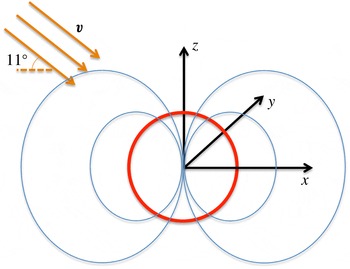
From the analytical expression (2.21), it is difficult to study the configuration of the magnetic field. For this purpose, we will plot the magnetic field lines induced by Earth in the presence of the solar wind. Our derivation for the magnetic potential (2.21) holds for any solar wind velocity orientation and assumes that the magnetic dipole moment has only a
 $z$
component. Thus, we choose a system with the configuration shown in figure 1. To generate the magnetosphere, we use the characteristic values for Earth, i.e. a magnetic dipole moment of
 $M=7.8\times 10^{22}~\text{A}~\text{m}^{-2}$
(Olson & Amit Reference Olson and Amit2006), solar wind speed values within the range
 $v=375{-}500~\text{km}~\text{s}^{-1}$
(Fisk & Sari Reference Fisk and Sari1973; Russell Reference Russell2000) and conductivities in the range
 ${\it\sigma}=10^{-7}{-}10^{-6}~\text{S}~\text{m}^{-1}$
(Fisk & Sari Reference Fisk and Sari1973; Sazhin Reference Sazhin1978). With these quantities, we obtain values for
 $k$
between
 $3.8\times 10^{-5}$
and
 $5\times 10^{-4}~\text{km}^{-1}$
. Since the magnetic dipole of Earth is tilted by
 ${\it\lambda}\simeq 11^{\circ }$
(Olson & Amit Reference Olson and Amit2006), we incorporate this tilt into the velocity vector, i.e.
 $\boldsymbol{v}=v(\cos ({\it\lambda}),0,-\sin ({\it\lambda}))$
, and its corresponding velocity potential
 ${\it\phi}_{v}$
, in order to keep the magnetic dipole oriented in the
 $z$
direction.
Diagram of our system for studying Earth’s magnetosphere. Here we show the orientation of the solar wind velocity
 $\boldsymbol{v}$
and the reference coordinate system
 $(x,y,z)$
. The red circle represents Earth and the loop-like blue lines represent the magnetic lines produced by a magnetic dipole.

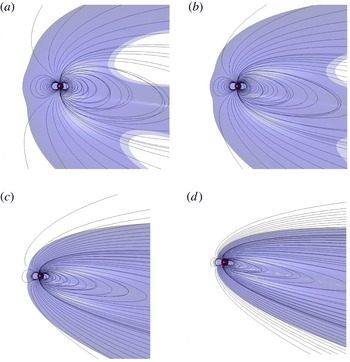
Terrestrial magnetic field deformed by the presence of the solar wind, which comes from left to right. We have varied the value of
 $k$
within the range of experimental observations, taking (a)
 $k=3.8\times 10^{-5}~\text{km}^{-1}$
, (b)
 $6.6\times 10^{-5}~\text{km}^{-1}$
, (c)
 $2\times 10^{-4}~\text{km}^{-1}$
and (d)
 $5\times 10^{-4}~\text{km}^{-1}$
. The red sphere represents Earth and the blue isosurface is located at
 ${\it\xi}\equiv |\boldsymbol{B}|/M=2.56~\text{nT}~\text{m}^{2}~\text{A}^{-1}$
.

In figure 2, we display the configuration of the magnetic lines. The blue isosurface is located at
 ${\it\xi}\equiv |\boldsymbol{B}|/M=2.56~\text{nT}~\text{m}^{2}~\text{A}^{-1}$
, which corresponds approximately to the magnitude of the magnetic field at the observed magnetopause (Sibeck, Lopez & Roelof Reference Sibeck, Lopez and Roelof1991). The magnetopause is a boundary layer that separates the magnetic field of a planet from the solar wind. It is usually determined by the balance between the magnetic pressure, which is approximately
 $|\boldsymbol{B}|^{2}/2{\it\mu}_{0}$
, and the dynamic pressure of the solar wind. In realistic magnetospheres, there is usually an abrupt change in the magnetic field at the magnetopause location. However, in our system, since we have not considered changes in the solar wind velocity, we can only estimate where the magnetic pressure should be large enough to introduce non-negligible deviations of the solar wind trajectory, by inspecting the isosurface at which the magnetic pressure coincides with that at the magnetopause in observational data (see figure 2). Note that as the value of
 $k$
is increased, the magnetic lines are deformed more strongly and the isosurface of constant magnetic field becomes narrower. However, for small values of
 $k$
, the shape qualitatively corresponds to the real terrestrial magnetosphere.
Given that the magnetopause is defined as the surface
 ${\it\xi}\equiv |\boldsymbol{B}|/M=2.56~\text{nT}~\text{m}^{2}~\text{A}^{-1}$
and there is an explicit formula (2.21) for the vector potential, one can compute
 $\boldsymbol{B}\equiv \boldsymbol{{\rm\nabla}}\times \boldsymbol{A}$
, find the characterisation of this surface in
 $(X,Y,Z)$
coordinates and then compute the average radius
 $R=\langle \sqrt{Y^{2}+Z^{2}}\rangle$
(with
 $\langle \cdots \rangle$
denoting spatial average) for each cross-section of the surface defined by a plane
 $X=\text{const}$
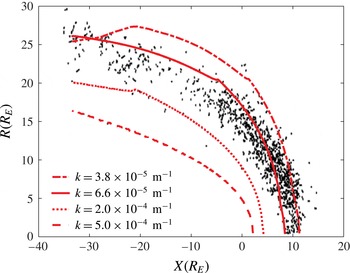
. By using this procedure, one can draw the shape of the magnetopause for various values of
 $k$
and make quantitative comparisons with observational data; see figure 3. In this figure, we observe good agreement between our predictions and the experimental observations. Note that as the value of
 $k$
is increased, the shape of the region deviates more from the experimental points; however, within a range of
 $k$
values our results are still in fair agreement. This is a satisfactory result, given that we do not a priori consider a magnetopause or solar wind deviations (due to the terrestrial magnetic field) in our model. It also confirms that the magnetopause can be described to a good approximation as a layer of constant magnetic pressure, since
 $|\boldsymbol{B}|^{2}/2{\it\mu}_{0}$
is also constant. Note that inside this region, where stronger magnetic fields are found, deviations of the solar wind cannot be neglected anymore.
Location and shape of the magnetopause. We have varied the value of
 $k$
within the range of experimental observations. The black points are experimental data (Sibeck et al.
Reference Sibeck, Lopez and Roelof1991), and the lines represent our theoretical results for
 ${\it\xi}=2.56~\text{nT}~\text{m}^{2}~\text{A}^{-1}$
. Here
 $R_{E}$
denotes the Earth radius and
 $R\equiv \langle \sqrt{Y^{2}+Z^{2}}\rangle$
, being the magnetopause located at
 $(X,Y,Z)$
, is the average radius measured for each cross-section of the surface by a plane
 $X=\text{const}$
.

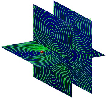
The Chapman–Ferraro currents are also reproduced at least qualitatively; see figure 4. The current density can be calculated from (2.21) by applying the curl operator twice,
 $\boldsymbol{J}=\boldsymbol{{\rm\nabla}}\times (\boldsymbol{{\rm\nabla}}\times \boldsymbol{A})/{\it\mu}$
. Here we see that the complex configuration of these currents is present even without considering deviations of the solar wind by the magnetic field. These currents are known to be responsible for the appearance of the magnetopause.
Induced electrical current density in the solar wind due to the presence of the terrestrial magnetic field. Here, the solar wind comes from left to right and
 $k=6.6\times 10^{-5}~\text{km}^{-1}$
. The green streamlines show the current density lines and the red sphere represents Earth. The electrical currents in the vertical planes are also known as Chapman–Ferraro currents.

4. Conclusions
In summary, we have found an analytical solution to the MHD equations for studying intrinsic magnetospheres. In order to obtain the solution, we introduced a new gauge condition so that analytical solution of the equations is possible. By substituting in actual values of the solar wind and terrestrial magnetic field, we find that our model is able to reproduce the shape of the actual magnetopause and also describe qualitatively the Chapman–Ferraro currents. Our results suggest that these features of the magnetosphere can be reproduced satisfactorily without having to take into account strong deviations of the solar wind by the terrestrial magnetic field; this also confirms that the magnetopause can be approximated by a layer of constant magnetic pressure. However, our model has several limitations; in particular, we assume a constant plasma velocity and neglect the effects of the magnetic field on the plasma. These assumptions limit the applicability of our model to understanding many interesting physical phenomena that occur in the magnetosphere; nevertheless, due to the model’s simplicity, it can be used to study the basic concepts concerning deformation of the terrestrial magnetosphere by the presence of solar wind.
The theoretical model proposed here can be applied to other kinds of planets by choosing different multipolar expansions of the solution to the MHD equations. Temporal perturbations and MHD instabilities can also be studied using our steady solution as the solution for the averaged fields and will be the subject of future research. Extensions to consider plasma deviations and formation of the magnetopause will also be considered in future work.
Acknowledgement
M.M. acknowledges financial support from the European Research Council (ERC) Advanced Grant 319968-FlowCCS.