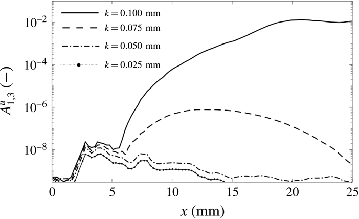
1 Introduction
Laminar–turbulent boundary-layer transition on blunt bodies is a critical issue in the design of hypersonic vehicles such as re-entry capsules. For fully turbulent boundary layers, the heat-transfer rate at the wall is significantly higher than in the laminar case. Uncertainties in transition prediction result in additional weight of the thermal protection system (TPS) and manufacturing costs aimed at guaranteeing the integrity of the vehicle. However, despite long-running investigations, transition on re-entry capsules still the defies full understanding. Already in the 1950s, experiments showed that early transition occurred on many spherical geometries, contrary to what was predicted by classical stability theory (Morkovin Reference Morkovin1984). In fact, the strongly favourable pressure gradient and the small values of the cross-flow velocity component typical of blunt bodies ensure that the boundary layer on smooth walls remains stable against both Tollmien–Schlichting (TS) waves and cross-flow instabilities even at very large Reynolds numbers. Furthermore, the presence of Görtler-type instabilities is prevented by the convex surface curvature. Transient growth has been suggested as a possible transition mechanism for blunt-body geometries by Reshotko & Tumin (Reference Reshotko, Tumin, Fasel and Saric2000, Reference Reshotko and Tumin2004) and the topic is still the subject of ongoing research (Paredes, Choudhari & Li Reference Paredes, Choudhari and Li2017; Hein et al.
Reference Hein, Theiss, Di Giovanni, Stemmer, Schilden, Schröder, Paredes, Choudhari, Li and Reshotko2018; Leidy et al.
Reference Leidy, Reshotko, Siddiqui and Bowersox2018). However, Hein et al. (Reference Hein, Theiss, Di Giovanni, Stemmer, Schilden, Schröder, Paredes, Choudhari, Li and Reshotko2018) showed that the
 $N$
-factors obtained through optimal transient-growth analysis on a blunt-capsule geometry are too small (
 $N\leqslant 3$
) to explain experimentally observed transition. In this context, wall roughness seems to be the most likely factor to influence blunt-body transition.
In the case of re-entry capsules, roughnesses are present on the thermal protection system as both localised non-uniformities and distributed roughness. Isolated roughness elements comprehend TPS joints, compression pads and gaps between heat-shield tiles, while the presence of distributed roughness is mainly associated with the ablation of the TPS. For laminar ablation, the roughness height is usually of the order of the boundary-layer thickness or smaller and larger roughness elements can apparently be generated only after transition occurs (Grabow & White Reference Grabow and White1974). Even though to date there is no general mechanism-based criterion to predict roughness-induced transition, the ratio of roughness height to boundary-layer thickness
 $k/\unicode[STIX]{x1D6FF}$
and the roughness Reynolds number
 $Re_{kk}=\unicode[STIX]{x1D70C}_{k}u_{k}k/\unicode[STIX]{x1D707}_{k}$
, defined with the flow properties at the roughness height for the corresponding smooth configuration, are regarded as the relevant parameters. A detailed review of experimental data on the effects of the roughness height and Reynolds numbers on transition location is presented by Schneider (Reference Schneider2008a
).
Initially, due to the complexity of the problem and to the lack of advanced computing resources, the phenomenon of roughness-induced transition on blunt bodies was studied experimentally. A review of available experimental data on the effects of roughness on hypersonic blunt-body transition is provided by Schneider (Reference Schneider2008b ).
The possible correlation between
 $Re_{kk}$
and transition on blunt geometries was investigated, among others, by Reda (Reference Reda2002). His analysis showed that three-dimensional, distributed roughness patterns promote earlier transition compared to single roughness elements with the same height and shape. In particular, in the case of distributed roughness elements, the critical
 $Re_{kk}$
can be 4–10 times smaller than the critical value of the corresponding case of isolated elements. Further analyses for blunt-body geometries with distributed sand-grain roughness were conducted by Reda et al. (Reference Reda, Wilder, Bogdanoff and Prabhu2008). The critical value for transition of
 $Re_{kk}$
, built with the arithmetic average of the measured roughness heights and fluid viscosity at the wall temperature, was found to be
 $250\pm 20\,\%$
in those investigations. Additional tests on blunt-body geometries were performed in a
 $\text{CO}_{2}$
and an air-dominated atmosphere by Wilder, Reda & Prabhu (Reference Wilder, Reda and Prabhu2015). The critical value for transition was
 $Re_{kk,tr}=259$
for tests conducted in air and
 $Re_{kk,tr}=223$
for tests conducted in
 $\text{CO}_{2}$
, with an uncertainty of
 $25\,\%$
.
Experimental measurements made at NASA Langley Research Center (LaRC) on scaled models of the Crew Exploration Vehicle (CEV) for Mach 6 and 10 are presented by Berger (Reference Berger2009). Laminar–turbulent transition was obtained with boundary-layer trips of
 $0.3$
–
 $0.8$
boundary-layer thicknesses in height. Further results from an experimental campaign conducted at LaRC for sphere–cone and hemisphere geometries with distributed roughness are summarised in Hollis (Reference Hollis2014). Sand-grain-type roughnesses as well as patterned roughnesses were considered. The free-stream Reynolds number was in the range of
 $Re_{\infty }=9.84{-}27.23\times 10^{6}~\text{m}^{-1}$
and the roughness Reynolds number
 $Re_{k^{+}}$
was defined with the friction velocity,
 $Re_{k^{+}}=\unicode[STIX]{x1D70C}_{w}u_{\unicode[STIX]{x1D70F}}k/\unicode[STIX]{x1D707}_{w}$
. Transitional flow was found for
 ${\sim}10<Re_{k^{+}}<\sim 70$
.
On the base of a blunt Apollo-like capsule at
 $M=5.9$
, numerical and experimental investigations have been conducted for wind-tunnel conditions at the Hypersonic Ludwieg Tube in Braunschweig (HLB) (Ali, Radespiel & Theiss Reference Ali, Radespiel and Theiss2014; Theiss et al.
Reference Theiss, Ali, Hein, Heitmann and Radespiel2014; Radespiel et al.
Reference Radespiel, Ali, Bowersox, Leidy, Tanno, Kirk and Reshotko2018). Using a standard infrared coating with a root-mean-square roughness of
 $\bar{k}\approx 10~\unicode[STIX]{x03BC}\text{m}$
, a surface-heating increase compared to the laminar case was observed for
 $Re_{\infty }\approx 18\times 10^{6}~\text{m}^{-1}$
. Experiments at the same Reynolds number for the highly polished surface did not show any evidence of transition. Numerical simulations and linear stability analyses for the equivalent smooth geometry revealed that the boundary layer is stable against TS-waves and cross-flow instabilities even at values of the Reynolds number much higher than the ones that could be investigated experimentally.
Numerically, the problem of roughness-induced transition has been investigated mainly for the case of isolated roughness elements, both at flat-plate and blunt configurations, whereas simulations of distributed roughnesses have mainly been performed on the basis of flat-plate geometries only. By means of direct numerical simulations (DNS), BiGlobal stability analysis and three-dimensional parallelised stability equations (PSE-3D), De Tullio et al. (Reference De Tullio, Paredes, Sandham and Theofilis2013) investigated the transition mechanisms behind a quadrilateral isolated roughness element on a flat plate at
 $M=2.5$
. For
 $Re_{kk}=170$
and
 $k/\unicode[STIX]{x1D6FF}=0.22$
, no acceleration of the laminar–turbulent transition process was observed. On the contrary, for
 $Re_{kk}=791$
and
 $k/\unicode[STIX]{x1D6FF}=0.44$
the roughness wake became very unstable. The two most dominant unstable modes have a symmetric (varicose) and an antisymmetric (sinuous) character, with the symmetric mode growing faster than the antisymmetric one. In the numerical investigations of Van den Eynde & Sandham (Reference Van den Eynde and Sandham2016), a variety of roughness shapes have been investigated on a flat plate at
 $M=6$
. The results highlighted that the growth of instabilities in the wake of the isolated roughness elements strongly depends on the shape of the roughness. In particular, an important factor is represented by the aft section of the roughness element and, hence, by the properties of the recirculation zone. The author suggested that the roughness profile is an important characteristic currently neglected in the commonly used engineering correlations. Further investigations on the influence of the roughness shape on the transition mechanisms have been presented by Groskopf & Kloker (Reference Groskopf and Kloker2016), who performed DNS to analyse the nonlinear disturbance evolution in a laminar, supersonic (
 $M=4.8$
) flat-plate boundary layer in the presence of a skewed roughness element. Similar dominant unstable modes were found as in the case of symmetric elements, with the shape of sinuous and varicose modes being tilted.
In the case of re-entry capsule geometries, Chang et al. (Reference Chang, Choudhari, Venkatachari and Li2011) performed numerical simulations on a CEV geometry at
 $M=6$
with both isolated surface protuberances and cavities. They showed that a protuberance with a
 $Re_{kk}=800$
and
 $k/\unicode[STIX]{x1D6FF}=0.73$
produces a strong wake instability and spontaneous vortex shedding and the flow is more unstable than in the case of a cavity of identical geometry. For the case of a generic three-dimensional (3-D) Apollo-capsule geometry with an angle of attack, Theiss et al. (Reference Theiss, Hein, Ali and Radespiel2016, Reference Theiss, Leyh and Hein2017) investigated the modal instability mechanisms of the steady wake developing downstream of isolated roughness elements positioned on the windward side of the capsule. Computation of the laminar, steady base flow was conducted at the
 $M=5.9$
free-stream conditions of the HLB and values of
 $Re_{kk}$
in the range of 124–336 were considered. Stability analyses were conducted with the help of two-dimensional linear stability theory (LST-2D) and PSE-3D. It was found that the most unstable modes have the same symmetric and antisymmetric features as the modes found in the wake of isolated roughness elements in the case of the flat plate. An
 $N$
-factor of almost
 $8$
was found for the case of symmetric mode for a cylindrical roughness element with
 $Re_{kk}=336$
.
With regard to surfaces with distributed roughness, some numerical investigations have been performed in the case of a flat plate. Brehm et al. (Reference Brehm, Dackermann, Grygier and Fasel2011) analysed the effects of two-dimensional, sinusoidal and rectangular roughness elements on the stability of the incompressible boundary layer. They found that the growth of small disturbances is larger for sinusoidal roughness elements than for rectangular ones. It was suggested that the increased amplification might be related to the extended region of separated flow induced by the sinusoidal shape. Furthermore, the effects of pressure gradient on the disturbance growth in the case of a rough wall seems to be less pronounced than in the case of a smooth wall. The three-dimensional case of distributed, sinusoidal roughness elements on a flat plate was numerically investigated by Muppidi & Mahesh (Reference Muppidi and Mahesh2012) for a supersonic boundary layer (
 $M=2.9$
). In this case, paired streamwise vortices resulted from an upward impulse provided by the roughness surface to the near-wall fluid.
Steady numerical simulations of the Blasius incompressible boundary layer altered by randomly distributed roughness were conducted by Drews et al. (Reference Drews, Downs, Doolittle, Goldstein and White2011). In this case, the main vorticity cores in the roughness wake are associated with the highest peaks of the roughness patch. Both counter-rotating vortex pairs and single vortex cores are generated according to the shape of the roughness and its alignment with the free stream. The steady base flow in the wake of the roughness patch was compared with the corresponding experimental results (Downs, White & Denissen Reference Downs, White and Denissen2008). Steady numerical simulations were undertaken by Di Giovanni & Stemmer (Reference Di Giovanni, Stemmer and Dillmann2017) to investigate the boundary layer of a 3-D capsule geometry with a patch of randomly distributed roughness under re-entry conditions (
 $M=20$
). The analysis mainly focused on the development and interaction of the steady high-vorticity regions in the roughness wake and on the influence of chemical reactions and non-equilibrium effects.
In this work we study the instability modes, in both the linear and nonlinear stages until laminar breakdown, developing in the boundary layer of a hemisphere geometry with a rough wall. The growth of unsteady disturbances forced in the inflow is analysed and quantified with DNS. Two different roughness geometries are considered: an array of spanwise periodic roughness elements and a more realistic random distributed roughness. Here, the term random is used to indicate the superposition of different sinusoidal waves with pseudo-random amplitudes and phases. In the present work, the prefix ‘pseudo-’ will be omitted for brevity for the remaining part of the paper. Free-stream conditions have been chosen to match the wind-tunnel conditions at HLB at
 $M=5.9$
.
In § 2 the considered geometries as well as the numerical set-up are presented. The methods of the analysis are illustrated in § 2.5. In § 3 the flow in the case of spanwise periodic roughness elements is studied. Features of the base flow and stability properties of the main instability modes in the wake of the roughness are presented and compared. Results from linear stability analysis and from PSE analysis are also shown for cross-validation. In § 4 the flow in the presence of randomly distributed roughness is investigated. The development of disturbance modes is described and quantified in the linear and nonlinear stages of the transition process. A discussion of the comparison between the two roughness geometries is also included. Summary and conclusions are presented in § 5.
2 Configurations and numerical set-up
2.1 DNS-solver
Parallel DNS are conducted with the semi-commercial solver Navier–Stokes Multi Block (NSMB). The NSMB code is documented in Vos, Duquesne & Lee (Reference Vos, Duquesne and Lee1999) and Hoarau et al. (Reference Hoarau, Pena, Vos, Charbonier, Gehri, Braza, Deloze and Laurendeau2016) and it has been successfully applied in numerous studies of hypersonic flows (von Kaenel et al. Reference von Kaenel, Sanchi, Vos, Gaffuri, Leyland, Walloschek and Binetti2009; Goebel, Vos & Mundt Reference Goebel, Vos and Mundt2012; Stemmer & Fehn Reference Stemmer and Fehn2014; Di Giovanni & Stemmer Reference Di Giovanni, Stemmer and Dillmann2017; Stemmer, Birrer & Adams Reference Stemmer, Birrer and Adams2017a ,Reference Stemmer, Birrer and Adams b ; Hein et al. Reference Hein, Theiss, Di Giovanni, Stemmer, Schilden, Schröder, Paredes, Choudhari, Li and Reshotko2018). The code is finite-volume based and it works with structured grids divided in multiple blocks using the message-passing interface (MPI) environment.
A variety of numerical schemes can be used. In the presence of a bow shock in the computational domain, steady simulations are performed starting with an advection upstream splitting method (AUSM
 $+$
) upwind scheme of first-order accuracy and an implicit Euler time integration based on a lower–upper symmetric Gauss–Seidel method. Once the shock has been established, better accuracy of the solution is reached by continuing the computation with a central discretisation scheme of second-order accuracy and an explicit five-stage Runge–Kutta time-integration scheme. The shock is captured with a shock fitting mesh and explicit second- and fourth-order artificial-dissipation terms are locally added to the numerical scheme to suppress spurious oscillations. In the computational domain without bow shock, DNS are performed with a more accurate central discretisation scheme of fourth-order accuracy and a five-stage Runge–Kutta time-integration scheme.
2.2 Computational domain and boundary conditions
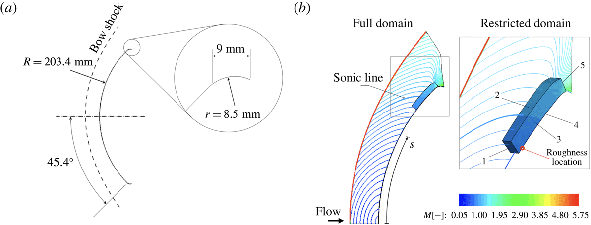
Details of geometry and size of the hemisphere are given in figure 1. The hemisphere has an angular extension of approximately
 $90^{\circ }$
and it ends in a shoulder closely resembling that of a generic Apollo capsule geometry. The shoulder acts as a natural damping region through the strong flow acceleration and prevents undesired reflection of unsteady disturbances at the numerical outflow boundary.
The flow over the considered hemisphere geometry has already been shown to be almost identical to the flow over the Apollo capsule model at an angle of attack of
 $24^{\circ }$
used in the experiments at HLB (Hein et al.
Reference Hein, Theiss, Di Giovanni, Stemmer, Schilden, Schröder, Paredes, Choudhari, Li and Reshotko2018). In comparison to the capsule geometry with an angle of attack, the hemisphere geometry allows for a significant reduction of the computational domain and effort due to azimuthal periodicity of the domain. In the experiments at HLB, a Plexiglas capsule model with a Nextel Velvet coating was used for optical measurements of the surface temperature. The coating was sanded to provide a distributed roughness with a root-mean-square value of
 $\bar{k}=10~\unicode[STIX]{x03BC}\text{m}$
. As the simulation of the entire rough-wall capsule would have been extremely expensive, only a small roughness patch on the hemisphere’s wall is considered in the present work. Besides, as the boundary layer observed in the experiments at HLB was never fully turbulent for the investigated roughness, a larger roughness height corresponding to a mean roughness of
 $\bar{k}\approx 22~\unicode[STIX]{x03BC}\text{m}$
is used in the present numerical simulations (for more details of the roughness geometry see § 2.3).
(a) Scheme of the investigated hemisphere geometry. (b) Full and restricted domains with the Mach number colour coded.

To ease the computational effort in the case of unsteady simulations on the rough-wall configuration, a two-stage simulation is performed on two different simulation domains, as shown in figure 1. In the first simulation step, the flow over the entire hemisphere (full domain) is considered. This domain extends from the stagnation point to the shoulder and includes the bow shock ahead of the blunt body. The steady base flow is computed on a smooth-wall, two-dimensional, axisymmetric grid consisting of approximately 76 000 points clustered around the shock location and inside the boundary layer (figure 2). Previous simulations with the same grid resolution have been successfully compared with experimental results as well as with results from other numerical simulations including a grid study (Stemmer & Fehn Reference Stemmer and Fehn2014; Di Giovanni & Stemmer Reference Di Giovanni, Stemmer and Dillmann2017). For free-stream and far-field boundaries, characteristic variables are used. The wall is modelled as isothermal with a constant temperature of
 $T_{w}=295~\text{K}$
, as measured in the corresponding experiments. Free-stream conditions match the wind-tunnel conditions at HLB and are listed in table 1. In particular, with a free-stream temperature of
 $59~\text{K}$
, the air temperature after the bow shock does not exceed
 $500~\text{K}$
and the model of a calorically and thermally perfect gas can be applied in the simulations.
Computational grid of the full domain (every second point shown) and close-up of the computational grid of the restricted domain (every sixth point shown).

Free-stream conditions for the present simulations.

The results for the full domain are used to generate the boundary conditions for a second restricted domain. Since the shock is excluded from the restricted domain, a fourth-order central discretisation scheme is used. Moreover, the grid resolution is increased to resolve the boundary layer in the presence of the rough wall. A grid-convergence study for the restricted domain is presented in § 2.3.
The curvilinear coordinate
 $s$
has its origin set on the stagnation point and it extends parallel to the wall until the end of the shoulder. With reference to
 $s$
, the restricted domain is extracted for
 $s\in [125.3,164.0]~\text{mm}$
. In this region, the boundary layer is transonic to supersonic.
Computations are performed on a Cartesian coordinate system. For clarity purposes, results hereafter are represented on a spherical coordinate system, with
 $x$
,
 $y$
and
 $z$
being the streamwise, wall-normal and spanwise direction, respectively. In particular,
 $x=0$
is set to
 $s=125.3~\text{mm}$
and the domain is centred on the plane
 $z=0$
. In the spherical part of the domain, excluding the shoulder, the coordinates
 $x$
,
 $y$
and
 $z$
are given by
 $$\begin{eqnarray}\left.\begin{array}{@{}c@{}}\displaystyle x=R\unicode[STIX]{x1D703}_{1}-0.1253,\\ \displaystyle y=r-R,\\ \displaystyle z=R\unicode[STIX]{x1D703}_{2}\sin \unicode[STIX]{x1D703}_{1},\end{array}\right\}\end{eqnarray}$$
where
 $r$
is the distance from the centre of the hemisphere,
 $\unicode[STIX]{x1D703}_{1}$
the elevation angle with reference to the stagnation point and
 $\unicode[STIX]{x1D703}_{2}$
the azimuth angle measured clockwise on the rotation axis of the two-dimensional domain. With reference to this coordinate system, the extension of the restricted domain in the wall-normal direction is approximately
 $y=7~\text{mm}$
, corresponding to almost 20 boundary-layer thicknesses at the roughness location. The angular extension of the restricted domain in the spanwise direction depends on the considered roughness geometry and is discussed in more detail in § 2.3. Dirichlet boundary conditions are applied at the inflow boundaries (faces 1 and 2 in figure 1), azimuthal–periodic boundary conditions are used in the spanwise direction (face 3) and Riemann invariants are used at the outflow (face 5). Finally, face 4 is the no-slip isothermal wall.
2.3 Characterisation of the roughness patch and grid studies
Two different types of roughness geometries are investigated. First, we consider an array of spanwise periodic roughness elements, where the projection of the roughness profile in the
 $y$
–
 $z$
plane is a simple sine function. Second, a more realistic randomly distributed roughness is considered. The patch of distributed roughness is obtained from the superposition of different sinusoidal functions with different wavelengths and random amplitudes and phases. In both cases, the roughness patch is modelled using a body-fitted grid. Body-fitted grids have been successfully applied to model roughness elements in the works of Muppidi & Mahesh (Reference Muppidi and Mahesh2012), Groskopf & Kloker (Reference Groskopf and Kloker2016) and Van den Eynde & Sandham (Reference Van den Eynde and Sandham2016). A detailed description of each roughness geometry and corresponding grid is given hereafter. The location of the roughness patch on the capsule was chosen at a position where the local boundary-layer edge velocity is sufficiently large to provide values of the roughness Reynolds number in the range of 400 for roughness heights significantly smaller than the boundary-layer thickness.
2.3.1 Spanwise periodic roughness elements
The computational grid at the roughness surface for the roughness type with spanwise periodic elements is shown in figure 3. The roughness patch starts at
 $x=7.75~\text{mm}$
. As the domain is represented in a spherical coordinate system, the value of the wavelength
 $\unicode[STIX]{x1D706}_{0}$
is expressed in terms of the elevation angle
 $\unicode[STIX]{x1D703}_{1}$
and is given by
 $$\begin{eqnarray}\unicode[STIX]{x1D706}_{0}=\frac{2\unicode[STIX]{x03C0}}{N_{\unicode[STIX]{x1D703}}}R\sin \unicode[STIX]{x1D703}_{1},\end{eqnarray}$$
with
 $N_{\unicode[STIX]{x1D703}}$
an integer number. In order to detect the presence of possible subharmonic modes in the analysis of the unsteady flow, the computational domain in the spanwise direction contains two times the wavelength
 $\unicode[STIX]{x1D706}_{0}$
, i.e. the spanwise extension of the domain is
 $(4\unicode[STIX]{x03C0}/N_{\unicode[STIX]{x1D703}})R\sin \unicode[STIX]{x1D703}_{1}$
.
The spanwise extension of the roughness is
 $\unicode[STIX]{x1D706}_{0,r}$
, where the subscript
 $r$
indicates the value taken at the elevation corresponding to the roughness position. In the streamwise direction, the length of the roughness patch is
 $\unicode[STIX]{x1D706}_{0,r}/2$
. The surface height with respect to the smooth configuration is given by
 $$\begin{eqnarray}h(x,z)=kg_{1}(x)\cos \left(\frac{2\unicode[STIX]{x03C0}}{\unicode[STIX]{x1D706}_{0}}(x+z)\right),\end{eqnarray}$$
where
 $k$
is the roughness height and
 $g_{1}(x)$
a piecewise defined function which ensures continuity with the smooth wall. In particular,
 $g_{1}(x)$
consists of two fifth-order polynomials in the range from zero to
 $1$
within a length of
 $\unicode[STIX]{x0394}x=\unicode[STIX]{x1D706}_{0,r}/4$
, yielding a continuous and smooth flattening of the roughness boundaries, and is zero outside the roughness patch. The roughness height is
 $k=0.1~\text{mm}$
. The roughness height is the same as that of the isolated roughness elements investigated in Theiss et al. (Reference Theiss, Hein, Ali and Radespiel2016).
Envelope function
 $g_{1}(x)$
(a) and grid close to the array of spanwise periodic roughness elements (b). For clarity, only every second point is shown.

In the case of spanwise periodic roughness elements, the roughness patch is centred at
 $\unicode[STIX]{x1D703}_{0,r}=37.6^{\circ }$
and
 $N_{\unicode[STIX]{x1D703}}=650$
, which yields
 $\unicode[STIX]{x1D706}_{0,r}=1.2~\text{mm}$
. This value is of the same order of magnitude as the boundary-layer thickness. The values chosen for
 $k$
and
 $\unicode[STIX]{x1D706}_{0,r}$
guarantee a low skewness for all grid cells at the wall, while also providing a roughness profile in good approximation resembling a realistic sand-grain roughened wall (see e.g. Hollis Reference Hollis2017). The ratio of the roughness height to the boundary-layer thickness is
 $k/\unicode[STIX]{x1D6FF}=0.35$
and the roughness Reynolds number is
 $Re_{kk}=421$
. For these values of the roughness variables, modal growth in the roughness wake is expected. Values of further roughness-related variables are listed in table 2 for both grid geometries analysed in this work. These variables are the mean roughness height
 $\bar{k}$
computed as the root-mean-square with reference to
 $y=0$
over the roughness patch, the mean roughness height to boundary-layer thickness ratio
 $\bar{k}/\unicode[STIX]{x1D6FF}$
, the roughness Reynolds number
 $Re_{k}=\unicode[STIX]{x1D70C}(k)u(k)k/\unicode[STIX]{x1D707}_{w}$
using the density and velocity at
 $y=k$
and the viscosity at wall temperature and the roughness Reynolds number
 $Re_{\bar{k}\bar{k}}=\unicode[STIX]{x1D70C}(\bar{k})u(\bar{k})\bar{k}/\unicode[STIX]{x1D707}(\bar{k})$
using flow properties at
 $y=\bar{k}$
. The boundary-layer thickness
 $\unicode[STIX]{x1D6FF}$
is the wall-normal distance where the flow reaches
 $99\,\%$
of the total free-stream enthalpy.
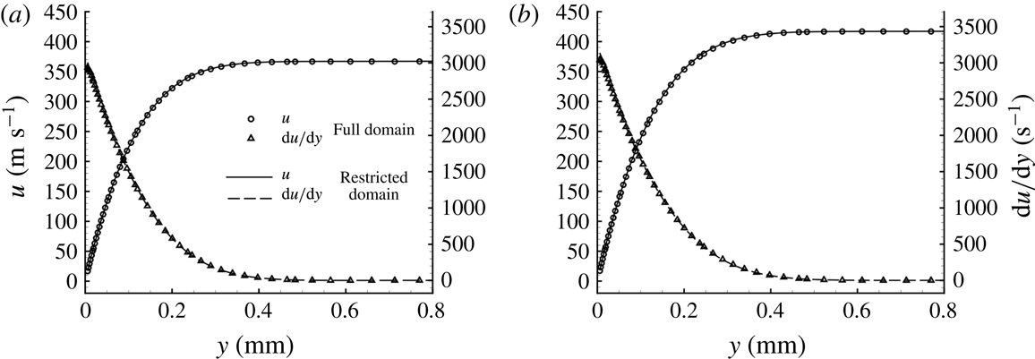
Profiles of the velocity and derivative of the velocity in the wall-normal direction at
 $x=10~\text{mm}$
(a) and
 $x=30~\text{mm}$
(b).

Roughness variables for the two roughness types investigated in this work.

2.3.2 Size of the computational domain and grid convergence
Careful analysis of the solutions in the full domain and in the restricted domain has been carried out to check the absence of errors which may rise because of the different computational schemes and grid resolutions used in the two different domains. The boundary-layer profiles on the full and restricted domains have been compared for the smooth-wall configuration at different positions. Profiles of the velocity and derivative of the velocity in the wall-normal direction are shown in figure 4 for
 $x=10~\text{mm}$
and
 $x=30~\text{mm}$
. No appreciable differences are present between the results for the two domains. Therefore, a negligible error is made when passing from the full domain to the restricted domain. The accuracy of the steady simulations as well as the absence of numerically produced unsteady disturbances are further guaranteed by achieving very good convergence of the residuals.
Particular attention has been paid to ensuring that the presence of the roughness patch does not induce disturbances outside the boundary layer, influencing the results through interaction with the upper boundary or the inflow boundary of the integration domain. The roughness height is significantly smaller than the boundary-layer thickness and the Mach number at the roughness height in the smooth-wall configuration is 0.6. In the wall-normal direction, the computational domain extends to almost
 $y=7~\text{mm}$
, corresponding to almost 20 boundary-layer thicknesses.
Due to the strong acceleration of the flow, the boundary layer grows slowly and the boundary-layer thickness increases by approximately
 $14\,\%$
between
 $x=0~\text{mm}$
and
 $x=30~\text{mm}$
. Note that the ratio of the domain height to boundary-layer thickness in the present work is larger than the values found in other numerical works on roughness-induced transition of high-speed boundary layers with comparable roughness features, such as in De Tullio et al. (Reference De Tullio, Paredes, Sandham and Theofilis2013), Groskopf & Kloker (Reference Groskopf and Kloker2016) and Muppidi & Mahesh (Reference Muppidi and Mahesh2012). Further extension of the domain size did not result in any noticeable variation of the flow solution. In addition, the height of the upper boundary (face 2) guarantees that, for the unsteady simulations, any potential residual reflections at the upper boundary exit the domain at the outflow boundary without impinging on the boundary layer and, hence, without affecting the stability properties of the roughness wake.
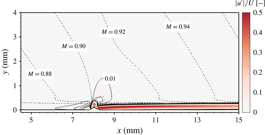
Absolute values of the roughness-induced steady disturbances of velocity (colour coded) and Mach number (dashed lines). The disturbances are normalised with the boundary-layer edge velocity and five isolines between 0.01 and 0.05 are represented with solid lines.

The effect of the roughness on the steady base flow is limited to the viscous boundary-layer region downstream of the roughness location. This aspect is evidenced in figure 5, which shows the steady disturbances of the velocity obtained as absolute value of the difference between smooth-wall and rough-wall simulations. The values are normalised with the boundary-layer edge values of the streamwise velocity and isolines of the disturbance corresponding to
 $1\,\%$
of the edge values are labelled with 0.01. Isolines of the Mach number are also shown. Values are shown for the
 $z$
-plane intersecting the roughness peak where the maximum disturbance is found. For clarity purposes, the restricted domain is represented up to
 $y=4~\text{mm}$
only. The effects of the roughness remain limited to the boundary-layer region and do not induce any inviscid effects outside the boundary layer.
A grid-convergence study has been conducted with the numerical grids listed in table 3. The different grids are identified by
 $G_{i}$
, where the index
 $i$
is the grid number.
 $N_{x}$
,
 $N_{y}$
and
 $N_{z}$
are the number of points in the streamwise, wall-normal and spanwise directions, respectively, while
 $N_{tot}$
is the total number of grid points,
 $n_{y}^{\unicode[STIX]{x1D6FF}}$
is the number of points in the wall-normal direction inside the boundary layer and
 $n_{z}^{\unicode[STIX]{x1D706}}$
the number of points used to resolve one roughness wavelength in the spanwise direction.
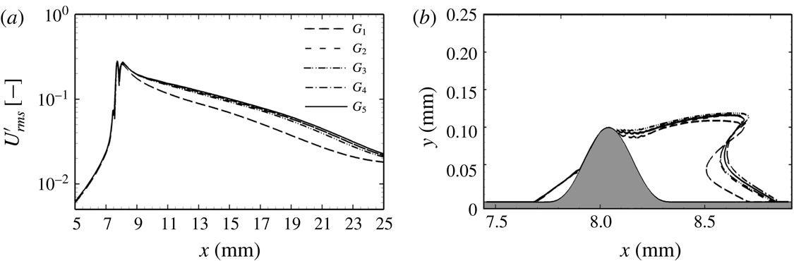
The relevant parameter in the grid-convergence study is the amplitude of the root-mean-square of the disturbance velocity,
 $$\begin{eqnarray}U_{rms}^{\prime }=\max _{y}\left(\frac{1}{\unicode[STIX]{x1D706}_{0}}\int _{0}^{\unicode[STIX]{x1D706}_{0}}u(x,y,z)-u_{b}(x,y,z)\,\text{d}z\right),\end{eqnarray}$$
where
 $u(x,y,z)$
is the streamwise velocity in the case of a rough wall and
 $u_{b}(x,y,z)$
is the streamwise velocity for the smooth configuration. The values of
 $U_{rms}^{\prime }$
over
 $x$
are shown in figure 6(a) normalised with the boundary-edge velocity at the roughness position.
A grid with a medium resolution (
 $G_{2}$
) already provides good results. By further increasing the number of grid points in both the
 $x$
- and
 $y$
-direction (
 $G_{3}$
) or in the
 $z$
-direction (
 $G_{4}$
and
 $G_{5}$
), no significant improvement of the solution is observed. For completeness, figure 6(b) shows the recirculation zone downstream of the roughness for different grid resolutions. We found that
 $80$
grid points per wavelength
 $\unicode[STIX]{x1D706}_{0}$
are sufficient (
 $G_{4}$
). Simulations for the case of spanwise periodic roughness elements are performed on the grid
 $G_{5}$
, which corresponds to a medium resolution in the
 $x$
- and
 $y$
-direction and a fine resolution in the
 $z$
-direction.
Results of the grid-convergence analysis:
 $U_{rms}^{\prime }$
along
 $x$
(a) and recirculation zone as the zero-velocity line at
 $z=0$
(b).

Computational grids used in the grid-convergence study.

2.3.3 Randomly distributed roughness
The computational grid at the roughness surface for the randomly distributed roughness type is shown in figure 7. The patch shape is obtained by superposing different sinusoidal waves with pseudo-random amplitudes and phases. According to the definition of distributed roughness also presented in Downs et al. (Reference Downs, White and Denissen2008), the surface height with respect to the smooth configuration is given by
 $$\begin{eqnarray}h(x,z)=kg_{2}(x)\mathop{\sum }_{m,n=1}^{5}A_{m,n}\cos \left(\frac{2\unicode[STIX]{x03C0}m}{5\unicode[STIX]{x1D706}_{0}}x+\frac{2\unicode[STIX]{x03C0}n}{5\unicode[STIX]{x1D706}_{0}}z+\unicode[STIX]{x1D719}_{m,n}\right),\end{eqnarray}$$
with
 $\unicode[STIX]{x1D719}_{m,n}\in [0,2\unicode[STIX]{x03C0}]$
. Values of
 $A_{m,n}$
and
 $\unicode[STIX]{x1D719}_{m,n}$
have been randomly extracted from a uniform distribution and are listed in table 4. Values of
 $A_{m,n}$
are normalised with the maximum of the absolute value of the summation term in (2.5). Therefore, the maximum height of the roughness is
 $k$
and equal to
 $0.1~\text{mm}$
, as in the case of spanwise periodic roughness elements. The largest roughness wavelength is equal to five times
 $\unicode[STIX]{x1D706}_{0,r}$
. Values of
 $A_{m,n}$
with
 $n^{2}+m^{2}>5^{2}+1$
are set to zero in order to ensure a minimum roughness wavelength of
 $\unicode[STIX]{x1D706}_{0,r}$
in all directions.
The roughness patch starts at
 $x=2.5~\text{mm}$
and its length in the
 $x$
-direction is
 $5\unicode[STIX]{x1D706}_{0,r}$
. As shown by the analysis in § 3.2, subharmonic modes are found to be negligible in this set-up. Hence, in order to limit the size of the simulation, the angular extension of the domain in the spanwise direction is
 $(2\unicode[STIX]{x03C0}/130)R\sin \unicode[STIX]{x1D703}_{1}$
and is designed to contain the fundamental wavelength
 $5\unicode[STIX]{x1D706}_{0}$
.
Envelope function
 $g_{2}(x)$
(a) and computational grid close to the randomly distributed roughness patch (b). For clarity, only every fifth point is shown.

The highest peak in the distributed roughness is found at
 $x_{k}=4.80~\text{mm}$
. Since this position does not correspond to that of the roughness peak in the case of spanwise periodic roughness elements, a slightly different roughness Reynolds number is found (
 $Re_{kk}=406$
). Nevertheless, as the boundary layer grows very slowly, the ratio of roughness height to boundary-layer thickness remains nearly unchanged and is equal to
 $h/\unicode[STIX]{x1D6FF}=0.35$
.
Amplitude coefficients (left) and phases (right) used in (2.5).

The smallest wavelength in the roughness patch is
 $\unicode[STIX]{x1D706}_{0,r}$
and, as shown in the case of spanwise periodic roughness elements, a resolution of
 $80$
grid points per
 $\unicode[STIX]{x1D706}_{0}$
provides good grid-convergence properties. Therefore, a grid with the same resolution properties as grid
 $G_{4}$
in table 3 is chosen. The grid for the randomly distributed roughness patch consists of
 $1120$
grid points in the streamwise direction,
 $160$
in the wall-normal direction and
 $400$
in the spanwise direction.
2.4 Disturbance generation
The boundary layer for the smooth-wall configuration is stable against modal growth throughout the entire domain. Thus, profiles of the disturbance for the unsteady simulations could not be deduced by linear stability theory. Only pressure disturbances are introduced at the inflow of the restricted domain (face 1). In a short region downstream of the inflow boundary upstream of the roughness patch, velocity disturbances generated by the pressure disturbances appear at a very low amplitude and are attenuated exponentially. The variation of this region moving the location of the inflow boundary further upstream with the fixed roughness location had no effect on the results as shown.
The disturbance is a zero-mean, time-varying function characterised by a single frequency
 $f_{1}$
,
 $$\begin{eqnarray}p^{\prime }(y,z,t)=c(y)\hat{p}_{0}(z)\sin (2\unicode[STIX]{x03C0}f_{1}t),\end{eqnarray}$$
where the function
 $c(y)=\text{e}^{-(y/\unicode[STIX]{x1D6FF})^{3}}$
guarantees that the perturbation vanishes outside the boundary layer and
 $\hat{p}_{0}(z)$
describes the amplitude of the pressure disturbance at the inflow. For the analysis of symmetric instability modes,
 $\hat{p}_{0}(z)$
is a constant value (i.e.
 $\hat{p}_{0}(z)=P_{0}$
) and the disturbance is a two-dimensional wave constant in the spanwise direction. For the analysis of antisymmetric instability modes,
 $\hat{p}_{0}(z)$
is a sine function odd with respect to
 $z=0$
given by
 $\hat{p}_{0}(z)=P_{0}\sin (2\unicode[STIX]{x03C0}z/\unicode[STIX]{x1D706}_{0})$
, with
 $\unicode[STIX]{x1D706}_{0}$
the spanwise period of the roughness patch. The unsteady inflow condition
 $p(0,y,z,t)$
is obtained by adding the function
 $p^{\prime }(y,z,t)$
to the value of the pressure prescribed at the boundary for the steady flow,
 $$\begin{eqnarray}p(0,y,z,t)=p_{0}(0,y,z)+p^{\prime }(y,z,t).\end{eqnarray}$$
In order to study linear growth of the introduced unsteady disturbances, the constant
 $P_{0}$
is kept several orders of magnitude smaller than the value of the boundary-layer pressure at the inflow position. In particular, the ratio of the inflow disturbance and the inflow value of the steady flow is
 $P_{0}/p_{0}(0,0,z)\approx 6\times 10^{-6}$
.
A single disturbance frequency equal to
 $250~\text{kHz}$
is investigated. This value has been chosen based on numerical LST-2D investigations of the base flow with a rough wall. The value of the disturbance frequency falls into the range of relevant frequencies measured in the experiments with transitional flow conducted at HLB for the rough-wall capsule geometry (Theiss et al.
Reference Theiss, Ali, Hein, Heitmann and Radespiel2014, Reference Theiss, Hein, Ali and Radespiel2016).
2.5 Stability analyses
2.5.1 LST-2D and PSE-3D analyses
The flow variable
 $q$
is split into a steady primary state
 $\bar{q}$
and an unsteady perturbation part
 $\tilde{q}$
. The LST-2D analysis is based on the assumption of a locally parallel base flow, i.e.
 $\bar{q}$
is assumed to be two-dimensional with the velocity component normal to the wall assumed to be zero. Streamwise gradients of the base flow are neglected. The unsteady perturbation
 $\tilde{q}$
is three-dimensional and periodic in
 $x$
at each instant in time. The spatial framework is used, with real frequency
 $\unicode[STIX]{x1D714}$
and complex wavenumber
 $\unicode[STIX]{x1D6FC}$
. The real part of
 $\unicode[STIX]{x1D6FC}$
defines the wavenumber of
 $\tilde{q}$
in the
 $x$
-direction, whereas the imaginary part defines the growth rate,
 $\unicode[STIX]{x1D70E}=-\text{Im}(\unicode[STIX]{x1D6FC})$
.
The linear PSE-3D solver is formulated in primitive variables and is based on the non-dimensional Navier–Stokes equations. The steady primary state
 $\bar{q}$
and the unsteady perturbation part
 $\tilde{q}$
are assumed to be three-dimensional and slowly varying in the streamwise direction. The disturbance growth of the wake modes is measured in terms of the total disturbance kinetic energy
 $E$
,
 $$\begin{eqnarray}E=\int _{-\infty }^{-\infty }\int _{-\infty }^{-\infty }|\bar{\unicode[STIX]{x1D70C}}|(|\hat{u} |^{2}+|\hat{v}|^{2}+|{\hat{w}}|^{2})\,\text{d}y\,\text{d}z,\end{eqnarray}$$
with
 $|\hat{u} |$
,
 $|\hat{v}|$
and
 $|{\hat{w}}|$
the amplitude of the velocity disturbances. The growth rate is defined by
 $$\begin{eqnarray}\unicode[STIX]{x1D70E}=-\text{Im}(\unicode[STIX]{x1D6FC})+\frac{\unicode[STIX]{x2202}}{\unicode[STIX]{x2202}x}\text{ln}(\sqrt{E}).\end{eqnarray}$$
The full description and verification of both PSE-3D and LST-2D solvers are presented in the work of Theiss et al. (Reference Theiss, Hein, Ali and Radespiel2016). PSE-3D as well as LST-2D analyses are used here for comparison and cross-validation only.
2.5.2 Two-dimensional Fourier analysis of the unsteady disturbances
Spatio-temporal analysis of the DNS is performed by means of two-dimensional fast Fourier transform. The generic flow variable
 $q(x,y,z,t)$
is decomposed into a spanwise wavenumber–frequency spectrum,
 $$\begin{eqnarray}Q_{m,n}(x,y)=\mathop{\sum }_{j=0}^{J-1}\mathop{\sum }_{l=0}^{L-1}q(x,y,z_{j},t_{l})\text{e}^{-\text{i}2\unicode[STIX]{x03C0}\left(nj/J+ml/L\right)},\end{eqnarray}$$
where
 $L$
and
 $J$
are the number of time and space samples, respectively. The spatio-temporal modes are indicated by (
 $m,n$
), where
 $m$
identifies multiples of the fundamental frequency and
 $n$
multiples of the fundamental spanwise wavenumber. In particular, (
 $1,1$
) is a three-dimensional wave with frequency
 $f_{1}$
and wavelength equal to the spanwise extension of the computational domain. The amplitude of the mode (
 $m,n$
) for the variable
 $q$
is defined at each position
 $x$
as the local maximum in the wall-normal direction:
 $$\begin{eqnarray}A_{m,n}^{q}(x)=\max _{y\geqslant 0}|Q_{m,n}(x,y)|.\end{eqnarray}$$
In addition, the growth rate of the disturbance associated with each frequency is computed with reference to the disturbance energy as in De Tullio et al. (Reference De Tullio, Paredes, Sandham and Theofilis2013). Mack’s disturbance energy norm (Mack Reference Mack1969) is expressed as
 $$\begin{eqnarray}{\mathcal{E}}_{m}(x)=\int _{0}^{\unicode[STIX]{x1D6FF}}\hat{\unicode[STIX]{x1D70C}}_{0}[\hat{U} _{m}^{2}+\hat{V}_{m}^{2}+{\hat{W}}_{m}^{2}]+\frac{\hat{\unicode[STIX]{x1D70C}}_{m}^{2}\hat{T}_{0}}{\unicode[STIX]{x1D6FE}\hat{\unicode[STIX]{x1D70C}}_{0}M^{2}}+\frac{\hat{T}_{m}^{2}\hat{\unicode[STIX]{x1D70C}}_{0}}{\unicode[STIX]{x1D6FE}(\unicode[STIX]{x1D6FE}-1)\hat{T}_{0}M^{2}}\,\text{d}y,\end{eqnarray}$$
with the disturbance amplitude associated with each frequency computed as
 $$\begin{eqnarray}\hat{Q}_{m}(x,y)=\mathop{\sum }_{n=0}^{N}|Q_{m,n}(x,y)|.\end{eqnarray}$$
The growth rate is computed as
 $$\begin{eqnarray}\unicode[STIX]{x1D70E}_{{\mathcal{E}}}=\frac{1}{2}\frac{\text{d}}{\text{d}x}\ln ({\mathcal{E}}_{m}(x)).\end{eqnarray}$$
In the investigated domain, the terms relative to the inner energy in the definition of the disturbance energy norm remain very small and can be neglected. The growth rate based on the kinetic energy is computed as
 $$\begin{eqnarray}\unicode[STIX]{x1D70E}_{{\mathcal{K}}}=\frac{1}{2}\frac{\text{d}}{\text{d}x}\ln \left(\int _{0}^{\unicode[STIX]{x1D6FF}}\hat{\unicode[STIX]{x1D70C}}_{0}[\hat{U} _{m}^{2}+\hat{V}_{m}^{2}+{\hat{W}}_{m}^{2}]\,\text{d}y\right),\end{eqnarray}$$
and similar results are found for the two analyses
 $(\unicode[STIX]{x1D70E}_{{\mathcal{E}}}\approx \unicode[STIX]{x1D70E}_{{\mathcal{K}}})$
.
3 Results for the spanwise periodic roughness elements
3.1 Laminar base flow
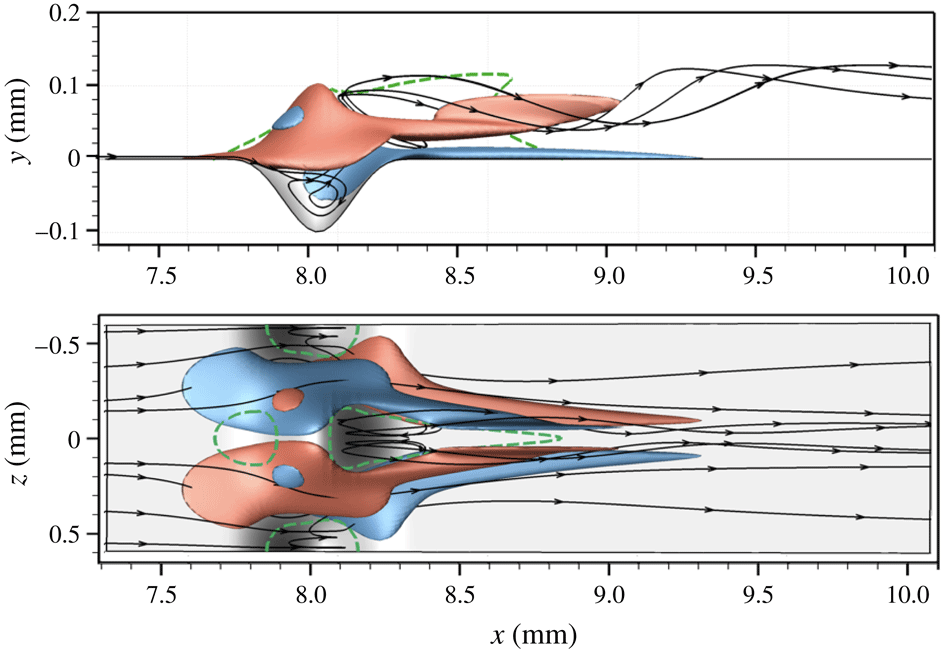
The roughness patch is characterised by three regions of separated flow, shown in figure 8 as dashed green lines. Two separation regions are located immediately upstream and downstream of the roughness protuberance. A third separation region is associated with the roughness cavities and is highlighted by the recirculating streamlines.
Isosurfaces of streamwise vorticity (red,
 $\unicode[STIX]{x1D714}_{x}=+10^{6}~\text{s}^{-1}$
; blue,
 $\unicode[STIX]{x1D714}_{x}=-10^{6}~\text{s}^{-1}$
) near the roughness patch. The flow-separation regions in the plane
 $z=0$
and on the wall are marked with the dashed green line.

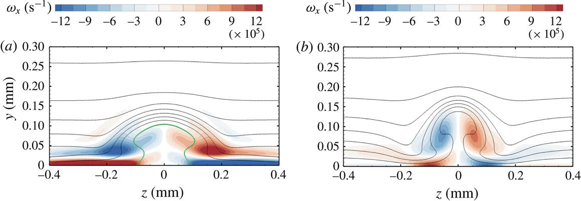
Figure 8 also shows isosurfaces of the streamwise vorticity. The roughness wake is mainly influenced by the protuberances rather than by the cavities. In particular, a pair of counter-rotating vortices originate at the sides of the roughness protuberance and the roughness wake resembles the one already observed in the case of isolated roughness elements. Through the lift-up mechanisms described by Landahl (Reference Landahl1980), these vortices induce movement of low-momentum fluid from the near-wall region upwards immediately behind the roughness protuberance. As a consequence, a low-speed streak originates along the protuberance centreline, as shown in figure 9. The rotation of the fluid around the vortex cores is visualised in figure 8 by the helicoidal shape of the streamlines in the near region of the roughness wake. Further downstream, as the vortices weaken, the flow pattern evolves into a mushroom-shaped geometry, as is known from the case of an isolated roughness element (Stemmer et al. Reference Stemmer, Birrer and Adams2017b ). Compared to the case of the smooth-wall geometry, the presence of the low-speed streaks is associated with a strong deformation of the flow and, hence, with regions of high shear stress, resulting in a potentially unstable wake.
Note that the flow variables and the shape of the wake rapidly change in the streamwise direction because of the strong acceleration of the base flow due to the hemispherical shape of the blunt body. Especially close to the roughness in the region of the separated flow, the boundary-layer properties change fast in the flow direction and parallel-flow assumptions in the stability analysis might not be valid.
Contours of the streamwise vorticity and streamwise velocity levels at
 $x=8.4~\text{mm}$
(a) and
 $x=9.2~\text{mm}$
(b). Values of the streamwise vorticity with an absolute value below
 $10\,\%$
of the absolute maximum value are blanked out. Velocity levels are shown every
 $50~\text{m}~\text{s}^{-1}$
. The zero-velocity line in (a) is marked in green.

3.2 Stability properties
The presence of unstable modes in the wake of the spanwise periodic roughness elements has been investigated with the help of LST-2D, PSE-3D and DNS. The results obtained with the different methods are compared for cross-validation. In the case of DNS, unsteady pressure perturbations with a frequency
 $f_{1}=250~\text{kHz}$
are introduced at the inflow, as described in § 2.2. As the boundary layer for the smooth-wall geometry is stable at the roughness location, the value of the disturbance frequency has been chosen based on numerical investigations of the base flow with a rough wall through LST-2D analysis.
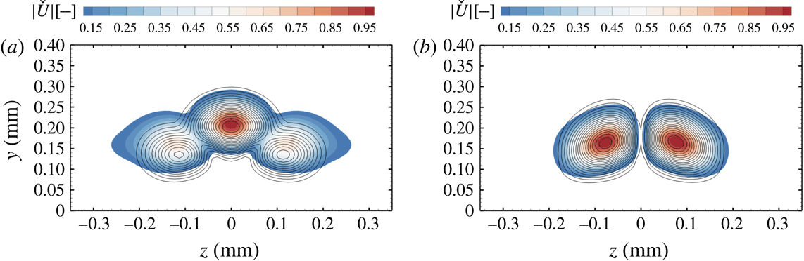
For the investigated frequency, the stability analysis evidenced the presence of two main unstable modes. As in the case of an isolated roughness element, a symmetric (S) and an antisymmetric (A) mode are present. The mode shapes for A- and S-modes of the streamwise velocity compared to DNS results are shown in figure 10. Modes from the DNS are obtained as absolute value of the temporal Fourier analysis.
Mode shape from DNS (black contour lines) and LST-2D (coloured contours). Results are shown for the S-mode (a) and the A-mode (b) at
 $x=18.5~\text{mm}$
. Values are normalised to unity and absolute values below
 $10\,\%$
of the absolute maximum value are blanked out.

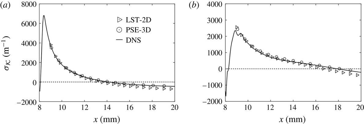
The value of the growth rate
 $\unicode[STIX]{x1D70E}_{{\mathcal{K}}}$
, computed with different numerical methods, is shown in figure 11. Analyses based on LST-2D and PSE-3D are limited to the flow downstream of the roughness only and do not include the recirculation region. Excellent agreement is observed for the results of DNS and PSE-3D in the S-mode case. In the A-mode case, a small difference between DNS and PSE-3D is observed close to the roughness patch downstream of the recirculation zone. We attribute this discrepancy to the difficulties of obtaining a mode in the roughness wake which is perfectly antisymmetric. In fact, the growth rates in the recirculation zone are much stronger for the S-mode than for the A-mode and a relatively small symmetric component was always present even in case of a pure antisymmetric inflow disturbance. Instead, an almost perfect match is reached further downstream. There is a small deviation between the curves of LST-2D and of PSE-3D. This discrepancy indicates that gradients in the flow direction of base flow and disturbance play a small but non-negligible role in the investigated region.
Growth rate of the S-mode (a) and A-mode (b) in the wake of spanwise periodic roughness elements.
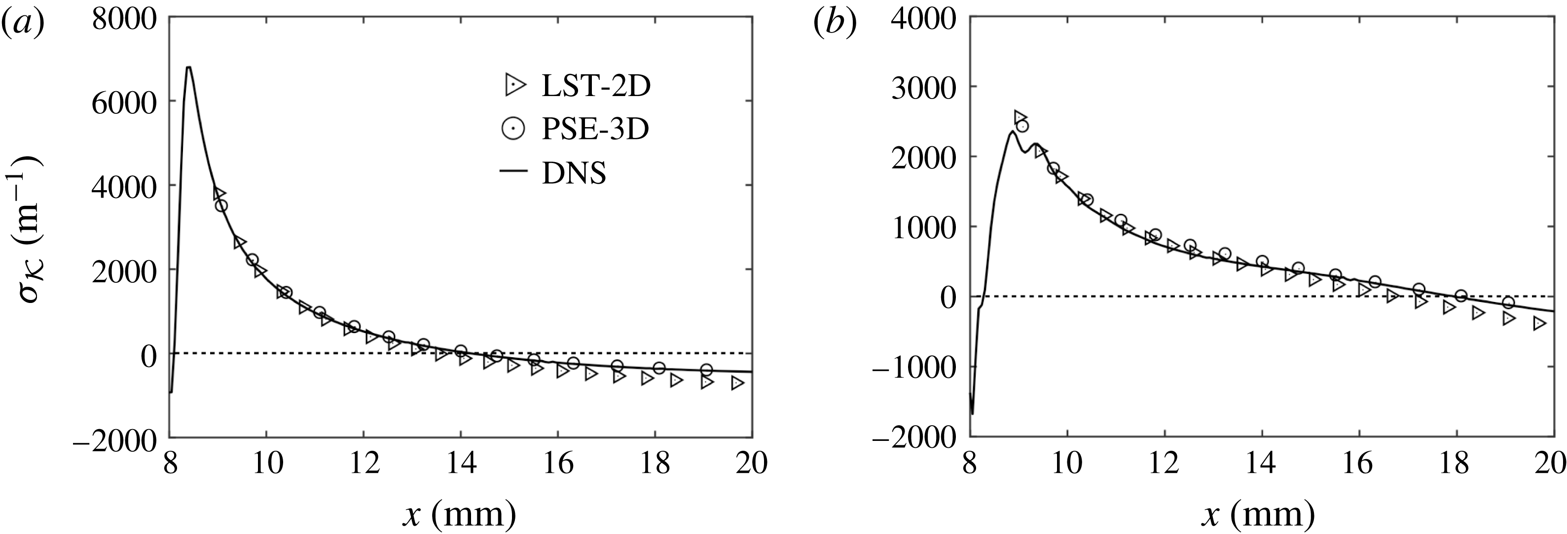
Even though larger values of the growth rate are reached for the S-mode, the A-mode remains amplified over a longer distance downstream of the roughness location. In particular, the zero growth rate is found at
 $x=14.2~\text{mm}$
for the S-mode and at
 $x=17.9~\text{mm}$
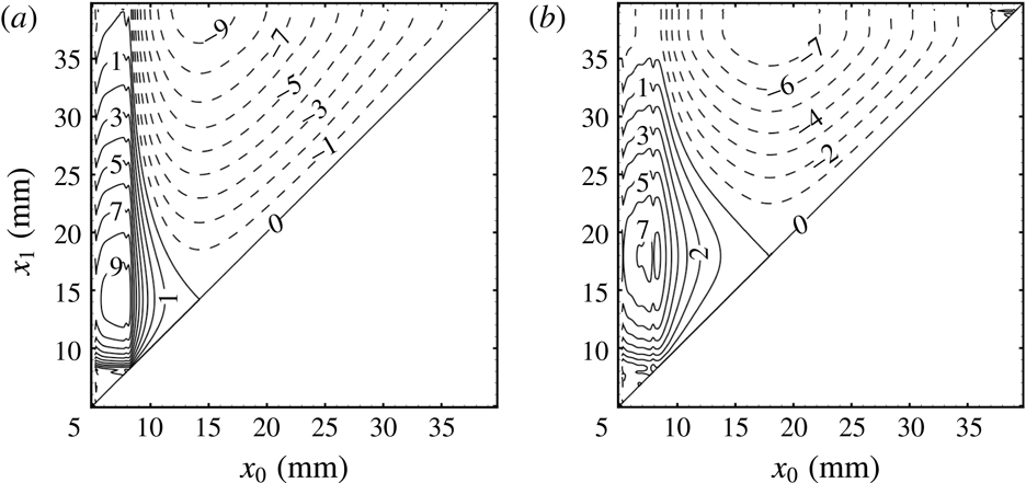
for the A-mode. This behaviour is better illustrated in figure 12, which shows a two-dimensional representation of the
 $N$
-factor as calculated from DNS results. The
 $N$
-factor is computed as
 $$\begin{eqnarray}N=\int _{x_{0}}^{x_{1}}\unicode[STIX]{x1D70E}_{{\mathcal{K}}}\,\text{d}x\end{eqnarray}$$
and is a function of both the start location
 $x_{0}$
and the end location
 $x_{1}$
. The largest value of the
 $N$
-factor for the S-mode is
 $9.6$
and is obtained for
 $x_{0}=7.7~\text{mm}$
and
 $x_{1}=14.2~\text{mm}$
, whereas for the A-mode the largest value of the
 $N$
-factor is
 $7.3$
and it is obtained for
 $x_{0}=7.7~\text{mm}$
and
 $x_{1}=17.9~\text{mm}$
. Note that for both the A- and S-modes, the value of
 $x_{0}$
for the maximum
 $N$
-factor turns out to be the same and it corresponds to a position just upstream of the roughness element, which starts at
 $x=7.75~\text{mm}$
. In this respect, the possibility of easily incorporating the flow over the roughness patch and the recirculation zone in the stability analysis can be regarded as one of the advantages of DNS.
Two-dimensional representation of the
 $N$
-factor as a function of both the initial and end positions (
 $x_{0}$
,
 $x_{1}$
) for the symmetric (a) and antisymmetric (b) mode.
 $N$
-factor isolines (solid for
 $N\geqslant 0$
and dashed for
 $N<0$
) are shown every
 $0.5$
.

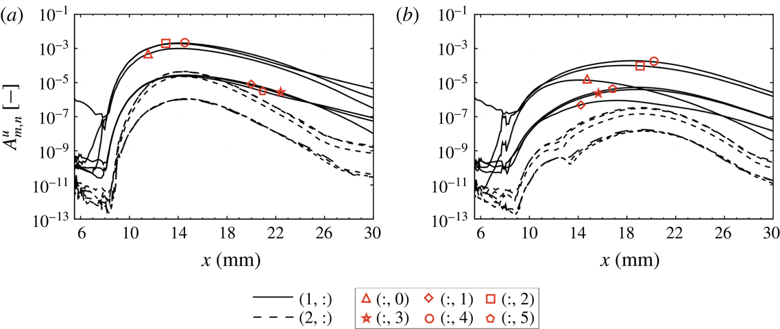
The amplitude development of the disturbance modes is shown in figure 13. The amplitudes are normalised by
 $U=359~\text{m}~\text{s}^{-1}$
, which is the boundary-layer edge velocity at
 $x=8~\text{mm}$
. At the inflow, only one particular perturbation mode is introduced. Specifically, (
 $1,0$
) is perturbed to generate the S-mode and (
 $1,2$
) is perturbed to generate the A-mode. At the roughness position, further modes with the same frequency, (
 $1,:$
), are generated. For both the S-mode and the A-mode, (
 $1,2$
) and (
 $1,4$
) are the most amplified spatio-temporal modes. Since (
 $1,2$
) corresponds to a wave with a spanwise wavelength equal to the roughness wavelength
 $\unicode[STIX]{x1D706}_{0}$
, the mode (
 $1,1$
) represents a subharmonic of (
 $1,2$
). Note that values of (
 $1,1$
) remain several orders of magnitude lower than the most relevant modes over the entire range. Additional modes with multiple frequencies (
 $2,:$
) are generated through superposition of the modes (
 $1,:$
) due to nonlinear interactions.
Amplitude of disturbance Fourier modes of the streamwise velocity for the symmetric (a) and antisymmetric (b) unstable modes.

4 Results for the randomly distributed roughness
4.1 Laminar base flow with a cross-flow-type vortex
In the case of a patch of randomly distributed roughness (figure 7), the concurrent effect of protuberances and cavities of different size, shape and streamwise profile can be investigated. Figure 14 shows a representation of the rough wall with elevation isocontours seen from the top. The eight main roughness peaks are marked with numbers
 $1$
–
 $8$
and their properties (e.g. height, position on the wall, height to boundary-layer thickness ratio and local
 $Re_{kk}$
) are summarised in table 5. The highest roughness peak has an elevation of
 $k=0.1~\text{mm}$
and the relative roughness Reynolds number is
 $Re_{kk}=406$
. The other peaks marked in the figure have an elevation of between
 $0.039~\text{mm}$
and
 $0.062~\text{mm}$
and roughness Reynolds numbers between
 $87$
and
 $191$
. To give an insight into the flow topology, sample streamlines and flow recirculation regions are shown. The presence of recirculation regions seems to be related both to the height of the roughness and to its shape as well as to its alignment with the flow. In particular, the shape of both peaks
 $2$
and
 $4$
is elongated in the flow direction and the flow remains attached as it passes over these protuberances. Instead, the smaller protuberances
 $6$
,
 $7$
and
 $8$
are mainly elongated in the cross-flow direction and are followed by cavities that promote the formation of recirculation regions.
Representation of the rough wall with streamlines. Separation regions on the wall are marked in green.

Three-dimensional representation of the flow field over the distributed roughness patch. Downstream slices at
 $x=8.6~\text{mm}$
and
 $x=15.9~\text{mm}$
and sample streamlines (a–d) are coloured by streamwise vorticity.

Colour contours of the streamwise vorticity and streamwise velocity isolines at
 $x=8.6~\text{mm}$
; values of the streamwise vorticity with an absolute value below
 $10\,\%$
of the absolute maximum value on the same plane are blanked out and velocity levels are shown every
 $25~\text{m}~\text{s}^{-1}$
.

Position (
 $x,z$
) and local roughness variables with reference to the main roughness peaks marked in figure 14.

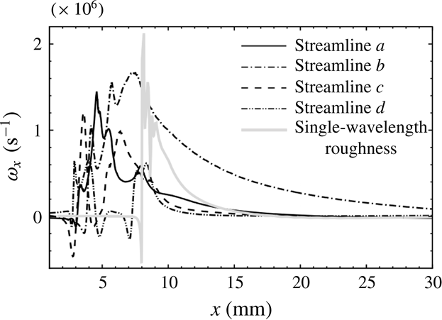
As in the case of the spanwise periodic roughness elements, the roughness peaks produce streamwise vortices. Figure 15 shows four streamlines passing over the roughness and centred on the main vortex cores downstream of the patch. At the vortex core, vorticity and velocity tend to align and, therefore, the vortex lines are to a good approximation identical to the streamlines (Levy, Degani & Seginer Reference Levy, Degani and Seginer1990). The streamlines allow us to track the evolution of the flow in the upstream direction back to positions upstream of the roughness. The streamlines are coloured by the value of the streamwise vorticity. The interaction of the flow with subsequent peaks and valleys is evidenced by the alternation of high- and low-vorticity values along the same streamline. As the streamlines are deflected at the protuberance, the magnitude of the streamwise vorticity strongly increases. As expected, the main vortex developing downstream of the roughness originates from the highest protuberance (peak
 $1$
, streamline
 $b$
). Streamlines
 $a$
,
 $c$
and
 $d$
exhibit a high vorticity at the roughness position. This vorticity rapidly vanishes further downstream, as evidenced by the grey colour of the streamlines for
 $x>12~\text{mm}$
.
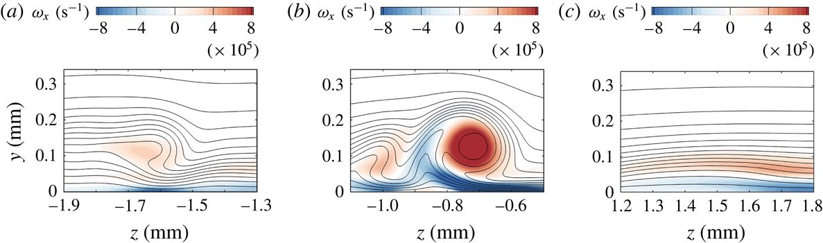
The vorticity distributions at three different positions in the same
 $y$
–
 $z$
plane downstream of the roughness patch (
 $x=8.6~\text{mm}$
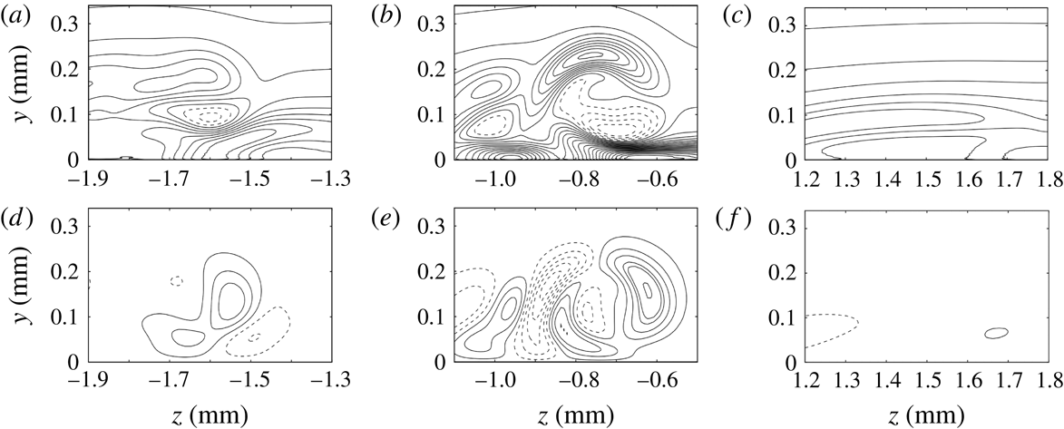
) are shown in figure 16. The distortion of the velocity flow field is evidenced by the rolling up of the isolines of streamwise velocity. The presence of a high-shear layer induced in the surroundings of the vortex is shown in figure 17, with isolines of the
 $y$
- and
 $z$
-components of the gradient of the streamwise velocity,
 $\unicode[STIX]{x2202}u/\unicode[STIX]{x2202}y$
and
 $\unicode[STIX]{x2202}u/\unicode[STIX]{x2202}z$
.
Of particular interest is the steady cross-flow-type vortex which develops in the wake of peak
 $1$
(figure 16
b). The skewness of the roughness relative to the streamwise flow induces velocity and vorticity distributions known from cross-flow vortices in three-dimensional boundary layers (streamline
 $b$
). The cavity downstream of peak
 $1$
contributes to the vortex generation with a further increase of the local wall-normal component of the velocity. High values of both
 $\unicode[STIX]{x2202}u/\unicode[STIX]{x2202}y$
and
 $\unicode[STIX]{x2202}u/\unicode[STIX]{x2202}z$
are found around this vortex structure (figure 17
b,e). The presence of this high-shear layer is associated with highly unstable modes. Cross-flow vortices in three-dimensional boundary layers have been extensively studied in the past and detailed numerical studies of cross-flow instabilities are presented, among others, in Malik, Li & Chang (Reference Malik, Li and Chang1994), Malik et al. (Reference Malik, Li, Choudhari and Chang1999) and Wassermann & Kloker (Reference Wassermann and Kloker2002). However, in the case of cross-flow vortices in three-dimensional boundary layers, a spanwise velocity is present in the base flow. Instead, the flow in the present configuration without roughness is two-dimensional and the spanwise component of the velocity typical of cross-flow vortices is directly induced by the roughness itself. In the works of Kegerise et al. (Reference Kegerise, King, Choudhari, Li and Norris2014) and Choudhari et al. (Reference Choudhari, Li, Bynum, Kegerise and King2015), similar roughness-induced cross-flow-type vortices have been observed for the case of a supersonic, flat-plate boundary layer in the presence of an isolated roughness element with a triangle shape. Contrary to the case of a flat plate, the hemisphere configuration with a smooth wall does not support modal instabilities and the roughness can be regarded as the only cause of significant disturbance growth.
On the left side of the cross-flow-type vortex, there is a minor vortex centred at
 $z\approx -1.0~\text{mm}$
, corresponding to the streamline
 $c$
. A third vorticity region is shown in figure 16(a). This vortex originates at peak
 $8$
and streamline
 $a$
evolves from this peak. A sudden increase of the streamwise vorticity occurs downstream of the protuberance. Here, an additional wall-normal component of the velocity is introduced by the presence of the cavity between peaks
 $1$
and
 $8$
.
Finally, streamline
 $d$
shows the subsequent effects of peaks
 $6$
and
 $2$
on the flow. After a slight increase immediately downstream of peak
 $6$
, the value of the streamwise vorticity rapidly falls. A second increase of the vorticity is found at peak
 $2$
at the end of the roughness patch. Although this roughness protuberance has a non-symmetric profile alignment similar to that of peak
 $1$
, its height is too small to give birth to a significant vortex (figure 16
c).
Isolines of
 $\unicode[STIX]{x2202}u/\unicode[STIX]{x2202}y$
(a–c) and
 $\unicode[STIX]{x2202}u/\unicode[STIX]{x2202}z$
(d–f) at
 $x=8.6~\text{mm}$
. Lines are shown every
 $400~\text{s}^{-1}$
and dashed lines represent negative values.

The downstream evolution of the streamwise vorticity
 $\unicode[STIX]{x1D714}_{x}$
along these streamlines is shown in figure 18. The streamwise vorticity reaches its maximum at the roughness position with values in the range 1.0 and
 $1.7\times 10^{6}~\text{m}^{-1}$
and it diminishes rapidly downstream of the roughness. With the only exception being the cross-flow-type vortex, the other streamwise vortices vanish within a few millimetres downstream of the roughness patch. The cross-flow-type vortex remains at a considerable amplitude in the computational domain until the outflow boundary is reached. The persistence of the cross-flow-type vortex is mainly related to its specific shape rather than to the height of the roughness peak
 $1$
. The development of
 $\unicode[STIX]{x1D714}_{x}$
in the case of the spanwise periodic roughness elements is also shown for comparison. In this case, the two streamlines located in the cores of a counter-rotating vortex pair, as shown in figure 9, have been identified. The streamwise vorticity difference was computed as
 $\unicode[STIX]{x1D714}_{x}=1/2(\unicode[STIX]{x1D714}_{x}^{+}-\unicode[STIX]{x1D714}_{x}^{-})$
, where
 $\unicode[STIX]{x1D714}_{x}^{+}$
and
 $\unicode[STIX]{x1D714}_{x}^{-}$
refer to the maximum positive and negative vorticity. Although the maximum roughness height is the same as in the case of the distributed roughness, the vortices in the wake of the spanwise periodic roughness elements decay fast and are extinguished within a distance of approximately
 $10~\text{mm}$
downstream of the roughness position.
Values of the streamwise vorticity along the streamlines a–d as shown in figure 15.

4.2 Instability modes and breakdown scenario
The wake of the randomly distributed roughness is more complex than that of periodic roughness elements and is characterised by several vorticity regions with different modes of instability possibly interacting with each other. Analyses based on LST-2D and PSE-3D are impossible to conduct as the flow is locally non-periodic in the spanwise direction for the various isolated vortices in the roughness wake. The evolution of small perturbations over the patch of distributed roughness and in the roughness wake is investigated with DNS only. Compared to LST-2D and PSE-3D, the use of DNS allows for a more detailed analysis of the flow in the entire simulation domain, including the roughness patch. Moreover, the formation and evolution of secondary instabilities and the onset of laminar breakdown to turbulence can be investigated.
A two-dimensional pressure disturbance wave is forced at the inflow boundary. Free-stream conditions and roughness variables (roughness height, roughness Reynolds number and shortest roughness wavelength in the patch) are the same as in the case of spanwise periodic roughness elements. Therefore, the analysis is conducted with the same frequency
 $f_{1}=250~\text{kHz}$
as in § 3.
We accurately analysed the disturbance evolution downstream of each protuberance and cavity of the roughness patch and found that the only appreciable disturbance amplification is associated with the steady cross-flow-type vortex presented in § 4.1. This vortex is responsible for a prolonged and strong disturbance amplification which, eventually, leads to transition. On the contrary, as the wakes of the other roughness peaks rapidly vanish in the strongly accelerated boundary layer, no significant amplification is observed in these wakes at the investigated frequency.
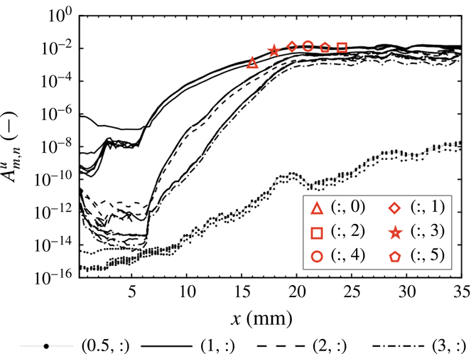
The downstream development of the Fourier amplitudes is presented in figure 19. The mode (
 $1,0$
) corresponds to the inflow disturbance. Modes with the same frequency but different wavenumbers are generated at the roughness location. Modes (
 $1,:$
) rapidly grow in the roughness wake, whereas higher harmonic frequency modes (
 $m>1,:$
) are generated due to nonlinear interactions. Eventually, a growth saturation of the base modes (
 $1,:$
) is reached for
 $x>17~\text{mm}$
, followed by a saturation of the higher frequency modes around
 $x\approx 18~\text{mm}$
. Downstream of this location, nonlinear interactions dominate the flow, leading to breakdown to turbulence. Subharmonic frequency modes (
 $0.5,:$
), i.e. modes with
 $125~\text{kHz}$
, remain negligible in amplitude over the entire domain. Furthermore, we note that, although disturbance growth is present at the roughness location, the onset of secondary instabilities occurs in the roughness wake downstream of the patch. Since linear as well as nonlinear growth of the disturbances to transition is the focus of our analysis, investigation of the pseudo-turbulent flow is not presented here and the flow for
 $x>25~\text{mm}$
has to be considered as not fully resolved.
Amplitude of spatio-temporal Fourier modes of the streamwise velocity in the case of distributed roughness. Values are normalised with the velocity at the boundary-layer edge
 $U=359~\text{m}~\text{s}^{-1}$
.

The instability of the boundary layer originates in the high-shear layer in the vicinity of the vortex and in the corresponding inflection points. In particular, the increase of disturbance kinetic energy associated with the growth of unstable modes is mainly due to energy transfer through wall-normal and spanwise velocity gradients. To investigate whether instabilities in the present case originate from wall-normal or spanwise gradients similar to the
 $y$
- and
 $z$
-modes in three-dimensional boundary layers (Wassermann & Kloker Reference Wassermann and Kloker2002), we analyse the two main production terms
 $P_{y}$
and
 $P_{z}$
in the disturbance kinetic energy,
 $$\begin{eqnarray}P_{y}=-\overline{u^{\prime }v^{\prime }}\frac{\unicode[STIX]{x2202}\overline{u}}{\unicode[STIX]{x2202}y},\quad P_{z}=-\overline{u^{\prime }w^{\prime }}\frac{\unicode[STIX]{x2202}\overline{u}}{\unicode[STIX]{x2202}z},\end{eqnarray}$$
where the overbar denotes the time average and the prime a fluctuating quantity. Local values of
 $P_{y}$
and
 $P_{z}$
at consecutive
 $x$
positions in the roughness wake are shown in figure 20. For clarity purposes, values of
 $P_{y}$
and
 $P_{z}$
at each
 $x$
position are normalised with the maximum value of the total production term
 $P=P_{y}+P_{z}$
in the
 $y$
–
 $z$
plane. Also shown are the disturbance modes of the streamwise velocity, computed from DNS for the frequency
 $f_{1}$
.
In the near-field region (figure 20
a,b), the disturbance mode of the streamwise velocity appears as a single, elongated and curved shape wrapped around the cross-flow-type vortex. As this mode evolves downstream, two main instability regions of elliptical shape become evident. The evolution of the disturbance mode in the streamwise direction correlates well with the main regions of disturbance-energy production (colour isocontours). In particular,
 $P_{y}$
identifies three regions of high disturbance production which resemble a distorted version of the S-mode analysed in § 3.2. Furthermore,
 $P_{y}$
seems to be related to the formation of the instability region visible in the upper-left corner of figure 20(c,d). The effects of
 $P_{z}$
are confined mainly to the descending (right) side of the vortex.
Unstable disturbance modes of the streamwise velocity (black contour lines every
 $0.1$
for values
 ${\geqslant}0.3$
), local values of
 $P_{y}$
(a,c,e) and
 $P_{z}$
(b,d,f) (coloured isocontours) and streamwise velocity levels (grey background isolines for every
 $10~\text{m}~\text{s}^{-1}$
) at
 $x=12.0~\text{mm}$
(a,b),
 $x=14.7~\text{mm}$
(c,d) and
 $x=16.8~\text{mm}$
(e,f).

The integrals of the production terms, obtained from the local
 $P_{y}$
and
 $P_{z}$
over the
 $y$
–
 $z$
plane, are shown in figure 21. Before transition occurs, the value of
 $P_{z}$
is slightly larger than the value of
 $P_{y}$
, indicating a major role of the lateral shear layer to the disturbance growth. However, the values of both terms remain of the same order of magnitude over the entire domain and neither
 $y$
-modes nor
 $z$
-modes can be regarded as dominant.
Integral values of
 $P_{y}$
and
 $P_{z}$
along the
 $x$
-direction.

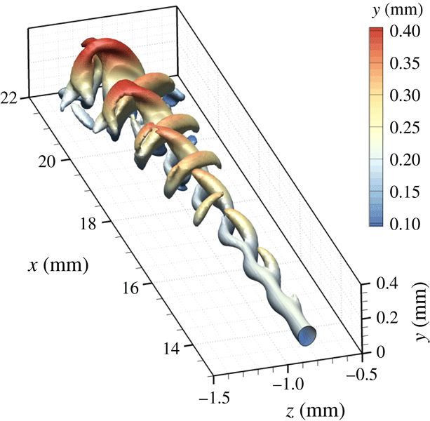
For the cross-flow-vortex breakdown, as analysed by Wassermann & Kloker (Reference Wassermann and Kloker2002), it was observed that the interaction between the steady vortex and the unsteady incoming disturbances gives birth to finger-like vortices wrapping around the ascending side of the steady vortex. Similar finger-like structures on the ascending (left) part of the vortex can be identified in the present simulation as well and are visualised by means of the
 $Q$
-isosurfaces shown in figure 22. The first appearance of these structures becomes visible at
 $x\approx 17~\text{mm}$
with a downstream wavelength of
 $1~\text{mm}$
, twining around the left side of the vortex centreline. However, another finger-like structure on the descending side of the steady vortex can also be seen. This structure, which occurs alternating with the one on the ascending side, gradually evolves into horseshoe vortices during the transition process. This mode of instability was not present in the work of Wassermann & Kloker (Reference Wassermann and Kloker2002) and, in our case, is obviously related to the region of large
 $P_{z}$
on the descending side of the vortex. In fact,
 $\unicode[STIX]{x2202}u/\unicode[STIX]{x2202}z$
presents a significant peak on the descending side of the vortex (figure 17
e, for
 $-0.7~\text{mm}<z<-0.5~\text{mm}$
), which was not found in Wassermann & Kloker (Reference Wassermann and Kloker2002).
Isosurfaces of
 $Q=3\times 10^{10}$
coloured by distance from the wall downstream of the roughness.

Representation of instantaneous disturbance pressure at the wall (a), vortical structures visualised with isosurfaces of
 $Q=3\times 10^{10}$
coloured by the distance from the wall (b) and instantaneous Stanton number (c).

Figure 23(a) shows the instantaneous value of the disturbance pressure
 $p^{\prime }$
at the wall, obtained as the difference between the unsteady and the steady simulations. The dominant streamwise wavelength of the disturbance can be retrieved by measuring the distance between two consecutive peak values of
 $p^{\prime }$
in the fishbone-like pattern. At the end of the roughness patch, the wavenumber of the disturbance is
 $\unicode[STIX]{x1D6FC}=6310~\text{m}^{-1}$
. With reference to
 $f_{1}$
, this wavenumber corresponds to a phase velocity of
 $c_{ph}=0.68U$
, where
 $U$
is the edge velocity of the boundary layer at the same position. No significant variation of the absolute value of
 $c_{ph}$
was found in the distance between the roughness and the onset of the secondary instabilities.
The transition location is also visible in the normalised heat flux at the wall (figure 23 c). The local, instantaneous Stanton number is calculated as
 $$\begin{eqnarray}St=\frac{\dot{q}}{\unicode[STIX]{x1D70C}_{\infty }U_{\infty }(H_{w}-H_{tot})},\end{eqnarray}$$
with
 $\dot{q}$
as the wall heat flux,
 $U_{\infty }$
and
 $\unicode[STIX]{x1D70C}_{\infty }$
the free-stream velocity and density,
 $H_{tot}$
the total enthalpy and
 $H_{w}$
the wall enthalpy. A significant increase of the Stanton number is observed in the roughness wake due to the distortion of the flow induced by the steady vortices. As the cross-flow-type vortex weakens, the Stanton number decreases. A further and sudden increase is observed for
 $x>21~\text{mm}$
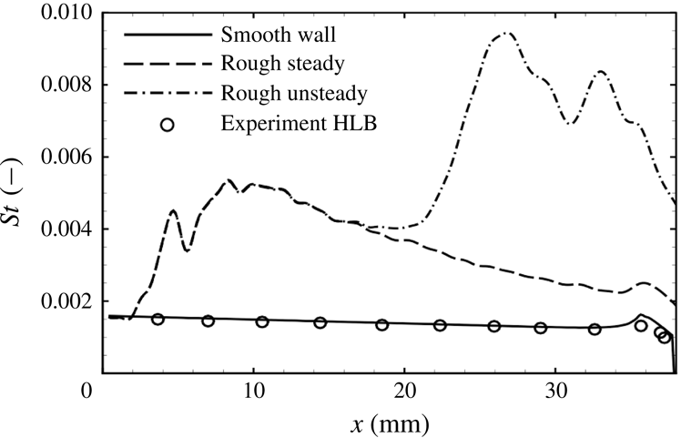
as a consequence of the ongoing laminar–turbulent transition. This behaviour is also illustrated in figure 24, which represents the maximum value in the spanwise direction of the time-averaged Stanton number found along the streamwise coordinate. The value of the Stanton number for the smooth wall configuration and for the steady simulation with a rough wall are shown for comparison. In addition, we represented the Stanton number measured in the experiments at HLB under the same free-stream conditions. These values are retrieved from Theiss et al. (Reference Theiss, Hein, Ali and Radespiel2016) for the capsule model with highly polished surface and correspond to the Stanton number measured close to the shoulder on the lee side of the capsule. In the case of the rough wall, the Stanton number significantly increases at the roughness location to 3–4 times the smooth values. For the steady rough-wall case, the value of the Stanton number starts to decrease for
 $x>10~\text{mm}$
. In the case of unsteady simulation, a deviation from the steady case is observed at
 $x>17~\text{mm}$
, corresponding to the point where secondary modes become important (cf. figure 19). The laminar–turbulent transition occurs further downstream and can be identified by the sudden and steep increase of the Stanton number occurring at
 $x\approx 22~\text{mm}$
. The Stanton number in the transition region rises to a threefold value compared to the steady rough case and can be significantly larger than the turbulent Stanton number.
Finally, we note that, in spite of the similar values of
 $Re_{kk}$
and
 $k/\unicode[STIX]{x1D6FF}$
for both geometries investigated, the roughness wake in the case of the distributed roughness leads to larger amplification rates compared to the case of spanwise periodic roughness elements. In the case of the distributed roughness, the modes undergo a longer and larger amplification, with an observed
 $N$
-factor with reference to the disturbance energy of approximately
 $13.2$
. In the case of the spanwise periodic roughness elements, the maximum amplification reached by the S-mode is smaller, with an
 $N$
-factor of
 $9.6$
.
Values of the Stanton number.

Colour contours of the streamwise vorticity and isolines of the streamwise velocity at
 $x=8.6~\text{mm}$
for distributed roughness with
 $k=0.025~\text{mm}$
(a),
 $k=0.050~\text{mm}$
(b) and
 $k=0.075~\text{mm}$
(c). Velocity levels are shown every
 $25~\text{m}~\text{s}^{-1}$
.

4.3 Simulations with different roughness heights
A parameter study with different roughness heights is carried out for the case of randomly distributed roughness. Different roughness patches are obtained by varying the value of
 $k$
in (2.5). Amplitude and phase coefficients are the same as in table 4. Three different roughness heights are additionally considered:
 $k=0.025$
,
 $0.050$
and
 $0.750~\text{mm}$
. The corresponding roughness parameters are listed in table 6.
Roughness variables for the distributed roughness investigated in the parameter study.

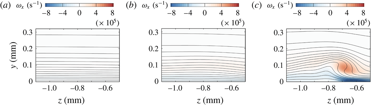
Figure 25 shows velocity and vorticity distributions in an
 $y$
–
 $z$
plane downstream of the roughness patch at
 $x=8.6~\text{mm}$
(cf. figure 16
b). Only in the case of
 $k=0.075~\text{mm}$
does the roughness wake present a vortical structure which induces a significant distortion of the base flow. In the case of
 $k=0.050~\text{mm}$
a slight warping of the velocity isolines is visible downstream of the roughness patch, whereas almost no influence of the roughness at the considered position is visible for
 $k=0.025~\text{mm}$
.
The amplitude of the modes of the streamwise velocity for the perturbed frequency
 $f=250~\text{kHz}$
is shown in figure 26. For clarity, only the mode (
 $1$
,
 $3$
) is shown (the same behaviour is observed for modes with same frequency and different wavenumber). The mode for the case of
 $k=0.100~\text{mm}$
is also shown for comparison. Only in the case of
 $k=0.075~\text{mm}$
does a significant amplification of the unsteady disturbance take place in the wake of the roughness. However, the roughness height is not large enough to generate a cross-flow-like vortex with characteristics similar to those analysed in § 4.2. As the generated vortex weakens downstream of the roughness patch, a positive growth rate of the disturbances is found in the vicinity of the roughness patch only. The observed
 $N$
-factor is 8.5. For roughness heights smaller than
 $0.050~\text{mm}$
, the disturbance amplification is limited in the region of the roughness patch only. The generation of the cross-flow-type vortex is of a nonlinear nature as the roughness has to be high enough to induce enough vorticity to keep the vortex alive. In the case of small roughness heights, the structures appearing are not cross-flow-like and are attenuated too fast to be the source of an instability mechanism. Only for
 $k=0.100~\text{mm}$
does this mechanism kick in and cause breakdown.
Amplitude of spatio-temporal Fourier modes (1, 3) of the streamwise velocity in the case of distributed roughness for different roughness heights. Values are normalised with the velocity at the boundary-layer edge
 $U=359~\text{m}~\text{s}^{-1}$
.

5 Summary and conclusions
This work presents analysis and in-depth description of roughness-induced instabilities in the highly accelerated boundary layer of a capsule-like hemispherical forebody at
 $M=5.9$
. Direct numerical simulations have been performed to study the development of disturbances with a frequency of
 $f_{1}=250~\text{kHz}$
introduced in the inflow boundary of the simulation domain. Previous studies showed that known instability mechanisms (such as TS-waves, Görtler-type instabilities, cross-flow instabilities and transient growth) cannot explain transition for the considered blunt-capsule configuration with a smooth wall. In this regard, the present work aimed at investigating the presence of instability mechanisms induced by roughness.
Two different types of roughness are analysed. In the first case, a spanwise periodic roughness element is modelled with a single-wavelength sinusoidal function of the surface. In the second case, the roughness patch is obtained by superposing different sinusoidal functions with pseudo-random amplitudes and phases. The maximum roughness height was
 $k=0.1~\text{mm}$
, with
 $k/\unicode[STIX]{x1D6FF}=0.35$
, for both geometries.
In the case of spanwise periodic roughness elements, two main unstable modes were found, corresponding to the symmetric and antisymmetric modes already known for the case of single roughness elements. The symmetric mode is more amplified than the antisymmetric mode if the recirculation zone is taken into account. An
 $N$
-factor of up to
 $9.6$
was found for the symmetric mode, whereas an
 $N$
-factor of up to
 $7.3$
was found for the antisymmetric mode. In the roughness wake, results from DNS were compared with results from PSE-3D analysis for validation and excellent agreement was achieved. Due to the strong acceleration of the flow, steady disturbances developing downstream of the roughness rapidly decay.
In the case of a randomly distributed roughness patch, the values of
 $Re_{kk}$
for the local roughness peaks ranged from
 $87$
to
 $406$
. The flow downstream of the roughness is characterised by separate vorticity regions, which originate at different peaks in the roughness. No significant amplification was observed in the wake of small roughness peaks with values of
 $Re_{kk}$
up to
 $191$
. The only appreciable disturbance amplification was found in the wake of the highest protuberance of the patch. Here, the skewness of the roughness together with the subsequent depression introduce a spanwise component of the velocity, giving birth to a new roughness-induced cross-flow-like vortex for the blunt-capsule configuration. The base flow for the smooth wall does not support modal cross-flow instabilities due to the insignificant component of the spanwise velocity. This cross-flow-type vortex greatly amplified the controlled unsteady disturbances introduced at the inflow boundary. The growth of the unsteady disturbances is characterised by the formation of finger-like vortical structures which wrap themselves alternatingly around both ascending and descending sides of the cross-flow-type vortex. Further downstream, these vortical structures evolve into horseshoe vortices and, eventually, lead to laminar–turbulent breakdown. The finger vortices on the descending side of the cross-flow-type vortex are related to high values of the spanwise velocity gradient and are not present in the cross-flow transition scenario in three-dimensional boundary layers.
Fourier modes of the forced frequency induce a nonlinear growth of higher frequency modes. The amplitude of higher modes reaches the amplitude of the forced modes at
 $x\approx 18~\text{mm}$
, where growth saturation is observed. However, analysis of the Stanton number at the wall showed that laminar–turbulent transition takes place further downstream, for
 $x\approx 22~\text{mm}$
, where a sudden and explosive increase can be observed.
The steady cross-flow-like vortex in the wake of the randomly distributed roughness is more persistent than the counter-rotating vortex pair in the wake of spanwise periodic roughness elements, in spite of the similar values of
 $Re_{kk}$
and
 $k/\unicode[STIX]{x1D6FF}$
. The vortices generated by the spanwise periodic roughness elements decay fast and are extinguished within a few millimetres downstream of the roughness position in the strongly accelerated boundary layer. On the contrary, the main vortex generated by the randomly distributed roughness remains at a considerable amplitude in the domain up to the outflow boundary. As expected, a larger
 $N$
-factor is found in the case of distributed roughness than in the case of periodic roughness elements. In fact,
 $Re_{kk}$
does not take into account either the roughness shape or the presence of cavities surrounding the roughness peak. It was shown that certain roughness shapes with a skew profile with respect to the flow direction can induce vortices similar to cross-flow vortices as known from three-dimensional boundary-layer flows. Their breakdown characteristics in the flow presented here resemble those known from three-dimensional boundary layers, where cross-flow vortices are a result of the stability properties of the flow with a spanwise velocity component. In the case analysed here, the roughness acts as a local source of spanwise velocity. The downstream evolution of the cross-flow-type vortices shows minimal decay, but the vortex strength is still large enough to exhibit instability towards artificial disturbances as introduced in this study.
A parameter study conducted for different roughness heights revealed that for
 $k/\unicode[STIX]{x1D6FF}\leqslant 0.263$
and
 $Re_{kk}\leqslant 261$
the vortex downstream of the roughness patch does not exhibit the characteristics of the cross-flow-type vortex. Because of the rapid decay of the vortex downstream of the roughness patch, the disturbance amplification is limited to the region close to the roughness, with an
 $N$
-factor of
 $N\leqslant 8.5$
for the investigated frequency. For re-entry vehicles, such as capsules with ablative TPS, the presence of distributed roughness is likely to be the normality rather than the exception. This work shows the necessity to account for roughness shapes on blunt bodies in the formulation of improved transition-prediction methods beyond
 $Re_{kk}$
-based criteria taking into account, e.g. spanwise and downstream gradients of the roughness elements as a measure. Other factors of influence still have to be investigated and their quantitative influence on the laminar–turbulent process revealed. The breakdown of the cross-flow-type vortex as described in this paper provides a possible explanation of laminar–turbulent transition on the capsule with distributed roughness in the absence of modal instabilities and insufficient transient-growth rates.
Acknowledgements
The authors gratefully acknowledge financial support through the German Research Foundation (Deutsche Forschungsgemeinschaft) under the contract STE 1454/8-2 and the computing and data resources provided by the Leibniz Supercomputing Centre (www.lrz.de). Data for figures 10 and 11 were gratefully provided by A. Theiss and S. Hein from the German Aerospace Center (DLR) Göttingen, Germany.