I. INTRODUCTION
Miedema and coworkersReference Miedema, de Chatel and de Boer1–Reference Miedema4 had proposed the following essentially empirical equation for the heat of formation ΔH of intermetallic phases:

where φ is proportional to Pauling’s electronegativity; N (in “density units”) was called “electron density at the boundary of the Wigner–Seitz cells” of the elements.Reference Miedema, de Chatel and de Boer1 “Δ” denotes the difference in two quantities for the two elements forming an alloy.
Rajasekharan and Girgis (RG)Reference Rajasekharan and Girgis5, Reference Rajasekharan and Girgis6 had observed that binary systems with intermetallic compounds of the same crystal structure occur along a straight line on a (Δφ,ΔN 1/3) map, referred to hereafter as the RG map. Considering 96 structure types with ∼3000 compounds,Reference Rajasekharan and Seshubai7–Reference Kameswari9 it has been demonstrated that Δφ ∝ ΔN 1/3 with a slope  for all the structure types. Binary systems with compounds of 88 of the structure types formed single straight lines and six of them formed dual lines, whereas AuCu3 and NaCl structure types formed multiple lines. The resolution on the map between the lines belonging to different structure types is good enough to anticipate many observations that can be made from binary metallic phase diagrams. An example is predicting the total absence of A15 type, NiAs type, and γ phase compounds from ∼250 binary systems in which the Laves phase compounds exist.Reference Rajasekharan and Girgis5, Reference Rajasekharan and Seshubai7, Reference Kameswari9 Another example is the prediction of 22 structure types including CaCu5 (hP6), FeB (oP8), Er2Co7 (hR18), Ce2Ni7 (hP36), NbBe3 (hR12), CFe3 (oP16), and Si3Mn5 (hP16) as possible concomitants to MgCu2 type compounds in binary systems.Reference Kameswari, Seshubai and Rajasekharan8 Since the choice of one crystal structure or another by intermetallic compounds is expected to be decided by small energy differences, the above observations are quite surprising.
It has been argued elsewhere that the above observations point to the possibility that in all compounds that coexist in a metallic binary system, irrespective of the crystal structure of the compounds, the energy of the nearest-neighbor unlike atom-pair bond remains the same. Several arguments in support of the above view have been published recently.Reference Rajasekharan and Seshubai7
In this study, we discuss the physical effects involved in the formation of an unlike atom-pair bond in an alloy. We then derive an equation for the energy of such a bond.
II. THE ENERGY OF THE ATOM-PAIR BOND
A. Basic assumptions
The covalent bonds in metallic alloys have to be different in two ways from a conventional chemical bond. First, while molecular compounds adjust their stoichiometry and conformation to avoid like charges in the immediate neighborhood, there has to be a charge transfer on the metallic bond due to the electroneutrality principle.Reference Pauling10 Second, there could be differences in the way the nuclear charges are screened by the electrons of an atom in a metal. The electron distribution in metals is usually approximated as the localized core electrons occupying a relatively small spherical volume around the nuclei, at the lattice points in the crystal, with the valence electrons distributed uniformly in the remaining region. If there are N valence electrons per atom, N 1/3 electrons can be expected to be on a linear bond, on an average. The valence effective on a linear bond would be N 1/3, the number of electrons available as a time average on the bond, as per the above equation. In this study, we hypothesize the screening of nuclear charges by the electrons of an atom in a metal is such that the effective charge felt by a valence electron situated at the midpoint of the bond to the next atom is N 1/3, i.e., all except N 1/3 electrons exert their full screening power. This means that at any moment in time, all electrons of the atom except N 1/3 are distributed with spherical symmetry in positions closer to the nucleus than at the midpoint of the bond. As is done with various hypotheses on screening by electrons in different physical situations,Reference Slater11 this assumption needs to be proven by comparison of its predictions with experimental results.
B. Equation for the energy of the atom-pair bond
Consider two atoms A and B of electronegativity χ A and χ B and valence N A and N B, with χ A > χ B. The atom with the higher electronegativity has often the higher valence,Reference Pauling10 so N A > N B. A compound forms by the breakage of homonuclear A–A and B–B bonds and the formation of A–B bonds. The bond formed between A and B will have a certain ionic character, and the increase in stability of the heteronuclear bond A–B in comparison with the average of the homonuclear bonds can be attributed to the ionicity in the bonds. The negative contribution to the bond energy due to this effect is equal toReference Pauling12, Reference Jolly13

PaulingReference Pauling10 pointed out that in metallic compounds, maximum stability would result from equalizing the number of valence electrons on A and B, thus maximizing the number of bonds between A and B by a transfer of electrons from A to B. Thus, the number of electrons/atom on the atom-pair bond after electron transfer would be 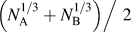 . The number of electrons transferred would then be
 .
The ionicity of the bond deposits extra negative charges near the more electronegative atom A, making the atom B positively charged. The electroneutrality principle would necessitateReference Pauling10 in metallic solids, charge transfer from A to B so that there are no net positive charges on B. We, therefore, infer that the charge transfer, i.e. (ΔN 1/3/2), from A to B has to increase with an increase in the electronegativity difference (Δχ) between the atoms on the A–B bond.
The transfer of electrons is from an atom with higher electronegativity χ A to one with lower electronegativity χ B and would make a positive contribution to the bond energy. The energy involved in removing an electron from an atomReference Mulliken14, Reference Mulliken15 is  , and hence the positive contribution is

where I A and E A in electron volts are the first ionization energy and electron affinity, respectively, of atom A and I B and E B are those of atom B. ΔH +ve is the difference in energy in electron volt, involved in the removal of (ΔN 1/3/2) electrons from the more electronegative atom A and its subsequent absorption by atom B.
We use the equationReference Huheey16 χ = 0.187 (I atom + E atom) + 0.17 connecting Pauling’s electronegativity values (χ) and  to write the total energy of the atom-pair bond, with Δχ = (χ A − χ B), as

It follows from Eq. (4) that the energy of the atom-pair bond would be negative if (Δχ/ΔN 1/3) > 1.34.
Above, we have obtained an equation for the energy of the metallic unlike atom-pair bond in terms of the average or lumped constants, electronegativity and valence of metallic elements. To apply the equation, we need to have values for the electronegativity and valence of elements in the metallic state. In the following paragraph, we have shown that Miedema’s electronegativity and “electron density at the boundary of the Wigner–Seitz cells of the atoms” might be identified with the electronegativity and valence of metallic elements, for the purpose.
C. On the valence and electronegativity of metallic elements
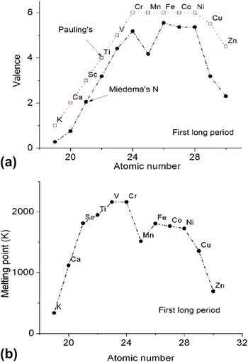
PaulingReference Pauling17, Reference Pauling18 had defined valences for metallic elements (say, N P) by studying the variation of their physical properties such as melting points, boiling points, hardness, etc., as function of their atomic number. As the valence and, thereby, the number of bonds between the atoms increase, properties such as melting points, boiling points, hardness, etc., also increase. Miedema et al.’s electron density parameter N, originally derived from the bulk modulus of elements, and then adjusted numerically so as to reproduce the correct signs of the heats of formation of binary metallic systems, are numerically close to N P. In Fig. 1(a), we show how N P and N vary with atomic number in the first long period of the periodic table. In Fig. 1(b), we show how the melting points of the elements vary across the same period. Comparison between Figs. 1(a) and 1(b) shows that the variation in Miedema’s parameter N reproduces the variation in the melting points more closely than does Pauling’s valences, including the anomalous behavior of Mn. Similar observations can be made from other periods of the periodic table also. This suggests that the numerical values of N might be considered as better choice for the valence of metallic elements, in comparison with N P.
Comparison of Miedema’s N with Pauling’s valences (N P) for metals. (a) We see that, in the first long period of the periodic table, Miedema’s N are comparable in magnitude and vary in the same way with the atomic number of the elements, as do Pauling’s valences. In (b), the melting points of the elements are plotted versus atomic number for elements of the first long period. We can observe from (a) and (b) that Miedema’s parameter N and the melting points of the elements vary in the same way with the atomic number of the elements in the period; the anomalous behavior of Mn is reflected in both.

PaulingReference Pauling19 had derived values of the electronegativity (χ P) of elements from the energy of their heteronuclear bonds. Electronegativity might be defined in an absolute way as the electrostatic potential due to nuclear charges of an atom, on a valence electron.Reference Gordy20 GordyReference Gordy20 could reproduce Pauling’s electronegativity values for 50 elements using the above definition, with an assumption that all the electrons in the closed shells below the valence shell exert their full screening power, and that the screening constant of one valence electron for another is 0.5. With the present assumption that all except N 1/3 electrons exert their full screening power in metallic elements, the electrostatic potential at the midpoint of the bond would be proportional to N 1/3/R, where R is the metallic radius of the atom. The electronegativity of a metallic atom would then be χ M = Z eff e/R = k N 1/3/R, where k is a constant.
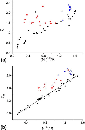
In Fig. 2(a), we show a plot of Pauling’s electronegativity χ of the metallic elements versus  . A very approximate linear dependence between the two can be observed. PaulingReference Pauling10 had divided metallic elements into three groups: hypoelectronic elements which have fewer electrons than there are orbitals, hyperelectronic ones which have more electrons than there are orbitals, and buffer elements. In Fig. 2(b), we show that an almost perfect (R = 0.98) linear correlation is obtained for hypoelectronic elements if one plots Miedema’s electronegativity values—which have been obtained by correcting Pauling’s values to suit the conditions existing in a metal—versus,
 , where N are Miedema’s corrected electron density parameters. The Miedema electronegativity values used above have been scaled down to the range of Pauling’s electronegativity values using the linear relationship between the two,

(a) A plot of Pauling’s electronegativity χ versus  is shown, where N P are Pauling’s valences for the metallic elements and R, the metallic radii. An approximate linear dependence between the two can be observed. The hypoelectronic transition metals, s-elements, and rare earths are shown as closed circles (black online), the p-metals which are hyperelectronic as unfilled squares (red online), and the buffer elements Ag, Au, Re, Ru, Os, Tc, Rh, Ir, Pt, and Pd as triangles (blue online). Pauling had classifiedReference Pauling10 the metallic elements as hypoelectronic, hyperelectronic, and buffer elements based on their electronic structure. (b) An excellent (R = 0.98) linear correlation is obtained for hypoelectronic elements if one plots Miedema’s electronegativity values (χ M) obtained after adjustment using the experimental information on the signs of the heats of formation of metallic binary systems versus N 1/3/R, where N are Miedema’s adjusted electron density parameters. The electronegativity values have been scaled down to the range of Pauling’s values without losing the information obtained by the correction process, by using the linear relationship given in Eq. (5), between the two.

The hypoelectronic elements consist of alkali metals, rare earths, and early transition metals. The improvement in linearity for hypoelectronic elements (black solid circles) in Fig. 2(b) which uses the corrected Miedema parameters is remarkable when compared with Fig. 2(a). In Gordy’sReference Gordy20 treatment, Cu, Ag, and Au were exceptions to the observed correlation. In Fig. 2(b), the buffer elements Ag, Au, Pt, Pd, Rh, Re, Os, and Tc (red squares) and the hyperelectronic p-metals (blue triangles) are found grouped separately from the hypoelectronic elements due to the difference in their electronic structure. The former are characterized by paired electrons in the final shell, which do not contribute to valence and could possibly contribute less to shielding and thus increase the electrostatic potential at the midpoint of the bond. It is interesting to note that Fig. 2(b) has separated out hypoelectronic, buffer, and hyperelectronic elements, and that their separation is an outcome of the adjustment in the values of electronegativity and electron density parameter based on the experimental information on the signs of ΔH. The observed linear correlation supports the hypothesis that χ M and N might be indentified with the electronegativity and valence, respectively, of metallic elements: the Miedema electronegativity of metallic elements can be calculated from their Miedema valences as the electrostatic potential at the midpoint of the bond.
III. DISCUSSION
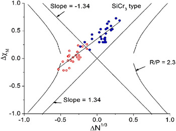
In Fig. 3, we show the intermetallic compounds crystallizing with the SiCr3 type crystal structure, with the t–p compounds marked by open circles (red online), on a map using Δχ M and ΔN 1/3 as coordinates. The straight lines with slopes ±1.34 representing ΔH Bond = 0 in Eq. (4) are also shown. The list of compounds crystallizing with SiCr3 type structure is from standard compilations.Reference Pearson21–Reference Massalski23 The compounds occur on a straight line (the Rajasekharan—Girgis lineReference Rajasekharan and Seshubai7) on the map. All the compounds except t–p compounds occur in the region where Δχ/ΔN 1/3 > 1.34, i.e., where, according to Eq. (4), ΔH Bond is negative. The t–p compounds are exceptions because, as discussed below, they are stabilized by an additional mechanism due to the increased valence on p-metals due to electron-pair breaking.
The compounds belonging to SiCr3 structure type are shown on a (Δχ M,ΔN 1/3) map. The lines of slope ±1.34, which separate regions of negative bond energy from those of positive bond energy according to Eq. (4), are shown. Each point on the map stands for a binary system. The compounds of hyperelectronic p-metals (open circles, red online) have an additional stabilizing mechanism due to electron-pair breaking. They are seen to occur in a region otherwise predicted to have positive bond energy by Eq. (4). The hyperbola corresponds to Miedema’s R/P = 2.3, which is equivalent to an additional stabilization of 2.3/4.65 = 0.5 eV [see Eq. (6)].

We note that the R/P term for t–p compounds in Miedema’s Eq. (1) also follows from the mechanism, which is proposed in this study. The hyperelectronic elements (mostly, p-metals) have more electrons than there are orbitals and hence have electrons paired up in their orbitals.Reference Pauling10 According to the present model, an amount of charge equal to ΔN 1/3/2 would be transferred from the higher electronegativity atoms, i.e., the p-metal atoms in the case of t–p combinations, to the lower electronegativity atoms. This would generate from electron-pair breaking an additional number of valence electrons on the p-metal atoms equal to ΔN 1/3/2 leading to increased stability by the formation of additional bonds. This mechanism accounts for the (R/P) term proportional to the valence of p-metals, found necessary by Miedema et al. to correctly predict the signs of the heats of formation of t–p combinations.
In a given binary system A–B, the heat of formation of compounds at the compositions AmBn (m < n) can be expected to vary roughly proportional to the number of A–B bonds that can form in the compounds, i.e., proportional to (m/(m + n)). This variation is similar to the experimentally observed variation of ΔH with composition in binary systems and is similar to the assumed f(c) in Eq. (1).
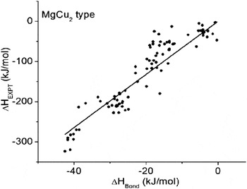
In Fig. 4, we show a plot of ΔH EXPT versus ΔH Bond calculated using Eq. (4), for MgCu2 type compounds. The experimental values of the heats of formation of MgCu2 type compounds ΔH EXPT were obtained from a review.Reference Zhu, Liu, Pike and Liaw24 The regression factor of the linear fit is 0.96. The experimental data included in Fig. 4 were obtained by a variety of techniques by different groups, and the ones obtained by the solution technique are expected to have better accuracy while the others could show a larger scatter.Reference Zhu, Liu, Pike and Liaw24 The heats of formation of new compounds of the above structure type can be obtained by interpolation from the linear plot. We note that there are no empirically derived constants in Eq. (4).
The experimentally determined heats of formation ΔH EXPT (kilojoule per mol) of MgCu2 type compounds are compared with the bond energy ΔH Bond (kilojoule per mol) calculated using Eq. (4). The energy obtained in electron volt per bond using Eq. (4) is multiplied by 96.485 to convert it into units of kilojoule per mol.

Equation (4) calculates the energy of the nearest-neighbor A–B bond only. The good correlation observed in Fig. 4 is due to the fact that major contribution to the heats of formation of intermetallic compounds arises from the nearest-neighbor unlike atom-pair interactionReference Rajasekharan and Seshubai7, and that is the reason why Eq. (4) predicts the signs of the heats of formation of intermetallic compounds accurately; if the unlike atom-pair bond energy goes positive in a compound, the compound would become unstable. The estimation of the heat of formation of a compound from the calculated bond energy requires multiplication by the number of nearest-neighbor bonds, consideration of the effect of resonance, and also the inclusion of the much smaller contributions of longer unlike atom-pair bonds to the total energy.
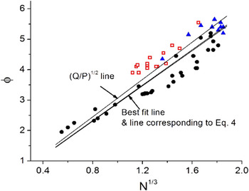
In Fig. 5, we plot φ versus N 1/3 for all the metallic elements. The best fit line through the origin (slope = 2.91) is shown in the figure. In Eq. (4) for the bond energy, if we replace χ by φ using Eq. (5) and substitute Δφ = 2.91 ΔN 1/3 in the second term, we get

A plot of φ versus N 1/3 for metallic elements. The best fit line through the origin with slope 2.91 and the line of slope (Q/P)1/2 = 3.07 are shown. The hypoelectronic elements are shown as closed circles (black online), the hyperelectronic elements as open squares (red online), and the buffer elements as triangles (blue online). According to Eq. (4), a line of slope 1.34 would separate binary systems with negative and positive heats of formation on a (Δχ M,ΔN 1/3) plot; this would correspond to a line of slope 2.89 on a (Δφ,ΔN 1/3) plot. The corresponding line is also shown in the figure.

The above equation is in the form of Miedema’s Eq. (1), with R/P = 0. According to the above equation, the slope of the line separating negative and positive ΔH Bond on a map using Δφ and ΔN 1/3 as coordinates would be 2.90. It is close to Miedema’s empirically derived slope (Q/P)1/2 = 3.07. ΔH Bond is the difference in two comparable quantities, and hence the corrections effected by Miedema et al. to their parameters become very significant.
IV. SUMMARY
In this study, we have derived an expression for the energy of an unlike atom-pair bond in a metallic alloy. The negative term in the expression is due to the ionicity in the bonds. PaulingReference Pauling10 had proposed charge transfer from the more electronegative atom to the less electronegative one for maintaining the electroneutrality in metallic alloys, but the energy cost of such charge transfer had not been considered in earlier approaches. In this study, we have quantified the positive contribution from such charge transfer to the equation for the energy of the bond. The resulting equation predicts the signs of the heats of formation of metallic alloys accurately. Miedema’s empirical constant (Q/P)1/2 follows from the proposed model.
It is of interest in the present context that an ab initio application of Pauling’s resonating valence bond (RVB) theory to Li atom clusters brings out the covalent character of the metal–metal bond and the importance of the metallic orbital.Reference Mohallem, Vianna, Quintao, Pavao and McWeeny25 Diffusion quantum Monte Carlo simulations of Li clusters show that RVB pairing correlations between electrons provide a substantial contribution to the cohesive energy.Reference Nissenbaum, Spanu, Attaccalite, Barbiellini and Bansil26 Elsewhere,Reference Harcourt and Styles27 valence-bond studies of aspects of electron conduction along a linear chain of lithium atoms have been reported. The present study uses average properties of elements such as electronegativity and valence to predict the behavior of metallic materials. The advantage of the present approach, as of conventional chemistry, is its easy applicability to problems in the laboratory/industry to relatively more complex systems, without recourse to long calculations. One of the uses of the equation for the energy of the atom-pair bond as developed in this study is in predicting a small set of hypothetical crystal structures for a given compound using the (Δχ M, ΔN 1/3) map. Those structures might be further investigated by the ab initio method to obtain the stable structure. Additionally, the approach helps in clarifying the role of various physical interactions in the alloying of metals.
ACKNOWLEDGMENT
T. Rajasekharan acknowledges the Defence Metallurgical Research Laboratory, Hyderabad, India, for giving permission to publish this article.