1 Introduction
Two-phase plumes, produced by the release of bubbles at the base or particles at the top of a body of fluid, are of considerable importance in the environment and industry. Bubble plumes are deployed for the destratification of lakes (Lemckert & Imberger Reference Lemckert and Imberger1993; Neto, Cardoso & Woods Reference Neto, Cardoso and Woods2016); particle plumes are generated when waste material is discharged into the ocean during deep-sea mining operations (Coulin et al. Reference Coulin, Haley, Jana, Kulkarni, Lermusiaux and Peacock2017); and submarine oil and gas blowouts have the potential to generate very significant two- and three-phase plumes which control the ascent and ultimate dispersal of the oil and gas (Johansen, Rye & Cooper Reference Johansen, Rye and Cooper2003; Socolofsky, Adams & Sherwood Reference Socolofsky, Adams and Sherwood2011).
There have been a number of experimental and theoretical investigations of the dynamics of bubble plumes (McDougall Reference McDougall1978; Milgram Reference Milgram1983; Asaeda & Imberger Reference Asaeda and Imberger1993; Socolofsky & Adams Reference Socolofsky and Adams2005). It has been shown that if the rise speed of the bubbles is small compared to that of the plume, then the flow largely follows that of a single-phase plume. However, once the rise speed of the bubbles exceeds the plume speed, the bubbles begin to separate from the flow. McDougall (Reference McDougall1978) described the motion of such bubble plumes in terms of an inner, bubble-rich core surrounded by an outer, bubble-poor zone, and developed a two-layer plume-type model to describe the flow. Asaeda & Imberger (Reference Asaeda and Imberger1993) showed that if a bubble plume rises through a stratified environment, then on reaching the neutral buoyancy height some of the bubble–fluid mixture detrains and spreads radially. Asaeda & Imberger proposed that as the bubbles separate from this intrusion, they may form a new plume, which carries ambient fluid upwards until it reaches a second neutral height. They suggested that the process may repeat multiple times, and a series of complex detrainment events are predicted as the bubbles rise through the water column. Socolofsky & Adams (Reference Socolofsky and Adams2005) proposed three flow regimes for such plumes depending on the ratio
 $U=v_{s}/(B_{0}N)^{1/4}$
between the rise speed of the bubbles,
 $v_{s}$
, and the characteristic speed of the plume,
 $(B_{0}N)^{1/4}$
, where
 $B_{0}$
is the source buoyancy flux of the plume and
 $N$
the ambient stratification: for
 $U<1.5$
, regime 1 involves the formation of a series of intrusions above the source, with bubbles spreading into each intrusion, then separating to form a new plume, which intrudes higher up in the system; for
 $1.5<U<2.4$
, regime 2 involves a similar series of plume-intrusion structures, but the bubbles tend to remain in the core of the flow, and do not spread into the intrusions; and for
 $U>2.4$
, regime 3 involves an irregular and unsteady region of fluid above the neutral height, with a stream of bubbles rising through the core of this region. One of the complexities of such bubble plumes is that there may be a range of bubble sizes, including a dispersed volume of small bubbles and a population of larger bubbles, thereby giving a range of rise speeds. Furthermore, the distortion, break-up and detailed dynamics of the bubbles relative to the fluid can have an impact on the mixing and entrainment rate (Milgram Reference Milgram1983).
The height at which the fluid from such a plume ultimately intrudes into the ambient is an extremely important environmental problem, since the plume fluid may contain dissolved contaminants which originate from the bubbles or particles. The intrusion height of the plume fluid will determine where these dissolved contaminants eventually disperse in the ambient. However, determination of this height is complex since the bubbles or particles will eventually separate from the flow in the initial, laterally spreading neutral cloud. This will result in a change in the buoyancy of the flow, and so the final intrusion height may be different from that of the initial intrusion, which corresponds to the intrusion height of a single-phase plume (Morton, Taylor & Turner Reference Morton, Taylor and Turner1956). A second point of importance concerns whether there is any vertical transport of plume fluid beyond the first neutral cloud and through the subsequent series of intrusions. Much of the previous literature suggests that the process involves a series of plume-intrusion structures which develop as the flow continues (e.g. Asaeda & Imberger Reference Asaeda and Imberger1993, Socolofsky & Adams Reference Socolofsky and Adams2005, Seol, Bryant & Socolofsky Reference Seol, Bryant and Socolofsky2009). Socolofsky & Adams identify several classes of two-phase plume, including the so-called
 $1^{\ast }$
regime in which
 $U<1$
. For this regime, they present experimental data of the height of the top of the plume and the subsequent height of the first fluid intrusion. These show that the first intrusion occurs within a range of values from about 0.5 to 0.7 of the initial plume height. They then develop an empirical law relating the intrusion height to the top height as a function of
 $U^{\ast }$
(see their figures 5 and 6). Seol et al. (Reference Seol, Bryant and Socolofsky2009) present further data about this, finding that for
 $U^{\ast }=1.1$
, the ratio of the two heights is about
 $0.55\pm 0.05$
based on their figure 4(a).
In order to explore the intrusion depths of the fluid transported by two-phase plumes in more detail, while avoiding the complexity of the bubble size distribution in a bubble plume, in the present paper we explore the analogous problem of a descending plume of dense particles in which the particles have a single size (cf. Chan, Chow & Adams Reference Chan, Chow and Adams2015, Lippert & Woods Reference Lippert and Woods2018). Bush, Thurber & Blanchette (Reference Bush, Thurber and Blanchette2003) reported an experimental investigation of particle-laden thermals, which are produced by the release of a finite mass of particles and fluid. Although this contrasts with the present work in which we focus on a continuous source of particle-laden fluid, leading to the formation of a quasi-steady turbulent plume, there are some analogous effects associated with the separation of fluid and particles. In particular, Bush et al. (Reference Bush, Thurber and Blanchette2003) identified that in the case where the thermal speed exceeds the particle fall speed, then in a stratified environment, the thermal has a maximum descent distance below the source which coincides with the classical results of Morton et al. (Reference Morton, Taylor and Turner1956) for a single-phase thermal. However, as the flow then spreads laterally, the particles separate from the fluid in the thermal, which then rises back towards the source a distance equal to approximately 0.25 of the maximum depth of the thermal before spreading out at the ultimate neutral buoyancy height of the particle-free fluid. We illustrate an analogous process in particle plumes produced by a constant source of buoyancy, although as we show the quantitative details are different. We also illustrate the strong influence of the initial buoyancy of the source fluid as well as that of the particle load in controlling the final intrusion depth.
In our experiments, we focus on the case in which the fall speed of the particles is smaller than the characteristic plume speed,
 $U<1$
, so that on leaving the source, a turbulent buoyant plume develops. In the experiments, the particles are supplied as a dilute suspension, and we explore the motion of the plume fluid and the particles once they have reached the neutral buoyancy height. We develop new models for the ultimate intrusion height of the fluid phase of this initial plume in terms of the source buoyancy flux, distinguishing between the buoyancy flux associated with the particles and that associated with the source fluid. In exploring the controls on the intrusion height of the plume fluid once the particles have sedimented from the intrusion, we vary the buoyancy of the source fluid from values more buoyant to values less buoyant than the ambient fluid surrounding the source, while keeping constant the total buoyancy flux of the mixture of source fluid and particles. We also describe the motion in the region below the maximum height of the initial plume. We analyse a series of new experiments to show that in this region there is no net vertical transport of fluid, and the particles sediment as a cylindrical column in the fluid at their sedimentation speed. We also show that owing to the density difference between the fluid in the particle-laden cylindrical column and the surrounding ambient, a regular series of intrusions form around the edge of the column, which lead to the development of layers of high and low particle concentration in the sedimenting column. Finally, we discuss the implications of our results for both bubble and particle plumes in a number of contexts.
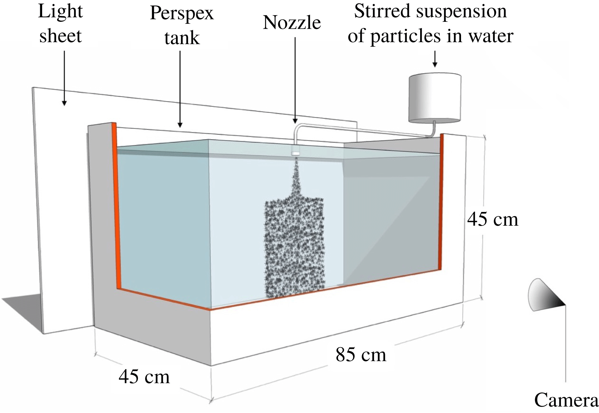
Schematic representation of the experimental set-up.

2 Set-up of experiments
A series of laboratory experiments were carried out in a perspex tank of dimensions
 $0.85~\text{m}\times 0.45~\text{m}\times 0.45~\text{m}$
(see figure 1). The tank was filled with an aqueous saline solution with a linear density stratification. The stratification was generated using the double bucket system (Oster & Yamamoto Reference Oster and Yamamoto1963) and tested by refractometer measurements of selected fluid samples before the beginning of each experiment (Atago Palette PR-32
 $\unicode[STIX]{x1D6FC}$
digital refractometer, accuracy of
 $\pm 0.1\,\%$
). The density of the fluid at the top of the tank,
 $\unicode[STIX]{x1D70C}_{a,top}$
(
 $\text{kg}~\text{m}^{-3}$
), and the Brunt–Väisälä buoyancy frequency,
 $N$
(
 $\text{s}^{-1}$
), were varied in different experiments as indicated in table 1. A source nozzle with an internal diameter of 1 mm was placed at the top of the tank. The nozzle was connected to a stirred beaker containing a well-mixed suspension of silicon carbide particles (Carborex by Washington Mills) in a saline solution of a density
 $\unicode[STIX]{x1D70C}_{0}$
(
 $\text{kg}~\text{m}^{-3}$
, see table 1). Silicon carbide particles have a density
 $\unicode[STIX]{x1D70C}_{part}=3210~\text{kg}~\text{m}^{-3}$
, and so they are relatively heavy and settle in water. In each experiment, a monodisperse mixture of particles was used; however, the particle grain size was changed across different experiments. The mean particle diameter ranged between 29.2 and 212
 $\unicode[STIX]{x03BC}$
m, resulting in the mean settling velocity
 $v_{s}$
ranging between
 $1.03\times 10^{-3}$
and
 $54.30\times 10^{-3}~\text{m}~\text{s}^{-1}$
(see table 1). During each experiment, a Watson Marlow peristaltic pump was used to drive a constant flow of particle-laden fluid to the nozzle. The source flow rate
 $Q_{0}$
ranged between
 $1.0\times 10^{-6}$
and
 $4.0\times 10^{-6}~\text{m}^{3}~\text{s}^{-1}$
(see table 1), and the source Reynolds number,
 $Re_{0}$
, ranged between 1273 and 5092. The buoyancy flux associated with the salinity of the source fluid relative to the ambient fluid at the top of the tank,
 $B_{s}$
(
 $\text{m}^{4}~\text{s}^{-3}$
), was given by
 $$\begin{eqnarray}B_{s}=\frac{\unicode[STIX]{x1D70C}_{0}-\unicode[STIX]{x1D70C}_{a,top}}{\unicode[STIX]{x1D70C}_{a,top}}gQ_{0}\end{eqnarray}$$
while the buoyancy flux associated with the particle content in the source fluid,
 $B_{p}$
(
 $\text{m}^{4}~\text{s}^{-3}$
), was given by
 $$\begin{eqnarray}B_{p}=C_{0}\frac{\unicode[STIX]{x1D70C}_{part}-\unicode[STIX]{x1D70C}_{a,top}}{\unicode[STIX]{x1D70C}_{a,top}}gQ_{0},\end{eqnarray}$$
in which
 $C_{0}$
is the source particle concentration. Table 1 shows that the total buoyancy flux at the source,
 $$\begin{eqnarray}B_{0}=B_{s}+B_{p},\end{eqnarray}$$
ranged between
 $0.50\times 10^{-6}$
and
 $2.00\times 10^{-6}~\text{m}^{4}~\text{s}^{-3}$
in our experiments. An electroluminescent light sheet was connected to the rear of the tank and provided uniform illumination. The light produced by this sheet was transmitted through the tank and captured by a camera on the opposite side. During each experiment, photographs were taken at a frequency of 4 Hz, and the resolution of each image was
 $3216\times 2136$
pixels. Each experiment lasted between 12 and 15 min.
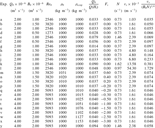
Range of experimental conditions. Here
 $Q_{0}$
(
 $\text{m}^{3}~\text{s}^{-1}$
) denotes the source volume flux, while
 $B_{0}$
(
 $\text{m}^{4}~\text{s}^{-3}$
) is the source buoyancy flux and
 $Re_{0}$
is the source Reynolds number. Density
 $\unicode[STIX]{x1D70C}_{0}$
(
 $\text{kg}~\text{m}^{-3}$
) is the density of the liquid phase at the plume source, while
 $\unicode[STIX]{x1D70C}_{a,top}$
(
 $\text{kg}~\text{m}^{-3}$
) is the density of the ambient fluid at the level of the plume source;
 $Q_{0}/Q(H_{t})$
is the ratio between the source volume flux and the volume flux at the top of the plume;
 $F_{s}$
is the fraction of the source buoyancy flux associated with the salinity of the source fluid;
 $N$
(
 $\text{s}^{-1}$
) is the Brunt–Väisälä buoyancy frequency; and
 $v_{s}$
(
 $\text{m}~\text{s}^{-1}$
) is the particle settling velocity. In all experiments, the density of the silicon carbide particles was
 $\unicode[STIX]{x1D70C}_{part}=3210~\text{kg}~\text{m}^{-3}$
.

3 Results of experiments
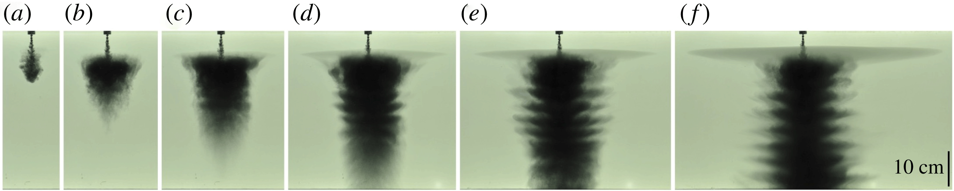
Figure 2 shows a series of photographs taken during a typical experiment (experiment e, see table 1). On entering the tank, the particle-laden fluid formed a descending turbulent plume (figure 2
a). For buoyancy fluxes of order
 $B_{0}\approx 10^{-6}~\text{m}^{4}~\text{s}^{-3}$
(see table 1), the downward speed of the plume fluid was of order
 $10^{-1}~\text{m}~\text{s}^{-1}$
above the neutral buoyancy height (Morton et al.
Reference Morton, Taylor and Turner1956). This greatly exceeds the particle fall speed
 $v_{s}$
except for experiment l (see table 1), and the particle plume behaved similarly to a single-phase plume in this region. The flow descended to the neutral buoyancy height, where it spread radially and the particles then gradually separated from the fluid forming a cylindrical column of sedimenting particles whose radius was independent of depth. In figure 2, the first radial intrusion is a little darker than the remaining ambient fluid owing to some very fine particles in the suspension which have a very small fall speed and essentially behave like a passive tracer. The first laterally spreading intrusion reached the walls of the tank after a time of order 1000 s. Most of our observations relate to earlier times in the evolution of the flow, so that the effects of filling-box processes do not control the dynamics (cf. Baines & Turner Reference Baines and Turner1969). Below the maximum height of the plume, an interesting, nearly regular pattern of small, finite intrusions developed at the edge of the descending column of particles (figure 2
d–f).
Photographs captured during experiment e (see table 1). Images captured at times (a) 6 s, (b) 24 s, (c) 50 s, (d) 90 s, (e) 138 s and (f) 338 s after the beginning of the experiment.

Motivated by these observations, a systematic series of experiments were run to measure: (i) the vertical distance from the source at which the fluid in the plume intruded once the particles had fallen out; (ii) the radius of the column of particles which descended below the neutral buoyancy level; (iii) the speed at which the particles descended below the first growing intrusion; and (iv) the properties of the regular series of small intrusions which form below the first main intrusion.
3.1 Intrusion of plume fluid
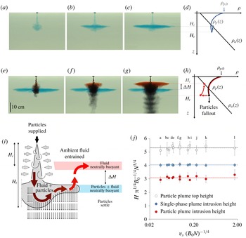
We first compare the behaviour of the fluid in a single-phase plume to that of the liquid phase in a particle plume. Figure 3 shows the results of two experiments, in which a single-phase plume and a particle plume with identical source buoyancy flux
 $B_{0}$
descended through the same ambient with a linear density stratification
 $N$
. In the single-phase experiment, a relatively dense saline solution with blue dye was supplied through the nozzle at the top of the tank (figure 3
a). This formed a plume which descended through the tank while entraining ambient fluid (figure 3
b). After reaching a maximum distance
 $H_{t}$
below the source, the plume fluid ascended towards the neutral buoyancy level, and formed a radial intrusion at a vertical distance
 $H_{i}$
below the source (figure 3
c,d).
Intrusions of (a–d) a single-phase plume and (e–h) a multiphase plume with identical
 $B_{0}$
(experiment i in table 1). (i) Schematic illustrating the flow dynamics. (j) Experimental measurements of the top and intrusion heights of single- and multiphase plumes (experiments a–l in table 1).

In the particle plume experiment, a suspension of heavy particles in fresh water was supplied through the same nozzle. Red dye was added to the water to observe its motion in the tank: the dye did not affect the density of the water, which had the same density as the ambient fluid at the top of the tank, so that
 $B_{s}=0$
(cf. table 1, experiment i). Figure 3(e) shows that at the beginning of the experiment, the particle-laden fluid descended to a similar maximum distance below the source as that reached by the single-phase plume. The particle-laden fluid then ascended to the same height at which the single-phase plume had formed the blue intrusion. At this height, the bulk density of the plume fluid was equal to that of the surrounding ambient fluid; however, the plume contained a mixture of heavy particles and relatively buoyant fluid. As the particles gradually separated from the flow and settled, the bulk density of the red particle-laden fluid decreased and the red fluid moved upwards towards a new level of neutral buoyancy in the upper part of the tank (figure 3
f), where it formed an intrusion. The distance
 $\unicode[STIX]{x0394}H$
between the blue and red intrusions is associated with the change in the density of the plume fluid caused by particle sedimentation (figure 3
g,h; experiment i in table 1).
Figure 3(j) illustrates the depth of the blue and the red intrusions formed by the single-phase plume and the particle plume for the series of experiments (a–l) listed in table 1. In these experiments, the density of the liquid phase supplied at the plume source was equal to that of the ambient fluid at the top of the tank,
 $B_{s}=0$
(see (2.1)). Hence, the source buoyancy flux was entirely the result of the particles in the source fluid,
 $B_{0}=B_{p}$
(see (2.2) and (2.3)). As may be seen in figure 3(j), the top heights of the plumes as measured in the experiments agree, within an error 6 %, with the original results of Morton et al. (Reference Morton, Taylor and Turner1956) for the height of a turbulent buoyant plume:
 $$\begin{eqnarray}H_{t}=5\unicode[STIX]{x03C0}^{-1/4}B_{0}^{1/4}N^{-3/4}.\end{eqnarray}$$
The salt plumes then intrude at a height
 $H_{i}=(0.80\pm 0.01)H_{t}$
while the particle plumes form an intrusion at a height
 $(0.58\pm 0.03)H_{t}$
.
In comparing the height of the plume with the classical model of Morton et al. (Reference Morton, Taylor and Turner1956), we should include a correction to the model prediction associated with the relatively high source momentum flux relative to that in a pure plume. This is typically achieved by including a virtual origin (Hunt & Kaye Reference Hunt and Kaye2001). In the present problem, owing to the design of the nozzle, which ensures the flow rapidly becomes turbulent, we estimate that this virtual origin is of order 0.6 cm. This estimate was validated based on the results of a reference filling-box experiment, in which single-phase saline fluid was supplied through the nozzle into an unstratified layer of fluid and the rate of ascent of the dense fluid in the ambient was measured at each height to determine the volume flux in the plume at each height (cf. Linden, Lane-Serff & Smeed Reference Linden, Lane-Serff and Smeed1990, Mingotti & Woods Reference Mingotti and Woods2015). Given the descent height of the plumes is of order 10–20 cm, the correction associated with the virtual origin suggests that the experimental plumes may extend a distance of 3–6 % beyond the prediction of the model, consistent with the variation in the experimental data.
If we assume that all particles sediment from the flow, then for
 $B_{s}=0$
the height of the resulting intrusion formed by the particle plume is associated only with the net buoyancy of the entrained fluid. As a simplified model, we now calculate the buoyancy at the maximum height of the plume according to classical plume theory, and we then compare the depth of ambient fluid with this buoyancy with the actual intrusion height. From classical plume theory, we calculate that the buoyancy of the entrained fluid relative to the ambient fluid at the source is given by
 $$\begin{eqnarray}g_{e}^{\prime }(z)=\frac{1}{Q(z)}\int _{0}^{z}g_{a}^{\prime }(\unicode[STIX]{x1D701})\frac{\text{d}Q}{\text{d}\unicode[STIX]{x1D701}}\,\text{d}\unicode[STIX]{x1D701},\end{eqnarray}$$
where
 $Q$
is the volume flux in the plume while the buoyancy of the ambient fluid at depth
 $z$
relative to the ambient fluid at the source,
 $z=0$
, is given by
 $g_{a}^{\prime }(z)=N^{2}z$
. To proceed, we solve the classical plume equations for the mass flux
 $Q(z)=\unicode[STIX]{x03C0}q(z)$
, momentum flux
 $M(z)=\unicode[STIX]{x03C0}m(z)$
and buoyancy flux
 $B(z)=\unicode[STIX]{x03C0}b(z)$
integrated across each horizontal plane (cf. Turner Reference Turner1973):
 $$\begin{eqnarray}\frac{\text{d}q}{\text{d}z}=2\unicode[STIX]{x1D6FC}m^{1/2};\quad \frac{\text{d}m}{\text{d}z}=bq/m;\quad \frac{\text{d}b}{\text{d}z}=-N^{2}q,\end{eqnarray}$$
where the entrainment coefficient
 $\unicode[STIX]{x1D6FC}$
is taken to have value
 $0.13$
for consistency with (3.1) for the total height of the plume. These equations are solved using a simple finite difference numerical scheme, with a sufficiently small step size to ensure convergence of the model predictions. The model equations are scaled using the source buoyancy flux
 $B_{0}$
and the frequency of the ambient stratification
 $N$
, following the approach of Morton et al. (Reference Morton, Taylor and Turner1956), and we assume that the dimensionless source mass and momentum fluxes are small so that the results are asymptotically correct for a so-called pure plume in which there is only a source of buoyancy. As mentioned above, the finite initial momentum flux in the experiments introduces an error of order 3–6 %, which we can represent in terms of a virtual origin so that the theoretical location of the source as used in the model calculations is 0.6 cm ahead of the actual experimental source.
Using the numerical solution for
 $q(z)$
, we find that at the plume top,
 $z=H_{t}$
, the buoyancy associated with the entrained fluid corresponds to ambient fluid at a height
 $2.9(B_{o}/\unicode[STIX]{x03C0})^{1/4}N^{-3/4}=0.58H_{t}$
below the source, while the total buoyancy corresponds to ambient fluid at a height
 $4.0(B_{o}/\unicode[STIX]{x03C0})^{1/4}N^{-3/4}=0.8H_{t}$
below the source. These predictions are consistent with the experimental data for the maximum height (white circles, equation (3.1)) and the height of the centre of the intrusions produced by the particle plumes (red circles,
 $z/H_{t}=0.58\pm 0.03$
) and the saline plumes (blue circles,
 $z/H_{t}=0.80\pm 0.01$
), as shown in figure 3(j).
As an aside, it is interesting to note that in the region between the plume source and the neutral buoyancy height, the model predicts that the volume flux in the plume increases at a rate almost equal to that of a plume in an unstratified environment (cf. Turner Reference Turner1973). This is a valuable observation, since in an unstratified environment, the plume equations admit similarity solutions in terms of the source buoyancy flux and the distance from the source. We now combine (3.2) with the similarity solution for the volume flux in an unstratified environment, which is given by Turner (Reference Turner1973),
 $Q(z)=\unicode[STIX]{x1D706}B_{o}^{1/3}z^{5/3}$
, where
 $\unicode[STIX]{x1D706}=(6/5)\unicode[STIX]{x1D6FC}\unicode[STIX]{x03C0}^{2/3}(9/10\unicode[STIX]{x1D6FC})^{1/3}$
is a constant. We then obtain the result that in an ideal plume with finite buoyancy flux and zero mass and momentum fluxes at the source, the buoyancy of the entrained fluid at a point
 $z$
between the source and the neutral buoyancy height is approximately equal to that of the ambient fluid at a height
 $5z/8=0.625z$
. The reason that the ultimate particle plume intrusion is predicted to occur at a lower height
 $0.58H_{t}$
rather than
 $0.625H_{t}$
is, in part, a result of the reduction in the rate of entrainment between the neutral height and the plume top, as the flow speed falls to zero and the motion diverges from the self-similar regime. We note that an indication of the smaller intrusion height of a multiphase plume has been seen in some earlier experiments: Seol et al. (Reference Seol, Bryant and Socolofsky2009) in fact presented data showing that the ratio of the intrusion or trap height to the top or peel height of the plume has values in the approximate range
 $0.55\pm 0.05$
(see their figure 4a). However, they did not present a quantitative model, based on classical plume theory, to explain this result as illustrated above. We note also that in their experiments of discrete particle-laden thermal clouds, Bush et al. (Reference Bush, Thurber and Blanchette2003) presented a similar approximate calculation to estimate the density of the particle-free fluid in the thermal at the maximum height of the thermal, leading to the prediction that, once the particles have separated from the flow, the fluid has a neutral buoyancy height equal to 0.75 of the total plume height. This quantitative difference from our prediction for a plume arises from the different rate of entrainment of ambient fluid into a plume and a thermal.
3.2 Effect of buoyancy of the source fluid
In the above analysis we explored the effect of particle–fluid separation on the final intrusion depth of the fluid carried by the plume. This revealed that the buoyancy of the particle-laden plume fluid at the maximum depth of the plume is comparable to that of the ambient fluid at a height of 0.8 of this maximum depth. Also, the net buoyancy of the source fluid constitutes a fraction of about 22/80 of the final buoyancy of the plume fluid, where the buoyancy is measured relative to the ambient fluid at the depth of the source, while the buoyancy of the entrained fluid represents the remaining fraction 58/80 of the final buoyancy of the plume fluid at the maximum depth. When the buoyancy of the source fluid arises from the presence of particles which can separate from the intrusion, then after the separation, the remaining buoyancy therefore leads to an intrusion at a depth of about 0.58 of the maximum depth of the plume.
However, if the buoyancy flux of the source fluid is composed of a component associated with the particle flux,
 $B_{p}$
, and a component associated with the source fluid,
 $B_{s}$
, then as the particles separate from the intrusion, the fraction
 $F_{s}=B_{s}/(B_{p}+B_{s})$
of the source buoyancy flux remains in the intrusion. As a result, in this case we would expect the final depth of the intrusion to be
 $$\begin{eqnarray}H_{i}=(0.58+0.22F_{s}\pm 0.03)H_{t},\end{eqnarray}$$
where
 $H_{t}$
is the maximum depth of the plume. In order to test this model, and explore the range of intrusion depths as the buoyancy of the source fluid changes, we have varied
 $F_{s}$
from the value
 $F_{s}=-0.58/0.22=-2.64$
for which the intrusion should have zero depth to the value
 $F_{s}=1$
for which the plume is purely composed of saline fluid and the intrusion has depth 0.8 of the maximum plume depth, corresponding to the case originally described by Morton et al. (Reference Morton, Taylor and Turner1956) (
 $B_{0}=B_{s}$
, see blue dots in figure 3
j).
In the experiments, this range of behaviour was achieved either by using very saline source fluid and a small flux of particles to model the cases with
 $F_{s}>0$
(experiments m–o in table 1) or by using a density stratification in the ambient fluid in which the fluid at the top of the stratified layer was saline while the particle-laden input fluid was fresh, to model the situation in which
 $F_{s}<0$
(experiments p–x in table 1). By using a large contrast in salinity between the fluid at the top of the stratified layer and the input fluid, the volume flux of source fluid could be kept to relatively small values compared to the volume flux at the maximum depth of the plume (
 $Q_{0}/Q(H_{t})\ll 1$
, see table 1), while the total buoyancy flux of the plume, and hence the maximum depth of the plume, was fixed. This ensured that, at the maximum depth of the plume, the source volume flux did not influence the averaged buoyancy associated with the fluid entrained into the plume, and hence (3.4) should apply.
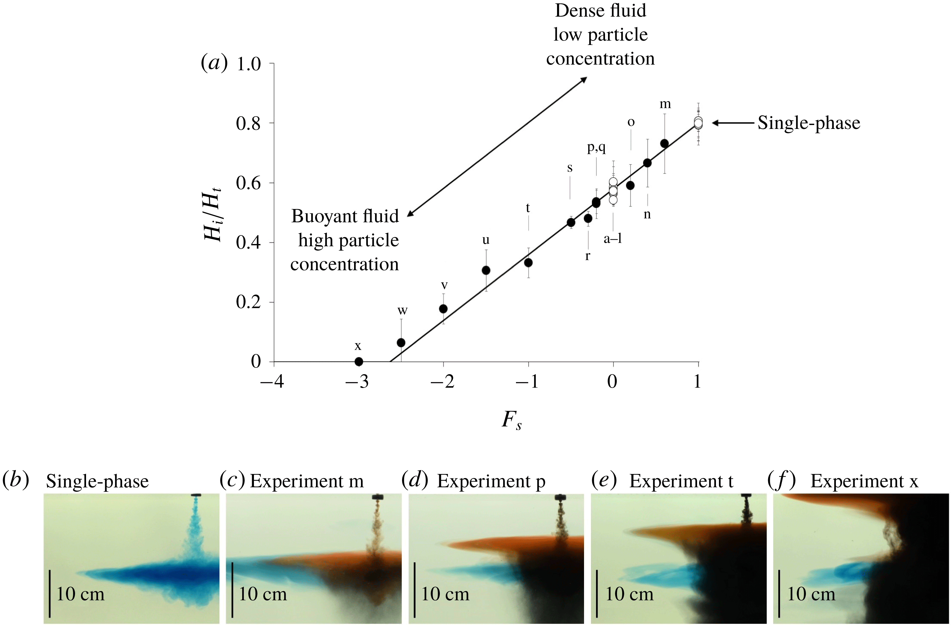
(a) Intrusion of saline particle-laden plumes descending through a stratified ambient (experiments m–x in table 1). (b–f) Photographs captured during experiments m, p, t and x (see table 1). Each photograph shows the final depth of the particle plume intrusion (red dye), and compares it with that of a single-phase plume with identical buoyancy flux
 $B_{0}$
(blue dye).

In figure 4(a) we present a series of experimental results showing the depth of the final intrusion as a fraction of the total depth of the plume for several values of
 $F_{s}$
, ranging from
 $-3.0$
to
 $1.0$
. It is seen that the data follow the model prediction (equation (3.4) above) with reasonable accuracy over the full range of values of
 $F_{s}$
. In figure 4(b–f) we also present a series of photographs of the final intrusion, compared to the intrusion of the equivalent single-phase plume, for the values
 $F_{s}=0.6$
(experiment m),
 $F_{s}=-0.2$
(experiment p),
 $F_{s}=-1.0$
(experiment t) and
 $F_{s}=-3.0$
(experiment x). All these data are shown in figure 4(a), as well as the results of the other experiments listed in table 1.
This analysis and our new experiments have important implications for the final intrusion height of fluid carried in a two-phase plume through a stratified fluid. If material on the particles dissolves into the water, knowledge of the intrusion height may be especially important for managing the environmental impact of the plume (see § 6).
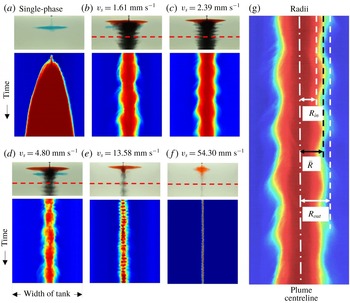
(a) Transient diameter of a single-phase plume intrusion. (b–f) Transient diameters of the column of descending particles in multiphase plumes (experiments c, e, i, k and l in table 1). (g) Inner radius
 $R_{in}$
(m), time-averaged mean radius
 $\bar{R}$
(m) and outer radius
 $R_{out}$
(m) of the particle column.

4 Column of descending particles
We now focus on the column of descending particles which is formed below the intrusion (see figure 2). Figure 5 illustrates how the diameter of this column changed over time in a number of different experiments. Each panel in the figure shows a time series of a horizontal line of pixels, in false colour, as recorded by a digital camera. The line is located at a depth 28 cm below the source (red dashed lines in figure 5
b–f). The diameter of an intrusion as a function of time produced by a single-phase plume is plotted in figure 5(a) for comparison. It is seen that the radius of this single-phase intrusion grows with time and eventually reaches the vertical walls of the tank. Conversely, the column of particles generated by each multiphase plume converges to a quasi-steady state, at which its radius oscillates around a mean value
 $\bar{R}$
(m). Figure 5(b–f) shows that
 $\bar{R}$
decreases when the particle settling speed
 $v_{s}$
is increased. In figure 5(g) we illustrate how the inner,
 $R_{in}$
, the mean,
 $\bar{R}$
, and the outer radius of the descending cylinder,
 $R_{out}$
, vary in time in a typical experiment (experiment e in table 1).
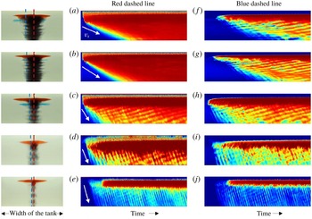
Time series of two vertical lines of pixels in false colour: (a–e) along the plume axis (red dashed line) and (f–j) at the edge of the cylinder (blue dashed line). The experiments shown in these images correspond to experiments c, e, i, j and k in table 1.

In figure 6 we compare the different speeds at which the particles descended towards the base of the tank in a number of experiments. Figure 6(a) shows a time series of a vertical line of pixels, in false colour, located along the plume centreline, as recorded by a digital camera in experiment c (see table 1). It is seen that before the beginning of the experiment, the tank did not contain any particles (blue colour on the left-hand side of figure 6
a). At the beginning of the experiment, the particle-laden flow formed a plume which rapidly descended from the nozzle towards the neutral buoyancy level: this is illustrated by the red front with a steep gradient in the upper left corner of figure 6(a). In the lower portion of the tank, however, the particles did not descend at the convective plume speed: instead, they fell more slowly at their Stokes settling velocity
 $v_{s}$
(see white arrow in figure 6
a). Figure 6(b–e) illustrates the results of a series of experiments each using particles of a different fixed size. In all of these experiments, the mean speed of the particles descending to the base of the tank was determined from the downward-pointing streak lines in figure 6. These speeds were found to be equal to the settling velocity
 $v_{s}$
, with fluctuations of less than 5 %. We note that for experiment l, in which the particle speed matches the plume speed above the neutral height, there is no lateral intrusion of the particle–fluid mixture. Instead, as the plume speed decreases to values smaller than the fall speed of the particles, the particles separate to form a narrow cylindrical column through which they sediment to the base of the tank, and the plume fluid rises back towards its neutral height.
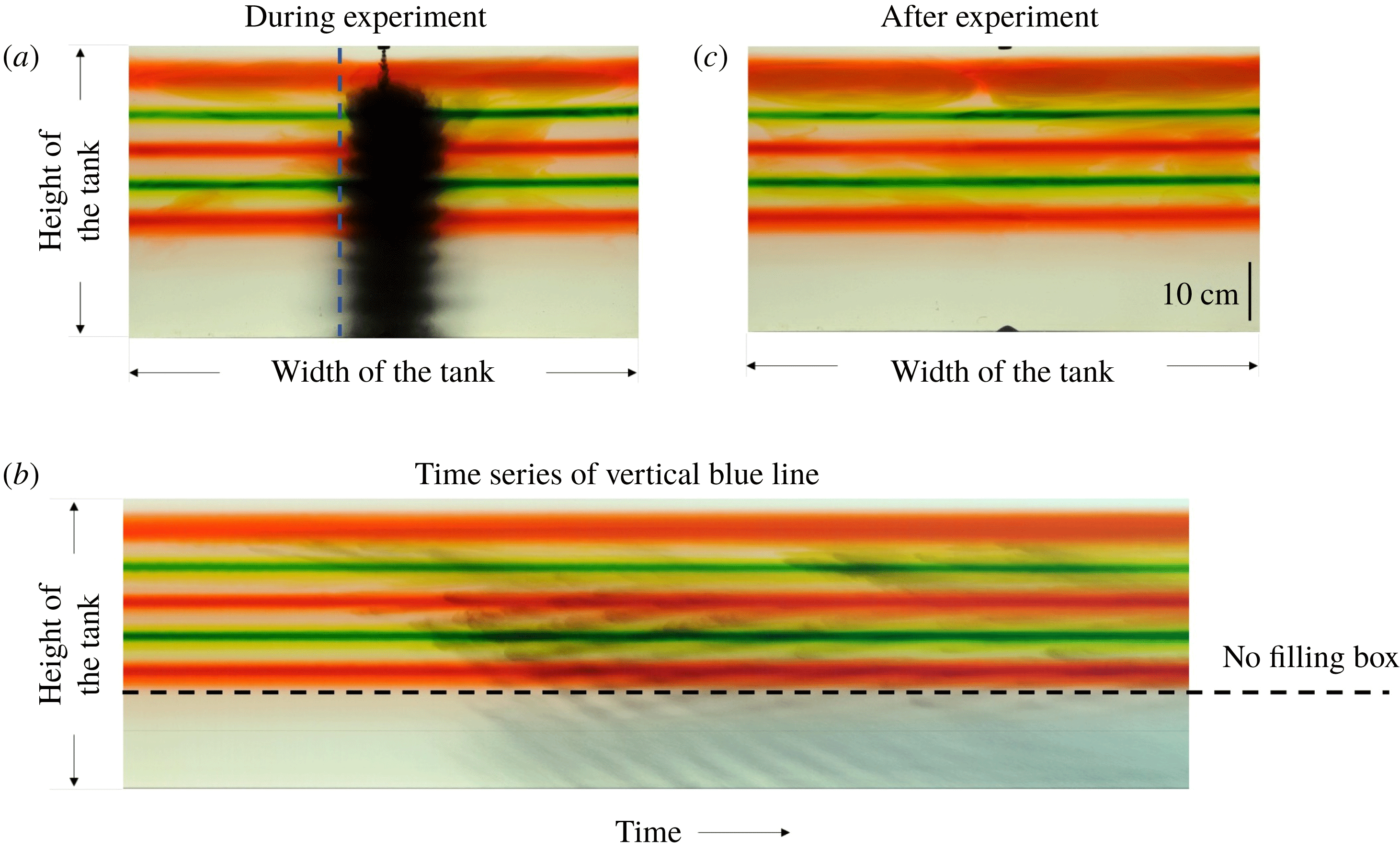
To investigate whether any fluid was transported towards the base of the tank by the settling particles, we added a few layers of dye which extended horizontally across the whole of the ambient fluid in the upper part of the tank in some of our experiments. We then observed the motion of the dyed fluid during each experiment. If the plume of particles convects fluid downwards through the tank, we would expect a return flow in the ambient fluid, and the layers of dye would slowly ascend. Figure 7 illustrates the outcome of experiment f (see table 1). The image in figure 7(a) was captured during the experiment. It is seen that the upper part of the tank contained five layers of dyed fluid (three red layers and two green layers), while the lower part of the tank was clear. The particle-laden plume just below the source, and the descending cylinder of particles deeper in the tank can be seen in this image. Figure 7(b) shows the time series of the vertical line of pixels indicated by the dotted blue line in figure 7(a). In this panel, a series of grey lines which are inclined downwards with time may be seen, and these correspond to the downward motion of particles through the tank. Figure 7(b) also indicates that some localised mixing of the dyed fluid occurred in the upper part of the tank during each experiment. However, the horizontal planes of dye do not seem to move vertically during the experiment, suggesting that fluid was not transported either (i) to the base of the tank by the cylindrical column of sedimenting particles or (ii) back upwards as a return flow in the ambient, to balance any downward fluid motion which may accompany the descending particles. Indeed, an image taken after all the particles had sedimented shows there is no dye in the fluid at the base of the tank and the layers of dye appear largely undisturbed (see figure 7 c). The very upper dye layer, which is located in the region of the initial descending turbulent plume, does show a small upward displacement, but this is small owing to the small plume volume flux near the source.
Horizontal layers of dyed fluid are added to the ambient (experiment f, see table 1).

These experimental observations suggest that for
 $z>H_{t}$
the multiphase plume transitions into a column of individually settling particles, and that there is no net vertical transport of the ambient fluid in the tank. This result may seem rather counterintuitive, because owing to the presence of the particles, the bulk density of a parcel of fluid in the column exceeds that of the surrounding ambient. To rationalise why no large-scale vertical convection of the particle-laden fluid occurs, we first quantify the radius
 $R$
of the column of settling particles, and the mean concentration of particles in the column,
 $C_{c}$
. At steady state, conservation of mass requires that the flux of particles settling through the cross-sectional area of the column equals the flux of particles supplied at the source:
 $$\begin{eqnarray}Q_{0}C_{0}=\unicode[STIX]{x03C0}R^{2}v_{s}C_{c},\end{eqnarray}$$
in which
 $Q_{0}$
(
 $\text{m}^{3}~\text{s}^{-1}$
) is the source volume flux and
 $C_{0}$
is the source concentration. The mean concentration of particles in the plume at a distance
 $z=H_{t}$
below the source is given by
 $$\begin{eqnarray}C_{c}=\frac{Q_{0}}{Q(H_{t})}C_{0}.\end{eqnarray}$$
By solving the plume equations (3.3), we predict that the volume flux at
 $z=H_{t}$
is
 $Q(H_{t})=0.96\unicode[STIX]{x03C0}^{1/4}B_{0}^{3/4}N^{-5/4}$
, and combining this with (4.1) and (4.2) we predict that the radius of the column will then follow the law
 $$\begin{eqnarray}R=k_{1}B_{0}^{3/8}N^{-5/8}v_{s}^{-1/2},\end{eqnarray}$$
where
 $k_{1}=0.64$
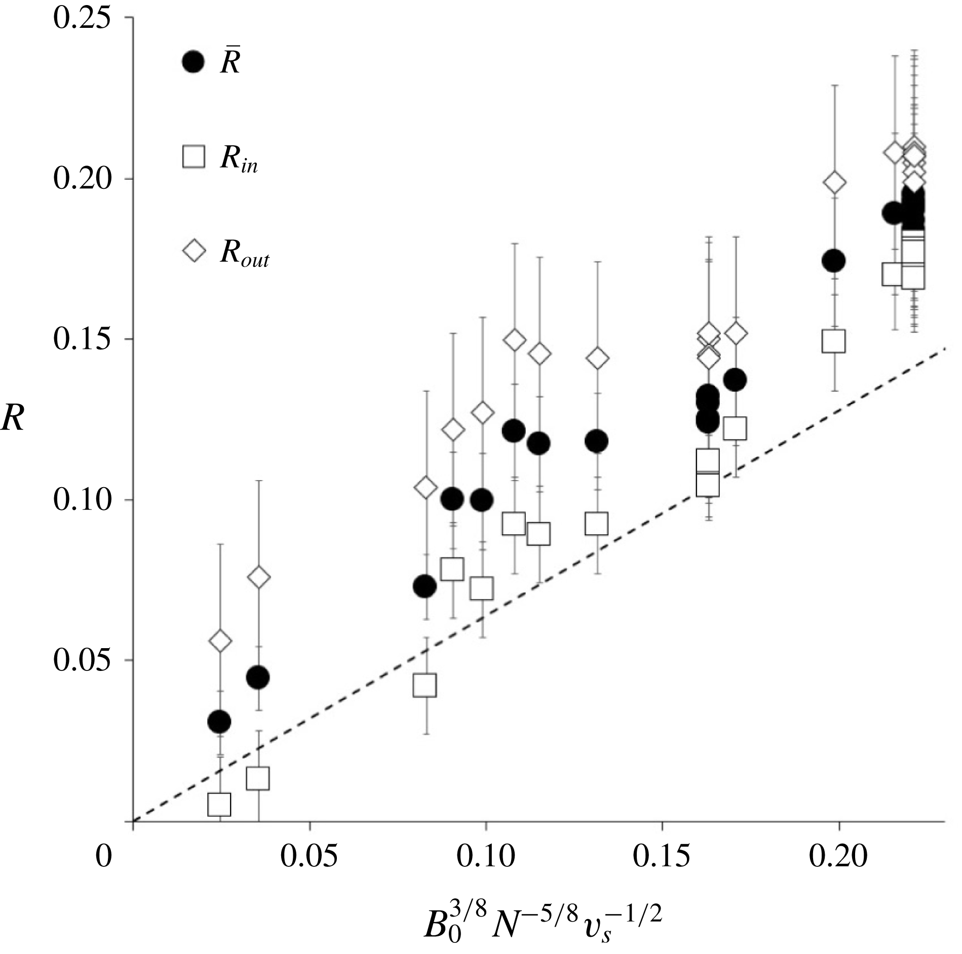
. Figure 8 shows that the data follow a linear trend of the form suggested by (4.3), but the constant of proportionality for the mean radius
 $\bar{R}$
is about 25 % larger than the model prediction (solid circles in figure 8). This difference is associated with the lateral intrusions seen on the edge of the particle-laden column. It is seen that there is a closer agreement between the prediction of the model and the inner radius
 $R_{in}$
(white squares in figure 8; cf. figure 5
g), with errors of order 5–7 %. We note that Chan et al. (Reference Chan, Chow and Adams2015) introduced a similar scaling by calculating the radius to which particles in the initial plume intrusion spread before sedimenting into the underlying fluid. However, they did not present data on the descending column of particles, but instead related this radius to that of the ultimate sediment deposit on the base of the tank.


Using (4.1) and (4.3), we calculate that the reduced gravity of a parcel of particle-laden fluid in the column relative to the surrounding ambient,
 $g_{c}^{\prime }$
(
 $\text{m}~\text{s}^{-2}$
), is given by
 $$\begin{eqnarray}g_{c}^{\prime }=\frac{B_{p}}{Q(H_{t})}=\unicode[STIX]{x03C0}^{-1}k_{1}^{-2}(1-F_{s})B_{0}^{1/4}N^{5/4}.\end{eqnarray}$$
Using (4.4), we estimate that the maximum distance
 $\unicode[STIX]{x0394}z$
that a parcel of particle-laden fluid could travel before reaching the level at which its density matches the density of the ambient fluid is given by
 $$\begin{eqnarray}\unicode[STIX]{x0394}z=\frac{g_{c}^{\prime }}{N^{2}}=\unicode[STIX]{x03C0}^{-1}k_{1}^{-2}(1-F_{s})B_{0}^{1/4}N^{-3/4}.\end{eqnarray}$$
By combining equations (4.3) and (4.5) we obtain the ratio between
 $\unicode[STIX]{x0394}z$
and
 $R$
:
 $$\begin{eqnarray}\frac{\unicode[STIX]{x0394}z}{R}=\frac{1}{\unicode[STIX]{x03C0}k_{1}^{3}}(1-F_{s})\left(\frac{v_{s}}{B_{0}^{1/4}N^{1/4}}\right)^{1/2}.\end{eqnarray}$$
Equation (4.6) suggests that in the situation we are modelling, in which the particle fall speed
 $v_{s}$
is less than the characteristic speed of the plume,
 $(B_{0}N)^{1/4}$
, then the maximum distance that a parcel of particle-laden fluid can travel by convection,
 $\unicode[STIX]{x0394}z$
, is smaller than the radius of the column,
 $R$
, and so steady downward convection of the particle-laden fluid in the column is suppressed.
5 Particle layers and fluid recirculation in the column
Although the data and arguments presented in § 4 suggest that there is no vertical transport of fluid in the column, in § 3 we observed that a series of small intrusions develop at the edge of the cylindrical column through which the particles sediment (figure 2). We also noted that these small intrusions seem to be associated with regular oscillations in the radius of the particle column over time (figure 5). Also, a series of horizontal layers with higher and lower particle concentration seem to rise slowly through the column, as suggested by the upward-sloping lines which may be seen in the time-series images plotted in figure 6(f–h). Nonetheless, the scaling for the column radius (equation (4.3) and figure 8) suggests that the overall control on the particle descent through the column is the settling speed of the particles. In this section, we explore the character of these layers and oscillations in further detail. For convenience we focus on our experiments in which
 $B_{s}=0$
, and the plume is driven by a source of dense particles.
(a–e) Series of photographs captured during experiment y (see table 1). The time lapse between these photographs was 22.8 s. In this experiment, glass beads of a mean settling speed
 $v_{s}=2.38\times 10^{-3}~\text{m}~\text{s}^{-1}$
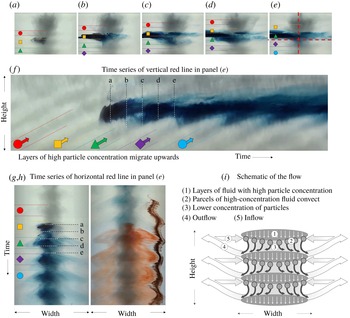
were supplied at the plume source, and formed a semi-transparent cylinder. A blob of neutrally buoyant blue dye was squirted into the cylinder to observe the motion of the fluid within the column of settling particles. Coloured symbols are used in the figure to identify five successive layers of particle-rich fluid as they migrate upwards along the cylinder. (f) A time series of the vertical line of pixels indicated by the dashed vertical red line in (e) is shown. The different times at which photographs a–e were captured during the experiment are identified within this image. Coloured symbols are used to identify the layers of particle-rich fluid depicted in (a–e). (g,h) Time series of the horizontal line of pixels indicated by the dashed horizontal red line in (e). Coloured symbols are used to identify the time intervals during which the layers of high particle concentration pass through the horizon. (i) Schematic illustrating the motion of the particles and of the fluid in the system.

In figure 9(a–e), we present a series of images of the time evolution of the column of particles after a parcel of neutrally buoyant blue dye has been injected into the core of the column. It is seen that over the course of more than 80 s, the blue dye moves laterally outwards, but there is relatively little vertical motion of the dye in the tank, a result which is consistent with the stationary planes of dyed fluid described earlier (figure 7). In figure 9(f) we present a time series of a vertical line of pixels through the column. Here, a series of diagonal grey bands may be seen, which correspond to layers of particle-rich fluid in the column (cf. figure 9
i,
 $\unicode[STIX]{x2460}$
). Over time, these layers ascend through the tank, as denoted by the red, yellow, green, purple and blue arrows depicted in figure 9(f). The particles in each of these layers gradually settle towards the bottom of the layer (cf. white arrows in figure 9
i). On the lower surface of each particle-rich layer, small parcels of high-concentration particle-laden fluid sink into the lower-concentration fluid below (cf. figure 9
i,
 $\unicode[STIX]{x2461}$
–
 $\unicode[STIX]{x2462}$
). These parcels appear as the downward-sloping dark lines emanating from the lower surface of the grey bands in figure 9(f). As the parcels descend through the stratified fluid, they gradually decelerate. This causes the particles to separate from the fluid and settle out of each parcel into the next layer of particle-rich fluid below. As a result of particle separation, the fluid in each parcel becomes relatively buoyant and begins to spread radially outwards and upwards. Eventually, the fluid rises back to its neutral buoyancy height (cf. figure 9
i,
 $\unicode[STIX]{x2463}$
). During the time required for the fluid in the parcel to descend from the bottom of one layer, separate from the particles and rise back up towards its neutral buoyancy level, the whole series of particle-rich layers in the column gradually migrates upwards. This happens because the convective parcels of descending fluid continuously remove particles from the bottom of each layer and deposit them onto the top of the layer below, causing the centre of mass of the layers to rise slowly over time. On the lower part of each particle-rich layer, there appears to be a slow inflow towards the centre of the cylinder replacing the flux of fluid moving down in the particle-laden parcels (cf. figure 9
i,
 $\unicode[STIX]{x2464}$
). If the time required for a parcel of particle-laden fluid to descend, lose its particle content, spread radially outwards as it rises back to the neutral height and then flow back in towards the cylindrical region matches the time required for the particle layer to rise a distance equal to the spacing between the layers, then a series of regular convective recirculation cells may develop. Each cell will fill the region between a particle-rich layer and the one below, as sketched in figure 9(i).
Such periodic recirculation of the fluid in the system is illustrated by the displacement of the blue dye in figure 9(f). Here, we observe that the layer denoted by the yellow square symbol contains the dyed fluid initially (see figure 9 a,b). A series of parcels of particle-laden dyed fluid then descend from this layer to the next one (denoted by the green triangle, see figure 9 b,c). The dyed fluid then slowly ascends as the layer denoted by the green symbol gradually rises through the system (figure 9 d,e). On reaching the height at which it was originally injected, the dyed fluid is drawn back into the centre of the column, where it is supplied with sedimenting particles, and then carried downwards with further particle-laden parcels of convective fluid, which descend to the next particle-rich layer (denoted using a purple diamond). At this point, the cycle repeats, and the fluid undergoes a slow rise followed by a rapid descent (figure 9 f).
To complement these images, in figure 9(g,h) we present time series of two horizontal lines through the same flow. In figure 9(g), the same coloured symbols as in figure 9(a–f) are used to illustrate when the different particle-rich layers rise through the window of observation. Figure 9(g,h) shows a series of radially inward and outward motions, as part of the net convective recirculation of the fluid associated with the particle fallout. On the right-hand side of figure 9(h), we can see the time evolution of the point of intersection of a vertical line of brown tracer located just outside the cylinder with this horizontal line of pixels. This illustrates that there is a regular cycle of inflow and outflow.
We now develop a model which quantifies the vertical distance between the layers of particle-rich fluid,
 $\unicode[STIX]{x1D6FF}$
(m), and the mean speed,
 $u_{up}$
(
 $\text{m}~\text{s}^{-1}$
), at which these layers migrate upwards.
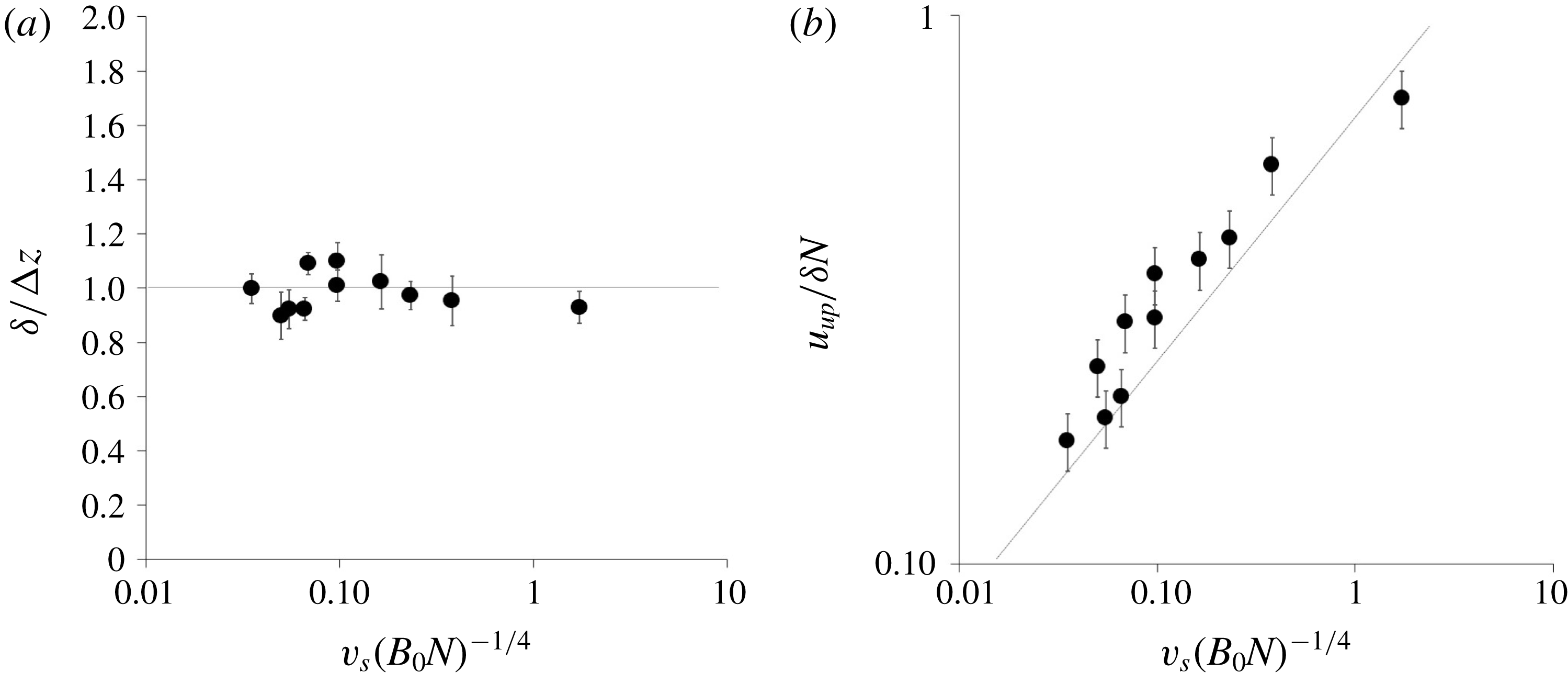
Time-averaged mean (a) spacing between the intrusions
 $\unicode[STIX]{x1D6FF}$
and (b) upward speed of the intrusions
 $u_{up}$
. The line in (b) corresponds to
 $u_{up}=0.05v_{s}^{1/2}(B_{0}N)^{1/8}$
. Data are plotted for experiments a–l in table 1.

From figures 6 and 9 it may be seen that the average vertical spacing between the layers of particle-rich fluid was approximately constant over the course of each of our experiments, with fluctuations of order 5–10 %. Given that the density difference between the column and the surrounding fluid is associated with the particle load, then we expect the spacing between the layers to be given by the balance of this density difference and the ambient density gradient (see (4.5)). Figure 10(a) shows that the spacing between the intrusions,
 $\unicode[STIX]{x1D6FF}$
, measured from images of the experiments, is indeed controlled by this ratio of the buoyancy of the particle cloud and the background stratification, as given by (4.5). We note that this spacing is similar to the spacing of the intrusions seen in stratified Boycott-effect experiments (Peacock, Blanchette & Bush Reference Peacock, Blanchette and Bush2005).
In order to determine the upward speed of the particle-rich layers of fluid,
 $u_{up}$
(
 $\text{m}~\text{s}^{-1}$
), we equate the time of ascent of the layers through a distance
 $\unicode[STIX]{x0394}z$
,
 $$\begin{eqnarray}\unicode[STIX]{x1D70F}_{up}=\frac{\unicode[STIX]{x0394}z}{u_{up}},\end{eqnarray}$$
with the time required for a parcel of particle-laden fluid to descend vertically from the bottom of one of the layers, sediment its particles and spread laterally outwards while rising back upwards to its original height (figure 9
i). Figure 9(f) suggests that this latter recirculation is slower than the initial convective descent of the parcel, and hence that the recirculation time regulates the upward speed of the layers. The time scale for the recirculation is given by the ratio of the radius of the column,
 $R$
(see (4.3)), and the speed of the lateral intrusion,
 $u_{in}$
(
 $\text{m}~\text{s}^{-1}$
). The intrusion is driven by the release of buoyant fluid following the sedimentation process, and so we expect
 $u_{in}$
to scale as
 $(g_{c}^{\prime }\unicode[STIX]{x0394}z)^{1/2}$
. Using the expression for
 $\unicode[STIX]{x0394}z$
given in (4.5), the intrusion speed can then be written as
 $$\begin{eqnarray}u_{in}=k_{2}\frac{g_{c}^{\prime }}{N}=k_{3}B_{0}^{1/4}N^{1/4},\end{eqnarray}$$
where
 $k_{2}$
and
 $k_{3}=\unicode[STIX]{x03C0}^{-1}k_{1}^{-2}k_{2}$
are two constants. Hence, the time for the recirculation of the fluid,
 $\unicode[STIX]{x1D70F}_{r}$
(s), scales as
 $$\begin{eqnarray}\unicode[STIX]{x1D70F}_{r}=k_{4}N^{-1}(B_{0}N)^{1/8}v_{s}^{-1/2},\end{eqnarray}$$
where
 $k_{4}=k_{1}/k_{3}$
is a constant. By setting
 $\unicode[STIX]{x1D70F}_{up}=\unicode[STIX]{x1D70F}_{r}$
, we predict that the upward speed of migration of the particle-rich layers follows the scaling
 $$\begin{eqnarray}u_{up}=k_{5}(v_{s}(B_{0}N)^{1/4})^{1/2},\end{eqnarray}$$
where
 $k_{5}$
is a constant. In figure 10(b) we compare the upward speed of the layers as measured in the experiments with this scaling law, shown by the solid line, and we find reasonable agreement. In fact, from figure 10(b) we deduce that
 $k_{5}=0.05$
and the upward speed of the particle-rich layers is consistent with
 $u_{up}=0.05v_{s}^{1/2}(B_{0}N)^{1/8}$
.
6 Discussion
In this paper, we have explored the dynamics of dense particle plumes moving through a stratified fluid in the limit
 $v_{s}<(B_{0}N)^{1/4}$
. We have established that a turbulent particle plume descends to a maximum depth equal to that reached by a single-phase plume with the same source buoyancy flux. However, at this point, the particles begin to sediment from the flow, reducing the buoyancy of the remaining particle-free plume fluid. This fluid then rises to a depth given approximately by the fraction
 $0.58+0.22F_{s}\pm 0.03$
of the maximum plume depth, where it spreads out to form an intrusion. Here,
 $F_{s}$
denotes the fraction of the source buoyancy flux associated with the buoyancy of the source fluid relative to the ambient fluid at the top of the system, with the remainder being associated with the particle load. When
 $F_{s}=1$
, the plume intrusion depth corresponds to the prediction from classical plume theory of the depth at which the ambient fluid density equals the density of the plume fluid at the maximum height of the plume; however, if
 $F_{s}<1$
as in the case of particle plumes, the intrusion height is smaller, and for
 $F_{s}=-2.64$
, the fluid eventually intrudes at the injection level. We have shown that our prediction of the depth of the intrusion is consistent with the results of a systematic series of new laboratory experiments. Below the plume, the particles continue to sediment under their individual fall speed, within a cylindrical region whose radius depends on the fall speed, the particle load in the plume and the original particle flux. There is negligible vertical transport of ambient fluid below the plume. However, small intrusions form on the outer boundary of the cylindrical region of sedimenting particles. These intrusions have spacing given by the fraction
 $0.2k^{-2}\unicode[STIX]{x03C0}^{-3/4}$
of the plume height (equations (3.1) and (4.5)), and they slowly rise along the edge of the cylindrical region with speed
 $u_{up}\sim 0.05v_{s}^{1/2}(B_{0}N)^{1/8}$
. These intrusions primarily lead to lateral motion of the fluid rather than producing any significant vertical transport of fluid.
The experimental results have some key implications for large-scale environmental flows. First, in deep-sea mining applications, it is envisaged that particles scooped up from the sea floor are transported by a riser to a ship, where they are processed and the waste solid material may then be released back into the water at the surface. This will form a particle plume which descends through the stratified ocean water. On reaching its neutral height, the plume fluid will spread out and form an intrusion. The depth of this intrusion may differ significantly from that produced by a single-phase plume, which always spreads at a depth of approximately
 $0.80\pm 0.01$
of the maximum depth. Second, there is negligible large-scale vertical transport of ambient fluid below the plume, and so any contaminants which dissolve into the fluid below the plume will remain at that depth, but may spread laterally through the migrating intrusions as described in § 5. However, we recognise that ambient currents are likely to have an impact on this sedimenting column of particles, and although there has been some modelling, further research is required to develop a detailed quantitative understanding of how the intrusion process described herein interacts with a background flow (e.g. Socolofsky & Adams Reference Socolofsky and Adams2005).
We might expect similar behaviour in a bubble plume composed of bubbles whose rise speed is smaller than the characteristic speed of the plume. However, in bubble plumes with a range of bubble sizes, the larger bubbles may rise as a separate flow through the centre of the plume, while the smaller, more dispersed bubbles may continue rising as a plume, producing a more complex hybrid flow (cf. McDougall Reference McDougall1978). Beyond the plume, the particles or bubbles with different rise speed may lead to nested cylinders, with the fast-moving particles only appearing in the central core, while smaller particles migrate through a much larger cylinder. This can lead to complex intrusion and layering processes, and we plan to explore this in new experiments.
However, already with the present model, one can envisage calculating the intrusion height of water produced by a buoyant droplet plume rising from the sea floor following a blowout for example (cf. Socolofsky et al.
Reference Socolofsky, Adams and Sherwood2011). In a bubble or droplet plume, there may be a range of bubble sizes, and a more complex model may be needed to account for the fraction of the bubble population which moves with the flow, for which
 $u<(B_{0}N)^{1/4}$
, and that which rises relative to the flow, for which
 $u>(B_{0}N)^{1/4}$
. As we have shown, the prediction of the intrusion height is strongly dependent on the separation of the droplets from the initial intrusion and also depends on the density of the water in the plume at the source. For a pure oil or gas release on the sea floor, the density of the water in the source fluid may be similar to the density of the water at the sea floor. As this plume initially intrudes at its neutral buoyancy height, the oil and gas separates from the flow, and this leads to intrusion of the plume fluid at a lower height in the water column. With a linear stratification, the intrusion height would be about
 $0.58/0.8\sim 0.75$
of the intrusion height for a single-phase plume. However, if there is some geological water which issues from the reservoir with the oil and gas, this may have a density different from that of the water at the sea floor. As a result, after reaching the top height of the plume, the separation of the oil and gas could then lead to descent of the water to a different height in the water column, akin to the experiments shown in figure 4.