1 Introduction
1.1 General context: problems on time-dependent domains
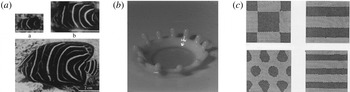
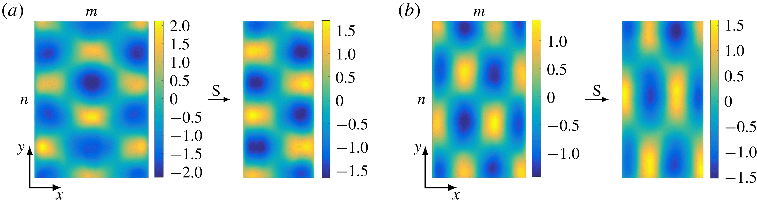
Patterns observed in problems on time varying domains: (a) Pomacanthus semicirculatus (Painter, Maini & Othmer Reference Painter, Maini and Othmer1999); (b) crown in the drop splash problem (Hartong-Redden & Krechetnikov Reference Hartong-Redden and Krechetnikov2011); (c) reaction–diffusion on a growing square domain (Madzvamuse, Maini & Wathen Reference Madzvamuse, Maini and Wathen2003).

Despite the ubiquity of physical systems evolving on time-dependent spatial domains ranging from crystal growth, skin patterns on tropical fish (figure 1 a) and crown in the drop splash problem (figure 1 b) to quantum particles travelling in a time-evolving potential and galaxy agglomeration in the expanding Universe, to name a few, understanding their dynamical properties is still in a rudimentary state (Knobloch & Krechetnikov Reference Knobloch and Krechetnikov2015). For example, standard boundary-value theory developed for ordinary and partial differential equations on time-fixed domains proves to be largely irrelevant because after mapping time-dependent onto time-fixed domains, the differential operators become non-autonomous, thus simply moving the difficulty to a different realm. Hence, advancing, both theoretically and experimentally, our understanding of the very basic elements in the dynamics on time-varying domains is vital for penetrating into the nature of more complex phenomena.
One area where many efforts have been recently put forth is developmental biology, providing both counterpart – reaction–diffusion versus fluid roll system – and context for our study. Historically, morphogenesis in biology – e.g. the stripe patterning observed in the aging Pomacanthus fish (Kondo & Asai Reference Kondo and Asai1995; Painter et al. Reference Painter, Maini and Othmer1999) – was originally suggested by Turing (Reference Turing1952) to be due to reacting and diffusing morphogens, which interact to produce, via an instability, patterns in concentration. The issue, however, is that this Turing instability on stationary domains occurs under quite restrictive diffusion-controlled conditions: namely, to achieve an instability one must enforce one of the species to diffuse much faster than the other, and hence, due to sensitivity, pattern formation requires tight control of involved parameters and initial conditions and therefore cannot be considered as robust. This constitutes one of the major criticisms of reaction–diffusion theory for pattern formation (Bard & Lauder Reference Bard and Lauder1974), although Turing-type patterns were eventually observed experimentally (Castets et al. Reference Castets, Dulos, Boissonade and Kepper1990; Ouyang & Swinney Reference Ouyang and Swinney1991). In the search for more robust pattern formation in reaction–diffusion systems, various modifications to the original Turing treatment have been made, in particular taking into account domain growth and changes in geometry (figure 1 c). Crampin, Gaffney & Maini (Reference Crampin, Gaffney and Maini1999) showed that in one dimension domain growth may be a mechanism for increased robustness, e.g. in the case of exponential growth a frequency-doubling sequence appears. In fact, there are examples of reaction–diffusion systems which cannot exhibit a diffusively driven instability on a fixed domain, but are unstable in the presence of slow domain growth (Madzvamuse, Gaffney & Maini Reference Madzvamuse, Gaffney and Maini2010). Despite much progress in observations, most of the above studies resort to numerical simulations, thus providing little insight into the fundamental underlying mechanisms responsible not only for various metamorphoses in pattern formation, but also for the simple creation of a new pattern cell.
Besides reaction–diffusion-driven patterns observed in biology, chemistry, geology, physics and ecology, another wide class of patterns is encountered in fluid dynamics – such as hexagons and squares in convection and capillary–gravity surface waves driven by external periodic excitations (Cross & Hohenberg Reference Cross and Hohenberg1993) – with an underlying roll structure in the bulk below the free surface. Naturally, such systems may also evolve on the domains either varying in time periodically or experiencing growth/decay (Krechetnikov & Knobloch Reference Krechetnikov and Knobloch2017). The lack of a systematic connection of theory to observations in fluid systems motivated us to come up with controlled two-dimensional (2-D) physical experiments, which will further the fundamental understanding of the dynamics of extended systems on time-dependent spatial domains. As a paradigm, we have chosen the Faraday waves phenomenon not only because it provides full control over pattern formation on a time-dependent domain, but also because its dynamics on time-fixed domains has been extensively studied and reasonably well understood.
1.2 Faraday waves
To provide the basic background, we briefly introduce the reader to the Faraday waves phenomenon (figure 2). As first studied by Faraday (Reference Faraday1831) in a remarkable for his time set of experiments (Gollub Reference Gollub, Mutabazi, Wesfreid and Guyon2006), when a vessel containing liquid is vibrated vertically a pattern of standing waves at the free surface is observed oscillating at a frequency half that of the vessel, which was later confirmed by Rayleigh (Reference Rayleigh1883) after the controversial work of Matthiessen (Reference Matthiessen1868).
Established Faraday waves driven by a harmonic excitation (Douady Reference Douady1990). (a) The tank is accelerated downwards at time instant
 $t$
. (b) While initially the acceleration is positive and hence the air–liquid interface is stable according to the Rayleigh–Taylor theory, the tank must decelerate before reaching the bottom position (b) and at this stage of negative acceleration the heavier liquid is accelerated into the lighter air leading to a Rayleigh–Taylor instability. At the end of this deceleration (b), the water tank is located at its minimum and the Faraday wave has attained its maximum amplitude, which corresponds to
 $t+\frac{1}{2}T$
, where
 $T$
is the period of the shaker motion. After that the tank starts to move upwards which will cause the deformation of the surface to reduce and, once the water tank reaches its maximum, the surface deformation will disappear for a moment (c) at
 $t+T$
, which happens provided the fluid motion is periodic. (d) Following another half-period of excitation, at
 $t+\frac{3}{2}T$
the induced flow will carry the maxima into the minima and vice versa compared to (b). (e) The shaker position (solid) and the Faraday wave amplitude (dashed) are plotted as functions of time with various stages labelled. Between stages
 $a$
and
 $c$
the shaker oscillates for one full period
 $T$
while the Faraday waves only oscillate for half a period,
 $T=T_{0}/2$
.

Faraday’s observations remained unexplained until Rayleigh (Reference Rayleigh1883) envisaged that the waves result from a parametric resonance analogous to the motion of a simple pendulum of length
 $\mathfrak{l}$
subjected to a vertical oscillation of its pivot. If the acceleration of the pivot is
 $\unicode[STIX]{x1D716}g\cos \unicode[STIX]{x1D714}t$
, where
 $\unicode[STIX]{x1D714}$
is the angular velocity,
 $g$
the gravitational field acceleration and
 $\unicode[STIX]{x1D716}$
the small scaling factor, evolution of the angular displacement
 $\unicode[STIX]{x1D703}(t)$
of the pendulum in time
 $t$
obeys
 $$\begin{eqnarray}\unicode[STIX]{x1D703}^{\prime \prime }+\unicode[STIX]{x1D714}_{0}^{2}(1+\unicode[STIX]{x1D716}g\cos \unicode[STIX]{x1D714}t)\unicode[STIX]{x1D703}=0,\end{eqnarray}$$
with
 $\unicode[STIX]{x1D714}_{0}=(g/\mathfrak{l})^{1/2}$
being the frequency of small natural oscillations at
 $\unicode[STIX]{x1D716}=0$
, which for
 $\unicode[STIX]{x1D716}\neq 0$
are modulated at a different frequency
 $\unicode[STIX]{x1D714}$
. Moving the modulating part to the right-hand side of (1.1), the equation assumes the form of a simple oscillator driven by a signal
 $\unicode[STIX]{x1D716}\unicode[STIX]{x1D714}_{0}^{2}g\unicode[STIX]{x1D703}\cos \unicode[STIX]{x1D714}t$
, which is proportional to the pendulum response
 $\unicode[STIX]{x1D703}$
. Obviously, if
 $\unicode[STIX]{x1D703}(t)\sim \cos \unicode[STIX]{x1D714}_{0}t$
already has oscillation at the frequency
 $\unicode[STIX]{x1D714}_{0}$
and the small amplitude
 $\unicode[STIX]{x1D716}$
pumping
 $f(t)\sim \cos \unicode[STIX]{x1D714}t$
has the double frequency
 $\unicode[STIX]{x1D714}=2\unicode[STIX]{x1D714}_{0}$
, from a trigonometric identity it follows that
 $f(t)\unicode[STIX]{x1D703}(t)\sim \cos \unicode[STIX]{x1D714}_{0}t$
, where we neglected the harmonic
 $\cos 3\unicode[STIX]{x1D714}_{0}t$
as it attenuates due to being off-resonance. Thus, for
 $\unicode[STIX]{x1D716}\ll 1$
equation (1.1) admits the solution
 $\unicode[STIX]{x1D703}(t)\sim \cos (\unicode[STIX]{x1D714}t/2)$
subharmonic with respect to the driving frequency
 $\unicode[STIX]{x1D714}$
: the null solution loses stability to this subharmonic one in the frequency interval
 $\unicode[STIX]{x1D714}_{0}^{2}(1-\unicode[STIX]{x1D716}/2)<(\unicode[STIX]{x1D714}/2)^{2}<\unicode[STIX]{x1D714}_{0}^{2}(1+\unicode[STIX]{x1D716}/2)$
. Rayleigh’s point of view was confirmed by Benjamin & Ursell (Reference Benjamin and Ursell1954), who showed from the inviscid Euler equations that for small amplitudes each normal mode of the liquid in the container acts as a harmonic oscillator with natural frequency determined by the dispersion relation for capillary–gravity waves
 $$\begin{eqnarray}\unicode[STIX]{x1D714}_{0}^{2}(k)=[gk+(\unicode[STIX]{x1D70E}/\unicode[STIX]{x1D70C})k^{3}]\tanh kh,\end{eqnarray}$$
where
 $h$
is the layer depth of a fluid of density
 $\unicode[STIX]{x1D70C}$
and surface tension
 $\unicode[STIX]{x1D70E}$
, and
 $k$
is the wavenumber. The free-surface deformations then assume the form
 $\unicode[STIX]{x1D701}(t,x,y)=\sum _{l=0}^{\infty }a_{l}(t)S_{l}(x,y)$
with the amplitudes
 $a_{l}(t)$
governed by Mathieu’s equation (1.1) and the surface patterns
 $S_{l}(x,y)$
being the eigenfunctions found from the Helmholtz equation
 $(\unicode[STIX]{x1D6FB}^{2}+k_{l}^{2})S_{l}=0$
subject to the boundary condition
 $\unicode[STIX]{x2202}S_{l}/\unicode[STIX]{x2202}\boldsymbol{n}=0$
, where
 $\boldsymbol{n}$
is the normal to the vessel wall. Faraday waves exhibit patterns of a large variety of shapes and symmetries depending on the fluid properties, layer depth as well as driving and boundary conditions (Douady & Fauve Reference Douady and Fauve1988; Gollub Reference Gollub, Mutabazi, Wesfreid and Guyon2006). In a rectangular domain of length
 $L_{x}$
and width
 $L_{y}$
, the surface deformation
 $\unicode[STIX]{x1D701}(t,x,y)$
due to excitation of the single mode
 $l=(m,n)$
corresponding to the wavenumber
 $\boldsymbol{k}_{l}=(k_{x}^{m},k_{y}^{n})$
has the form
 $$\begin{eqnarray}\unicode[STIX]{x1D701}=a_{l}(t)S_{l}(x,y);\quad a_{l}=C(\unicode[STIX]{x1D70F})\cos [\unicode[STIX]{x1D714}_{0}t+\unicode[STIX]{x1D719}(\unicode[STIX]{x1D70F})],\quad S_{l}=\cos (k_{x}^{m}x)\cos (k_{y}^{n}y),\end{eqnarray}$$
in which
 $k_{x}^{m}=\unicode[STIX]{x03C0}m/L_{x}$
and
 $k_{y}^{n}=\unicode[STIX]{x03C0}n/L_{y}$
, while
 $C(\unicode[STIX]{x1D70F})$
and
 $\unicode[STIX]{x1D719}(\unicode[STIX]{x1D70F})$
denote the Faraday wave amplitude and phase varying on a slow time scale
 $\unicode[STIX]{x1D70F}\gg \unicode[STIX]{x1D714}_{0}^{-1}$
. The convention of denoting the pattern as
 $(m,n)$
on a rectangular domain comes from the number of half-wavelengths formed in the corresponding
 $(x,y)$
directions as coined in the work of Simonelli & Gollub (Reference Simonelli and Gollub1987), who first applied it to Faraday waves in consonance with Benjamin & Ursell (Reference Benjamin and Ursell1954) and by analogy with other 2-D instabilities.
1.3 Key questions and paper outline
The idea of the present study is to address experimentally the following key questions concerning the dynamics of 2-D systems. (i) How may the spatial structure of an existing pattern be affected by the time evolution of the domain? In particular, we will consider three regimes of domain evolution with varying time dependencies – shrinkage, growth and oscillations – with the goal of understanding destruction of one pattern and formation of another through phase-slip phenomena. An interesting related question is whether domain shrinkage or growth leads to stabilization of a pattern that is otherwise unstable in the time-independent domain case or vice versa. (ii) What is the response of both mode numbers
 $(m,n)$
of 2-D patterns to domain deformation in one direction only? (iii) What are the key differences expected in pattern formation on time-dependent domains with and without dilution and convective effects (local volume change and translation with the domain flow, respectively)? The latter regime can be achieved by draining the liquid from the tank thus affecting the dispersion relation (1.2) through the variation of the liquid layer depth
 $h$
as opposed to changing the horizontal domain size
 $L_{x}$
.
With the above scope, a guide to the paper will be useful. Section 2 discusses the Faraday assembly and the visualization/measurement technique. Section 3 sets the stage for our study of time-dependent domain effects by conducting a series of experiments on a time-fixed domain first, in particular for the purpose of validating the capabilities of the set-up and, most importantly, providing a road map for the present study. Section 4 reports the results of investigations on time-dependent domains starting with an experimental observation of phase-slip phenomena (§ 4.1) and pattern transformations (§ 4.2), followed by a study of the reversibility of the domain shrinkage–growth process (§ 4.3). The subsequent parts of that section examine the effects of wall speed (§ 4.4), initial (§ 4.5) and final (§ 4.6) conditions along with wall oscillations (§ 4.7) on the pattern evolution and selection. The section is completed by studying Faraday waves in a draining water tank (§ 4.8). The conclusions of the presented study are drawn in § 5 by reviewing the key findings and posing open questions.
2 Experimental set-up and procedure
2.1 Faraday waves apparatus
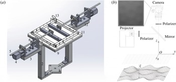
(a) The Faraday waves assembly:
 $1$
, base plate;
 $2$
, vertical column;
 $3$
, horizontal column;
 $4$
, stepper motor;
 $5$
, shaft;
 $6$
, travelling nut connector;
 $7$
, moving walls;
 $8$
, wall connector;
 $9$
, container support rim;
 $10$
, parallel container walls;
 $11$
, container bottom;
 $12$
, U-channel;
 $13$
, injection tube. (b) Optical set-up. The captured digital image corresponds to the rendered pattern at the bottom; the top view of the coloured rendered pattern, i.e. modes
 $(2,6)+(6,2)$
, can be found in figure 6(a).

The experimental set-up should be able not only to produce Faraday waves, but also to change the container dimensions in a time-dependent fashion, as well as to measure the characteristics of the formed patterns. Different components of the designed Faraday assembly presented in figure 3(a) are mounted and function independently on top of the electrodynamic shaker (Labworks ET-139). The liquid is housed in a container with a transparent bottom and four sidewalls, so that inner tank dimensions are
 $150\times 150\times 12.7~\text{mm}^{3}$
without moving walls. As the flatness of the brim plays a crucial role in the formation of Faraday patterns (Douady Reference Douady1990; Bechhoefer et al.
Reference Bechhoefer, Ego, Manneville and Johnson1995), the tank bottom is made of Plexiglas with a flatness precision of 0.05 mm when mounted. Both fixed and moving container walls are machined from Delrin.
The shaker is driven through a linear amplifier (Labworks PA-138). The force rating of the vibration system is 334 N; thus, given the 3.2 kg weight of our assembly and the fluid, the maximum achievable acceleration is about
 $10g$
, well above the range of accelerations
 $0.8$
–
 $1.9~\text{m}~\text{s}^{-2}$
used throughout all the experiments to produce Faraday waves. The acceleration signal is generated by LabView software and then converted to an analogue voltage by a data acquisition device. The actual acceleration of the container is measured by a Brüel and Kjær 4513 accelerometer with accuracy of
 $\pm 1\%$
, interfacing with a 1704-A-001 (Brüel and Kjær) signal conditioner before being sent to the data acquisition device for readout and real-time signal processing with LabView. The latter, using a fitted sinusoidal curve, determines the actual frequency and amplitude of the signal and then compares to the input driving signal showing the frequency difference within
 $0.02\,\%$
and the residual root-mean-square amplitude never exceeding
 $1.0\,\%$
of the driving root-mean-square amplitude thus confirming the absence of stray mechanical harmonics.
Since the shaker is the main source of heat, it is equipped with a cooler pump blowing air through its interior, which in turn helps to maintain the environment temperature unaltered – this, in particular, is important for the constancy of surface tension, otherwise affecting the Faraday waves as per the dispersion relation (1.2). Direct measurement of the temperature with a thermocouple placed at the closest point of the assembly to the shaker, i.e. the aluminum base plate in figure 3(a), showed a temperature variation of
 $22.7{-}22.9\,^{\circ }\text{C}$
during a four-hour-long experiment. All the above three set-up characteristics – the controlled shaker waveform and apparatus temperature as well as flatness of the container brim and bottom – are crucial for the ability to generate reproducible Faraday waves.
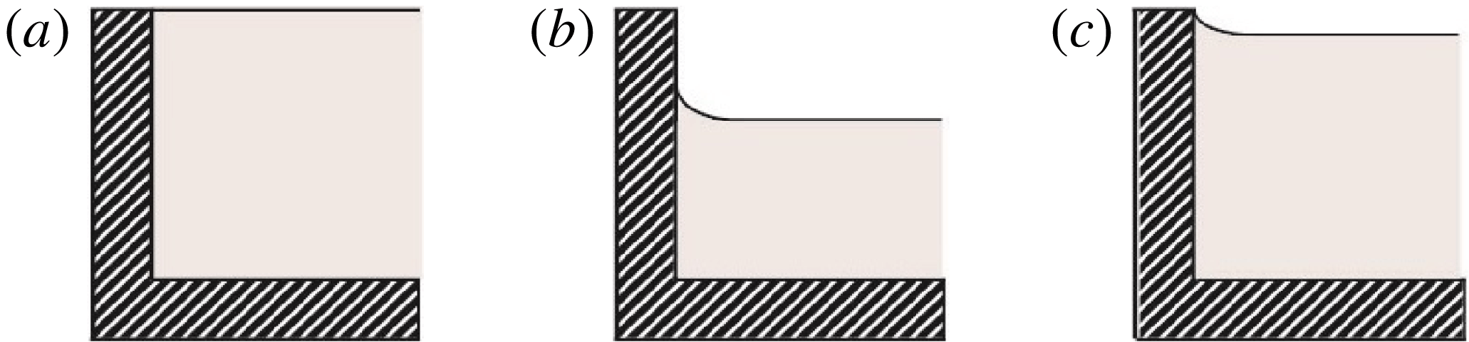
(a) A cross-section of a rectangular container with two moving walls on the left and right; the entire container moves vertically in time. Top (b) and side (c) views of static contact angle near a corner of the domain; the length scale is set by the thickness of the wall being
 $12.7~\text{mm}$
.

The horizontal domain size can be controlled in a time-dependent fashion according to the prescribed laws
 $x_{1}(\unicode[STIX]{x1D70F}_{w})$
and
 $x_{2}(\unicode[STIX]{x1D70F}_{w})$
as per figure 4(a), where
 $\unicode[STIX]{x1D70F}_{w}$
is a long time scale, compared to that of the vertical oscillations. While the locations
 $x_{1}$
and
 $x_{2}$
are independent, in our experiment their implemented motion, controlled by two linear actuators, is symmetric with respect to the centreline of the vessel, i.e.
 $x_{1}=-x_{2}$
. The assembly on each side of the domain (figure 3
a) is comprised of sliding wall, wall connector, shaft, nut connector, leadscrew and stepper motor (NEMA 11), which converts the rotatory motion of the stepper motor into linear motion. The linear actuators enable the walls to travel at speeds between
 $0$
and
 $45~\text{mm}~\text{s}^{-1}$
while keeping their centre of mass over that of the shaker and providing unobstructed optical access from below and above the container. Each stepper motor is driven by a ViX controller (Parker-Hannifin ViX 250IM), which in turn is controlled with Easi-V software. We study the free surface between the movable walls, ignoring the one outside thereby defining our time-dependent spatial domain (figure 4
a).
Considering that the wall motion may generate sloshing waves, great care must be taken to ensure that the Faraday waves are not perturbed; thus, the time scale
 $\unicode[STIX]{x1D70F}_{w}$
of horizontal motion should be necessarily longer than that of the vertical vibration
 $t\ll \unicode[STIX]{x1D70F}_{w}$
. In our experiments, the frequency of the vertical motion is two orders of magnitude greater than that of the prescribed horizontal motion
 $f_{w}=\unicode[STIX]{x1D70F}_{w}^{-1}<0.07~\text{Hz}$
. At this frequency
 $f_{w}$
the amplitude
 $C_{w}$
of the wave induced by wall motion (Ursell, Dean & Yu Reference Ursell, Dean and Yu1960) is only
 $C_{w}=0.01A_{w}$
, where
 $A_{w}$
is the amplitude of the wall motion (see further discussion in § 4.7), ensuring that no sloshing interferes with Faraday waves. Also, to keep the fluid layer depth constant, the moving sidewalls do not reach the bottom of the container, i.e. there exists a clearance of about
 $2~\text{mm}$
allowing unobstructed flow underneath the walls and not affecting Faraday waves (see appendix A).
A few further comments need to be made about water as a working fluid since some practical limitations naturally arise. Namely, when water is exposed to air, it becomes prone to contamination leading to surface tension gradients over the free surface, which in turn complicates the interpretation of the experiments as discussed by Bechhoefer et al. (Reference Bechhoefer, Ego, Manneville and Johnson1995). While we added titanium dioxide (
 $\text{TiO}_{2}$
) to water for visualization purposes (§ 2.2), this chemical neither introduces any surface film effects nor modifies the shear viscosity and surface tension (Przadka et al.
Reference Przadka, Cabane, Pagneux, Maurel and Petitjeans2011); the latter was maintained at a value of
 $71\pm 1~\text{mN}~\text{m}^{-1}$
throughout the experiment with the temperature of the room held constant at
 $23\pm 0.5\,^{\circ }\text{C}$
. As a result, based on Young’s equation, the contact angle is not modified either, which in the static case with and without
 $\text{TiO}_{2}$
was measured as
 $57.5^{\circ }$
and
 $59.5^{\circ }$
, respectively. The use of the same material for manufacturing both fixed and moving container walls guaranteed a uniform contact angle over the entire perimeter. Given the partial wetting, no noticeable capillary rise near the container corners was observed in the static case as verified directly by projecting a fine grating pattern (figure 4
b,c); in the dynamic case, similarly, no significant distortion of the contact line takes place.
Also, when water is used it can be expected that the system would be sensitive to possible evaporation and thus water layer depth changes (Douady Reference Douady1990). Indeed, through the preliminary experiments, we observed that Faraday waves – especially in the pattern competition regime – are sensitive to the depth of water as per the dispersion relation (1.2). Thus, the water level was kept constant at
 $h=12\pm 0.1~\text{mm}$
by utilizing a syringe pump (PHD ULTRA Harvard apparatus) to inject water outside the moving walls (figure 3
a) at the same rate as the evaporation rate determined for the given experimental conditions in the laboratory, i.e.
 $42~\unicode[STIX]{x03BC}\text{l}~\text{min}^{-1}$
.
2.2 Visualization and measurement technique
To quantitatively study Faraday waves, characterization of their global spatial structure and time evolution
 $z=\unicode[STIX]{x1D701}(t,x,y)$
is needed (figure 3
b), with appropriate spatial and temporal resolutions as per the following requirements. First, the technique should be global, i.e. able to measure the interface deformation over the interrogation area of at least
 $150\times 150~\text{mm}^{2}$
. Second, the minimum required accuracy in the vertical direction is
 $0.05~\text{mm}$
, as limited by the measured meniscus wave amplitude at the centre of the tank in the range 0.05–0.2 mm given that the meniscus can move along the sidewall up to
 $0.7~\text{mm}$
(see appendix B). This enables detection of the flat surface as precisely as possible while studying the phase-slip phenomena and thresholds to instability. Third, although throughout the experiment generating waves with large amplitudes is avoided so as to minimize the nonlinear effects and splashing (over the container edge), still the visualization technique should be able to measure waves of relatively large-amplitude
 $\simeq 3~\text{mm}$
observed under certain conditions. Fourth, the temporal resolution should be reasonably fine, i.e. the sampling frequency must be at least
 $5$
to
 $10$
times the driving frequency to be able to study the dynamical behaviour of the system. The last, but not the least, requirement is for the technique to be non-invasive in order to avoid perturbing Faraday waves.
Various visualization and surface measurement techniques have been introduced in the literature to study Faraday waves and yet most of them do not satisfy all the requirements above. For instance, Xia et al. (Reference Xia, Maimbourg, Punzmann and Shats2012) used diffusing light photography (Wright, Budakian & Putterman Reference Wright, Budakian and Putterman1996), in which a diffusive agent – either suspended imaging particles or a small amount (
 ${<}2\,\%$
in volume) of milk – is added to water such that the intensity of light transmitted is inversely proportional to the local depth allowing the surface elevation to be computed from the 2-D intensity distribution. Such a technique works when the distance over which a light ray scatters through a large angle is larger than the surface deflection, but smaller than the liquid layer depth. Also, the highly accurate amplitude measurement method with a resolution of
 $10^{-2}~\text{mm}$
introduced by Douady (Reference Douady1990), which is based on the image obtained from reflection of a thin laser beam at a specific point on the free surface, is local and useful for small wave amplitudes since the maximum measurable slope at the specific point on the free surface is limited by
 $1/\tan (\frac{1}{2}\unicode[STIX]{x1D717})$
, where
 $\unicode[STIX]{x1D717}$
is the angle between the incident laser beam and the vertical axis perpendicular to the surface. Thus, Douady (Reference Douady1990) had to use a separate technique (bicolour stroboscopy) to visualize the entire surface. More recently, a free-surface synthetic schlieren method based on the analysis of the refracted image of a random dot pattern was offered (Moisy, Rabaud & Salsac Reference Moisy, Rabaud and Salsac2009), but among its disadvantages are extreme sensitivity to slight vibrations and application to weak surface deformations only.
Hence, given our considerations and requirements listed above, we resorted to Fourier transform profilometry – a single-shot optical measurement of surface deformation – which has been widely used to visualize and measure water surface waves (Cobelli et al.
Reference Cobelli, Maurel, Pagneux and Petitjeans2009, Reference Cobelli, Pagneux, Maurel and Petitjeans2011; Maurel et al.
Reference Maurel, Cobelli, Pagneux and Petitjeans2009; Przadka et al.
Reference Przadka, Cabane, Pagneux, Maurel and Petitjeans2011). Such a method is based on an optical system composed of a video projector displaying a grating pattern on the surface and a camera recording the reflection of this pattern from the free surface. The distorted grating pattern due to deformation of the liquid surface is then recorded and compared to the reference image (undistorted grating pattern on the flat surface) so as to produce a phase-shift map – the difference between phases of light intensity at each pixel in the two images – from which the height of the deformed surface is reconstructed through an equation relating the phase difference to the object’s height. The greatest challenge experienced while applying this method to water surface is glare, which previously was partially treated by enhancing the water light diffusivity with the addition of
 $\text{TiO}_{2}$
(Cobelli et al.
Reference Cobelli, Maurel, Pagneux and Petitjeans2009; Przadka et al.
Reference Przadka, Cabane, Pagneux, Maurel and Petitjeans2011); however, a considerable amount of glare still remains.
In an effort to improve the accuracy and applicability of the method we came up with a common-optical-axis geometry implementation of Fourier transform profilometry along with an appropriate phase–height relation. As per figure 3(b), a digital video projector (ViewSonic PJD7820HD) with a resolution of
 $1920\times 1080~\text{pixel}^{2}$
produces the sinusoidal fringe pattern on the water surface with interrogation area up to
 $300\times 170~\text{mm}^{2}$
. A DSLR camera (Nikon D5200) with a resolution of
 $6000\times 4000~\text{pixel}^{2}$
provides a record of the phenomena. The images are captured in raw (Nikon electronic) format to prevent unwanted post-processing through the built-in algorithm in the camera, which would reduce the size and quality of the image, because we need to extract the actual, not manipulated, intensities. Then they are developed into raw tagged image file format prior to entering the signal processing algorithm. To make the common-optical-axis geometry possible, i.e. bringing the camera and projector optical axes together, a semi-transparent mirror (standard 50/50 beam splitter) positioned precisely at
 $45^{\circ }$
, with respect to the projector and/or camera axis, was employed. Furthermore, we introduced a proper filtering of light by implementing two linear polarizers – in front of the camera and projector (figure 3
b) – to remove the reflections remaining after the addition of
 $\text{TiO}_{2}$
. This technique was calibrated and proved to be capable of detecting and reconstructing the surface deformation for the interrogation area of
 $300\times 170~\text{mm}^{2}$
with a vertical resolution of
 $0.05~\text{mm}$
and horizontal resolution of
 $0.08~\text{mm}$
, therefore providing an order-of-magnitude improvement in the accuracy compared to the literature (Cobelli et al.
Reference Cobelli, Maurel, Pagneux and Petitjeans2009; Przadka et al.
Reference Przadka, Cabane, Pagneux, Maurel and Petitjeans2011). To achieve a sampling frequency high enough for reconstructing the slow amplitude in the phase-slip study (§ 4.1), we also utilized a faster camera (Blackmagic Pro), with a frame rate of 50 frames per second providing us with an imaging frequency about eight times greater than that of the Faraday wave, and a resolution of
 $4096\times 2304~\text{pixel}^{2}$
. Finally, the flow field resulting from vertical vibrations and sidewall motion is obtained using a particle image velocimetry (PIV) system (TSI, Inc.) based on a dual-pulse Nd:YAG laser (Evergreen 200 mJ) generating a laser light sheet that illuminates tracer particles in the vibrating liquid.
3 Results: Faraday waves on time-fixed domain
The experiments reported in this section serve to (i) characterize the set-up in order to demonstrate its capability in accurately capturing all the dynamical features of interest and (ii) develop a benchmark study of pattern behaviour to provide both the context and comparison with Faraday waves on time-dependent domains in § 4. In particular, before embarking on experiments in time-dependent domains, we need to identify a proper range of frequencies with which to work. Due to the high sensitivity of the Faraday wave system, extreme caution must be taken in selecting proper contact line conditions, especially if one tries to enhance understanding of dynamical phenomena observed experimentally by making comparisons with the available stability theory on time-dependent domains (Knobloch & Krechetnikov Reference Knobloch and Krechetnikov2014, Reference Knobloch and Krechetnikov2015; Krechetnikov & Knobloch Reference Krechetnikov and Knobloch2017). This effort led us to the regime of Faraday waves, which has not been extensively studied despite intimate connection to the classical theory of Benjamin & Ursell (Reference Benjamin and Ursell1954).
3.1 Boundary conditions
Experimental contact line conditions: (a) pinned, (b) non-pinned and (c) semi-pinned.

Early experimental works sought to disentangle the role of boundary conditions from the physics in the bulk of the fluid as they were considered to be a hindrance in observation of Faraday waves (Douady Reference Douady1990; Bechhoefer et al.
Reference Bechhoefer, Ego, Manneville and Johnson1995). According to Douady (Reference Douady1990) two types of boundary conditions for the free surface can be implemented based on the design of our set-up. The first one is the pinned boundary (e.g. brimful) where the vessel is filled to the fullest
 $\unicode[STIX]{x1D701}=0$
, thus preventing the emission of meniscus waves as the boundaries are pinned and the fully flat surface acts as the actual initial condition before vertical vibrations start (Douady Reference Douady1990) (figure 5
a). The advantage of a pinned condition is that the patterns are not perturbed by the menisci and could be described approximately as the product of two sine waves
 $\sin (m\unicode[STIX]{x03C0}x/L_{x})\sin (n\unicode[STIX]{x03C0}y/L_{y})$
, cf. with Benjamin & Scott (Reference Benjamin and Scott1979) and Douady (Reference Douady1990). Implementing such boundaries in practice is very delicate as precise alignment of the walls and brim is required. Minor mechanical imperfections lead to the formation of meniscus waves (Bechhoefer et al.
Reference Bechhoefer, Ego, Manneville and Johnson1995).
The second possible boundary condition is the non-pinned one, where the vessel is not filled completely (figure 5
b). For this boundary condition the theoretical treatment in the case of an inviscid fluid is rather straightforward leading to patterns as products of two cosines (1.3) (Benjamin & Ursell Reference Benjamin and Ursell1954; Douady Reference Douady1990). A considerable disadvantage of this condition is that, as the contact lines are free to move, the imminent meniscus waves are emitted from the walls and perturb the excited patterns and potentially could mask the true threshold of each mode appearance. However, if the capillary length
 $l_{c}=(\unicode[STIX]{x1D70E}/\unicode[STIX]{x1D70C}g)^{1/2}$
is negligible compared to the pattern wavelength, the effect of menisci is minimized and therefore the theory can be used as a reference point.
Using pinned boundaries is preferred since minimizing contact line mobility and meniscus waves effects is desirable. Our set-up, with the pinned boundary condition – vessel filled to the edge of the walls – was able to produce sine patterns over the range of frequencies 7–100 Hz of interest to us without any observable menisci. However, our main objective of conducting experiments on time-dependent domains prevented us from using such boundaries; on a time-fixed domain, when the vessel is filled fully and vibrated vertically by starting from a flat surface with gradual increase in driving amplitude, a transient wave (especially in the low range of frequencies) with an amplitude of several millimetres is formed, though decays quickly upon reaching the stable pattern (Simonelli & Gollub Reference Simonelli and Gollub1989). This transient wave substantially disturbs the fluid domain boundaries by forcing the fluid to flow over the wall edges – the effect which is enhanced by the motion of the walls thus perturbing the whole system. Hence, from an experimental point of view, boundaries cannot be kept fully pinned for all driving conditions. Such considerations led us to a compromise between pinned and non-pinned conditions by setting the waterline 0.7 mm below the wall edge (nearly brimful), thus limiting the meniscus motion, which hereafter will be referred to as a semi-pinned boundary condition (figure 5 c). Depending on driving frequency, it gives either sine- or cosine-type solutions. Below a frequency of 12.1 Hz modes are essentially quantized, the same as for the choice of the boundary conditions in Benjamin & Ursell (Reference Benjamin and Ursell1954), due to the boundedness of the domain, which enables us to study the corresponding discernible stability curves (§ 3.2).
3.2 Road map
In spatially unbounded (in the
 $xy$
plane) systems, there is a continuous spectrum of modes available, while mode quantization is the signature of a finite-size domain (Bechhoefer et al.
Reference Bechhoefer, Ego, Manneville and Johnson1995). Detailed study of pattern formation on a time-dependent domain requires the mode to be far removed from adjacent modes. Since the infinite-domain regime is approximately accessible on any finite domain size if the driving frequency is high enough, we resorted to a lower range of frequencies. Also, pinned boundaries enhance the mode separation markedly (Douady & Fauve Reference Douady and Fauve1988; Douady Reference Douady1990; Bechhoefer et al.
Reference Bechhoefer, Ego, Manneville and Johnson1995) in the sense that the overlap between the stability curves/tongue regions is reduced thus making the modes more distinct; employing semi-pinned boundaries in our set-up contributes to mode separation as well.
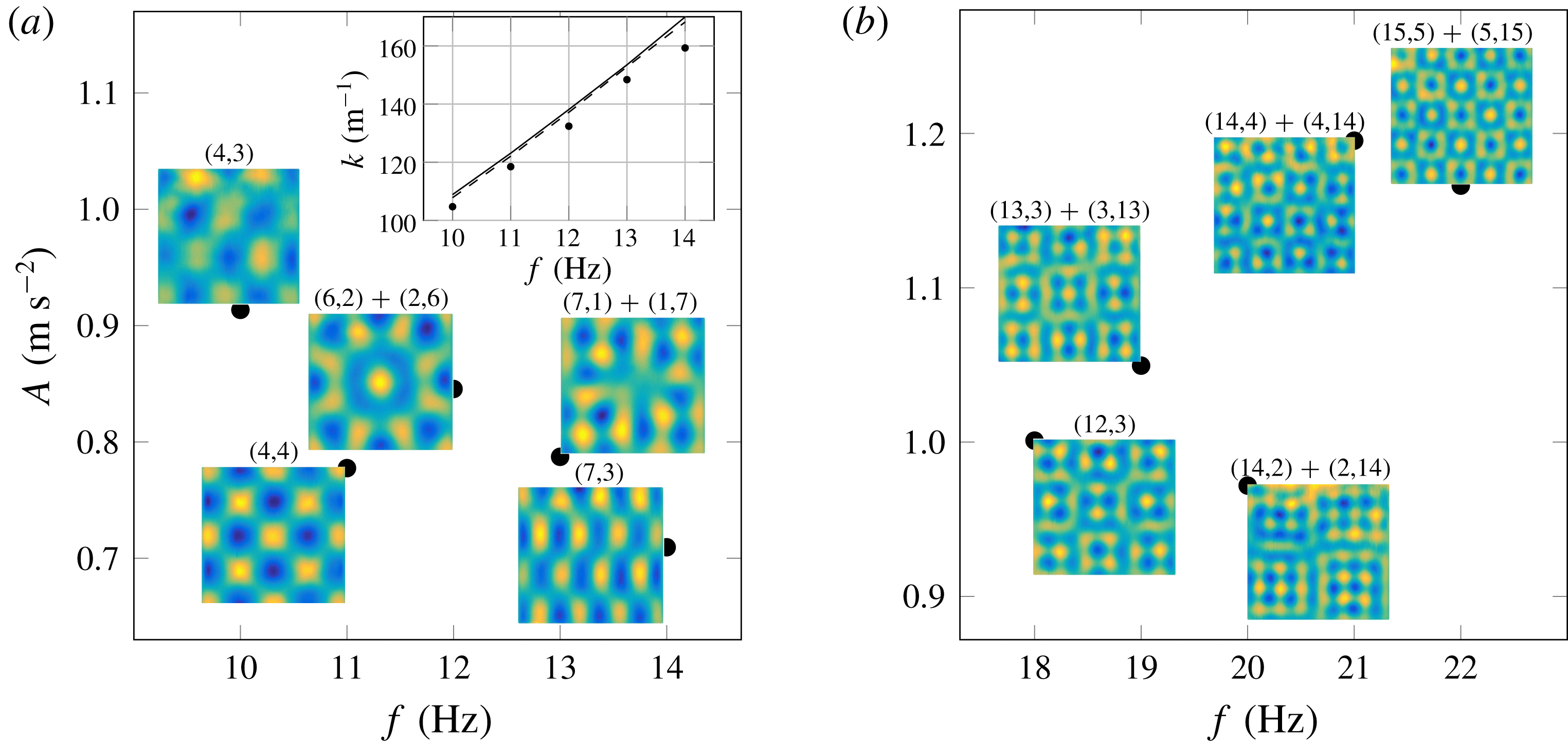
Road map on the square domain: for the studied range of frequencies
 $10$
–
 $22~\text{Hz}$
, depicted are (a) cosine and (b) sine regimes. Each circle represents the measured threshold of vertical acceleration
 $A$
of various modes at a given excitation frequency
 $f$
. The images depict the observed patterns over thresholds. The corresponding mode(s) number is stated on each pattern. Inset in (a) compares the measured wavenumbers (dots) with the critical ones predicted from the viscous theory (solid line) by Kumar & Tuckerman (Reference Kumar and Tuckerman1994) and the inviscid theory (dashed line) by Benjamin & Ursell (Reference Benjamin and Ursell1954).

Figure 6 presents the road map for our experiments, where frequencies ranging from
 $10$
to
 $22~\text{Hz}$
were studied. We found that from
 $10$
to
 $14~\text{Hz}$
cosine-type patterns are formed (figure 6
a), and from
 $18$
to
 $22~\text{Hz}$
sine-type patterns are excited (figure 6
b); the range of intermediate frequencies 14–18 Hz corresponds to the mixed zone, where patterns could not be categorized as either sine or cosine type. Given that the wavenumber
 $k$
depends on
 $(m,n)$
through (1.3), in figure 6 one can see that with an increase in excitation frequency
 $f=2\unicode[STIX]{x03C0}/\unicode[STIX]{x1D714}$
patterns are formed in the order of increasing wavenumber
 $k$
– this is in accordance with the monotonic behaviour of the dispersion relation (1.2) in the cosine regime; a similar statement can be made about the sine regime based on the work of Benjamin & Scott (Reference Benjamin and Scott1979). Obviously, the dissipative effects do not affect the monotonicity of the wavenumber behaviour, which indicates that they are not sufficiently strong in our experiments (Douady Reference Douady1990), see also the discussion in appendix C.
Altogether, observing both types of patterns was made possible by using semi-pinned boundary conditions, which can approximate either pinned or non-pinned boundary conditions depending on the driving frequency. Namely, in the cosine regime (lower mode number with a longer wavelength) the capillary length
 $l_{c}\approx 2.7~\text{mm}$
is negligible compared to a typical wavelength, which is
 $20$
times larger. Also, at these lower frequencies the wave amplitudes are higher, which is easy to see from the real Ginzburg–Landau equation (GLE) describing modulation with amplitude
 $U_{Q}=(\unicode[STIX]{x1D707}-Q^{2})^{1/2}$
and wavenumber
 $Q$
of an excited spatially periodic pattern at the bifurcation parameter
 $\unicode[STIX]{x1D707}$
: clearly, at a fixed
 $\unicode[STIX]{x1D707}$
waves with lower modulation wavenumber
 $Q$
would have a higher amplitude
 $U_{Q}$
. These higher-amplitude waves force the contact line to move hence being closer to non-pinned boundary conditions. On the contrary, in the sine regime the wavelength is varied from
 $7$
to
 $9$
times the capillary length which suggests that capillarity is not negligible. Furthermore, modes that are excited at higher frequencies, i.e. with a larger wavenumber, carry lower wave amplitude thus enabling nearly pinned boundary conditions. It should be noted that all the patterns studied throughout the experiments fall under the category of ‘square patterns’ (Kudrolli & Gollub Reference Kudrolli and Gollub1996) based on their symmetries. Given the rectangular geometry of our container, the low-viscosity fluid used and the low range of frequencies and amplitudes of the single-frequency forcing, the formation of patterns with other symmetries such as hexagonal, stripes and quasi-crystalline is not expected.
The images in figure 6 depict the observed patterns at the corresponding frequencies close to the minimum acceleration required to excite a pattern on the tongue-like threshold curve. However, the non-monotonic behaviour of
 $A(f)$
is the signature of the threshold curve in the low range of frequencies as shown both experimentally and theoretically by Batson, Zoueshtiagh & Narayanan (Reference Batson, Zoueshtiagh and Narayanan2013) based on the work of Kumar & Tuckerman (Reference Kumar and Tuckerman1994). This observation is analogous to similar previous findings in the literature (e.g. Bechhoefer et al.
Reference Bechhoefer, Ego, Manneville and Johnson1995; Batson et al.
Reference Batson, Zoueshtiagh and Narayanan2013) and is mainly due to mode separation, which allows each mode to have its tongue-like stability curve well developed without being early terminated by surrounding stability curves (figure 9). The above-mentioned non-monotonic behaviour is also contributed by the large fluid layer depth, which makes the stability curves less broad because with
 $h$
much larger than the viscous boundary layer thickness
 $\unicode[STIX]{x1D6FF}_{\unicode[STIX]{x1D708}}\sim (\unicode[STIX]{x1D708}/\unicode[STIX]{x1D714}_{0})^{1/2}$
(where
 $\unicode[STIX]{x1D708}$
is the kinematic viscosity) the dissipation at the bottom of the container is not strong enough to broaden the resonance tongue (Bechhoefer et al.
Reference Bechhoefer, Ego, Manneville and Johnson1995).
Dissipation of each mode is proportional to the minimum acceleration required to excite a pattern (Douady Reference Douady1990). For example, in the sine regime, as illustrated in figure 6(b), an increase in the mode number
 $n$
transverse with respect to the direct one
 $m$
, e.g.
 $(m,n)=(14,2)$
to (14,4), leads to an increase in the threshold and correspondingly in dissipation which was also observed in a square cell by Douady & Fauve (Reference Douady and Fauve1988). This fact explains why the formed patterns tend to have a lower transverse mode number: due to their lower dissipation, they can mask the observation of other patterns with greater
 $n$
and thus with larger dissipation. In the sine regime, the system gets closer to the infinite-domain limit due to higher frequencies as mentioned earlier. To keep the system in the quantized regime, the remaining experiments in the paper are restricted to the cosine patterns, which correspond to the classical inviscid theory of Benjamin & Ursell (Reference Benjamin and Ursell1954), see the comparison of the measured and theoretical wavenumbers in the inset of figure 6(a).
3.3 Thresholds
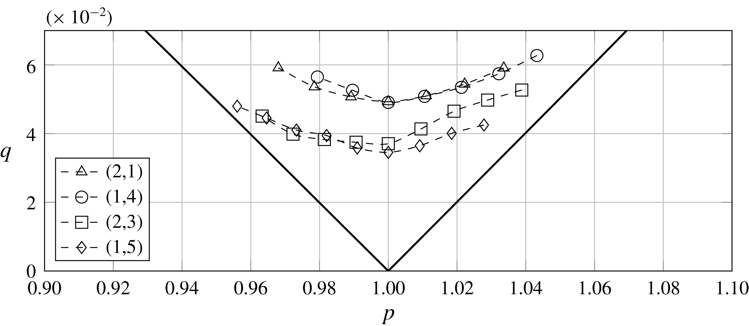
Stability curves for various modes, arranged in increasing order of the total wavenumber (1.3), with the domain aspect ratio
 $R=2.00$
, where
 $p$
and
 $q$
are non-dimensional driving frequency and acceleration, respectively (see equation (3.1)). Dashed lines represent the experimental data, while solid lines represent the stability curve obtained from the linear inviscid theory (Benjamin & Ursell Reference Benjamin and Ursell1954). The threshold curves here and in figure 6 were found starting from a flat surface at a fixed driving frequency and increasing the amplitude until a stable non-flat mode is reached, though Faraday waves are known to possess a hysteretic behaviour in threshold values (Simonelli & Gollub Reference Simonelli and Gollub1989; Craik & Armitage Reference Craik and Armitage1995; Périnet et al.
Reference Périnet, Falcón, Chergui and Juric2016).

Next, the measured stability curves for several modes on the domain of aspect ratio
 $R\equiv L_{y}/L_{x}=2.00$
are presented in figure 7 in the parameter space of dimensionless driving frequency
 $p$
and acceleration
 $q$
:
 $$\begin{eqnarray}p=4\unicode[STIX]{x1D714}_{0}^{2}/\unicode[STIX]{x1D714}^{2}\quad \text{and}\quad q=2kA\tanh (kh)/\unicode[STIX]{x1D714}^{2},\end{eqnarray}$$
where
 $A$
is the dimensional acceleration defined in figure 6. The deviation of the experimental results from the theoretical curve in figure 7 is due to the inviscid fluid approximation and infinitesimal wave amplitude assumed by Benjamin & Ursell (Reference Benjamin and Ursell1954). For each mode, the tongue-like curve (figure 9) is well established and terminated by the excitation of previous/next mode. Minimum of each curve corresponds to the resonance frequency and the minimum dissipation of the mode. Similar to the square domain case, these modes were observed in the order of increasing wavenumber
 $k$
with the driving frequency
 $f$
. This fact suggests that even in this smaller domain size the influence of walls is minimized in our experiment; otherwise, non-monotonic shifts in both wavenumbers and dissipation would be observed (Douady Reference Douady1990). The shifts observed in dissipations – e.g. mode (1,4) appears to have higher dissipation than (1,5) in figure 7 – can be explained similarly to the discussion in § 3.2; the non-monotonic behaviour of dissipation is the signature of the threshold curve at low frequencies (Batson et al.
Reference Batson, Zoueshtiagh and Narayanan2013).
3.4 Symmetric mode interactions
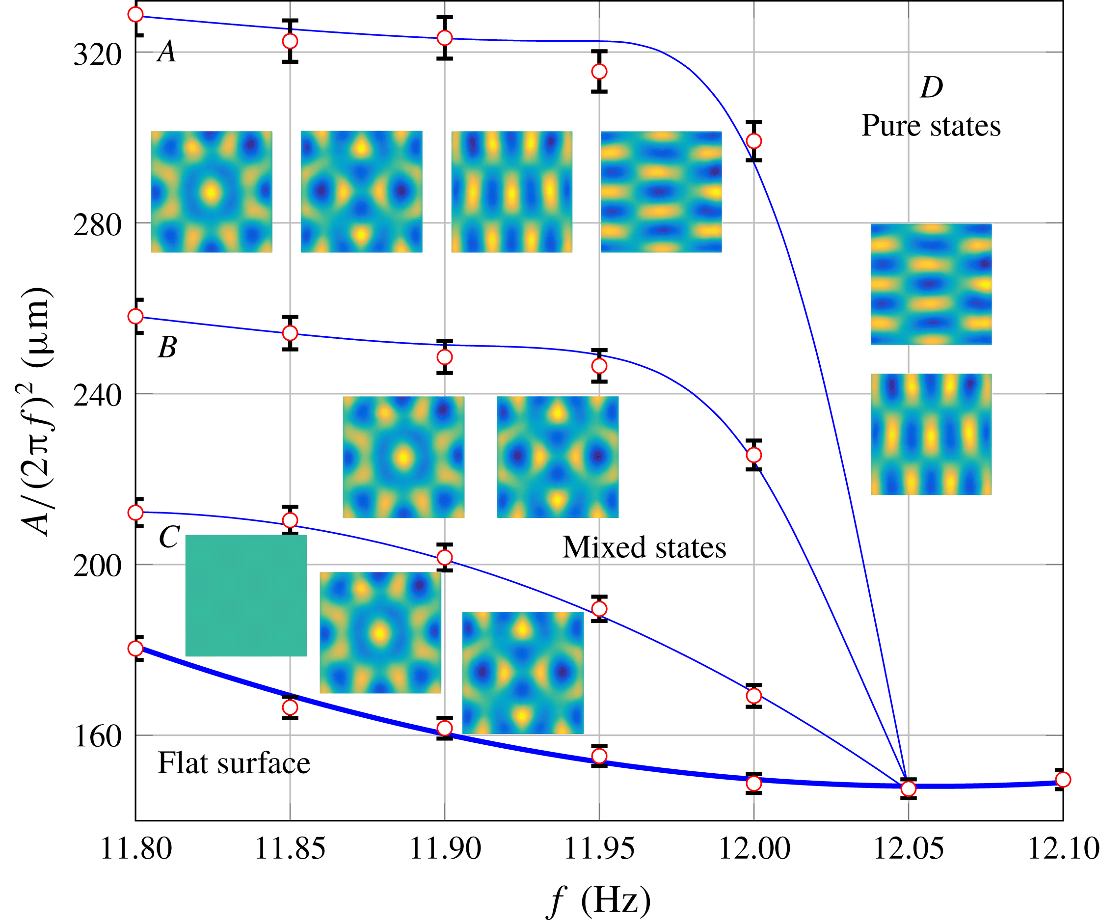
Amplitude–frequency diagram around mode (6,2) and its symmetric one (2,6) on a square domain. Four regions exist above threshold: mixed states
 $B$
and pure states
 $D$
, and two hysteresis ones
 $A$
and
 $C$
. The circles represent the experimental data with the error bars corresponding to the accuracy of the measurements; the solid lines through the data sets are meant just to guide the eye. The images represent the typical patterns observed in the region and each can be formed in the corresponding region depending on the initial driving frequency and amplitude.

Previous works on Faraday waves focused primarily on dynamical behaviours of the system such as bifurcations, mode interactions and pattern competition which lead to chaos under certain conditions. For instance, Simonelli & Gollub (Reference Simonelli and Gollub1989) in their experimental work on the interactions between two symmetric modes
 $(m,n)$
and
 $(n,m)$
naturally excited on a square domain were able to unravel the differences of the phase-space structure between square and slightly non-square containers. As it will be important for our study on time-dependent domains in the vicinity of pattern competition regime (§ 4.3), we provide here a detailed study of the interactions between symmetric modes (2,6) and (6,2), as they are sufficiently away from excitation of adjacent modes (figure 8). The interactions of such modes can reveal up to
 $16$
fixed points, either stable or unstable, in the corresponding phase space (Simonelli & Gollub Reference Simonelli and Gollub1989). The discussion here parallels that from the above reference on the interaction of modes (2,3) and (3,2). Obviously (Simonelli & Gollub Reference Simonelli and Gollub1989), excitation of a pure mode, e.g. (2,6), or interaction between two modes, e.g.
 $(6,2)+(2,6)$
, corresponds to two fixed points, one with positive and the other with negative amplitude.
Referring to figure 8, four distinct regions are observed above the threshold. In region
 $D$
either of the pure states, (6,2) or (2,6), is formed depending on the initial conditions. In region
 $B$
mixed states, where two modes interact either in phase
 $(6,2)+(2,6)$
or out of phase
 $(2,6)-(6,2)$
, are found. Observation of both in-phase and out-of-phase combinations of these two modes is in accordance with the analytical analysis of Feng & Sethna (Reference Feng and Sethna1989), who showed that on a square domain
 $D_{4}$
symmetry can be expected, i.e. if the in-phase interaction
 $(m,n)+(n,m)$
is allowed by the system then all the other combinations – in-phase
 $-(m,n)-(n,m)$
along with out-of-phase
 $(m,n)-(n,m)$
and
 $-(m,n)+(n,m)$
– can be formed as well. However, Simonelli & Gollub (Reference Simonelli and Gollub1989) claimed, based on the symmetry analysis, that when both
 $m$
and
 $n$
are odd or even (as in our case), only one of the in-phase or out-of-phase cases is possible, which is one of the differences between their analysis and that by Feng & Sethna (Reference Feng and Sethna1989). Even experimentally, Simonelli & Gollub (Reference Simonelli and Gollub1989) observed only out-of-phase mixed state for even mode numbers, (0,4) and (4,0). Nevertheless, they pointed out that due to excitation of nearby modes such types of interactions could not be investigated thoroughly, which may have prevented them from detecting the in-phase combination. Later Miles & Henderson (Reference Miles and Henderson1990) proved that symmetry analysis performed by Simonelli & Gollub (Reference Simonelli and Gollub1989) is incomplete leading to differences from that of Feng & Sethna (Reference Feng and Sethna1989). Regardless, as follows from figure 8, in our experiment we were able to observe both in- and out-of-phase mixed states in region
 $B$
, where the mixed states are stable fixed points and the pure modes become saddle points.
Regions
 $A$
and
 $C$
are hysteretic: namely, if one starts from below the threshold curve at a frequency less than
 $12.05~\text{Hz}$
and increases the amplitude, in region
 $C$
a flat surface would be observed, but if the starting point is in region
 $B$
, then by decreasing the amplitude and entering region
 $C$
mixed states would be expected. In region
 $A$
eight stable fixed points are observed (both mixed and pure states), while in region
 $C$
only five stable fixed points – the pure modes and the flat surface – exist. It should be noted that images in figure 8 depict the typical patterns observed, but due to the hysteretic behaviour each can be formed in the corresponding region depending on the initially chosen driving frequency and amplitude.
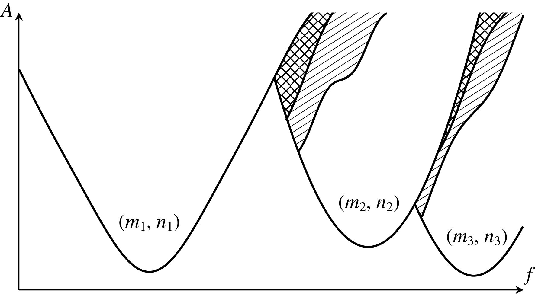
Schematic representation of figure 2 of Ciliberto & Gollub (Reference Ciliberto and Gollub1984) based on experiments on a circular domain with a radius of 6.35 mm. For each mode
 $(m,n)$
solid curve denotes stability boundaries in the driving frequency
 $f$
and acceleration
 $A$
coordinates. Single/double dashed regions represent the periodic/chaotic pattern competition regimes of two adjacent modes.

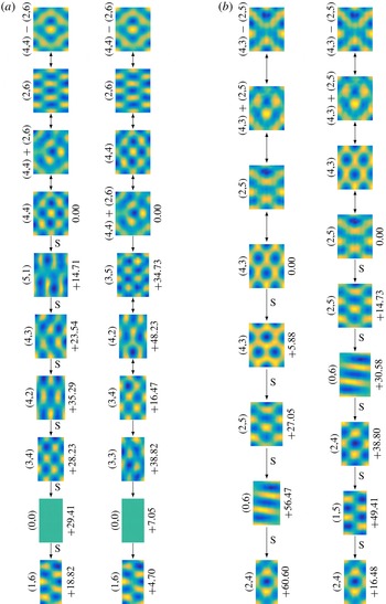
Simultaneous excitation of two adjacent modes at the same values of physical parameters takes place in the overlap region of the two stability curves known as a pattern competition regime (dashed areas in figure 9), which is very common in Faraday wave phenomena as shown by Ciliberto & Gollub (Reference Ciliberto and Gollub1985b ), whose phenomenological model is able to reproduce it. In this regime slow amplitudes of two different patterns are non-zero, non-equal and oscillate with different phases at a frequency smaller than the driving one by more than two orders of magnitude (Ciliberto & Gollub Reference Ciliberto and Gollub1984, Reference Ciliberto and Gollub1985a ). An example of patterns observed in such a region in our experiments can be seen in figure 12(c) with the cycling of patterns illustrated by up–down arrows.
When performing experiments on a square domain we did not detect any time-dependent patterns as expected due to symmetry (Simonelli & Gollub Reference Simonelli and Gollub1989). However, despite the fact that Simonelli & Gollub (Reference Simonelli and Gollub1989) could not find any time-independent superposition (stable fixed point) of the two specific symmetric modes (3,2) and (2,3) in a nearly square cell, we found one specific case where the interaction between modes (2,6) and (4,4) was time-independent (stable fixed point) for the domain aspect ratio
 $R=1.25$
. Our observation is in agreement with the theory of Feng & Sethna (Reference Feng and Sethna1989) which predicts that time-independent mixed states can be expected in a non-square domain as well depending on the detuning frequency (the frequency difference from the resonance frequency of one of the modes) and the domain aspect ratio. Furthermore, for the specific case of interaction between modes (3,2) and (2,3), studied by Simonelli & Gollub (Reference Simonelli and Gollub1989), the resonant frequencies between these modes differed by 1.5 % whereas for modes (4,4) and (2,6) in our experiment the difference is only 1 % which brings the stability curves closer. This makes the pattern competition region sizable enough (e.g. compared to the Simonelli & Gollub (Reference Simonelli and Gollub1989) study) that finite-amplitude perturbations always present in real experiments are not sufficient to destabilize the superposition of modes (2,6) and (4,4).
The threshold curves in figure 8 were measured using a manual and simpler method than the automated scanning protocol based on the successive approximation applied by Simonelli & Gollub (Reference Simonelli and Gollub1988, Reference Simonelli and Gollub1989). At a fixed driving frequency a low driving amplitude, at which a non-flat surface first forms, is found by increasing it from below – this is assigned as an upper bound for the threshold. Then, the amplitude is decreased to arrive at the flat surface which yields yet another bound for the threshold termed as a lower one since it proves to be below the previously found upper bound. Finally, the amplitudes between upper and lower bounds are scanned with successively reduced positive and negative amplitude increments to identify possible hysteresis regions and to measure the instability boundaries.
3.5 Summary
Our search for a suitable Faraday waves regime led us to (i) moderate-aspect-ratio waves, i.e. with the wavelengths
 $\unicode[STIX]{x1D706}$
not significantly smaller than the domain size as opposed to the widely studied large-aspect-ratio regime (Douady & Fauve Reference Douady and Fauve1988; Douady Reference Douady1990; Edwards & Fauve Reference Edwards and Fauve1994; Kudrolli & Gollub Reference Kudrolli and Gollub1996; Binks & van de Water Reference Binks and van de Water1997) thus enabling pronounced square mode separation; (ii) but still with considerably longer wavelengths compared to the capillary length
 $l_{c}$
in order to minimize the effect of capillarity on the boundary conditions, since wetting details upset the Benjamin & Ursell (Reference Benjamin and Ursell1954) theory leading to non-analytical modes (Benjamin & Scott Reference Benjamin and Scott1979; Douady & Fauve Reference Douady and Fauve1988; Douady Reference Douady1990); and (iii) the use of low-viscosity fluids with the goal to match to the classical theory (Benjamin & Ursell Reference Benjamin and Ursell1954) amenable to transparent analytical treatment. The accuracy of the inviscid dispersion relation (1.2) applied to our case is demonstrated in the inset of figure 6(a), which again indicates negligible role of menisci in the sense of deviation from the inviscid contact line conditions assumed by Benjamin & Ursell (Reference Benjamin and Ursell1954). As demonstrated in appendix C, for our low driving frequency experiments viscous theory (Kumar Reference Kumar1996) would not modify the quantitative behaviour of the stability curve noticeably compared to that of the inviscid one (Benjamin & Ursell Reference Benjamin and Ursell1954; Batson et al.
Reference Batson, Zoueshtiagh and Narayanan2013); thereby, the linear inviscid theory can be used as the reference for our framework. Working in this classical regime, stripped of any complexities associated with appearance of hexagonal, quasi-periodic, quasi-crystal and chaotic modes, is necessary to make the domain evolution effects distinguishable. Also, while above we used, in particular, a square container to prove the accuracy of the experimental set-up, due to the degeneracy of a square domain (Simonelli & Gollub Reference Simonelli and Gollub1987), which makes the system very sensitive to small symmetry-breaking perturbations thus dramatically affecting the dynamics, we will study the domain evolution effects on rectangular domains only.
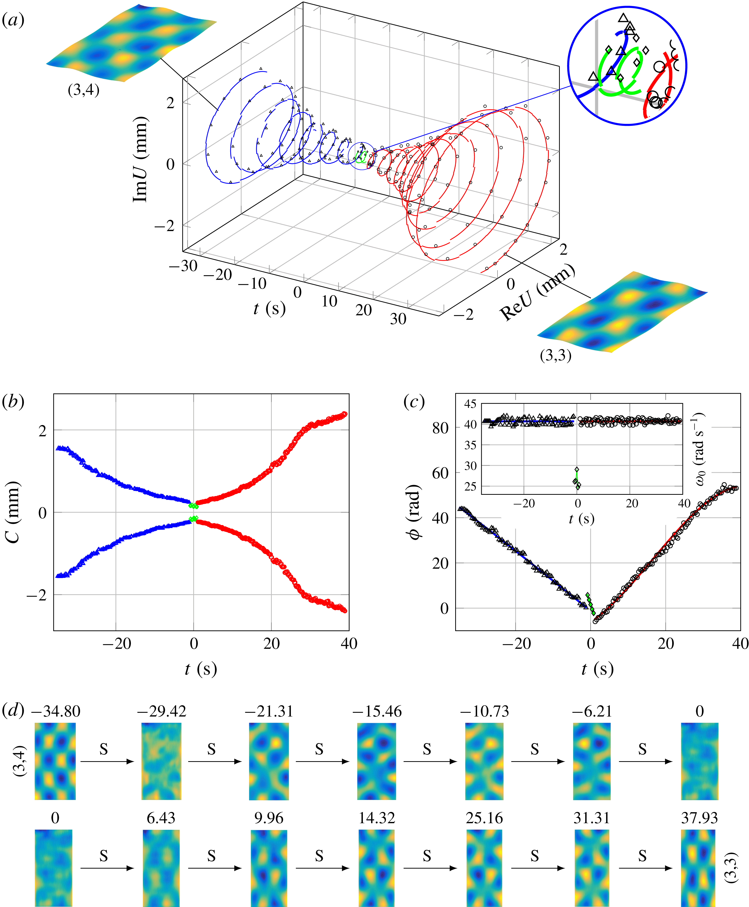
Phase-slip event on the time-dependent domain at driving frequency 12.95
 $\text{Hz}$
, amplitude
 $1.4~\text{m}~\text{s}^{-2}$
and wall speed
 $0.03~\text{mm}~\text{s}^{-1}$
for the mode change from (3,4) to (3,3). Data recovered from the experiment are represented by different symbols: mode (3,4), triangles; mode (3,3), circles; and the phase-slip event during which only meniscus waves are detectable, diamonds. Solid lines are the fitted curves through the data. (a) The complex amplitude
 $U$
, in which the imaginary and real parts are the slow amplitudes of the above modes. (b) The total amplitude envelope
 $C(t)$
. Wave phase
 $\unicode[STIX]{x1D719}$
and its frequency
 $\unicode[STIX]{x1D714}_{0}$
are presented in (c) and the inset, respectively. (d) Representation of pattern evolution: the top row depicts the destruction of mode (3,4) and the bottom row shows formation of mode (3,3). On the top of each mode the corresponding time at which the given pattern is observed is stated. The time origin is defined to be the mid-point of the phase-slip event.

4 Results: Faraday waves on time-dependent domain
Given that previous theoretical efforts have mainly focused on dynamical properties on one-dimensional (1-D) time-dependent domains (Knobloch & Krechetnikov Reference Knobloch and Krechetnikov2014, Reference Knobloch and Krechetnikov2015; Krechetnikov & Knobloch Reference Krechetnikov and Knobloch2017), we now resort to Faraday waves with the aim of understanding the following key effects of domain deformation in two dimensions: domain shrinkage–growth, domain evolution rate, domain oscillation and interaction of domain time dependence with a pattern competition regime.
4.1 Phase-slip phenomena
Interpretation of the subsequent experimental results requires an understanding of the pattern destruction/formation mechanism known as a phase slip which will be considered in detail in this subsection. On a time-fixed domain, given a phase-winding solution for the order parameter
 $U(\unicode[STIX]{x1D70F},\unicode[STIX]{x1D743})=C(\unicode[STIX]{x1D70F},\unicode[STIX]{x1D743})\text{e}^{-\text{i}\unicode[STIX]{x1D719}(\unicode[STIX]{x1D70F},\unicode[STIX]{x1D743})}$
representing a spatially periodic pattern of amplitude
 $C(\unicode[STIX]{x1D70F},\unicode[STIX]{x1D743})$
and phase
 $\unicode[STIX]{x1D719}(\unicode[STIX]{x1D70F},\unicode[STIX]{x1D743})$
dependent on slow time
 $\unicode[STIX]{x1D70F}=\unicode[STIX]{x1D716}^{2}t$
and spatial
 $\unicode[STIX]{x1D743}=\unicode[STIX]{x1D716}\boldsymbol{x}$
variables with
 $\unicode[STIX]{x1D716}\ll 1$
, a cell in a particular
 $x$
-direction can only be created or destroyed via the Eckhaus instability (Eckhaus Reference Eckhaus1965). This happens at the locations where the order parameter
 $U(\unicode[STIX]{x1D70F},\unicode[STIX]{x1D743})$
vanishes,
 $\text{Re}U(\unicode[STIX]{x1D70F},\unicode[STIX]{x1D743})=\text{Im}U(\unicode[STIX]{x1D70F},\unicode[STIX]{x1D743})=0$
, so that the phase-winding spiral intersects the
 $x$
-axis (Langer & Ambegaokar Reference Langer and Ambegaokar1967) and hence the local spatial phase
 $\unicode[STIX]{x1D719}(\unicode[STIX]{x1D70F},\unicode[STIX]{x1D743})$
is undefined, the event usually named as a phase slip. A phase slip inserts a new wavelength (cell) into the pattern after relaxation resulting in a new pattern with a shorter wavelength. When this wavelength falls in the Eckhaus-stable region, no further phase slips will be triggered.
Effects of the domain time dependence (Knobloch & Krechetnikov Reference Knobloch and Krechetnikov2014) can enter in the above picture in the following two ways. First, a gradual growth of the domain leads to repeated phase slips as the pattern tries to keep its wavelength in the preferred, Eckhaus-stable, range. Second, since the phase slips occur on a fast time scale (the Eckhaus instability is subcritical), the number of phase slips that occur before stability is restored depends on the delay in triggering the instability. Local analysis reveals that compared to the time-independent domain case, time evolution of the spatial extent of the system delays the occurrence of a phase slip when the domain is growing (Knobloch & Krechetnikov Reference Knobloch and Krechetnikov2014; Krechetnikov & Knobloch Reference Krechetnikov and Knobloch2017) and accelerates when the domain is shrinking. Moreover, in the presence of dilution and convection, a modified near-critical amplitude equation of the GLE type for the order parameter
 $U$
, derived by Krechetnikov & Knobloch (Reference Krechetnikov and Knobloch2017), possesses new solutions compared to the standard GLE, including spatially periodic solutions with a time-dependent wavenumber and spatially non-periodic (spatially localized) steady states. Also, the effect of the domain size oscillations is always destabilizing in the sense that the band of stable wavenumbers is always reduced, an effect that enhances with decreasing domain oscillation frequency.
A phase-slip event on a time-dependent domain is analysed in figure 10 in the vicinity of the mode change from (3,4) to (3,3) as an example. With the surface deformation (1.3), the complex slow amplitude function is defined as
 $$\begin{eqnarray}U(\unicode[STIX]{x1D70F})=C(\unicode[STIX]{x1D70F})\text{e}^{-\text{i}\unicode[STIX]{x1D719}(\unicode[STIX]{x1D70F})},\end{eqnarray}$$
where the real amplitude
 $C$
and phase
 $\unicode[STIX]{x1D719}$
depend on the slow time scale
 $\unicode[STIX]{x1D70F}$
(Feng & Sethna Reference Feng and Sethna1989; Simonelli & Gollub Reference Simonelli and Gollub1989). On a time-dependent domain when the time scale of the wall motion
 $\unicode[STIX]{x1D70F}_{w}$
is comparable with
 $\unicode[STIX]{x1D70F}$
, one can expect that phase slip would take place and the present pattern changes to another. To investigate such an event in detail, the real and imaginary parts of the complex slow amplitude
 $U(\unicode[STIX]{x1D70F})$
from the measurements need to be reconstructed as follows. First the total amplitude
 $a=C(\unicode[STIX]{x1D70F})\cos [\unicode[STIX]{x1D714}_{0}t+\unicode[STIX]{x1D719}(\unicode[STIX]{x1D70F})]$
and the time stamps are extracted from each movie frame; then the amplitude envelope
 $C$
, wave frequency
 $\unicode[STIX]{x1D714}_{0}$
and phase
 $\unicode[STIX]{x1D719}$
are recovered (for each two fast cycles separately). Finally,
 $\text{Re}U$
and
 $\text{Im}U$
are determined based on (4.1).
Our visualization technique with a high sampling rate (§ 2.2) allowed us to recover the expected spiral behaviour of
 $U$
(Langer & Ambegaokar Reference Langer and Ambegaokar1967; Knobloch & Krechetnikov Reference Knobloch and Krechetnikov2015; Krechetnikov & Knobloch Reference Krechetnikov and Knobloch2017) during the mode change as presented in figure 10(a), where different symbols – triangles, circles and diamonds – depict modes (3,4), (3,3), and the meniscus waves close to the phase slip, respectively. In addition, solid lines represent curves fitted through the data. The mode change process on the shrinkage path (figure 10
a) starts from the stage at which mode (3,4) is established with constant amplitude and frequency (the measured Faraday wave frequency is
 $40.67~\text{rad}~\text{s}^{-1}$
, which is very close to
 $40.68~\text{rad}~\text{s}^{-1}$
expected from (1.2); see inset of figure 10
c). From the inset of figure 10(c) we can also see that during mode changing the wave frequency remains reasonably close to half of the driving frequency.
During the phase-slip event, in agreement with the above theoretical considerations, both real and imaginary parts of the slow amplitude vanish (figure 10
a,b). It should be noted that the discernible small-amplitude
 ${\approx}0.2~\text{mm}$
meniscus waves at the phase-slip event, depicted by diamonds, are comparable to the accuracy of our measurement technique in this specific experiment (due to the lower resolution of the fast camera used). Because of that and the nature of these waves, we do not comment on the frequency/phase associated with these data points.
The phases recovered for modes (3,4) and (3,3) are presented in figure 10(c). Curve fitting the data to polynomial functions we find
 $\unicode[STIX]{x1D719}_{(3,4)}=2.89\times 10^{-5}t^{3}+5.08\times 10^{-4}t^{2}-1.32t-1.2072$
and
 $\unicode[STIX]{x1D719}_{(3,3)}=-0.0011t^{3}+0.0532t^{2}+1.0859t-6.1170$
, in which all the coefficients in front of
 $t^{n}$
have the units of
 $(\text{rad}~\text{s}^{-n})$
. With the introduction of the non-dimensional fast time
 $\overline{t}=\unicode[STIX]{x1D714}_{0}t$
, the phases read
 $\unicode[STIX]{x1D719}_{(3,4)}=4.3\times 10^{-10}\overline{t}^{3}+3.07\times 10^{-7}\overline{t}^{2}-0.0326\overline{t}-1.2072$
and
 $\unicode[STIX]{x1D719}_{(3,3)}=-1.59\times 10^{-8}\overline{t}^{3}+3.21\times 10^{-5}\overline{t}^{2}+0.0267\overline{t}-6.1170$
, from where the dominant terms are
 $\unicode[STIX]{x1D719}_{(3,4)}\approx -0.0326\overline{t}-1.2072$
and
 $\unicode[STIX]{x1D719}_{(3,3)}\approx 0.0267\overline{t}-6.1170$
. Thus the non-dimensional slow time scale for the phase functions
 $\overline{\unicode[STIX]{x1D70F}}=\unicode[STIX]{x1D716}^{2}\overline{t}$
as defined in the GLE derivation (Cross & Hohenberg Reference Cross and Hohenberg1993) yields
 $\unicode[STIX]{x1D716}_{(3,4)}=0.18$
and
 $\unicode[STIX]{x1D716}_{(3,3)}=0.16$
. These values demonstrate a faster dependence on time compared to a stable Faraday pattern on a fixed domain (for example, see Ciliberto & Gollub (Reference Ciliberto and Gollub1985a
), where
 $\unicode[STIX]{x1D719}(\overline{\unicode[STIX]{x1D70F}})=0.008\overline{\unicode[STIX]{x1D70F}}$
or equivalently
 $\unicode[STIX]{x1D716}=0.09$
) implying that the pattern formation time scale
 $\unicode[STIX]{x1D70F}$
on a time-dependent domain is enslaved by that of wall motion
 $\unicode[STIX]{x1D70F}_{w}$
. Furthermore, the data in figure 10(c) indicate a jump in phase of about
 $1.95\unicode[STIX]{x03C0}$
confirming the theoretical understanding that the phase is undefined at the phase slip and experiences a
 $2\unicode[STIX]{x03C0}$
jump.
At the fundamental level, the observed phase slips correspond to phase transitions of the second kind, which are characterized by scale invariance at the critical point, i.e. possess conformal symmetry – invariance under local scale transformations, while preserving angles between any two vectors (Francesco, Mathieu & Sénéchal Reference Francesco, Mathieu and Sénéchal1997). In other words, the phenomena at the critical point become renormalizable. Naturally, in our context the only free surface that satisfies this scale-invariance requirement is flat thus explaining the peculiarity of the observed phase-slip phenomena when one pattern transforms into another.
4.2 Transverse instability
Examples of (a) a direct mode change
 $(2,5)\rightarrow (1,5)$
with the corresponding amplitude change
 $2.12\rightarrow 1.7~\text{mm}$
and (b) a transverse one
 $(3,3)\rightarrow (3,2)$
with the amplitude change
 $1.37\rightarrow 1.6~\text{mm}$
, both observed during domain shrinkage (S) in the
 $x$
direction. Scale bars are in mm.

Given the detailed mechanism of the mode change on time-dependent domains we can now focus on pattern deformations during shrinkage and growth paths. As discussed in § 2.1, the set-up design allows us to modulate the domain size in a time-dependent fashion in one direction
 $x$
. In the course of domain shrinkage or growth many mode changes occur; however, in this subsection we specifically focus on the ones that have the form of either
 $(m,n)$
to
 $(m\pm 1,n)$
or
 $(m,n)$
to
 $(m,n\pm 1)$
, henceforth named direct and transverse consecutive mode changes, respectively (see figure 11). Under the experimental conditions of driving frequency
 $12.95~\text{Hz}$
, amplitude
 $1.4~\text{m}~\text{s}^{-2}$
and wall speed
 $0.03~\text{mm}~\text{s}^{-1}$
, on the domain shrinkage path
 $R=1.25\rightarrow 2.50$
a sequence of the transverse mode changes
 $(3,4)\rightarrow (3,3)\rightarrow (3,2)\rightarrow (3,1)$
was found. The direct consecutive mode change
 $(m,n)\rightarrow (m\pm 1,n)$
was observed only in the case of
 $(1,5)\leftrightarrow (2,5)$
at a frequency of
 $11~\text{Hz}$
and amplitude of
 $1.32~\text{m}~\text{s}^{-2}$
.
The first significant observation is that regardless of whether the domain is growing or shrinking in the
 $x$
direction, the system tends to change its mode transversely in the
 $y$
direction
 $(m,n)\rightarrow (m,n\pm 1)$
, whence is referred to as a transverse instability. It appears that transverse instability is intrinsic to 2-D systems. The direct consecutive mode change,
 $(m,n)$
to
 $(m\pm 1,n)$
, was highly rare and the single case
 $(2,5)\rightarrow (1,5)$
that we were able to find only happens above some specific wall speed threshold, which is markedly different between domain shrinkage and growth. Namely, during domain growth, the mode change
 $(1,5)\rightarrow (2,5)$
takes place for a wall speed above
 $0.18~\text{mm}~\text{s}^{-1}$
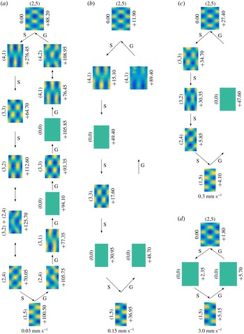
(figure 13
c); the opposite mode change
 $(2,5)\rightarrow (1,5)$
shown in figure 13(c) occurs during domain shrinkage only with a wall speed above
 $2.4~\text{mm}~\text{s}^{-1}$
, an order of magnitude greater. Below these speeds intermittent patterns, either modes (2,4) or (4,1), are formed. The explanation for such a difference between wall speed thresholds is provided in § 4.4.
A basic reason for the observed transverse instability follows from the linear theory. Namely, since subharmonic Faraday waves have their frequency
 $\unicode[STIX]{x1D714}_{0}$
fixed at half of the driving one
 $\unicode[STIX]{x1D714}$
, from the dispersion relation (1.2), where the wavenumber
 $k$
is the modulus
 $k=(k_{x}^{2}+k_{y}^{2})^{1/2}$
of the 2-D wavenumber
 $\boldsymbol{k}=(k_{x},k_{y})$
, it follows that
 $k$
must be fixed as well. With domain evolution in the
 $x$
direction the wavenumber component
 $k_{x}$
gets stretched as allowed by the presence of the domain dilution (Krechetnikov & Knobloch Reference Krechetnikov and Knobloch2017), and thus the wavenumber
 $k_{y}$
in the
 $y$
direction should adjust itself accordingly in order to keep the magnitude
 $k$
constant leading to the transverse instability. Intrinsically, the mechanism for the transverse mode change is due to an Eckhaus instability; while the direct mode wavelength can be stretched/shrunk, the transverse one is pushed in the Eckhaus-unstable region entailing a phase slip and hence a creation/annihilation of a cell (provided that this wavelength is closer to the Eckhaus-unstable region compared to the direct one).
Finally, it must be noted that the transverse instability discussed here differs from the transverse amplitude modulation instability, analysed by Ezerskii et al. (Reference Ezerskii, Rabinovich, Reutov and Starobinets1986) and Milner (Reference Milner1991), which is zigzag as opposed to longitudinal (Eckhaus). Namely, in the case of the 1-D zigzag instability, bending of a roll at an unstable wavelength achieves a shorter (than the original) wavelength in the stable region (Hoyle Reference Hoyle2006), i.e. it is not possible to make up for a shortening of the original wavelength as happens in our transverse instability. In the 2-D situation, as shown by Hoyle (Reference Hoyle1993) on a square domain, the zigzag instability is a direct equivalent of its 1-D counterpart since at the leading order the zigzag instability of each set of rolls is decoupled from the other one; hence the same wavelength shortening takes place. In our case, however, the mechanism driving the transverse instability originates from maintaining the 2-D pattern wavenumber as dictated by the dispersion relation, though some wavenumber variation is allowed due to quantization on a finite domain (Tuckerman & Barkley Reference Tuckerman and Barkley1990).
4.3 Irreversibility
The difference in the behaviour between domain growth and shrinkage observed in the previous subsection brings about the broader topic of reversibility of the sequence of patterns formed on the shrinkage versus growth paths. Reversibility is understood here in the sense that patterns observed on the shrinkage and growth paths ought to be the same. For the experimental conditions of driving frequency
 $11~\text{Hz}$
, acceleration
 $1.32~\text{m}~\text{s}^{-2}$
and wall speed
 $0.15~\text{mm}~\text{s}^{-1}$
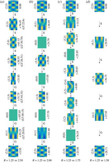
, we studied domain shrinkage and growth between four distinct domain ratios; the observed patterns on each path shown in figure 12 reveal that, in general, domain shrinkage–growth is not reversible. For example, in the case
 $R=1.25\;\Longleftrightarrow \;2.50$
(figure 12
a), the initial and final patterns are the same, but the shrinkage
 $(2,5)\rightarrow (3,3)\rightarrow (2,4)\rightarrow (1,5)\rightarrow (2,2)$
and growth
 $(2,2)\rightarrow (1,5)\rightarrow (0,0)\rightarrow (4,1)\rightarrow (2,5)$
paths are not the reverse of each other. Such an irreversibility can also be seen in figure 12(b,c), while in figure 12(d) the paths are reversible. The latter exception stems from a very short (in space) path preventing the wavenumber from being shifted far away from that on the time-fixed domain, so that we cannot expect many mode changes, especially in the low-frequency regime in which mode separation is prominent.
Pattern observed on domain shrinkage (S) and growth (G) paths, for four domain aspect ratios. Up–down arrows indicate pattern competition regime. For each image of the pattern scaled proportionally to its instantaneous aspect ratio, the mode number is stated on its left and the number on the right denotes the formation time difference
 $\unicode[STIX]{x0394}t$
between the given mode and the previous mode on the path. In (a) we also show the lifetime (
 $LT$
) of each pattern. The experimental fixed parameters are frequency
 $11.00~\text{Hz}$
, acceleration
 $1.32~\text{m}~\text{s}^{-2}$
and wall speed
 $0.15~\text{mm}~\text{s}^{-1}$
. Here and in figures 13 and 14 we showed only those (infrequent) zero modes, for which the surface remained flat over a substantial period of time, i.e. of the order of 10 s.

Although the present system is two-dimensional, the difference between shrinkage and growth paths can be explained invoking the theoretical insights for 1-D systems (Knobloch & Krechetnikov Reference Knobloch and Krechetnikov2015; Krechetnikov & Knobloch Reference Krechetnikov and Knobloch2017). Domain contraction is known to cause an early phase slip, thereby making mode changes more frequent on the shrinkage path allowing the system to introduce new patterns more frequently; on the contrary, domain growth delays the phase slip, forcing one pattern to stretch rather than destroying and replacing it with a new one. In other words, once the walls travel for some distance, either after starting from the rest position or after formation of a new pattern, on the shrinking path a phase slip occurs and a new pattern is introduced, while on the growing path the existing pattern continues to stretch slightly further thus preventing the formation of a new pattern; altogether, this renders the shrinkage–growth process irreversible. Therefore, one might expect shorter lifetime (
 $LT$
) – time from the moment the pattern is formed to the moment it is fully destroyed – for identical patterns on the shrinkage path compared to the growth path. Such a behaviour is confirmed experimentally, with the results shown for the case
 $R=1.25\;\Longleftrightarrow \;2.50$
in figure 12(a), which indicates the lifetime of mode (1,5) on the growth path being about
 $1.7$
times longer than that on the shrinkage path.
Another dynamic source of the observed irreversibility can be related to the sub- and supercritical bifurcations on the opposite sides of the resonant tongue, illustrated in the static situation in figure 8 and discussed at length by Simonelli & Gollub (Reference Simonelli and Gollub1989). Namely, from the dispersion relation for the surface gravity–capillary waves, we know that variation of the forcing frequency
 $f$
changes the instability wavenumber and hence leads to its time dependence,
 $k=k(t)$
. Due to mode quantization on a finite domain we also know (and observe) that changing the domain size has a tantamount effect. In particular, the domain size variation leads to the same type of ‘Doppler effect’ term in the amplitude equation (see equation (14) in Krechetnikov & Knobloch (Reference Krechetnikov and Knobloch2017)) as that due to frequency detuning (see §2.2 in Fauve (Reference Fauve, Godréche and Manneville1998)). In the
 $(A,f)$
diagram, various mode superpositions and hysteresis belong to the subcritical (left-hand) side,
 $f<2f_{0}$
, and the pure modes are excited on the supercritical (right-hand) side,
 $f>2f_{0}$
, of the resonant tongue (Simonelli & Gollub Reference Simonelli and Gollub1989). Although figure 8 was developed on the square domain, theoretical work (Gu, Sethna & Narain Reference Gu, Sethna and Narain1988) provides a similar result for the rectangular geometry (Simonelli & Gollub Reference Simonelli and Gollub1989). Thus, on a time-dependent rectangular domain we expect that in the overlap region of the tongues the subcritical region would play a role in the reversibility of the growth–shrinkage paths. For instance, in figure 13(a) on the shrinkage path the patterns (2,4),
 $(3,2)+(2,4)$
and (2,4) are observed, which should belong to the subcritical region of the overlapped tongues (due to the presence of the superposition), while the pure-state mode (2,4) being only present on the growing domain should be due to the excitation in the supercritical region. Therefore, in the case of a shrinking domain, modes from the subcritical side of the resonant tongue are excited via a finite-amplitude instability (Krechetnikov & Marsden Reference Krechetnikov and Marsden2009), while in the case of a stretching domain, modes from the supercritical side emerge; altogether, this entails irreversibility.
The other remarkable feature that can be observed from figure 12 is that the patterns on the shorter (in space) shrinkage path are embedded in the longer one. For example, the patterns (4,1), (3,3) and (0,0) on the shrinkage path
 $R=1.25\rightarrow 1.75$
in figure 12(c) are also included in the patterns observed on the shrinkage path
 $R=1.25\rightarrow 2.00$
in figure 12(b). Such results are expected in the light of the fact that all the shrinkage paths discussed above start from the same initial conditions and the only difference is the final domain aspect ratio. However, there is one case, see
 $R=1.25\rightarrow 2.00$
and
 $R=1.25\rightarrow 2.50$
paths in figure 12(a,b), where such an embedding does not hold because of mode (4,1). The only possible difference between these two paths is the wave amplitude of the initial pattern (2,5) affected by the wave phase at the moment when the walls start moving. We believe that for the given experimental conditions mode (4,1) belongs to a pattern competition regime (see § 3.4) which makes it very sensitive to the initial conditions, including the initial wave amplitude. Another proof that mode (4,1) belongs to the pattern competition regime can be gleaned from the growth path in figure 12(b) and the shrinkage path in figure 12(c), where we only observed a weak excitation (i.e. with a low amplitude and for a very short time) of mode (4,1) compared to all other cases. Since we are well above the threshold for driving amplitude of the corresponding resonance frequencies, weak excitation indicates that we are close to the marginal stability curve – given the geometry of intersection of stability curves (figure 9), we likely operate in the pattern competition regime.
Further investigation of the effects of initial conditions is postponed to § 4.5. So far we have seen that the irreversibility of the shrinkage–growth process is dictated by the distinct differences of the phase-slip behaviour on the shrinkage compared to the growth path. In the following subsection we will explore if such a phase-slip behaviour can be controlled.
4.4 Wall speed effects
Next, the effect of wall speed on shrinkage and growth paths is investigated. At driving frequency
 $11~\text{Hz}$
and acceleration
 $1.32~\text{m}~\text{s}^{-2}$
, four distinct wall speeds were considered with the domain aspect ratio changing as
 $R=1.25\;\Longleftrightarrow \;2.00$
. The first significant finding, which is evident from figure 13, is that reducing the speed of the walls reveals a greater number of patterns on the path. For example, at a wall speed of
 $0.15~\text{mm}~\text{s}^{-1}$
(figure 13
b), the shrinkage path reveals four patterns and on the growth path two patterns are formed, but at
 $0.03~\text{mm}~\text{s}^{-1}$
(figure 13
a), the number of patterns are six and seven on the shrinkage and growth paths, respectively. Thus, the lower the speed the higher is the number of patterns observed on the path.
The above behaviour can be understood as follows. Considering the discussion in § 4.1, the time scale of the domain evolution plays a crucial role in pattern formation. When the domain evolves on a slow time scale, such as in figure 13(a), the present pattern starts to become unstable generating a phase slip which would either insert a new cell into the pattern or annihilate an existing cell. If the resulting pattern with its adjusted wavelength is still unstable, several phase slips may happen until an intermittent stable pattern is formed – this also explains why the mode formation time difference
 $\unicode[STIX]{x0394}t$
(see figures 12–14) varies from one mode to another. Such a process is typically fast compared to the domain evolution time scale (figure 10
b), allowing for the formation of several patterns on the path (Knobloch & Krechetnikov Reference Knobloch and Krechetnikov2014). In the case of a faster time scale of the domain evolution (figure 13
b,c), pattern formation is naturally impeded as phase slips have no time to develop, which justifies the observation of fewer patterns and the presence of flat surfaces on a major part of the path. Eventually, with further increase of the wall speed ‘freezing’ of the surface in the flat state takes place, which is the only pattern present during the entire domain shrinkage and growth process in figure 13(d), since the domain evolution time scale surpasses that of the pattern formation (Knobloch & Krechetnikov Reference Knobloch and Krechetnikov2014). Hence, ‘freezing’ can lead to reversibility, though trivial, by impeding the formation of any new pattern (figure 13
d). Furthermore, one can conclude that all the patterns observed on the higher-speed paths (figure 13
b–d) are embedded in the lowest speed path (figure 13
a) – this is analogous to the 1-D theoretical findings of Ueda & Nishiura (Reference Ueda and Nishiura2012) indicating that more complex pattern sequences can be expected with slow domain evolution, although those authors have not demonstrated the embedding property.
Patterns observed on shrinkage and growth paths with four distinct wall speeds. Up–down arrows indicate pattern competition regime. The experimental fixed parameters are frequency
 $11~\text{Hz}$
and acceleration
 $1.32~\text{m}~\text{s}^{-2}$
, and the domain aspect ratio changes as
 $R=1.25\;\Longleftrightarrow \;2.00$
. As in figure 12, the images are scaled according to the instantaneous aspect ratio and the mode formation time difference
 $\unicode[STIX]{x0394}t$
is indicated on the right-hand side.

The aforementioned embedding holds for growth paths between any given wall speed and all the lower speeds studied here, e.g. the growth path with speed of
 $3~\text{mm}~\text{s}^{-1}$
is embedded into (or equal to) the growth path with the speed of
 $0.3~\text{mm}~\text{s}^{-1}$
and so forth. However, such an embedding does not hold for shrinkage paths, the reason being attributed to pattern competition regimes, which are present on the growth paths as well but do not affect embeddings as explained below. As discussed in § 3.4, the pattern competition regime is the relatively narrow region of the intersection between two stability curves, in which the system can be perturbed and thus moved to the single-mode stability region leading to exhibition of one of the modes (figure 9). At the lowest speed considered here, perturbations affecting, in particular, the boundary conditions and thus the dispersion relation (see the discussions in §§ 2 and 4.7) are not strong enough to force the system outside the mode competition region (figure 13
a), whereas at a higher speed only one of the modes (or even none of them in the extreme case where the previous pattern on the path is ‘frozen’) is observed due to stronger perturbations imposed on the system. Therefore, depending on which mode gets a chance to exhibit itself, embedding may or may not hold. For instance, on the slowest growth path (figure 13
a), there exists one pattern competition regime revealing modes (4,2) and (4,1), from which (4,2) fails to exist at all higher speeds (figure 13
b–d), and also (4,1) is only present at one higher speed studied (figure 13
b), thus allowing the embedding on the growth path. Since the two components of the pattern competition regime on the shrinkage path, modes (3,2) and (2,4), are present non-uniformly at higher speeds in the sense that their existence is dependent on the wall speed (either one of them or both fail to exist), this prevents the aforementioned embedding from holding on the shrinkage path (figure 13). In general, the embedding discussed here is more likely to take place on the growth path compared to the shrinkage path due to the fact that the growth path reveals fewer patterns which may prevent the non-uniform presence of the pattern competition regime’s components. Indeed, considering the superpositions of modes involved in pattern competition regimes presented in figures 12 and 13 as distinct patterns one can see from these figures that the number of patterns formed on the shrinkage path is greater than or equal to the number of patterns on the growth path. According to the discussion in § 4.3, the shrinkage–growth process is irreversible due to more frequent phase slips on the shrinkage path and, as pointed out, such behaviour leads to the formation of a greater number of patterns on the shrinkage path.
Given the above ideas, we are now in a position to explain the difference between wall speed thresholds mentioned in § 4.2 for the direct consecutive mode changes
 $(1,5)\rightarrow (2,5)$
and
 $(2,5)\rightarrow (1,5)$
on the growing and shrinking domains, respectively. From figure 13 it is clear that there exist various intermittent patterns on the shrinkage–growth paths between these two modes and thus to achieve a direct consecutive mode change
 $(2,5)\leftrightarrow (1,5)$
formation of intermittent patterns should be prevented, i.e. freezing of the flat surface after destruction of the initial pattern needs to happen (figure 13
d). Since the fact that on the shrinking domain more patterns compared to domain growth are observed is equivalent to a faster pattern formation time scale, to surpass it in order to ensure pattern ‘freezing’ a higher wall speed is required. Thus, the direct consecutive mode change
 $(2,5)\rightarrow (1,5)$
is accomplished with a higher speed
 $2.4~\text{mm}~\text{s}^{-1}$
of the walls on the shrinkage path (figure 13
d) compared to the reverse (growth) direction with that of only
 $0.18~\text{mm}~\text{s}^{-1}$
(figure 13
c). One may ask if there is an upper bound on the wall speed; in the case of domain growth there is none as no sloshing waves are generated, but on the shrinkage path, indeed, an upper bound is expected due to sloshing effects.
Altogether, the wall speed was found to have significant effects on pattern evolution ranging from allowing the formation of complex sequences of patterns to impeding their formation on both growing and shrinking paths; however, it appears that the final pattern on a path is unaffected by wall motion (figure 13). This impression is revisited in the following subsections.
4.5 Effect of initial conditions
In this and the next subsection, we will address the above point concerning the effect of domain evolution and, in particular, the influence of initial conditions on the final-stage pattern. In order to vary the initial conditions, while keeping all the other parameters fixed at the initial stage, one realizable possibility is to exploit a pattern competition regime, in which more than one mode can coexist so that a proper initial pattern at the moment the walls start to move can be selected (another, more subtle possibility is to start from a different instant within the single mode wave period).
Two specific cases are studied and shown in figure 14. In the first case (figure 14
a), corresponding to driving frequency
 $12.3~\text{Hz}$
, acceleration
 $1.43~\text{m}~\text{s}^{-2}$
, wall speed
 $0.15~\text{mm}~\text{s}^{-1}$
and domain aspect ratio of
 $R=1.25$
, modes (4,4) and (2,6) are superimposed (at an arbitrary, but fixed in a concrete realization, phase difference). Two separate runs with different starting points, modes (4,4) and
 $(2,6)+(4,4)$
, reveal two distinct shrinkage paths on the right and left in figure 14(a). However, the final patterns are identical and settled right after (within 2 s) the walls stop moving in both cases. In the second case, when the experimental parameters were driving frequency
 $11.2~\text{Hz}$
, acceleration
 $1.28~\text{m}~\text{s}^{-2}$
, wall speed
 $0.15~\text{mm}~\text{s}^{-1}$
and the same domain aspect ratio of
 $R=1.25$
, the pattern competition regime exhibits a superposition of modes (2,5) and (4,3) (figure 14
b). Starting from each of these two modes, two distinct paths are recorded. Similar observations were made on the growth path as well; however, here we only present the results from the shrinkage path as it better demonstrates the above fine behaviour of dependence on the initial pattern characteristics because the number of patterns formed tends to be greater than that on the growth path (§ 4.3).
Since it is known (§ 3.4) that the pattern competition regime is capable of exhibiting chaotic behaviour (Ciliberto & Gollub Reference Ciliberto and Gollub1984, Reference Ciliberto and Gollub1985a
), to ensure periodicity of the system state we used two different methods. The first approach is based on construction of the phase-space portraits corresponding to the slow amplitude of the involved modes (figure 15
b), extracted from the reconstructed surface deformation with the help of 30 000 images taken over the time interval of 600 s (figure 15
a). The modes are found to have their phases as functions of slow time, which is expected (Ciliberto & Gollub Reference Ciliberto and Gollub1984, Reference Ciliberto and Gollub1985a
). The phases recovered for modes (4,4) and (2,6) in this stable (time-independent) regime are linear functions of fast time, i.e.
 $\unicode[STIX]{x1D719}_{(4,4)}=0.385~(\text{rad}~\text{s}^{-1})\,t+0.24~\unicode[STIX]{x03C0}$
and
 $\unicode[STIX]{x1D719}_{(3,3)}=0.385~(\text{rad}~\text{s}^{-1})\,t$
, which reveal about
 $\unicode[STIX]{x03C0}/4$
phase difference between the two modes. Again, if we introduce the non-dimensional fast time
 $\overline{t}=\unicode[STIX]{x1D714}_{0}t$
, then
 $\unicode[STIX]{x1D719}_{(4,4)}=0.01\overline{t}+0.24\unicode[STIX]{x03C0}$
and
 $\unicode[STIX]{x1D719}_{(2,6)}=0.01\overline{t}$
, i.e.
 $\unicode[STIX]{x1D716}=0.1$
. The dependence of the phase on the time is very weak as expected since the modes are located in the stable periodic regime, which is analogous to the result found in the literature (for example, see Ciliberto & Gollub (Reference Ciliberto and Gollub1985a
) in which case
 $\unicode[STIX]{x1D719}(\overline{t})=0.008\overline{t}$
or equivalently
 $\unicode[STIX]{x1D716}=0.09$
). The phase difference allows for the observation of various superpositions. For instance, the pattern labelled as
 $(4,4)+(2,6)$
in figure 14(a) is not exactly the in-phase superposition of the two modes even though it may appear so. The resulting phase portrait, which depicts the real part of the two slow amplitudes
 $a_{(2,6)}$
and
 $a_{(4,4)}$
against each other, is presented in figure 15(b) revealing no chaotic behaviour and instead confirming the periodic state of the system.
(a) Two different runs with two initial modes, (4,4) and
 $(4,4)+(2,6)$
, on the left and right, respectively, at frequency
 $12.3~\text{Hz}$
, acceleration
 $1.43~\text{m}~\text{s}^{-2}$
, wall speed
 $0.15~\text{mm}~\text{s}^{-1}$
and the domain aspect ratio changes as
 $R=1.25\;\Longleftrightarrow \;2.00$
; the amplitude ratio of the two superimposed modes (4,4) and (2,6) is analysed in figure 15(a,b). (b) The initial modes are (4,3) and (2,5) on the left and right, respectively, at frequency 11.2
 $\text{Hz}$
, acceleration
 $1.28~\text{m}~\text{s}^{-2}$
, wall speed
 $0.15~\text{mm}~\text{s}^{-1}$
and the domain aspect ratio changes as
 $R=1.25\;\Longleftrightarrow \;2.00$
; the superposition of modes (4,3) and (2,5) has the corresponding amplitude ratio of
 $1.00:0.95$
. As in figure 12, the images are scaled according to the instantaneous aspect ratio and the mode formation time difference
 $\unicode[STIX]{x0394}t$
is indicated on the right-hand side.

Detailed study of a pattern competition regime corresponding to experimental conditions in figure 14(a). (a) The decomposed real parts of slow amplitudes
 $a_{(4,4)}$
and
 $a_{(2,6)}$
. These amplitudes are plotted against each other in (b) forming a four-folded limit cycle. (c) The correlation function
 ${\mathcal{C}}(\unicode[STIX]{x1D716})$
obtained from a single time series of the total amplitude
 $a$
for various embedding dimensions
 $m$
. The solid black line with slope one helps to visualize the saturated slope
 $d$
. (d) The Kolmogorov entropy
 $K_{m}$
, the limit of which for large
 $m$
is known to be less than or equal to the sum of the positive Lyapunov exponents.

Although decomposition of the total amplitude is one of the most desirable methods to study the chaotic behaviour of the involved modes, it is limited by the assumed number of modes. Therefore, one also finds it beneficial to analyse the total amplitude
 $a=C(\unicode[STIX]{x1D70F})\cos [\unicode[STIX]{x1D714}_{0}t+\unicode[STIX]{x1D719}(\unicode[STIX]{x1D70F})]$
in (1.3) as a single time series, especially because in the case of Faraday waves there are always a few weakly excited modes contributing to the surface deformation and potentially affecting the dynamics of the system. Thus, following the work of Ciliberto & Gollub (Reference Ciliberto and Gollub1985a
) we also resorted to the embedding technique (Takens Reference Takens, Rand and Young1981; Grassberger & Procaccia Reference Grassberger and Procaccia1983c
; Sauer & Yorke Reference Sauer and Yorke1991) as the second approach to test for a chaos through the existence of strange attractors. This technique assumes that all the important dynamical features are contained (embedded) in a single time series. A strange attractor is characterized as an aperiodic one, in which the surrounding trajectories diverge exponentially from each other in time, and most importantly is an object of fractal dimension, i.e. the number of small cells of size
 $\unicode[STIX]{x1D716}$
required to cover the attractor scales as
 $\unicode[STIX]{x1D716}^{-D}$
as
 $\unicode[STIX]{x1D716}\rightarrow 0$
, with the fractal dimension
 $D$
being a non-integer. The
 $m$
-dimensional embedding phase-space coordinates are constructed as
 $\{a[t],a[t+\unicode[STIX]{x1D6FF}t],\ldots ,a[t+(m-1)\unicode[STIX]{x1D6FF}t]\}$
, where
 $\unicode[STIX]{x1D6FF}t$
is an arbitrary delay. The theorems proved by Takens (Reference Takens, Rand and Young1981) and Sauer & Yorke (Reference Sauer and Yorke1991) ensure that the topological properties such as dimension and Lyapunov exponent, extracted from the above embedding, are equivalent to that of the attractor provided that
 $m\geqslant 2D+1$
. Practically it is very difficult to measure
 $D$
from an experimental dataset (Ciliberto & Gollub Reference Ciliberto and Gollub1984, Reference Ciliberto and Gollub1985a
; Swinney & Gollub Reference Swinney and Gollub1986; Henry, Lovell & Camacho Reference Henry, Lovell and Camacho2012); however, there exist other equivalent estimates of dimension
 $D$
allowing experimental measurement, the most common one being based on the correlation dimension
 $$\begin{eqnarray}d=\lim _{\unicode[STIX]{x1D716}\rightarrow 0}\frac{\log {\mathcal{C}}(\unicode[STIX]{x1D716})}{\log \unicode[STIX]{x1D716}}\leqslant D,\end{eqnarray}$$
where
 ${\mathcal{C}}(\unicode[STIX]{x1D716})$
is
 $N^{-2}$
(with
 $N$
denoting the total number of data points) multiplied by the number of data-point pairs in the phase space separated by a distance less than
 $\unicode[STIX]{x1D716}$
. The numerical implementation of the above equation has been well developed in the literature and the algorithm proposed by Grassberger & Procaccia (Reference Grassberger and Procaccia1983a
) is the most widely used; for further details, the reader is also referred to Ciliberto & Gollub (Reference Ciliberto and Gollub1984) and Henry et al. (Reference Henry, Lovell and Camacho2012).
Once
 ${\mathcal{C}}(\unicode[STIX]{x1D716})$
is determined and plotted against
 $\unicode[STIX]{x1D716}$
for different values of the phase-space dimension
 $m$
(figure 15
c), the limiting slope in the scaling region, i.e. in the neighbourhood of
 $\log (\unicode[STIX]{x1D716})=-0.5$
, defines the value of
 $d$
. It can be seen from figure 15(c) that the slope in the scaling region does not change with further increase of
 $m$
beyond four and is saturated at the value of
 $1.01\pm 0.02$
which corresponds to the dimension of a unit cycle. Such findings indicate that the system is periodic and can be described by a four-dimensional phase space (real and imaginary parts of the two slow amplitudes), confirming the results established earlier based on amplitude decomposition; the excitation of nearby modes is not strong enough to affect the periodic behaviour of the system. The function
 ${\mathcal{C}}(\unicode[STIX]{x1D716})$
for various
 $m$
, denoted as
 ${\mathcal{C}}_{m}$
here, can also be used to estimate the sum of the positive Lyapunov exponents which correspond to the degree of trajectory stretching. As proposed by Grassberger & Procaccia (Reference Grassberger and Procaccia1983b
), at a fixed
 $\unicode[STIX]{x1D716}$
in the scaling range (for instance, when
 $\log (\unicode[STIX]{x1D716})=-0.5$
) the Kolmogorov entropy
 $$\begin{eqnarray}K_{m}=(\log {\mathcal{C}}_{m}-\log {\mathcal{C}}_{m+1})/\unicode[STIX]{x1D6FF}t\end{eqnarray}$$
reaches a limiting value for large
 $m$
that is less than or equal to the sum of the positive Lyapunov exponents, where
 $\unicode[STIX]{x1D6FF}t$
is the arbitrary decay in the embedding defined earlier. Kolmogorov entropy
 $K_{m}$
is plotted in figure 15(d): using an exponential curve fit (Ciliberto & Gollub Reference Ciliberto and Gollub1985a
), the limiting value is found to be
 $0.003\pm 0.001$
demonstrating negligible stretching of trajectories in the periodic regime. This adds further credence to our earlier conclusion, based on the phase-space portrait, regarding the periodicity of the system state, which is used as an initial condition to study the dependence of the shrinkage or growth paths on the initial pattern characteristics.
4.6 Effect of domain shrinkage or growth on the final-stage mode
As evident from the observations we have made so far, the final-stage pattern is normally insensitive to whether the domain shrinks or grows. In other words, once the walls stop moving the formed pattern is identical to the pattern on the time-fixed domain of the same aspect ratio. Thus, domain shrinkage or growth effects do not appear to be strong enough to perturb the final-stage pattern provided that the pattern is stable at the final domain size when the walls are at rest.
However, in order to reveal any possible weak effect of domain deformation on a final-stage pattern, we set experiments where the final-stage pattern belongs to a pattern competition regime. The experiments conducted had fixed experimental parameters identical to those in figure 14(b), but only in the reverse (growth) direction, where the domain aspect ratio changes from
 $R=2.00$
to
 $1.25$
. When the walls are at rest at the final aspect ratio
 $R=1.25$
(figure 14
b), the system is located in the pattern competition regime of modes (4,3) and (2,5), where various superpositions (4,3), (2,5),
 $(4,3)-(2,5)$
and
 $(4,3)+(2,5)$
are present. Starting from the initial aspect ratio
 $R=2.00$
with the well-established and stable mode (2,4), then growing the domain with various speeds, the following observations were made. For a wall speed below
 $0.15~\text{mm}~\text{s}^{-1}$
, the final stage only exhibits mode (2,5), i.e. the given trajectory in the phase space is attracted to this fixed point, which does not appear to be transient as was observed over the period of time (several hours) considerably longer than a typical settling time for a pattern. Above this wall speed the system remains in the pattern competition regime instead. Therefore, it transpires that the domain deformation, if slow enough, may stabilize the final mode provided such a mode originally belongs to the pattern competition regime.
At the dynamical systems level, one of the fine effects of domain evolution is that it can force the dynamical system trajectory to get closer to one of its fixed points, allowing the system to reach a stable state. At the physical level, this effect is due to wall motion affecting the bulk flow, which could be different for identical Faraday wave patterns (Périnet et al. Reference Périnet, Gutiérrez, Urra, Mujica and Gordillo2017). This leads to the possibility that hysteretic phenomena associated with the bulk flow structure (arising if one compares the well-developed flow for a fixed domain size with the flow formed by moving the walls to the same domain size) might be responsible for this memory effect – the dependence of the final Faraday wave pattern on the dynamical system trajectory. Since observations indicate different patterns between the two cases – when the domain is time-fixed or evolves to the same size – the flow in the bulk must necessarily be different, thus establishing the fact of hysteresis.
4.7 Effect of wall oscillation
Besides unidirectional motion, we also seek to understand the effect of wall oscillations on an excited Faraday wave mode, which in the linearized 1-D stability theory is known to be always destabilizing in the sense that the band of stable wavenumbers is reduced and increasing with lowering the wall oscillation frequency (Krechetnikov & Knobloch Reference Krechetnikov and Knobloch2017). Here, instead, we study finite-amplitude effects of wall oscillations. Depending on the mode, the pattern is observed to able to elongate/compress for some range of wall oscillation amplitudes
 $A_{w}$
, though its (pattern) amplitude
 $C$
eventually starts to diminish gradually with increasing
 $A_{w}$
. To establish a direct relation between the wall oscillation amplitude
 $A_{w}$
and the mode number
 $n$
, at the fixed wall oscillation frequency of
 $f_{w}=0.375~\text{Hz}$
the amplitude
 $A_{w}$
required to destroy patterns of the form
 $(1,n)$
was studied. The initial aspect ratio was set as
 $R=2.00$
and
 $A_{w}$
increased with a step of 2 mm. Modes with
 $4\leqslant n\leqslant 9$
were excited at their own respective driving frequency
 $f$
and amplitude
 $A$
, while the corresponding
 $A_{w}$
required to destroy each pattern is determined (figure 16
a).
One might expect that destruction of a mode takes place when the sloshing wave amplitude
 $C_{w}$
induced by the wall motion
 $A_{w}$
becomes comparable with the Faraday wave amplitude
 $C$
. The magnitude of
 $C_{w}$
can be inferred from the forced surface-wave theory of Ursell et al. (Reference Ursell, Dean and Yu1960):
 $$\begin{eqnarray}\frac{C_{w}}{A_{w}}=2\frac{\cosh (2k_{0}h)-1}{\sinh (2k_{0}h)+2k_{0}h},\end{eqnarray}$$
where
 $k_{0}$
is the real and positive root of
 $\unicode[STIX]{x1D714}_{w}^{2}=gk_{0}\tanh (k_{0}h)$
. Thus, for
 $f_{w}=0.375$
 $\text{Hz}$
we find
 $C_{w}=0.08A_{w}$
(figure 16
a). However, the amplitude
 $C$
for each excited mode was different and belonged to the range from
 $1.3$
to
 $2~\text{mm}$
(see the inset of figure 16
a). For example, for mode (1,6) the Faraday wave amplitude is
 $C=1.85~\text{mm}$
and the corresponding
 $C_{w}=1.12~\text{mm}$
, while for mode (1,8) with
 $C=1.60$
 $\text{mm}$
the required sloshing wave amplitude
 $C_{w}$
induced by the walls was larger and equal to 1.44 mm. Thus, it is surmised that comparability of the amplitudes
 $C_{w}$
and
 $C$
is not the only deciding factor in destruction of a pattern as they do not form a trend. However, figure 16(a) indicates that with increasing
 $n$
the pattern becomes more resistant to destruction as both
 $A_{w}$
and
 $C_{w}$
increase almost linearly. The latter is easy to understand from a physical point of view: when the number of pattern cells is higher, the driving frequency is higher as well, which means that the inertia force required to bring the fluid into motion increases and is balanced by higher gravity and capillary forces as per the linear free-surface evolution equation
 $\unicode[STIX]{x1D701}_{tt}^{k}+\unicode[STIX]{x1D714}_{0}^{2}(k)\unicode[STIX]{x1D701}^{k}=0$
with
 $\unicode[STIX]{x1D714}_{0}(k)$
given by (1.2); in particular, for higher
 $n$
the curvature of the surface is locally larger compared to that of a lower-mode-number pattern and thus the surface tension force is stronger. Therefore, it requires a larger-amplitude sloshing wave to overcome stronger forces involved in the Faraday wave formation.
(a) Amplitude of wall oscillation
 $A_{w}$
and the corresponding wave amplitude
 $C_{w}$
induced by the walls at a wall oscillation frequency
 $f_{w}=0.375~\text{Hz}$
required to destroy a mode
 $(1,n)$
; Faraday wave amplitude
 $C$
(triangles) and the amplitude of the tank vertical oscillations (squares) are presented in the inset. (b) The minimum
 $f_{w}$
required to destroy a pattern at a fixed wall amplitude
 $A_{w}=6~\text{mm}$
. Each mode is excited at the respective driving frequency
 $f$
(inset) and amplitude with initial domain aspect ratio of
 $R=2.00$
.

Since wall oscillations can be considered as pumping energy into the system – with an increase in the frequency of the walls
 $f_{w}$
energy injected to the system increases – one can expect that the pattern under consideration would eventually break down at high enough frequencies. Therefore, to gain more insight into the effects of domain oscillation we performed another set of experiments, in which the minimum frequency
 $f_{w}$
required to destroy patterns of the form
 $(1,n)$
at the fixed wall amplitude
 $A_{w}=6~\text{mm}$
was measured (figure 16
b). The non-monotonic behaviour of
 $f_{w}$
with respect to
 $n$
can be partially explained based on the stability properties of the excited mode
 $(1,n)$
. Namely, in the course of the experiments we noticed that the required frequency
 $f_{w}$
depends on how well established a pattern is, i.e. on the location of the excited mode with respect to the marginal stability curve: when a pattern is excited at a driving frequency and amplitude that are very close to the stability boundary, it is very sensitive to any perturbation and can be easily destroyed. For example, the excited mode (1,6) is fairly sensitive to any perturbation and destroyed at a lower frequency compared to mode (1,7), which was observed to be resilient against larger-amplitude perturbations.
Patterns observed in the draining water tank. The depth of water is denoted by
 $h$
and the experimental fixed variables are driving frequency of
 $12.2~\text{Hz}$
, amplitude of
 $1.62~\text{m}~\text{s}^{-2}$
, domain aspect ratio of
 $R=1.25$
and draining rate of
 $5~\text{ml}~\text{min}^{-1}$
.

4.8 Draining water tank
This subsection provides an example of a time-dependent domain with no dilution or advection effects, i.e. when the domain flow in the horizontal plane is absent. Namely, there also exist systems where domain change in one spatial direction leads to pattern wavelength change in another – though different from the transverse instability discussed in § 4.2 – propagation of waves on the surface of a leaky shallow tank as pointed out by Knobloch & Krechetnikov (Reference Knobloch and Krechetnikov2015). Thus, as water slowly drains out of the tank, the frequency of free-surface waves changes according to (1.2). Conversely, in the case of Faraday waves, from the dispersion relation (1.2) one can expect that due to variation of depth
 $h$
with time the mode wavenumber
 $k$
would change as the frequency of the wave
 $\unicode[STIX]{x1D714}_{0}$
is fixed by the driving frequency
 $\unicode[STIX]{x1D714}$
. In either case, no dilution or advection terms are present in the governing equations because the domain changes in a direction orthogonal to the direction in which the waves are formed. A different physical example of such systems is provided by pattern formation in melting boundary convection (Vasil & Proctor Reference Vasil and Proctor2011).
By conducting an experiment where the water depth is controlled with a syringe pump, at a driving frequency of 12.2 Hz, amplitude of
 $1.62~\text{m}~\text{s}^{-2}$
, domain aspect ratio of
 $R=1.25$
and a slow draining rate of
 $5~\text{ml}~\text{min}^{-1}$
, four distinct patterns were observed as the depth was reduced from
 $12.0$
to
 $9.5~\text{mm}$
(figure 17). In theory, based on the dispersion relation for the experimental variables stated above, one can expect that with the decrease of depth the wavenumber should increase. Such a behaviour is confirmed in figure 17, where the patterns are observed in the order of increasing wavenumber starting with mode (3,5) with
 $k=130.89~\text{m}^{-1}$
at full depth and ending with
 $k=136.13~\text{m}^{-1}$
corresponding to mode (2,6) at
 $h=9.5~\text{mm}$
. It should be noted that in figure 17 for the superposition pattern
 $(4,4)+(2,6)$
(see § 3.4), the amplitude of mode (4,4) is about twice that of mode (2,6). With further decrease of depth, this pattern first reduces to mode (4,4) and then to (2,6) as per the dispersion relation (1.2). At depths below
 $9.5~\text{mm}$
, unsteady random and then meniscus waves appeared as the vertical acceleration is no longer sufficient to excite any Faraday wave pattern.
While from a theoretical point of view, in the inviscid approximation mode change is considered to be non-smooth, the presence of viscosity prevents abrupt changes from one mode to another; thus a new pattern is formed while the other one phases out with an intermittent flat surface, as we saw in § 4.1. The remarkable behaviour observed in this experiment, which is distinctly different from the previous ones, was the formation of an intermittent flat surface for a considerable amount of time
 ${\sim}10~\text{s}$
between all the mode changes compared to most mode changes on the horizontal time-dependent domains happening typically over much shorter time intervals
 ${\sim}1~\text{s}$
. Such behaviour indicates that patterns cannot remain stable very far from the respective depth dictated by the dispersion relation unlike the case of a domain evolving in a horizontal direction in which typically one pattern is stretched beyond that permitted by dispersion relation on the time-fixed domain until a phase slip occurs and the next pattern is formed. Therefore, pattern stretching or equivalently wavenumber shifting is found to be less noticeable in systems such as a draining water tank, which is due to the absence of dilution and advection effects making each pattern to form and remain stable only in a narrow range of depths around the time-fixed depth imposed by the dispersion relation. This observation brought us to the conclusion that pattern formation in such systems should be reversible (on the filling–draining paths; see figure 17) unlike in systems with dilution/convection, where frequent phase slips on a shrinking domain and prominent pattern stretching on a growing domain stipulate irreversibility (§ 4.3).
5 Conclusions
In this work, we first investigated the mechanism of mode change by studying the phase-slip phenomena experimentally and observed that, as expected from phase transition theory, the mode change occurs when the complex slow amplitude of a Faraday wave goes through zero (§ 4.1). Moreover, from this experiment we found that the slow evolution time scale
 $\unicode[STIX]{x1D70F}$
of the Faraday wave phase and amplitude is enslaved to that of the wall motion
 $\unicode[STIX]{x1D70F}_{w}$
. The most remarkable finding in the mode change phenomena on time-dependent domains is the transverse instability (§ 4.2) orthogonal to the direction
 $x$
of the domain deformation, which is more common than the direct one and explained as follows. Since subharmonic Faraday waves have their frequency
 $\unicode[STIX]{x1D714}_{0}$
fixed at half of the driving frequency
 $\unicode[STIX]{x1D714}$
, the dispersion relation (1.2) entails that the wavenumber
 $k$
must be fixed as well. With domain evolution in the
 $x$
direction the wavenumber
 $k_{x}$
gets stretched due to dilution (Krechetnikov & Knobloch Reference Krechetnikov and Knobloch2017), and thus the wavenumber
 $k_{y}$
in the
 $y$
direction should adjust itself accordingly in order to keep
 $k$
constant leading to the transverse instability.
Next, we considered sequences of mode changes on the shrinkage and growth paths (§ 4.3), which led to several findings. First, domain shrinkage–growth is irreversible with the number of patterns formed on the shrinkage path being greater than or equal to the number of patterns on the growth path. This is dictated by the fact that phase slips are more frequent on shrinkage paths allowing the formation of larger number of patterns, while domain growth delays the phase slip allowing a pattern to be stretched (Krechetnikov & Knobloch Reference Krechetnikov and Knobloch2017). Second, patterns on a shorter shrinkage path are embedded in longer ones provided the starting points for such paths are identical. Third, in the regime of the domain size oscillation (§ 4.7), we found that the pattern resistance against destruction depends not only on the amplitude of induced sloshing waves being comparable with that of the Faraday waves, but on other factors as well, e.g. patterns with a shorter wavelength are more resistant to destruction. Furthermore, depending on the location of the observed mode with respect to the marginal stability curve the pattern could be either easily disturbable or, conversely, insensitive to the perturbation caused by wall oscillation.
We also investigated the effect of wall speed (domain size evolution rate) on the pattern formation (§ 4.4). It was found that reducing the speed of the walls reveals a larger number, i.e. more complex sequences, of intermediate patterns on the path, because the slower the domain evolution time scale, the more phase slips either insert new cells into the pattern or annihilate the existing ones – a process typically faster compared to the domain evolution time scale. Conversely, extreme speed of walls may cause pattern freezing because the domain growth time scale surpasses that of the pattern formation. Naturally, all the patterns observed on higher-speed paths are embedded in the lowest-speed path.
To figure out other deciding factors influencing the sequences of patterns observed on evolving domains, we considered the effect of initial pattern characteristics starting from a pattern competition regime and discovered different sequences of patterns on the paths (§ 4.5). On the other hand, the effect of domain evolution on the final-stage mode was found by choosing the final domain aspect ratio to belong to a pattern competition regime: if the domain evolution is slow enough, it may select either of the pattern competition modes as a final one (§ 4.6). We explained this phenomenon with the hysteretic behaviour of the bulk flow field.
The last finding of the paper concerns reversibility of the domain shrinkage–growth in the absence of advection and dilution effects as demonstrated by performing an experiment in which the horizontal domain size is fixed but the fluid layer depth is varying (§ 4.8). We concluded that pattern stretching and equivalently wavenumber shifting is less prominent in such systems, compared to the ones in which the advection and dilution effects are present (e.g. a tank shrinking/growing in the horizontal direction), thus allowing the pattern-changing process to be reversible.
Among the questions requiring further study we should mention a need for theoretical understanding of the hysteretic behaviour of the bulk flow leading to the observed effects of domain shrinkage or growth on the final-stage mode. The exact Eckhaus-type mechanism responsible for transverse instability needs to be established as well. Finally, given that the pattern competition regime may involve not only regular, but also chaotic motion (Ciliberto & Gollub Reference Ciliberto and Gollub1984) and that domain deformation can isolate one of the competing modes in the regime which would otherwise correspond to pattern competition on a time-fixed domain of the same size, it becomes clear that domain deformation may also serve as a mechanism regularizing chaotic motion.
Acknowledgements
This work was partially supported by the National Science Foundation (NSF) under grant no. CMMI-1232902 and CAREER award under grant no. 1054267, American Chemical Society (ACS) Petroleum Research Fund under grant no. 51307-ND5, as well as the Natural Sciences and Engineering Research Council of Canada (NSERC) under grant no. 6186. R.K. is also grateful to R. Hartong-Redden and A. Weinberg for help with building the mechanical part of the Faraday wave assembly and to A. Zelnikov for his interest in the work.
Appendix A. Effects of gaps underneath moving walls
(a) Optimization of the gap height
 $d_{0}$
under moving walls (half of the tank is shown). (b) Flow field observed in the bulk between a maximum and an adjacent minimum of the free-surface deformation 15 mm apart before domain shrinkage and (c) 25 mm apart after domain shrinkage. Note that when the domain is shrinking in the
 $x$
direction, the wavelength in the
 $x$
direction may increase: for instance, in figure 12(a) the mode change
 $(3,3)\rightarrow (2,4)$
indicates that the mode number in the
 $x$
direction decreased which means that the wavelength in that direction increased (as the change in the domain size is not commensurate with the change in the wavelength) and the distance from a maximum to the adjacent minimum of the free-surface deformation has increased accordingly. In (b,c) the wave amplitude is
 $1.5~\text{mm}$
.

An optimization of the gap height
 $d_{0}$
was performed with the goal of maintaining the layer depth
 $h$
within the accuracy
 $\pm 0.1~\text{mm}$
required by the sensitivity of Faraday waves in our set-up, while introducing the minimal disturbance to the roll structure in the bulk. Apparently, the former objective requires one to enlarge the gap, while the latter to minimize it. Just to illustrate the idea of optimization with reference to figure 18(a), let us consider the case when the horizontal dimensions of the water layers are much larger than the distance travelled by the wall at speed
 $V$
,
 $L_{0}\sim L_{x}\gg Vt$
, and, naturally, that the water layer depth considerably exceeds the gap height
 $h\gg d_{0}$
; the variables are explained in the figure. Then the time
 $t_{1}$
it takes to create a disbalance in the heights
 $h-h_{0}$
between water levels on the left and right of the wall and the time
 $t_{2}$
it requires to level off the difference
 $h-h_{0}$
created by the wall motion can be estimated as
 $$\begin{eqnarray}t_{1}\sim (h-h_{0})L_{x}/(hV)\quad \text{and}\quad t_{2}\sim (h-h_{0})L_{x}/(d_{0}v),\end{eqnarray}$$
respectively; here the escape velocity
 $v=\sqrt{g(h-h_{0})}$
through the gap is driven by the hydrostatic pressure difference. The optimum corresponds to
 $t_{1}\geqslant t_{2}$
. Taking
 $d_{0}\sim 1~\text{mm}$
,
 $h-h_{0}\sim 1~\text{mm}$
and
 $V\sim 1~\text{mm}~\text{s}^{-1}$
, we find
 $t_{1}\sim 10~\text{s}\geqslant t_{2}\sim 1~\text{s}$
, i.e. no significant disbalance
 $h-h_{0}$
occurs. The escape velocity for this choice of parameters is
 $v\sim 10^{-1}~\text{m}~\text{s}^{-1}$
, which yields
 $Re=O(10^{3})$
, i.e. the flow is in the inviscid regime and no significant dissipation takes place in the gaps. Similar conclusions persist down to and below
 $h-h_{0}\sim 0.1~\text{mm}$
.
To confirm that the gaps underneath walls do not affect the flow field regime in the bulk, which may in turn perturb the Faraday patterns, three sets of experiments were performed. First, for the domain aspect ratio fixed at
 $R=1.25$
two modes with large and small wavelengths have been excited with and without the 2 mm gap underneath walls (figure 19). For both patterns no visible differences were identified between the two cases.
Top view of Faraday wave modes (2,5) and (17,11) excited at
 $R=1.25$
with
 $2~\text{mm}$
gap underneath walls (a,c). In (b,d) there is no gap. Modes (2,5) and (17,11) were excited at frequencies
 $11.00$
and
 $32.55~\text{Hz}$
and accelerations
 $1.32$
and
 $3.49~\text{m}~\text{s}^{-2}$
, respectively. Patterns in (c,d) were captured at different instants during the wave period. It should be noted that at high driving frequencies, patterns of the
 $\text{sine}$
type are formed such as the mode (17,11) shown in (c,d).

Second, the shrinkage–growth process previously presented in figure 13(b) was repeated without any gaps underneath the walls by draining the water with the syringe pump from the inside of the domain. The results indicate no differences in the sequence of formed patterns and only minor changes in the formation time difference
 $\unicode[STIX]{x0394}t$
not exceeding
 $5~\text{s}$
, which corresponds to a change in the domain size of only
 $1.5~\text{mm}$
(
 $\unicode[STIX]{x0394}L_{x}/L_{x}\simeq 1\%$
) at the given wall velocity of
 $0.15~\text{mm}~\text{s}^{-1}$
.
Third, ideally the gaps would have no effect on Faraday waves if deep-water conditions are met, i.e. in the inviscid limit,
 $\tanh (kh)=1$
. Since the excited wavenumbers in the
 $\text{cosine}$
regime, which was used throughout the experiments, had the range of 100 to
 $160~\text{m}^{-1}$
(see figure 6
a and its inset), with a depth of
 $h=12~\text{mm}$
we then get
 $0.83\leqslant \tanh (kh)\leqslant 0.95$
implying that we are relatively close to the deep-water condition. To this end, we also visualized the velocity field using the PIV system (§ 2.2) – figure 18(b,c), however, indicates that the particle velocities near the bottom wall have significant horizontal components, so the deep-water condition is not fully satisfied. Having said that, the recent study by Périnet et al. (Reference Périnet, Gutiérrez, Urra, Mujica and Gordillo2017) shows that when Faraday waves are excited at the surface, there exist three possible types of streaming flow regimes in the bulk categorized based on their appearance as counter-rotating rolls, mustache-shaped patterns and irregular patterns, respectively. Streaming itself is the result of complex mechanisms that couple the flow inside the bulk and at the boundary layers: (i) the oscillatory flow in the bulk induces an oscillating boundary layer; (ii) the oscillating boundary layer exerts a feedback on the bulk flow whose steady component leads to the streaming; and (iii) the streaming is diffused into the bulk due to a viscous process. From our PIV measurements we observed that the bulk regime type is the same (mustache-shaped) before and after the motion of the walls as presented in figures 18(b) and 18(c), respectively. In other words, although there exists minor flow underneath the walls, the flow field regime in the bulk does not change during time-dependent domain experiments, and thus the gaps leave Faraday waves unaffected for the purposes of our study.
Appendix B. Meniscus waves
Due to the semi-pinned boundary condition in our experiments it is impossible to prevent the formation of meniscus waves; however, we have not observed substantial excitation of these waves after the transient period of settling Faraday waves patterns. In fact, recent experimental work of Batson et al. (Reference Batson, Zoueshtiagh and Narayanan2013) shows that meniscus exhibits measurable interactions with harmonic Faraday waves rather than subharmonic ones at low frequencies.
In our experiments the contact line can move along the wall up to
 $0.7~\text{mm}$
, but the maximum amplitude of the meniscus waves observed in the middle of the container of size
 $150\times 150\times 12.7~\text{mm}^{3}$
is only
 $0.2~\text{mm}$
. To reconcile this, let us consider the basic physics of the waves generated by the motion of the menisci and their dissipation. While it is not straightforward to separate Faraday and meniscus waves in the setting at hand, for small-amplitude oscillations one may consider them as a linear superposition with the meniscus waves generated by vertical oscillations of a wall in the stationary container – the set-up studied by Hocking (Reference Hocking1987a
,Reference Hocking
b
). The key effect responsible for higher amplitude at the wall is purely geometric – while the interface meets the wall at the (dynamic) contact angle, the shape of the meniscus waves away from the wall is dictated by the capillary–gravity dispersion relation (1.2) and hence, based on mass conservation, the wave amplitude may decay significantly from that at the wall over short distance especially for perfect wetting conditions, when the contact line rises the most.
Besides the geometric effect, there is also dissipation at the contact line and due to bulk viscosity, but it proves to be subdominant. The following estimate of the wave decay due to bulk viscosity alone shows negligible effect. The amplitude of the meniscus wave at the centre of the water tank can be estimated using the relation
 $\unicode[STIX]{x1D701}_{c}=\unicode[STIX]{x1D701}_{0}\text{e}^{-\unicode[STIX]{x1D6FE}x}$
(Lamb Reference Lamb1994), where the spatial decay rate
 $\unicode[STIX]{x1D6FE}$
in the deep-water case is calculated as
 $\unicode[STIX]{x1D6FE}=2\unicode[STIX]{x1D708}k^{2}/U$
, with
 $U=V-\unicode[STIX]{x1D706}\,\text{d}V/\text{d}\unicode[STIX]{x1D706}$
being the group velocity of the waves calculated from the velocity
 $V=\unicode[STIX]{x1D714}/k$
of a wave of frequency
 $\unicode[STIX]{x1D714}=\unicode[STIX]{x1D714}_{0}$
and wavenumber
 $k=k_{c}$
excited at that frequency, i.e.
 $\unicode[STIX]{x1D714}_{0}^{2}=gk_{c}+\unicode[STIX]{x1D70E}k_{c}^{3}/\unicode[STIX]{x1D70C}$
. For a typical driving frequency of 11 Hz,
 $k_{c}$
will be
 ${\approx}296~\text{m}^{-1}$
. Thus, the equation above yields
 $\unicode[STIX]{x1D6FE}=2~\text{m}^{-1}$
, which is not sufficient to explain the observed decay. Accounting for a finite depth in our case does not change this estimate significantly (LeBlond & Mainardi Reference LeBlond and Mainardi1987).
Appendix C. Damping sources and effects
It is well known that damping proves to be very difficult to account for properly in the Faraday wave phenomena (Gollub Reference Gollub, Mutabazi, Wesfreid and Guyon2006), especially for low-viscosity fluids where contributions of surface contamination and contact line dissipation may not be negligible (Bechhoefer et al.
Reference Bechhoefer, Ego, Manneville and Johnson1995). At the very basic level, introduction of the linear damping term
 $2\,\unicode[STIX]{x1D6FE}\dot{\unicode[STIX]{x1D703}}$
in (1.1) leads to the replacement of
 $\unicode[STIX]{x1D716}$
by
 $(\unicode[STIX]{x1D716}^{2}-\unicode[STIX]{x1D6FE}^{2})^{1/2}$
in the subharmonic instability range (§ 1.2), i.e. the subharmonic response is possible only if the driving amplitude exceeds the dissipation effect
 $\unicode[STIX]{x1D716}>\unicode[STIX]{x1D6FE}$
.
The first systematic stability studies of Faraday waves incorporating bulk viscosity were carried out by Kumar & Tuckerman (Reference Kumar and Tuckerman1994) and Kumar (Reference Kumar1996) using Floquet analysis, both assuming a laterally unbounded domain confirming the key effect that a finite damping requires a finite non-zero driving acceleration for the instability to occur. Once damping is introduced, the linear amplitude equations for normal modes become coupled, though for low-viscosity fluid (
 $\unicode[STIX]{x1D708}k^{2}\ll 2\unicode[STIX]{x1D714}_{0}$
), as in our case, one can compute the effect of viscosity perturbatively and recover a decoupled Mathieu equation for each mode (Benjamin & Ursell Reference Benjamin and Ursell1954).
The theory of Kumar & Tuckerman (Reference Kumar and Tuckerman1994) and Kumar (Reference Kumar1996) accounting for bulk damping was tested only experimentally by Bechhoefer et al. (Reference Bechhoefer, Ego, Manneville and Johnson1995) with a highly viscous fluid in a finite-size container and showed agreement if the ratio
 $h/L$
is small enough and the frequency is sufficiently high, so that other sources of damping become less crucial compared to that of the bulk. In order to test the theory at low frequencies, Batson et al. (Reference Batson, Zoueshtiagh and Narayanan2013) came up with an experimental set-up in which the primary dissipation arises from damping in the bulk by having the stress-free boundary condition at the sidewalls satisfied using two immiscible liquids (to be in accordance with the Kumar & Tuckerman (Reference Kumar and Tuckerman1994) theory). Their experimental results were in excellent agreement with the theory and allowed them to comment on various sources of dissipation in previous experimental studies of Benjamin & Ursell (Reference Benjamin and Ursell1954), Ciliberto & Gollub (Reference Ciliberto and Gollub1985a
) and Henderson & Miles (Reference Henderson and Miles1990). For instance, they showed that the contact line mobility represents a substantial source of dissipation. However, to date there is no rigorous theory that accounts for dissipation due to moving contact lines, boundary layers near walls and corners, meniscus waves and bulk viscosity (Kidambi Reference Kidambi2009). Instead, an empirical approach to integrate the wall effects was offered by Christiansen, Alstrom & Levinsen (Reference Christiansen, Alstrom and Levinsen1995), who incorporated damping as
 $-2\unicode[STIX]{x1D6FE}_{\mathit{t}}\dot{U}$
in the amplitude equation for the order parameter
 $U$
; here
 $\unicode[STIX]{x1D6FE}_{\mathit{t}}$
is the total damping coefficient determined empirically and accounting for dissipation in the bulk, the boundary layers, at the free surface and the moving contact lines based on estimates from Miles (Reference Miles1967) and Milner (Reference Milner1991).
The total dissipation rate
 $\unicode[STIX]{x1D6FE}_{\mathit{t}}$
of a single mode in an experiment can be evaluated based on the idea (Douady Reference Douady1990; Christiansen et al.
Reference Christiansen, Alstrom and Levinsen1995) that a minimum acceleration
 $A$
required to excite a specific pattern of wavenumber
 $k$
is proportional to
 $$\begin{eqnarray}\unicode[STIX]{x1D6FE}_{\mathit{t}}=kA\tanh (kh)/(4\unicode[STIX]{x1D714}_{0}).\end{eqnarray}$$
Since the data presented in figure 6(a) are close to the minimum of each tongue,
 $\unicode[STIX]{x1D6FE}_{\mathit{t}}$
varies between 0.58 and 0.66
 $\text{s}^{-1}$
as the driving frequency changes as per that figure. We believe such values correspond to reasonably low dissipation rates, in particular, in the sense that they do not upset the monotonic behaviour of the wavenumber selection (§ 3.2), as opposed to some of the previous studies (Douady Reference Douady1990). Also, direct comparison of numerical values of
 $\unicode[STIX]{x1D6FE}_{\mathit{t}}$
for various single modes with available experiments in the literature, in which the domain is rectangular and water is used as the working fluid, indicates the relatively low dissipation in our system. For instance, the damping rate for mode (7,1) from the Douady (Reference Douady1990) experiment (with a domain size of
 $65\times 15~\text{mm}^{2}$
and fluid layer depth of
 $4.85~\text{mm}$
) was found to be
 $2.89~\text{s}^{-1}$
, considerably above that in our experiment. To further justify our claim, we need to consider various dissipation sources (in the bulk, in the boundary layers at the sidewalls and bottom, at the air–liquid interface, moving contact lines and in the excited meniscus waves) in the cosine regime (figure 6
a).
Following the work of Kumar (Reference Kumar1996), the damping rate due to the bulk dissipation for low-viscosity fluid (
 $\unicode[STIX]{x1D708}k^{2}\ll 2\unicode[STIX]{x1D714}_{0}$
) for Faraday waves in a container of a finite depth
 $h$
is
 $\unicode[STIX]{x1D6FE}_{\mathit{bulk}}=2(2\unicode[STIX]{x1D714}_{0}\unicode[STIX]{x1D708})^{1/2}k/\sinh (2kh)$
rather than
 $2\unicode[STIX]{x1D708}k^{2}$
as often assumed (Ezerskii et al.
Reference Ezerskii, Rabinovich, Reutov and Starobinets1986; Milner Reference Milner1991; Christiansen et al.
Reference Christiansen, Alstrom and Levinsen1995). The latter proves to be one of the primary contributions in our experiment and varies non-monotonically from
 $0.26$
to
 $0.12~\text{s}^{-1}$
for the driving frequencies in figure 6(a). However, as the inset in figure 6(a) indicates, the bulk dissipation alone does not account for dissipative effects as otherwise, according to the theory of Kumar & Tuckerman (Reference Kumar and Tuckerman1994), the measured wavenumbers should be larger than the ones predicted by the inviscid theory (Benjamin & Ursell Reference Benjamin and Ursell1954) – instead they are noticeably lower, which suggests that the effect of boundary conditions and other sources of dissipation is dominant compared to that of the bulk. Increase of critical wavenumber with viscosity may seem counterintuitive as the frequency decreases with dissipation rate
 $\unicode[STIX]{x1D6FE}$
as
 $\unicode[STIX]{x1D714}_{\mathit{d}}^{2}=\unicode[STIX]{x1D714}_{0}^{2}-\unicode[STIX]{x1D6FE}^{2}$
and hence from the dispersion relation (1.2) one might expect that the corresponding wavenumber should decrease as well. However, the work of Kumar & Tuckerman (Reference Kumar and Tuckerman1994) showed the opposite, which is due to
 $\unicode[STIX]{x1D6FE}$
being dependent on the wavenumber
 $k$
via
 $\unicode[STIX]{x1D6FE}=2\unicode[STIX]{x1D708}k^{2}$
– at short enough wavelengths the viscous dissipation dominates and overturns the linear and cubic growth of
 $\unicode[STIX]{x1D714}_{0}^{2}$
with
 $k$
due to gravity and surface tension, respectively. The latter is expected as at sufficiently short wavelengths
 $\unicode[STIX]{x1D706}$
the viscous time scale
 $\unicode[STIX]{x1D706}^{2}/\unicode[STIX]{x1D708}$
becomes comparable with that of the wave
 $2\unicode[STIX]{x03C0}/\unicode[STIX]{x1D714}_{0}$
.
The energy loss rates
 $\unicode[STIX]{x1D6FE}_{\mathit{wall}}=\unicode[STIX]{x1D714}_{0}\unicode[STIX]{x1D6FF}_{\unicode[STIX]{x1D708}}/L\approx 0.02~\text{s}^{-1}$
at sidewalls of length
 $L$
due to the (thin) Stokes boundary layers of thickness
 $\unicode[STIX]{x1D6FF}_{\unicode[STIX]{x1D708}}$
and at the bottom
 $\unicode[STIX]{x1D6FE}_{\mathit{bottom}}=(\unicode[STIX]{x1D714}_{0}\unicode[STIX]{x1D708}/2)^{1/2}k/\sinh (2kh)\approx 0.06~\text{s}^{-1}$
are estimated based on the works of Miles (Reference Miles1967), Henderson & Miles (Reference Henderson and Miles1990), Milner (Reference Milner1991) and Christiansen et al. (Reference Christiansen, Alstrom and Levinsen1995). None of such estimates revealed values greater than
 $0.1~\text{s}^{-1}$
for sidewalls and bottom damping rates combined in our experiment. However, rectangular cells are known to have higher dissipation rate compared to cylindrical ones (Henderson & Miles Reference Henderson and Miles1990), which can be attributed to the loss of energy at the corners of a rectangular tank where boundary layers are thicker.
Several estimates are available for dissipation rate
 $\unicode[STIX]{x1D6FE}_{\mathit{surface}}$
at the free surface, most of which are based on the work of Miles (Reference Miles1967) and confirm that in the case of contaminated surface the energy loss may even surpass that in the bulk by a factor of four based on empirical measurements (Milner Reference Milner1991; Christiansen et al.
Reference Christiansen, Alstrom and Levinsen1995), thus giving about
 $1~\text{s}^{-1}$
, well above
 $\unicode[STIX]{x1D6FE}_{\mathit{t}}$
in our case. Also, using the formula
 $\unicode[STIX]{x1D6FE}_{\mathit{surface}}=\unicode[STIX]{x1D714}_{0}\unicode[STIX]{x1D6FF}_{\unicode[STIX]{x1D708}}k$
from Christiansen et al. (Reference Christiansen, Alstrom and Levinsen1995), based on the assumption that the interface is rigidified (completely covered with a contaminant) yields
 $0.56~\text{s}^{-1}$
indicating that even if the interface is affected by adsorbed surface-active substances, the contamination in our case is far from saturation. Most importantly, the presence of Marangoni stresses due to surface tension variations along the interface should increase the critical wavenumber (Kumar & Matar Reference Kumar and Matar2004), which is in contrast to the observations, as per the inset in figure 6(a).
Lastly, if one sums up the estimates for the damping sources, the net result implies that there should be other considerable sources of dissipation, which, based on the previous discussion, should be due to the contact line mobility. While it is known that the damping from the moving contact line under certain conditions can exceed that produced by viscosity in the bulk (Hocking Reference Hocking1987a
), there is no rigorous theory. In our experiment due to the adoption of semi-pinned boundaries (§ 3.1), the contact lines have the freedom of moving up to
 $0.7~\text{mm}$
which should cause energy losses. The corresponding estimates available in the literature, e.g. equation (13) in Christiansen et al. (Reference Christiansen, Alstrom and Levinsen1995) and (C.7) in Milner (Reference Milner1991), with the slip length
 $s=10$
Å, yield
 $$\begin{eqnarray}\unicode[STIX]{x1D6FE}_{\mathit{cl}}=16\unicode[STIX]{x1D714}_{0}\log (\unicode[STIX]{x1D6FF}_{\unicode[STIX]{x1D708}}/s)k\unicode[STIX]{x1D6FF}_{\unicode[STIX]{x1D708}}^{2}/(\unicode[STIX]{x03C0}L)=0.04~\text{s}^{-1},\end{eqnarray}$$
which is much lower compared to the expected values from the experiments in the literature, as has been investigated thoroughly by Batson et al. (Reference Batson, Zoueshtiagh and Narayanan2013). For example, the experiment conducted by Benjamin & Ursell (Reference Benjamin and Ursell1954) in a sealed cylindrical water tank, where they had mode (1,2) excited, revealed a total damping rate of about
 $0.97~\text{s}^{-1}$
as extracted from figure 6(a) in Batson et al. (Reference Batson, Zoueshtiagh and Narayanan2013) or figure 3 in Benjamin & Ursell (Reference Benjamin and Ursell1954). Although the condition of a low-viscosity fluid
 $\unicode[STIX]{x1D708}k^{2}\ll 2\unicode[STIX]{x1D714}_{0}$
holds in their experiment,
 $k\,h$
is much larger than one due to the large depth
 $h$
of about 25.4 cm, demonstrating that their experiment was conducted in the infinite-depth regime, so that the bulk damping is simply
 $2\unicode[STIX]{x1D708}k^{2}=0.08~\text{s}^{-1}$
. Damping at the bottom
 $\unicode[STIX]{x1D6FE}_{\mathit{bottom}}=(\unicode[STIX]{x1D714}_{0}\unicode[STIX]{x1D708}/2)^{1/2}k/\sinh (2kh)$
is negligible, since the fluid in motion is not in contact with the bottom surface given that the surface motion has the penetration distance of
 $k^{-1}$
when
 $kh\gg 1$
(Cerda & Tirapegui Reference Cerda and Tirapegui1998). Damping at sidewalls due to the thin boundary layer is
 $\unicode[STIX]{x1D6FE}_{\mathit{wall}}=\unicode[STIX]{x1D714}_{0}\unicode[STIX]{x1D6FF}_{\unicode[STIX]{x1D708}}/L=0.14~\text{s}^{-1}$
. The remaining sources of damping could be either at the surface or due to the motion of the contact line; since the water tank was sealed in the Benjamin & Ursell (Reference Benjamin and Ursell1954) experiment, it is unexpected to have the damping at the free surface as a prominent contribution to the total energy loss. Therefore, it can be concluded that the contact line contribution should be the chief source of dissipation as the sum of all other damping rates discussed above (
 ${\approx}0.22~\text{s}^{-1}$
) is much less than the total damping of
 $\unicode[STIX]{x1D6FE}_{\mathit{t}}=0.97~\text{s}^{-1}$
. However, for the experimental variables of Benjamin & Ursell (Reference Benjamin and Ursell1954), the relation (C 2) yields the value of
 $\unicode[STIX]{x1D6FE}_{\mathit{cl}}=0.24~\text{s}^{-1}$
, which is clearly an underestimate since
 $\unicode[STIX]{x1D6FE}_{\mathit{t}}-\unicode[STIX]{x1D6FE}_{\mathit{bulk}}-\unicode[STIX]{x1D6FE}_{\mathit{bottom}}-\unicode[STIX]{x1D6FE}_{\mathit{wall}}\simeq 0.75~\text{s}^{-1}$
. We believe that this is also the case in our experiments due to similarity in the physical conditions.