2. Market Model

Let $(\Omega,\mathcal{F},\mathbb{P})$ be a complete probability space and let $\mathbb{T} \,:\!=\, [0, \mathit{T}]$ , for fixed $0<\mathit{T}<\infty$ , represent the maturity time for all economic activities. On this probability space we consider the observable and continuous-time Markov chain $\mathit{J}=\{\mathit{J(t)}\,:\,\mathit{t} \in \mathbb{T}\}$ with a finite state space. The role of the Markov chain is to ensure that the parameters change according to the market environment, and the different states of the Markov chain represent the different states of the economy. For simplicity, we follow the notation of [Reference Elliott, Aggoun and Moore7], and we identify the state space with the standard basis $E\,:\!=\,\{\mathbf{e}_1,\ldots,\mathbf{e}_N\}$ . Here $\mathbf{e}_i\in \mathbb{R}^N$ and the jth component of $\mathbf{e}_i$ is the Kronecker delta $\delta_{ij}$ for each $i, j = 1,\ldots,N$ . Moreover, the Markov chain J is characterized by an intensity matrix $[\lambda_{ij}]^{N}_{i,j=1}$ ( $\lambda_{ij}>0$ for $\mathit{i} \ne \mathit{j}$ ), and $\lambda_{ij}$ is the transition intensity of J jumping from $\mathbf{e}_i$ to $\mathbf{e}_j$ within the period of time $t \in \mathbb{T}$ .

We assume there are two financial assets in the market: a riskless asset, whose price is denoted by $\{B(t), t\in \mathbb{T}\}$ , and a risky asset (i.e. a stock) described by an Itô–Markov additive process, whose price is denoted by $\{S_0(t)$ , $t\in\mathbb{T}\}$ . They satisfy

\begin{equation*}\begin{cases}\mathrm{d}B(t)=r(t)B(t)\mathrm{d}t,\quad B(0)=1,\\[6pt]\mathrm{d}S_0(t)=S_0(t\!-\!)\biggl[ \mu_0(t)\mathrm{d}t+\sigma_0(t)\mathrm{d}W(t)+\int_{\mathbb{R}}\rho(t-,x)\overline\Pi(\mathrm{d}t,\mathrm{d}x)+\sum\limits^N_{i=1}\int_{\mathbb{R}}x\overline\Pi^i_U(\mathrm{d}t,\mathrm{d}x)\biggl],\\\end{cases}\end{equation*}

where r(t) is the interest rate, $\mu_0(t)$ is the appreciation rate of shares, $\sigma_0(t)$ is the share price volatility, and $\rho(t,x)$ is a vector-valued measurable function. They are modeled by the Markov chain J:

\begin{align*}r(t)&\,:\!=\,\langle r,J(t)\rangle=\sum\limits^{N}_{i=1}r_{i}\langle\mathbf{e}_i,J(t)\rangle,\\[3pt]\mu_0(t)&\,:\!=\,\langle{\mu}_0,J(t)\rangle=\sum\limits^{N}_{i=1}{\mu}^i_0\langle\mathbf{e}_i,J(t)\rangle,\end{align*}

\begin{align*}\sigma_0(t)&\,:\!=\,\langle{\sigma}_0,J(t)\rangle=\sum\limits^{N}_{i=1}{\sigma}^i_0\langle\mathbf{e}_i,J(t)\rangle,\\[3pt]\rho(t,x)&\,:\!=\,\langle{\rho}(x),J(t)\rangle=\sum\limits^{N}_{i=1}{\rho}_i(x)\langle\mathbf{e}_i,J(t)\rangle,\end{align*}

where $r=(r_1,\ldots,r_N)'\in \mathbb{R}^N_+$ , ${\mu}_0\,:\!=\,(\mu^1_0,\ldots,\mu^N_0)' \in \mathbb{R}^N$ , ${\sigma}_0\,:\!=\,(\sigma^1_0,\ldots,\sigma^N_0)' \in \mathbb{R}^N $ , $\rho(x)\,:\!=\,(\rho_1(x),\ldots,\rho_N(x))$ , and $\rho_i(x)$ (for $i=1,\ldots,N$ ) are bounded functions and $\langle \cdot,\cdot \rangle$ is the scalar product in $\mathbb{R}^N$ . W denotes the standard Brownian motion, which is independent of J. $\Pi$ is a Poisson random measure, v is the jump measure, which describes the jump amplitude, $\overline\Pi(\mathrm{d}t,\mathrm{d}x)\,:\!=\,\Pi(\mathrm{d}t,\mathrm{d}x)-v(\mathrm{d}x)\mathrm{d}t$ is the compensated Poisson random measure, which is independent of J and W. $\Pi^i_U$ is a point measure defined by

\begin{equation*}\int_0^{t}\int_{\mathbb{R}}x\Pi^i_U(\mathrm{d}s,\mathrm{d}x)\,:\!=\,\sum_{n\geq1}U^{(i)}_n\mathbf{1}_{\{J(T_n)=\mathbf{e}_i,\ T_n\leq t\}},\end{equation*}

where $\{T_n:n\geq 1\}$ are jump epochs of J and $U^{(i)}_n(n\geq 1,1\leq i \leq N)$ are independent and identically distributed variables. $\overline\Pi^i_U(\mathrm{d}t,\mathrm{d}x)\,:\!=\,\Pi^i_U(\mathrm{d}t,\mathrm{d}x)-\lambda_i(t)\eta_i(\mathrm{d}x)\mathrm{d}t$ is the compensated point measure for $\lambda_i(t)\,:\!=\,\sum\limits_{j\ne{i}}{\mathbf{1}}_{\{J(t-)=\mathbf{e}_j\}}\lambda_{ij}$ and $\eta_i(\mathrm{d}x)=\mathbb{P}(U^{(i)}_n \in \mathrm{d}x)$ . The condition $\mu_0^i>r_i, i=1,\ldots,N$ is required to avoid arbitrage opportunities in the market.

Therefore, the model accounts for two sources of risk: the jump-diffusion risk and the regime-switching risk. For this reason the market is incomplete. Palmowski et al. [Reference Palmowski, Stettner and Sulima24] completed the market by enlarging it with the use of a set of Markovian jump securities, Markovian power-jump securities, and impulse regime-switching securities:

\begin{equation*}\begin{cases}\mathrm{d}B(t)=r(t)B(t)\mathrm{d}t,\quad B(0)=1,\\[10pt]\mathrm{d}S_0(t)=S_0(t\!-\!)\biggl[ \mu_0(t)\mathrm{d}t+\sigma_0(t)\mathrm{d}W(t)+\int_{\mathbb{R}}\rho(t-,x)\overline\Pi(\mathrm{d}t,\mathrm{d}x)+\sum\limits^N_{i=1}\int_{\mathbb{R}}x\overline\Pi^i_U(\mathrm{d}t,\mathrm{d}x)\biggl],\\[10pt]\mathrm{d}S_j(t)=S_j(t\!-\!)\big[\big(\mu_j(t)+\sigma_j(t)\lambda_j(t)\big)\mathrm{d}t+\sigma_j(t\!-\!)\mathrm{d}\overline{\Phi}_j(t)\big],\\[10pt]\mathrm{d}S^{(k)}(t)=S^{(k)}(t\!-\!)\big[\mu^{(k)}(t)\mathrm{d}t+\sigma^{(k)}(t\!-\!)\mathrm{d}\overline{Z}^{(k)}(t)\big],\\[10pt]\mathrm{d}S^{(l)}_i(t)=S^{(l)}_i(t\!-\!)\big[ \mu^{(l)}_i(t)\mathrm{d}t+\sigma^{(l)}_i(t\!-\!)\mathrm{d}\overline{\Psi}^{(l)}_i(t)\big]\\[10pt]\end{cases}\end{equation*}

for $i,j = 1,\ldots,N$ , $k\geq1$ , and $l \geq 1$ , where $S_j(t)$ (for $j = 1,\ldots,N$ ) are the geometric Markovian jump securities, $S^{(k)}(t)$ (for $\mathit{k}\geq1$ ) are the Markovian kth-power-jump securities, and $S^{(l)}_i(t)$ (for $i = 1,\ldots,N$ and $\mathit{l}\geq1$ ) are the impulse regime-switching securities. $\mu_j(t)$ , $\sigma_j(t\!-\!)$ , $\mu^{(k)}(t)$ , $\sigma^{(k)}(t\!-\!)$ , $\mu^{(l)}_i(t)$ , and $\sigma^{(l)}(t\!-\!)$ are all modeled by the Markov chain J; namely,

\begin{align*}\nonumber\mu_j(t)&\,:\!=\,\langle{\mu}_j,J(t)\rangle=\sum\limits^{N}_{i=1}{\mu}^i_j\langle\mathbf{e}_i,J(t)\rangle,\,\nonumber\sigma_j(t)\,:\!=\,\langle{\sigma}_j,J(t)\rangle=\sum\limits^{N}_{i=1}{\sigma}^i_j\langle\mathbf{e}_i,J(t)\rangle,\\[6pt]\nonumber\mu^{(k)}(t)&\,:\!=\,\langle{\mu}^{(k)},J(t)\rangle=\sum\limits^{N}_{i=1}{\mu}^{(k)}_i\langle\mathbf{e}_i,J(t)\rangle,\,\nonumber\sigma^{(k)}(t)\,:\!=\,\langle{\sigma}^{(k)},J(t)\rangle=\sum\limits^{N}_{i=1}{\sigma}^{(k)}_i\langle\mathbf{e}_i,J(t)\rangle,\\[6pt]\nonumber\mu_i^{(l)}(t)&\,:\!=\,\langle{\mu}_i^{(l)},J(t)\rangle=\sum\limits^{N}_{j=1}{\mu}^{(l)}_{i,j}\langle\mathbf{e}_j,J(t)\rangle,\,\nonumber\sigma_i^{(l)}(t)\,:\!=\,\langle{\sigma}_i^{(l)},J(t)\rangle=\sum\limits^{N}_{j=1}{\sigma}^{(l)}_{i,j}\langle\mathbf{e}_j,J(t)\rangle,\end{align*}

where $\mu_j=(\mu^1_j,\ldots,\mu^N_j)'\in \mathbb{R}^N$ , ${\sigma}_j\,:\!=\,(\sigma^1_j,\ldots,\sigma^N_j)' \in \mathbb{R}^N_+$ , ${\mu}^{(k)}\,:\!=\,(\mu^{(k)}_1,\ldots,\mu^{(k)}_N)' \in \mathbb{R}^N$ , ${\sigma}^{(k)}\,:\!=\,(\sigma^{(k)}_1,\ldots,\sigma^{(k)}_N)' \in \mathbb{R}^N_+ $ , ${\mu}^{(l)}_i\,:\!=\,(\mu^{(l)}_{i,1},\ldots,\mu^{(l)}_{i,N})'\in \mathbb{R}^N$ , and ${\sigma}^{(l)}_i\,:\!=\,(\sigma^{(l)}_{i,1},\ldots,\sigma^{(l)}_{i,N})'\in \mathbb{R}^N_+$ . Note that $\mu_j$ , $\mu^{(k)}$ , $\mu^{(l)}_i$ , $\sigma_j$ , $\sigma^{(k)}$ , and $\sigma^{(l)}_i$ are artificial parameters and can be changed later. Here $\overline{\Phi}_j(t)$ , $\overline{Z}^{(k)}(t)$ , and $\overline{\Psi}^{(l)}_i(t)$ are defined by

\begin{align*}&\Phi_j(t)\,:\!=\,\Phi([0,t]\times\mathbf{e}_j)=\sum_{n\geq1}\mathbf{1}_{\{J(T_n)=\mathbf{e}_j,\ T_n\leq t\}},\ \ \ \nonumber\\[5pt]&\overline{\Phi}_j(t)\,:\!=\,\Phi_j(t)-\phi_j(t), \ \ \ \phi_j(t)\,:\!=\,\int^t_0\lambda_j(s)\mathrm{d}s\quad \mbox{for} \ j=1,\ldots,N,\nonumber\\[5pt]&\overline{Z}^{(k)}(t)\,:\!=\,Z^{(k)}(t)-\int^t_0\int_{\mathbb{R}}\rho^k(s-,x)\nu(\mathrm{d}x)\mathrm{d}s \quad \mbox{for} \ k\geq1,\nonumber\\[5pt]&\Psi^{(l)}_i(t)\,:\!=\,\sum_{n\geq1}\big(U^{(i)}_n\big)^l\mathbf{1}_{\{J(T_n)=\mathbf{e}_j,\ T_n\leq t\}},\ \ \ \nonumber\\[5pt]&\overline{\Psi}^{(l)}_i(t)\,:\!=\,\Psi^{(l)}_i(t)-E\big(U^{(i)}_n\big)^l\phi_i(t)=\int^t_0\int_{\mathbb{R}}x^l\overline{\Pi}^i_U(\mathrm{d}s,\mathrm{d}x)\quad \mbox{for} \ l\geq 1 \ \mbox{and} \ i=1,\ldots,N.\nonumber\end{align*}

From now, we will work with the following filtration on $(\Omega,\mathcal{F},\mathbb{P})$ : $\mathcal{F}_t\,:\!=\,\mathcal{G}_t\vee\mathcal{N}$ , where $\mathcal{N}$ are the $\mathbb{P}$ -null sets of $\mathcal{F}$ and

\begin{align*}\mathcal{G}_t\,:\!=\,\sigma\{J(s),W(s),\Gamma(s),\Pi^1_U([0,s],\mathrm{d}x),\ldots,\Pi^N_U([0,s],\mathrm{d}x);\,s\leq t\}\end{align*}

for

\begin{align*}\Gamma(t)\,:\!=\,\int^t_0\int_{\mathbb{R}}\rho(s-,x)\Pi(\mathrm{d}s,\mathrm{d}x).\end{align*}

Note that the filtration $\{\mathcal{F}_t\}_{t\geq0}$ is right-continuous; see Proposition 7.7 in [Reference Karatzas and Shreve16] and also Theorem 31 in [Reference Protter26].

Next we will identify a martingale measure under which the discounted price processes of the securities in the enlarged market (2) are martingales. Let $\mathcal{L}^2(W)$ be the set of all predictable and ${\mathcal{F}_t}$ -adapted processes $\xi$ such that $\mathbb{E}_\mathbb{P}\int^T_0\xi^2(s)\mathrm{d}s<\infty$ , and let $\mathcal{L}^1(\phi_j)$ be the set of all predictable and ${\mathcal{F}_t}$ -adapted processes $\zeta$ such that $\mathbb{E}_\mathbb{P}\int^T_0|\zeta(s)|\phi_j(\mathrm{d}s)<\infty$ , where $\phi_j(\mathrm{d}s) = \lambda_j(s)\mathrm{d}s$ .

Proposition 1. ([Reference Palmowski, Stettner and Sulima24]) Let $\psi_0 \in \mathcal{L}^2(W)$ and $\psi_j \in \mathcal{L}^1(\phi_j)$ for all $j=1,\ldots,N$ . Then

(1) \begin{equation}L(t)\,:\!=\,\exp\Biggl[\int^t_0\psi_0(s)\mathrm{d}W(s)-\frac{1}{2}\int^t_0\psi_0^2(s)\mathrm{d}s-\sum\limits^N_{j=1}\int^t_0\psi_j(s)\phi_j(\mathrm{d}s)\Biggr]\times\prod^N_{j=1}\prod_{\substack{0 < s\leq t\\J(s-)\neq J(s)\\J(s)=\mathbf{e}_j}}\!(1+\psi_j(s))\end{equation}

is a local martingale. If additionally $\mathbb{E}_{\mathbb{P}}[L(t)] = 1$ then it is a true martingale.

For the enlarged market, let $\psi_0(t)=\frac{r(t-)-\mu_0(t-)}{\sigma_0(t\!-\!)}$ , and set $\psi_j(t)=0$ and $\mu^i_j=r_i (i=1,\ldots,N)$ when $\lambda_j(t)=0$ (i.e. $J(t-)=e_j$ ); set 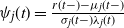$\psi_j(t)=\frac{r(t-)-\mu_j(t-)}{\sigma_j(t-)\lambda_j(t)}$ when $\lambda_j(t)\not=0$ (i.e. $J(t\!-\!)\not=e_j$ ). Furthermore, we assume that

\begin{align*}1+\psi_j(t)>0 \quad \mbox{for} \ j=1,\ldots,N,\end{align*}

which is equivalent to saying that the risk premium $\mu_j(t\!-\!)-r(t\!-\!)<\sigma_j(t\!-\!)\lambda_j(t)$ for $j=1,\ldots,N$ . Note that $\psi_0(t)$ and $\psi_j(t)$ $(\,j=1,\ldots,N)$ are all bounded. Then $\{L(t)\,:\,0\leq t\leq T\}$ is a nonnegative true martingale and $\mathbb{E}_{\mathbb{P}}[L(t)] = 1$ .

Let $\mathbb{Q}$ be the measure defined by the Radon–Nikodym derivative $\frac{\mathrm{d}\mathbb{Q}}{\mathrm{d}\mathbb{P}}|_{\mathcal{F}_t}=L(t)$ . Then under $\mathbb{Q}$ , $W^{\mathbb{Q}}(t)=W(t)-\int^t_0\psi_0(s)\mathrm{d}s$ is a standard $\mathbb{Q}$ -Brownian motion, and $\overline{\Phi}^{\mathbb{Q}}_j(t)=\Phi_j(t)-\int^t_0(1+\psi_j(s))\lambda_j(s)\mathrm{d}s$ is a martingale for $1\leq j\leq N$ . The discounted price processes for the securities described by

(2) \begin{align}\begin{cases}\mathrm{d}\tilde{S}_0(t)=\tilde S_0(t\!-\!)\biggl[ (\mu_0(t\!-\!)+\sigma_0(t\!-\!)\psi_0(t)-r(t\!-\!))\mathrm{d}t+\sigma_0(t)\mathrm{d}W^{\mathbb{Q}}(t)\\[10pt] \ \ \ \ \ \ \ \ \ \ \ \ \ +\int_{\mathbb{R}}\rho(t-,x)\overline\Pi(\mathrm{d}t,\mathrm{d}x)+\sum\limits^N_{i=1}\int_{\mathbb{R}}x\overline\Pi^i_U(\mathrm{d}t,\mathrm{d}x)\biggl],\\[10pt] \mathrm{d}\tilde S_j(t)=\tilde S_j(t\!-\!)\Big[ (\mu_j(t\!-\!)+\sigma_j(t\!-\!)\lambda_j(t)\psi_j(t)-r(t\!-\!))\mathrm{d}t+\sigma_j(t\!-\!)\mathrm{d}\overline{\Phi}^{\mathbb{Q}}_j(t)\Big],\\[10pt] \mathrm{d}\tilde S^{(k)}(t)=\tilde S^{(k)}(t\!-\!)\Big[ (\mu^{(k)}(t)-r(t))\mathrm{d}t+\sigma^{(k)}(t\!-\!)\mathrm{d}\overline{Z}^{(k)}(t)\Big],\\[10pt] \mathrm{d}\tilde S^{(l)}_i(t)=\tilde S^{(l)}_i(t\!-\!)\Big[ (\mu^{(l)}_i(t)-r(t))\mathrm{d}t+\sigma^{(l)}_i(t\!-\!)\mathrm{d}\overline{\Psi}^{(l)}_i(t)\Big]\\[10pt] \end{cases}\end{align}

for $i,j = 1,\ldots,N$ , $k\geq1$ , and $l \geq 1$ are martingales under $\mathbb{Q}$ . Then this market is asymptotic-arbitrage-free (see Proposition 6.1 in [Reference Björk and Näslund2]).

Let $L^2(\Omega,\mathcal{F}_T,\mathbb{Q})$ (abbreviated as $L^2(\mathbb{Q})$ ) be the set of measurable functions

\begin{align*}\left\{f\,:\,\Omega \rightarrow \mathbb{R};\ ||\,f||_2=\bigg(\int_{\Omega}|\,f|^2\mathrm{d}\mathbb{Q}\bigg)^{\frac{1}{2}}<\infty \right\}\!.\end{align*}

If we apply Theorem 9 in [Reference Palmowski, Stettner and Sulima24], the enlarged market is asymptotically complete; that is to say that for every square-integrable contingent claim A (i.e. a nonnegative square-integrable random variable in $L^2(\mathbb{Q})$ ) we can find a sequence of admissible strategies whose final values converge in $L^2(\mathbb{Q})$ to A.

The model setting described above aligns with that in [Reference Palmowski, Stettner and Sulima24], to which the reader is referred for more detailed information.

3. The Optimal Investment Problem

We consider an agent who invests his initial wealth in financial assets in our market in order to maximize the expected utility of the terminal wealth. We restrict ourselves to self-financing portfolio strategies:

\begin{align*}\big\{\pi(t)=\big(\pi_0(t),\pi_1(t),\ldots,\pi_N(t),\pi^{(1)}(t),\ldots,\pi^{(1)}_1(t),\ldots,\pi^{(1)}_N(t),\ldots\big), 0\leq t\leq T\big\},\end{align*}

where $\pi_0(t)$ represents the proportion of wealth invested in the stock, and $\pi_j(t)$ $(\,j=1,\ldots,N)$ , $\pi^{(k)}(t)$ $(k\geq 1)$ , and $\pi^{(l)}_i(t)$ $(i=1,\ldots,N, l\geq 1) $ represent the proportions of wealth invested in the jth geometric Markovian jump securities $S_j(t)$ , the Markovian power-jump securities $S^{(k)}(t)$ , and the impulse regime-switching securities $S^{(l)}_i(t)$ , respectively, so the proportion of wealth invested in the riskless security is $1-\sum\limits^N_{j=0}\pi_j(t)-\sum\limits^{\infty}_{k=1}\pi^{(k)}-\sum\limits^N_{i=1}\sum\limits^{\infty}_{l=1}\pi^{(l)}_i$ . They satisfy $\mathbb{P}$ -a.s.

\begin{align}&\int^T_0|\pi(t)|^2\mathrm{d}t<\infty, \nonumber\\&\int_{\mathbb{R}}(\pi_0(t)\rho(t-,x)+\sum\limits^{\infty}_{k=1}\pi^{(k)}(t)\sigma^{(k)}(t\!-\!)\rho^k(t-,x))\overline\Pi(\mathrm{d}t,\mathrm{d}x)<\infty, \nonumber\\&\int_{\mathbb{R}}\sum\limits^N_{i=1}(x\pi_0(t)+\sum\limits^{\infty}_{l=1}x^l\pi^{(l)}_i(t)\sigma^{(l)}_i(t\!-\!))\overline\Pi^i_U(\mathrm{d}t,\mathrm{d}x)<\infty.\nonumber\end{align}

We assume all the processes in $\{\pi(t)\}$ are predictable. Then the total wealth $\{X(t)\,:\,0\leq t\leq T\}$ associated with $\{\pi(t)\,:\,0\leq t\leq T\}$ can be expressed as

(3) \begin{equation}\begin{split}\mathrm{d}X_t=\ &X_{t-}\Bigg[\Bigg(1-\sum\limits^N_{j=0}\pi_j(t)-\sum\limits^{\infty}_{k=1}\pi^{(k)}(t)-\sum\limits^N_{i=1}\sum\limits^{\infty}_{l=1}\pi^{(l)}_i(t)\Bigg)\frac{\mathrm{d}B(t)}{B(t)}+\pi_0(t)\frac{\mathrm{d}S_0(t)}{S_0(t\!-\!)}\\[4pt]&+\sum\limits^N_{j=1}\pi_j(t)\frac{\mathrm{d}S_j(t)}{S_j(t\!-\!)}+\sum\limits^{\infty}_{k=1}\pi^{(k)}(t)\frac{\mathrm{d}S^{(k)}(t)}{S^{(k)}(t\!-\!)}+\sum\limits^N_{i=1}\sum\limits^{\infty}_{l=1}\pi^{(l)}_i(t)\frac{\mathrm{d}S^{(l)}_i(t)}{S^{(l)}_i(t\!-\!)}\Bigg].\end{split}\end{equation}

We investigate the optimization problem

(4) \begin{equation}\mathop{\arg\max}\limits_{X_T\in L^1(\mathbb{Q})}\bigg\{\mathbb{E}_{\mathbb{P}}\big[U(X_T)\big]\,:\,\mathbb{E}_{\mathbb{Q}}\bigg[\frac{X_T}{B(T)}\bigg]=x_0\bigg\},\end{equation}

where $U(\!\cdot\!)$ is a utility function, $x_0>0$ is the initial wealth, and $B(T)=e^{\int^T_0r(t)\mathrm{d}t}$ . If $X_T$ is a solution of (4), we say that it is the optimal terminal wealth. We solve this problem by the method of Lagrange multipliers,

\begin{align*}\mathop{\arg\max}\limits_{X_T\in L^1(\mathbb{Q})}\bigg\{\mathbb{E}_{\mathbb{P}}\big[U(X_T)\big]-\lambda_T\mathbb{E}_{\mathbb Q}\bigg[\frac{X_T}{B(T)}-x_0\bigg]\bigg\},\end{align*}

which is equivalent to

\begin{equation*}\mathop{\arg\max}\limits_{X_T\in L^1(\mathbb{Q})}\bigg\{\mathbb{E}_{\mathbb{P}}\bigg[U(X_T)-\lambda_T\bigg(\frac{\mathrm d\mathbb{Q}}{\mathrm d\mathbb{P}}\frac{X_T}{B(T)}-x_0\bigg)\bigg]\bigg\}.\end{equation*}

It is easy to get the optimal solution of (4) that satisfies the following first-order condition:

\begin{align*}U'(X_T)=\frac{\lambda_T}{B(T)}\frac{\mathrm d\mathbb{Q}}{\mathrm d\mathbb{P}}.\end{align*}

Then the optimal terminal wealth is given by

(5) \begin{equation}X_T=(U')^{-1}\bigg(\frac{\lambda_T}{B(T)}\frac{\mathrm d\mathbb{Q}}{\mathrm d\mathbb{P}}\bigg),\end{equation}

where $\lambda_T$ is the solution obtained by substitution of (5) into (4). That is, $\lambda_T$ satisfies the following equation,

(6) \begin{equation}\mathbb{E}_{\mathbb Q}\bigg[\frac{1}{B(T)}(U')^{-1}\bigg(\frac{\lambda_T}{B(T)}\frac{\mathrm d\mathbb{Q}}{\mathrm d\mathbb{P}}\bigg)\bigg]=x_0.\end{equation}

We cannot derive the explicit solution unless the market has better properties, but for a kind of special utility, i.e. the HARA utility function, we can give the closed-form solution, see, for example [Reference Merton19]. So we will investigate the HARA utility function

(7) \begin{equation}U_{\mathrm{H}}(x)=\frac{1-\gamma}{\beta\gamma}\left(\frac{\beta x}{1-\gamma}+\eta\right)^{\gamma},\ \ \ x \in \left(-\frac{\eta(1-\gamma)}{\beta},+\infty\right)\!,\end{equation}

where $\beta >0$ , $\eta >0$ , and $\gamma \in \mathbb{R}\setminus\{0,1\}$ . For rational investment, we apply the limit $\gamma<1$ . The HARA utility function has very good properties:

1. (i) When $\eta = 1$ , $\gamma \to -\infty$ , $U_{\mathrm{H}}(x)$ converges to the exponential utility function

   (8) \begin{equation}U_{\mathrm{e}}(x)=-\frac{1}{\beta}e^{-\beta x},\ \ \ x\in(\!-\infty,+\infty).\end{equation}

2. (ii) When $\gamma \to 0$ , the modified HARA function

   \begin{align*}U_{\mathrm{mH}}(x)=\frac{1-\gamma}{\beta\gamma}\bigg[\bigg(\frac{\beta x}{1-\gamma}+\eta\bigg)^{\gamma}-1\bigg], \end{align*}

which has the same solution as (7) when the optimal problem (4) is computed, converges to the extended logarithmic utility function

(9) \begin{equation}U_{\mathrm{l}}(x)=\frac{1}{\beta}\log(\beta x+\eta),\ \ \ x\in\bigg(-\frac{\eta}{\beta},+\infty\bigg).\end{equation}

In this section, we apply the martingale method to solve the optimal investment problem of maximizing the expected utility of the terminal wealth in a continuous-time Itô–Markov additive market. We will solve this problem in two steps: first, we will get the optimal wealth processes and, second, we will get the optimal hedging portfolio strategies that replicate the wealth processes.

3.1. Optimal wealth process

In this section, we apply the martingale method to solve the optimal investment problem of maximizing the expected utility of the terminal wealth. First, we give a very useful lemma that will be frequently used in this article. Remember the two probability measures $\mathbb{P}$ and $\mathbb{Q}$ with the Radon–Nikodym derivative $\frac{\mathrm{d}\mathbb{Q}}{\mathrm{d}\mathbb{P}}|_{\mathcal{F}_t}=L(t)$ .

Lemma 1. A process $\{Z_t, t\in [0,T]\}$ is a $\mathbb{Q}$ -martingale if and only if $\{Z_tL(t)\,:\,t\in [0,T]\}$ is a $\mathbb{P}$ -martingale.

Take $X_T=(U')^{-1}\big(\frac{\lambda_T}{B(T)}\frac{\mathrm d\mathbb{Q}}{\mathrm d\mathbb{P}}\big)$ , which satisfies (6) as a contingent claim in the option pricing, Then 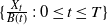$\{\frac{X_t}{B(t)}\,:\,0\leq t\leq T\}$ is a $\mathbb{Q}$ -martingale. From Lemma 1 we can get the optimal wealth process for a realistic measure ( $\mathbb{P}$ ) at a given time $t \in [0,T]$ :

(10) \begin{equation}X_t=B(t)\mathbb{E}_{\mathbb{Q}}\bigg[\frac{X_T}{B(T)}\bigg|\mathcal F_t\bigg]=\frac{B(t)}{L(t)}\mathbb{E}_{\mathbb{P}}\bigg[X_T\frac{L(T)}{B(T)}\bigg|\mathcal F_t\bigg].\end{equation}

Note that for any $\alpha$ and $0\leq t \leq T$ ,

(11) \begin{align}&\mathbb{E}_{\mathbb{P}}\Bigg[\exp\left(\int^t_0\psi_0(s)\mathrm{d}W(s)\right)^{\alpha}\times\prod^N_{j=1}\prod_{\substack{0 < s\leq t\nonumber\\J(s-)\neq J(s)\\J(s)=\mathbf{e}_j}}(1+\psi_j(s))^{\alpha}\Bigg]\\ &\quad\quad =\exp\left(\frac{1}{2}\int^t_0 \alpha^2\psi_0^2(s)\mathrm{d}s+\sum\limits^N_{j=1}\int^t_0((1+\psi_j(s))^\alpha-1)\phi_j(\mathrm{d}s)\right)\!,\end{align}

which means $(L(t))^{\alpha}$ is integrable since $\psi_0$ and $\psi_j$ $(\,j=1,2,\ldots,N)$ take only finitely many values. Next we give the optimal wealth process for each of the three utility functions.

Proposition 2. Under HARA utility, the optimal wealth process at time $t\in[0,T]$ is expressed as

(12) \begin{equation}X_t^{\mathrm{H}}\,:\!=\,\frac{B(t)}{L(t)}P(\gamma, \eta)\mathbb{E}_{\mathbb{P}}\bigg[\Big(\frac{L(T)}{B(T)}\Big)^{\frac{\gamma}{\gamma-1}}\bigg|\mathcal{F}_t\bigg]-\frac{B(t)}{L(t)}\frac{(1-\gamma)\eta}{\beta }\mathbb{E}_{\mathbb{P}}\left[\frac{L(T)}{B(T)}\bigg|\mathcal{F}_t\right]\!,\end{equation}

where $P(\gamma, \eta) = \big(x_0+\frac{\eta(1-\gamma)}{\beta }\mathbb{E}_{\mathbb{P}}\big[\frac{L(T)}{B(T)}\big]\big)\big(\mathbb{E}_{\mathbb{P}}\big[\frac{L(T)}{B(T)}\big]^{\frac{\gamma}{\gamma-1}}\big)^{-1}$ .

Proof. From (7) and (6), we get

\begin{align}\lambda_T&=\bigg(\frac{x_0\beta}{1-\gamma}+\eta \mathbb{E}_{\mathbb{P}}\bigg[\frac{L(T)}{B(T)}\bigg]\bigg)^{\gamma-1}\bigg(\mathbb{E}_{\mathbb{P}}\bigg[\frac{L(T)}{B(T)}\bigg]^{\frac{\gamma}{\gamma-1}}\bigg)^{1-\gamma}.\nonumber\end{align}

By substituting the above result into (5), we get

\begin{align}X_T^{\mathrm{H}}&=(U_{\mathrm{H}}')^{-1}\bigg(\frac{\lambda_T}{B(T)}\frac{\mathrm d\mathbb{Q}}{\mathrm d\mathbb{P}}\bigg)\nonumber\\[4pt]&=\frac{1-\gamma}{\beta}\bigg[\bigg(\frac{\lambda_T}{B(T)}L(T)\bigg)^{\frac{1}{\gamma-1}}-\eta\bigg]\nonumber\\[4pt]&=\bigg(x_0+\frac{\eta(1-\gamma)}{\beta }\mathbb{E}_{\mathbb{P}}\bigg[\frac{L(T)}{B(T)}\bigg]\bigg)\bigg(\mathbb{E}_{\mathbb{P}}\bigg[\frac{L(T)}{B(T)}\bigg]^{\frac{\gamma}{\gamma-1}}\bigg)^{-1}\bigg(\frac{L(T)}{B(T)}\bigg)^{\frac{1}{\gamma-1}}-\frac{(1-\gamma)\eta}{\beta}\nonumber\\[4pt]&=P(\gamma, \eta)\bigg(\frac{L(T)}{B(T)}\bigg)^{\frac{1}{\gamma-1}}-\frac{(1-\gamma)\eta}{\beta}.\nonumber\end{align}

Then by (10) and (11), we get the desired result.

Proposition 3. For exponential utility, the optimal wealth process at time $t\in[0,T]$ is expressed as

\begin{equation*}X_t^{\mathrm{e}}\,:\!=\,K\frac{B(t)}{L(t)}\mathbb{E}_{\mathbb{P}}\bigg[\frac{L(T)}{B(T)}\bigg|\mathcal{F}_t\bigg] -\frac{B(t)}{\beta L(t)}\mathbb{E}_{\mathbb{P}}\bigg[\frac{L(T)}{B(T)}\log\bigg(\frac{L(T)}{B(T)}\bigg)\bigg|\mathcal{F}_t\bigg],\end{equation*}

where $K = \big(x_0+\frac{1}{\beta}\mathbb{E}_{\mathbb{P}}\big[\frac{L(T)}{B(T)}\log\big(\frac{L(T)}{B(T)}\big)\big]\big)(\mathbb{E}_{\mathbb{P}}\big[\frac{L(T)}{B(T)}])^{-1}$ .

Proposition 4. Under extended logarithmic utility, the optimal wealth process at time $t\in[0,T]$ is expressed as

(13) \begin{equation}X_t^{\mathrm{l}}\,:\!=\,M(\eta,\beta)\frac{B(t)}{L(t)}-\frac{\eta}{\beta}\frac{B(t)}{L(t)}\mathbb{E}_{\mathbb{P}}\bigg[\frac{L(T)}{B(T)}\bigg|\mathcal{F}_t\bigg],\end{equation}

where $M(\eta,\beta)=x_0+\frac{\eta}{\beta}\mathbb{E}_{\mathbb{P}}[\frac{L(T)}{B(T)}]$ is a constant.

3.2. Optimal portfolio strategy

In this subsection, we give the explicit optimal porfolios for HARA, exponential, and extended logarithmic utility, respectively, which depend essentially on L(t). Note that Itô’s formula for semimartingales will be frequently used in the proof of the following result; for more details we refer the reader to [Reference Ikeda and Watanabe14].

By using the expressions for L(t) and X(t)—(1) and (3), respectively—and Itô’s formula for semimartingales, we have

(14) \begin{align}\begin{split}&\mathrm{d}\bigg(X_t\frac{L(t)}{B(t)}\bigg)\\&=\ X_{t-}\frac{L(t\!-\!)}{B(t)}\Bigg\{\big(\pi_0(t)\sigma_0(t)+\psi_0(t)\big)\mathrm{d}W(t)+\sum\limits^N_{j=1}\big[\pi_j(t)\sigma_j(t\!-\!)\big(1+\psi_j(t)\big)+\psi_j(t)\big]\mathrm{d}\overline\Phi_j(t)\\&\quad +\big(\pi_0(t)+\pi^{(1)}(t)\sigma^{(1)}(t\!-\!)\big)\int_{\mathbb{R}}\rho(t-,x)\overline\Pi(\mathrm{d}t,\mathrm{d}x)+\sum\limits^{\infty}_{k=2}\pi^{(k)}(t)\sigma^{(k)}(t\!-\!)\mathrm{d}\overline Z^{(k)}(t)\\&\quad +\sum^N_{i=1}\big(\pi_0(t)+\pi_i^{(1)}(t)\sigma^{(1)}_i(t\!-\!)\big)\int_{\mathbb{R}}x\overline \Pi^i_U(\mathrm{d}t,\mathrm{d}x)+\sum\limits^N_{i=1}\sum\limits^{\infty}_{l=2}\pi^{(l)}_i(t)\sigma^{(l)}_i(t\!-\!)\mathrm{d}\overline\Psi^{(l)}_i(t)\Bigg\}.\end{split}\end{align}

Theorem 1. The optimal portfolio strategy at time $t\in[0,T]$ for the HARA utility, which we denote by $\{\pi^{\mathrm{H}}(t)\}$ , is given by the following formulas:

\begin{equation}\begin{split} \nonumber\pi_0^{\mathrm{H}}(t)&=\frac{\psi_0(t)}{X_{t}^{\mathrm{H}} \sigma_0(t)}\bigg[\frac{\gamma}{\gamma-1}P(\gamma, \eta)\bigg(\frac{L(t)}{B(t)}\bigg)^{\frac{1}{\gamma-1}}\zeta_{\frac{\gamma}{\gamma-1}}(J(t)) -\frac{(1-\gamma)\eta}{\beta }\zeta_1(J(t))\bigg]-\frac{\psi_0(t)}{\sigma_0(t)},\\\end{split}\end{equation}

(15) \begin{equation}\begin{split}\pi_j^{\mathrm{H}}(t)&=\frac{1}{X^{\mathrm{H}}_{t-}\sigma_j(t\!-\!)\big(1+\psi_j(t)\big)}\Bigg\{P(\gamma,\eta)\bigg(\frac{L(t)}{B(t)}\bigg)^{\frac{1}{\gamma-1}}\Big[\zeta_{\frac{\gamma}{\gamma-1}}(J(t\!-\!))((1+\psi_j(t))^{\frac{\gamma}{\gamma-1}}-1)\\&\,\,\,+(\zeta_{\frac{\gamma}{\gamma-1}}(\,j)-\zeta_{\frac{\gamma}{\gamma-1}}(J(t\!-\!)))(1+\psi_j(t))^{\frac{\gamma}{\gamma-1}}\Big]\\&\,\,\,-\frac{(1-\gamma)\eta}{\beta }\big[\zeta_1(J(t))\psi_j(t)+(1+\psi_j(t))(\zeta_1(\,j)-\zeta_1(J(t\!-\!)))\big]\Bigg\}\\&\,\,\,-\frac{\psi_j(t)}{\sigma_j(t\!-\!)\big(1+\psi_j(t)\big)},\\\pi^{\mathrm{H},(1)}(t)&=-\frac{\pi^{\mathrm{H}}_0(t)}{\sigma^{(1)}(t\!-\!)},\\\pi^{\mathrm{H},(1)}_i(t)&=-\frac{\pi^{\mathrm{H}}_0(t)}{\sigma^{(1)}_i(t\!-\!)}\quad \mbox{for} \ i,j=1,\ldots,N,\\\pi^{\mathrm{H},(k)}(t)&=0, \pi^{\mathrm{H},(l)}_i(t)(t)=0 \quad \mbox{for} \ k\geq 2,\ l\geq 2,\ i=1,\ldots,N,\end{split}\end{equation}

where $\zeta_\alpha(x)\,:\!=\,\mathbb{E}_{\mathbb{P}}\big[\big(\frac{L(T,t)}{B(T,t)}\big)^{\alpha}|J(t)\big]|_{J(t)=x}$ depends only on J(t).

Proof. Note that, from (12) and by using Itô’s formula, we have

\begin{equation*}\begin{split}\mathrm{d}\bigg(X_t^{\mathrm{H}}\frac{L(t)}{B(t)}\bigg)=P(\gamma, \eta)\mathrm{d}\mathbb{E}_{\mathbb{P}}\bigg[\bigg(\frac{L(T)}{B(T)}\bigg)^{\frac{\gamma}{\gamma-1}}\bigg|\mathcal{F}_t\bigg]-\frac{(1-\gamma)\eta}{\beta }\mathrm{d}\left(\mathbb{E}_{\mathbb{P}}\bigg[\frac{L(T)}{B(T)}|\mathcal{F}_t\bigg]\right).\end{split}\end{equation*}

It is easy to show that $\mathbb{E}_{\mathbb{P}}\bigg[\big(\frac{L(T)}{B(T)}\big)^{\frac{\gamma}{\gamma-1}}\bigg|\mathcal{F}_t\bigg]$ is a martingale and is square-integrable. By Jensen’s inequality,

\begin{align*}&\mathbb{E}_{\mathbb{P}}\bigg[\bigg(\mathbb{E}_{\mathbb{P}}\bigg[\bigg(\frac{L(T)}{B(T)}\bigg)^{\frac{\gamma}{\gamma-1}}|\mathcal{F}_t\bigg]\bigg)^2\bigg]\leq \mathbb{E}_{\mathbb{P}}\bigg[\mathbb{E}_{\mathbb{P}}\bigg[\bigg(\frac{L(T)}{B(T)}\bigg)^{\frac{2\gamma}{\gamma-1}}|\mathcal{F}_t\bigg]\bigg]=\mathbb{E}_{\mathbb{P}}\bigg[\bigg(\frac{L(T)}{B(T)}\bigg)^{\frac{2\gamma}{\gamma-1}}\bigg]\\[3pt]\nonumber&\quad =\mathbb{E}_{\mathbb{P}}\bigg[\exp\bigg\{-\frac{2\gamma}{\gamma-1}\int^t_0r(s)\mathrm{d}s+\frac{\gamma^2+\gamma}{(\gamma-1)^2}\int^t_0\psi_0^2(s)\mathrm{d}s\\[3pt]\nonumber&\quad\quad +\sum^N_{j=1}\int^t_0\big((1+\psi_j(s))^{\frac{2\gamma}{\gamma-1}}-1-\frac{2\gamma}{\gamma-1}\psi_j(s)\big)\lambda_j(s)\mathrm{d}s\bigg\}\bigg]<\infty,\end{align*}

since r(t), $\psi_0(t)$ , and $\psi_j(t), j=1,2,\ldots, N$ , take only finitely many values. Let $L(T,t)\,:\!=\,\frac{L(T)}{L(t)}$ and 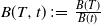$B(T,t)\,:\!=\,\frac{B(T)}{B(t)}$ . Using the Markov property of $\{J(t)\,:\,0\leq t\leq T\}$ and independent increment of Brownian motion $\{W(t)\,:\,t\geq 0\}$ , we have

\begin{align*}\mathbb{E}_{\mathbb{P}}\bigg[\bigg(\frac{L(T,t)}{B(T,t)}\bigg)^{\frac{\gamma}{\gamma-1}}\bigg|\mathcal{F}_t\bigg] =\mathbb{E}_{\mathbb{P}}\bigg[\bigg(\frac{L(T,t)}{B(T,t)}\bigg)^{\frac{\gamma}{\gamma-1}}\bigg|J(t)\bigg]=\zeta_\frac{\gamma}{\gamma-1}(J(t)),\end{align*}

where $\zeta_\alpha(x)\,:\!=\,\mathbb{E}_{\mathbb{P}}\big[\big(\frac{L(T,t)}{B(T,t)}\big)^{\alpha}|J(t)\big]|_{J(t)=x}$ depends only on J(t). Then

\begin{align*}\mathbb{E}_{\mathbb{P}}\bigg[\bigg(\frac{L(T)}{B(T)}\bigg)^{\frac{\gamma}{\gamma-1}}\bigg|\mathcal{F}_t\bigg]=\bigg(\frac{L(t)}{B(t)}\bigg)^{\frac{\gamma}{\gamma-1}}\zeta_{\frac{\gamma}{\gamma-1}}(J(t)),\end{align*}

and similarly $\mathbb{E}_{\mathbb{P}}\big[\frac{L(T)}{B(T)}|\mathcal{F}_t\big]=\frac{L(t)}{B(t)}\zeta_1(J(t))$ . Let $Y(t)=\frac{L(t)}{B(t)}$ . Then

\begin{align*} \mathrm{d}Y(t)=Y(t\!-\!)\bigg(-r(t)\mathrm{d}t+\psi_0(t)\mathrm{d}W(t)+\sum^N_{j=1}\psi_j(t)\mathrm{d}\overline\Phi_j(t)\bigg),\end{align*}

and then

\begin{align}\nonumber\mathrm{d}(Y(t))^{\frac{\gamma}{\gamma-1}}&=(Y(t\!-\!))^{\frac{\gamma}{\gamma-1}}\bigg[\frac{\gamma}{\gamma-1}(-r(t)\mathrm{d}t+\psi_0(t)\mathrm{d}W(t))+\frac{1}{2}\frac{\gamma}{(\gamma-1)^2}\psi^2_0(t)\mathrm{d}t\\ \nonumber&\quad +\sum^N_{j=1}\bigg((1+\psi_j(t))^{\frac{\gamma}{\gamma-1}}-1\bigg)\mathrm{d}\overline\Phi_j(t) \\ \nonumber&\quad +\sum^N_{j=1}\bigg((1+\psi_j(t))^{\frac{\gamma}{\gamma-1}}-1-\frac{\gamma}{\gamma-1}\psi_j(t)\bigg)\lambda_j(t)\mathrm{d}t\bigg].\end{align}

Therefore, using the martingale property of $(Y(t))^{\frac{\gamma}{\gamma-1}}\zeta_{\frac{\gamma}{\gamma-1}}(J(t))$ , we have

\begin{align*}\nonumber\mathrm{d}\bigg((Y(t))^{\frac{\gamma}{\gamma-1}}\zeta_{\frac{\gamma}{\gamma-1}}(J(t))\bigg)&=(Y(t\!-\!))^{\frac{\gamma}{\gamma-1}}\bigg\{\frac{\gamma}{\gamma-1}\zeta_{\frac{\gamma}{\gamma-1}}(J(t\!-\!))\psi_0(t)\mathrm{d}W(t)\\ \nonumber&\quad +\sum^N_{j=1}\big[\zeta_{\frac{\gamma}{\gamma-1}}(J(t\!-\!))((1+\psi_j(t))^{\frac{\gamma}{\gamma-1}}-1)\\ &\quad+(1+\psi_j(t))^{\frac{\gamma}{\gamma-1}}(\zeta_{\frac{\gamma}{\gamma-1}}(\,j)-\zeta_{\frac{\gamma}{\gamma-1}}(J(t\!-\!)))\big]\mathrm{d}\overline\Phi_j(t)\bigg\},\end{align*}

and similarly we can get $\mathrm{d}(Y(t)\zeta_1(J(t)))$ . Combining all the above results, we get

\begin{align}\nonumber \mathrm{d}\bigg(X_t^{\mathrm{H}}\frac{L(t)}{B(t)}\bigg)&=P(\gamma, \eta)\mathrm{d}\bigg(\mathbb{E}_{\mathbb{P}}\bigg[\bigg(\frac{L(T)}{B(T)}\bigg)^{\frac{\gamma}{\gamma-1}}\bigg|\mathcal{F}_t\bigg]\bigg)-\frac{(1-\gamma)\eta}{\beta }\mathrm{d}\left(\mathbb{E}_{\mathbb{P}}\bigg[\frac{L(T)}{B(T)}\bigg|\mathcal{F}_t\bigg]\right)\\[5pt] \nonumber&=P(\gamma, \eta)\mathrm{d}\bigg(\bigg(\frac{L(t)}{B(t)}\bigg)^{\frac{\gamma}{\gamma-1}}\mathbb{E}_{\mathbb{P}}\bigg[\bigg(\frac{L(T,t)}{B(T,t)}\bigg)^{\frac{\gamma}{\gamma-1}}\bigg|\mathcal{F}_t\bigg]\bigg)-\frac{(1-\gamma)\eta}{\beta }\mathrm{d}\mathbb{E}_{\mathbb{P}}\bigg[\frac{L(T)}{B(T)}\bigg|\mathcal{F}_t\bigg] \\[5pt] \nonumber&=P(\gamma,\eta)\mathrm{d}\bigg(\bigg(\frac{L(t)}{B(t)}\bigg)^{\frac{\gamma}{\gamma-1}}\zeta_{\frac{\gamma}{\gamma-1}}(J(t))\bigg)-\frac{(1-\gamma)\eta}{\beta}\mathrm{d}\bigg(\frac{L(t)}{B(t)}\zeta_1(J(t))\bigg) \\[5pt] \nonumber&=\bigg[\frac{\gamma}{\gamma-1}P(\gamma,\eta)\bigg(\frac{L(t)}{B(t)}\bigg)^{\frac{\gamma}{\gamma-1}}\zeta_{\frac{\gamma}{\gamma-1}}(J(t))-\frac{(1-\gamma)\eta}{\beta}\frac{L(t)}{B(t)}\zeta_1(J(t))\bigg]\psi_0(t)\mathrm{d}W(t)\\[5pt] \nonumber &\quad +\sum^N_{j=1}\bigg\{P(\gamma,\eta)\bigg(\frac{L(t)}{B(t)}\bigg)^{\frac{\gamma}{\gamma-1}}\big[\zeta_{\frac{\gamma}{\gamma-1}}(J(t\!-\!))((1+\psi_j(t))^{\frac{\gamma}{\gamma-1}}-1)\\[5pt] \nonumber&\quad +(1+\psi_j(t))^{\frac{\gamma}{\gamma-1}}(\zeta_{\frac{\gamma}{\gamma-1}}(\,j)-\zeta_{\frac{\gamma}{\gamma-1}}(J(t\!-\!))\big]\\[5pt] \nonumber&\quad -\frac{(1-\gamma)\eta}{\beta }\frac{L(t)}{B(t)}\big[\zeta_1(J(t\!-\!))\psi_j(t)+(\zeta_1(\,j)-\zeta_1(J(t\!-\!)))(1+\psi_j(t))\big]\bigg\}\mathrm{d}\overline\Phi_j(t).\end{align}

By comparing this with (14), we can get $\{\pi^{\mathrm{H}}(t)\}$ .

Theorem 2. The optimal portfolio strategy at time $t\in[0,T]$ for the exponential utility, which we denote by $\{\pi^{\mathrm{e}}(t)\}$ , is given by the following formulas:

(16) \begin{equation}\begin{split}&\pi_0^{\mathrm{e}}(t)=\frac{\psi_0(t)}{X^{\mathrm{e}}_{t}\sigma_0(t)}\bigg[\bigg(K-\frac{1}{\beta}\bigg(1+\log\frac{L(t)}{B(t)}\bigg)\bigg)\zeta_1(J(t))-\frac{1}{\beta}\xi(J(t))\bigg]-\frac{\psi_0(t)}{\sigma_0(t)},\\[5pt]&\pi_j^{\mathrm{e}}(t)=\frac{1}{X^{\mathrm{e}}_{t-}\sigma_j(t\!-\!)}\bigg\{(\zeta_1(\,j)-\zeta_1(J(t\!-\!)))\bigg[K-\frac{1}{\beta}\log\frac{L(t\!-\!)}{B(t\!-\!)}+\psi_j(t)\bigg]-\frac{1}{\beta}\zeta_1(J(t\!-\!))\psi_j(t)\\[5pt]&\ \ \ \ \ \ \ \ \ \ \ \ \ \ \ \ \ -\frac{1}{\beta}(\xi(\,j)-\xi(J(t\!-\!))) +\bigg[\zeta_1(J(t\!-\!))\bigg(K-\frac{1}{\beta}\log\frac{L(t\!-\!)}{B(t\!-\!)}\bigg) -\frac{1}{\beta}\xi(J(t\!-\!))\bigg]\frac{\psi_j(t)}{1+\psi_j(t)}\bigg\}\\[5pt]& \ \ \ \ \ \ \ \ \ \ \ \ \ \ \ \ \ -\frac{\psi_j(t)}{\sigma_j(t\!-\!)(1+\psi_j(t))},\\[5pt]&\pi^{\mathrm{e},(1)}(t)=-\frac{\pi^{\mathrm{e}}_0(t)}{\sigma^{(1)}(t\!-\!)},\\[5pt]&\pi^{\mathrm{e},(1)}_i(t)= -\frac{\pi^{\mathrm{e}}_0(t)}{\sigma^{(1)}_i(t\!-\!)} \quad \mbox{for} \ i,j=1,\ldots,N,\\[5pt]&\pi^{\mathrm{e},(k)}(t)=0, \pi^{e,(l)}_i(t)(t)=0 \quad \mbox{for} \ k\geq 2,\ l\geq 2,\ i=1,\ldots,N,\end{split}\end{equation}

where $\xi(x)\,:\!=\,\mathbb{E}_{\mathbb{P}}\big[\frac{L(T,t)}{B(T,t)}\log\frac{L(T,t)}{B(T,t)}|J_t\big]|_{J_t=x}$ depends only on J(t) and $\zeta_1$ has been defined in Theorem 1.

Theorem 3. The optimal portfolio strategy at time $t\in[0,T]$ for the extended logarithmic utility, which we denote by $\{\pi^{\mathrm{l}}(t)\}$ , is given by the following formulas:

(17) \begin{equation}\begin{split}&\pi_0^{\mathrm{l}}(t)=-\frac{\psi_0(t)}{\sigma_0(t)}\bigg(1+\frac{\eta \zeta_1(J(t))}{\beta X_t^{\mathrm{l}}}\bigg), \\[4pt]&\pi_j^{\mathrm{l}}(t)=-\frac{\eta[\zeta_1(J(t))\psi_j(t)+(1+\psi_j(t))(\zeta_1(\,j)-\zeta_1(J(t\!-\!)))]}{\beta X_{t-}^{\mathrm{l}}\sigma_j(t\!-\!)(1+\psi_j(t))}-\frac{\psi_j(t)}{\sigma_j(t\!-\!)(1+\psi_j(t))},\\[4pt]&\pi^{\mathrm{l},(1)}(t)=-\frac{\pi^{\mathrm{l}}_0(t)}{\sigma^{(1)}(t\!-\!)},\\[4pt]&\pi^{\mathrm{l},(1)}_i(t)=-\frac{\pi^{\mathrm{l}}_0(t)}{\sigma^{(1)}_i(t\!-\!)}\quad \mbox{for} \ i,j=1,\ldots,N,\\[4pt]&\pi^{\mathrm{l},(k)}(t)=0, \pi^{l,(l)}_i(t)(t)=0 \quad \mbox{for} \ k\geq 2,\ l\geq 2,\ i=1,\ldots,N.\end{split}\end{equation}

4. Weak Convergence Results

We know from (7), (8), and (9) that the HARA utility function converges to the other two utility functions when parameters vary in a suitable way. Do the corresponding optimal investment strategies converge? Niu [Reference Niu21] gave the weak convergence results for the optimal wealth processes and strategies in a simple Lévy market. In this section, we prove that the weak convergence results still hold in the Itô–Markov additive market, although the proof is some more complicated.

First, we give a result similar to the results given in [Reference Grasselli10, Reference Niu21].

Proposition 5. For each $t \in [0,T]$ ,

(18) \begin{align}&\lim_{\substack{\gamma \to -\infty\\\eta = 1}} X^{\mathrm{H}}_t = X^{\mathrm{e}}_t,\ \ \mathbb{P}\text{-a.s.},\end{align}

(19) \begin{align}&\lim_{\substack{\gamma \to -\infty\\\eta = 1}}\pi^{\mathrm{H}}(t)= \pi^{\mathrm{e}}(t),\ \ \mathbb{P}\text{-a.s.},\end{align}

(20) \begin{align}&\lim_{\gamma \to 0}X^{\mathrm{H}}_t= X^{\mathrm{l}}_t,\ \ \mathbb{P}\text{-a.s.},\end{align}

(21) \begin{align}&\lim_{\gamma \to 0}\pi^{\mathrm{H}}(t)= \pi^{\mathrm{l}}(t),\ \ \mathbb{P}\text{-a.s.}\end{align}

Before proving weak convergence results as a whole process, we make some preparations.

Proposition 6. For any finite set $\{t_1,\ldots,t_n\} \subset [0,T]$ ,

\begin{align*} (X^{\mathrm{H}}_{t_1},\ldots,X^{\mathrm{H}}_{t_n}) \Rightarrow (X^{\mathrm{e}}_{t_1},\ldots,X^{\mathrm{e}}_{t_n}),\ \ \ \gamma \to -\infty, \end{align*}

where $\Rightarrow$ means weak convergence.

Proof. For any finite set $\{t_1,\ldots,t_n\} \subset [0,T]$ and any finite set $\{u_1,\ldots,u_n\} \subset (0,\infty)$ , by (18) and the dominated convergence theorem, we have the convergence of the corresponding characteristic functions:

\begin{align*}\lim_{\gamma\to -\infty} \mathbb{E}_{\mathbb{P}}\bigg[\exp\bigg\{\!-i\sum^n_{k=1}u_kX^{\mathrm{H}}_{t_k}\bigg\}\bigg]&=\ \mathbb{E}_{\mathbb{P}}\bigg[\lim_{\gamma\to -\infty} \exp\bigg\{\!-i\sum^n_{k=1}u_kX^{\mathrm{H}}_{t_k}\bigg\}\bigg]\\&=\ \mathbb{E}_{\mathbb{P}}\bigg[\exp\bigg\{\!-i\sum^n_{k=1}u_kX^{\mathrm{e}}_{t_k}\bigg\}\bigg]\nonumber.\end{align*}

Let $D_{\mathbb{R}}[0,\infty)$ = $\{\,f\,:\,[0,\infty)\rightarrow\mathbb{R}, \mathrm{c}\acute{\mathrm{a}}\mathrm{dl}\grave{\mathrm{a}}\mathrm{g}\}$ . Then $X^{\mathrm{H}}(\!\cdot\!)$ , $X^{\mathrm{e}}(\!\cdot\!)$ , and $X^{\mathrm{l}}(\!\cdot\!)$ can be seen as stochastic processes in $D_{\mathbb{R}}[0,\infty)$ by extended $X^{\mathrm{H}}(t)=X^{\mathrm{H}}(T)$ , $X^{\mathrm{e}}(t)=X^{\mathrm{e}}(T)$ , and $X^{\mathrm{l}}(T)=X^{\mathrm{l}}(T)$ , respectively, for $t \in (T,\infty)$ .

Proof. Let $\{\tau_n\}$ be a sequence of stopping times bounded above by T, $t_n \rightarrow 0$ as $n \rightarrow \infty$ . We know from the criterion in [Reference Aldous1] that to get the tightness of $\{X^{\mathrm{H}}_n(\!\cdot\! )\}$ , we need to show that

(22) \begin{equation}X_n^{\mathrm{H}}(\tau_n+t_n)-X_n^{\mathrm{H}}(\tau_n)\xrightarrow{\mathbb{P}}0\quad \mbox{as} \ n\rightarrow \infty,\end{equation}

and $\{X^{\mathrm{H}}_n(t)\}$ is tight for each t, $0\leq t\leq T $ . The latter follows from Proposition 6 immediately, and we need only to show (22). We know from (10) that

\begin{align} X_n^{\mathrm{H}}(t)=\frac{B(t)}{L(t)} \mathbb{E}_{\mathbb{P}}\bigg[X_n^{\mathrm{H}}(T)\frac{L(T)}{B(T)}|\mathcal{F}_t\bigg],\,0\leq t\leq T.\nonumber\end{align}

To give a martingale representation of $\mathbb{E}_{\mathbb{P}}\big[X_n^{\mathrm{H}}(T)\frac{L(T)}{B(T)}|\mathcal{F}_{t}\big]$ , we first need to show that, by Jensen’s inequality,

\begin{align}\nonumber&\mathbb{E}_{\mathbb{P}}\bigg[\bigg(\mathbb{E}_{\mathbb{P}}\bigg[X_n^{\mathrm{H}}(T)\frac{L(T)}{B(T)}|\mathcal{F}_{t}\bigg]\bigg)^2\bigg]\\[3pt] \nonumber&\leq \mathbb{E}_{\mathbb{P}}\bigg[\mathbb{E}_{\mathbb{P}}\bigg[\bigg(X_n^{\mathrm{H}}(T)\frac{L(T)}{B(T)}\bigg)^2|\mathcal{F}_{t}\bigg]\bigg]=\mathbb{E}_{\mathbb{P}}\bigg[\bigg(X_n^{\mathrm{H}}(T)\frac{L(T)}{B(T)}\bigg)^2\bigg]\\[3pt]\nonumber&=\mathbb{E}_{\mathbb{P}}\bigg[\bigg(\!\bigg(x_0+\frac{(1-\gamma_n)\eta}{\beta }\mathbb{E}_{\mathbb{P}}\bigg[\frac{L(T)}{B(T)}\bigg]\bigg)\bigg(\mathbb{E}_{\mathbb{P}}\bigg[\frac{L(T)}{B(T)}\bigg]^{\frac{\gamma_n}{\gamma_n-1}}\bigg)^{-1}\!\bigg(\frac{L(T)}{B(T)}\bigg)^\frac{1}{\gamma_n-1}\!-\frac{(1-\gamma_n)\eta}{\beta}\bigg)^2\!\frac{L(T)^2}{B(T)^2}\bigg]\\[3pt] \nonumber&\rightarrow\bigg(x_0 \bigg(\mathbb{E}_{\mathbb{P}}\bigg[\frac{L(T)}{B(T)}\bigg]\bigg)^{-1}\bigg)^2\mathbb{E}_{\mathbb{P}}\bigg[\frac{L(T)^2}{B(T)^2}\bigg]<\infty\quad \mbox{as} \ n\rightarrow \infty.\end{align}

Then for each n, there exist predictable processes $g_{0,n}$ , $g_{\phi,n}^{(j)}$ that satisfy $\mathbb{E}_{\mathbb{P}}[\int^{T}_0g_{0,n}^2(s)\mathrm{d}s]<\infty$ and $\mathbb{E}_{\mathbb{P}}[\int^{T}_0(g_{\phi,n}^{(j)})^2(s)\mathrm{d}s]<\infty$ (for $j=1,\ldots,N$ ) such that

\begin{align*} \mathbb{E}_{\mathbb{P}}\bigg[X_n^{\mathrm{H}}(T)\frac{L(T)}{B(T)}|\mathcal{F}_{t}\bigg] = \mathbb{E}_{\mathbb{P}}\bigg[X_n^{\mathrm{H}}(T)\frac{L(T)}{B(T)}\bigg] + \int^t_0g_{0,n}(s)\mathrm{d}W(s)+\sum^N_{j=1}\int^t_0g_{\phi,n}^{(j)}(s)\mathrm{d}\overline\Phi_j(s). \end{align*}

Let $G_n(t)\,:\!=\, \mathbb{E}_{\mathbb{P}}\big[X_n^{\mathrm{H}}(T)\frac{L(T)}{B(T)}|\mathcal{F}_{t}\big]$ . Then by the Itô isometry and the properties of a Poisson process, we have

\begin{align}\nonumber &\mathbb{E}_{\mathbb{P}}\big[G_n(\tau_n+t_n)-G_n(\tau_n)\big]^2\\ \nonumber&=\mathbb{E}_{\mathbb{P}}\bigg[\int^{\tau_n+t_n}_{\tau_n}g_{0,n}(s)\mathrm{d}W(s)\bigg]^2+\mathbb{E}_{\mathbb{P}}\bigg[\sum^N_{j=1}\int^{\tau_n+t_n}_{\tau_n}g_{\phi,n}^{(j)}(s)\mathrm{d}\overline\Phi_j(s)\bigg]^2\\[3pt] \nonumber&=\mathbb{E}_{\mathbb{P}}\bigg[\int^{\tau_n+t_n}_{\tau_n}\big|g_{0,n}(s)\big|^2\mathrm{d}s\bigg]+\mathbb{E}_{\mathbb{P}}\bigg[\sum^N_{j=1}\int^{\tau_n+t_n}_{\tau_n}\big|g_{\phi,n}^{(j)}(s)\big|^2\lambda_j(s)\mathrm{d}s\bigg]\nonumber\\[3pt] \nonumber&\leq \mathbb{E}_{\mathbb{P}}\bigg[\int^{T}_{0}\big|g_{0,n}(s)\big|^2\mathrm{d}s\bigg]+\mathbb{E}_{\mathbb{P}}\bigg[\sum^N_{j=1}\int^{T}_{0}\big|g_{\phi,n}^{(j)}(s)\big|^2\lambda_j(s)\mathrm{d}s\bigg],\end{align}

which is bounded in n. From the criterion in [Reference Aldous1], we have

\begin{equation}\nonumber G_n(\tau_n+t_n)-G_n(\tau_n)\xrightarrow{\mathbb{P}}0 \quad \mbox{as } \ n\rightarrow \infty.\end{equation}

For $F(t)\,:\!=\,\frac{B(t)}{L(t)}$ , by the Taylor expansion,

\begin{align}\nonumber&\mathbb{E}_{\mathbb{P}}[F(\tau_n+t_n)-F(\tau_n)]^2\\[3pt] \nonumber&=\mathbb{E}_{\mathbb{P}}\bigg[\int^{\tau_n+t_n}_{\tau_n}r(s)\mathrm{d}s-\int^{\tau_n+t_n}_{\tau_n}\psi_0(s)\mathrm{d}W(s)+\frac{1}{2}\int^{\tau_n+t_n}_{\tau_n}\psi_0^2(s)\mathrm{d}s \\[3pt] \nonumber&\,\,\, +\sum\limits^N_{j=1}\left(\int^{\tau_n+t_n}_{\tau_n}\psi_j(s)\lambda_j(s)\mathrm{d}s+\int^{\tau_n+t_n}_{\tau_n}\log(1+\psi_j(t))\mathrm{d}\Phi_j(s)\right) \\[3pt] \nonumber&\,\,\, +\mbox{o}\bigg(\log\bigg(\frac{B(\tau_n+t_n)}{L(\tau_n+t_n)}\bigg)\bigg)-\mbox{o}\bigg(\log\bigg(\frac{B(\tau_n)}{L(\tau_n)}\bigg)\bigg) \bigg]^2 \\[3pt] \nonumber&\leq 2\mathbb{E}_{\mathbb{P}}\bigg[\int^{\tau_n+t_n}_{\tau_n}r(s)\mathrm{d}s\bigg]^2+2\mathbb{E}_{\mathbb{P}}\bigg[\int^{\tau_n+t_n}_{\tau_n}\psi_0(s)\mathrm{d}W(s)\bigg]^2+2\mathbb{E}_{\mathbb{P}}\bigg[\frac{1}{2}\int^{\tau_n+t_n}_{\tau_n}\psi_0^2(s)\mathrm{d}s\bigg]^2\\[3pt] \nonumber& \,\,\ +2\mathbb{E}_{\mathbb{P}}\bigg[\sum\limits^N_{j=1}\int^{\tau_n+t_n}_{\tau_n}\psi_j(s)\lambda_j(s)\mathrm{d}s\bigg]^2+2\mathbb{E}_{\mathbb{P}}\bigg[\sum\limits^N_{j=1}\int^{\tau_n+t_n}_{\tau_n}\log(1+\psi_j(t))\mathrm{d}\Phi_j(s)\bigg]^2\\[3pt] \nonumber& \,\,\ +2 \mathbb{E}_{\mathbb{P}}\bigg[\mbox{o}\bigg(\log\bigg(\frac{B(\tau_n+t_n)}{L(\tau_n+t_n)}\bigg)\bigg)-\mbox{o}\bigg(\log\bigg(\frac{B(\tau_n)}{L(\tau_n)}\bigg)\bigg)\bigg]^2\rightarrow 0\quad \mbox{as} \ n \rightarrow \infty ,\nonumber\end{align}

where in the last convergence we used the fact that r(t), $\psi_0(t)$ , and $\psi_j(t), j=1,2,\ldots, N$ , take only finitely many values. Therefore, $F(\tau_n+t_n)-F(\tau_n)\xrightarrow{\mathbb{P}}0$ , and the proof of (22) is complete.

Theorem 4.

(23) \begin{align}&X^H(\!\cdot\! )\Rightarrow X^e(\!\cdot\! ),\ \pi^H(\!\cdot\!)\Rightarrow \pi^e(\!\cdot\!)\quad \mbox{as} \ \gamma\to-\infty,\nonumber\\&X^H(\!\cdot\! )\Rightarrow X^l(\!\cdot\! ),\ \pi^H(\!\cdot\!)\Rightarrow \pi^l(\!\cdot\!)\quad \mbox{as} \ \gamma\to 0.\end{align}