1 Introduction
Systems for the detection and extraction of definitions have been studied and developed in the last few years for different purposes, e.g. to create glossaries (Muresan and Klavans, Reference Muresan and Klavans2002; Park, Byrd and Boguraev, Reference Park, Byrd and Boguraev2002), lexical databases (Alshawi, Reference Alshawi1987; Nakamura and Nagao, Reference Nakamura and Nagao1988), ontologies (Baneyx et al., Reference Baneyx, Malaisé, Charlet, Zweigenbaum and Bachimont2005; Walter and Pinkal, Reference Walter and Pinkal2006; de Freitas, Reference de Freitas2007), question answering tools (Saggion, Reference Saggion2004; Androutsopoulos and Galanis, Reference Androutsopoulos and Galanis2005; Tjong et al., Reference Tjong, Sang, Bouma and de Rijke2005; Chang and Zheng, Reference Chang and Zheng2007), or to support terminology applications (Meyer, Reference Meyer and Bourigault2001; Seppälä, Reference Seppälä2009), among several others. Most of these systems are based on a set of hand-crafted rules aiming at identifying definitions in texts through pattern matching. In a few cases, statistical or machine learning techniques are subsequently used to improve their outcome.
The definition extraction problem can be envisaged as a binary classification task, where each sentence should be assigned the correct class, i.e. whether it is a definition. In a corpus of naturally occurring texts, it typically happens that the number of sentences expressing a definition is much smaller than the number of sentences that are not definitions. This gives rise to imbalanced datasets that, depending on the corpus, may present different degrees of imbalance, which nevertheless tends to be always quite high. For example, using corpora composed of instructive documents, Degórski, Marcińczuk and Przepiórkowski Reference Degórski, Marcińczuk and Przepiórkowski2008b report that only 556 sentences in a total of 10,830 contain definitions (5 per cent), while Westerhout Reference Westerhout2010 indicates that only 663 sentences in a total of 31,552 were actual definitions (2 per cent). Even when encyclopedic texts are used, the percentage of definition-bearing sentences remains considerably low. For instance, Tjong et al. Reference Tjong, Sang, Bouma and de Rijke2005, using a corpus that includes encyclopedic texts, together with web documents, report that only 18 per cent of its sentences contained definitions.
The imbalance in datasets is common to many real-world applications of classification tasks. That is the case, for instance, of fraud detection or medical diagnosis, where the vast majority of the examples belong to one of the classes, while the minority class is precisely the one of interest. As most of the learning algorithms are designed to maximize accuracy, the imbalance in the distribution of the class tends to lead to a poor performance of these algorithms. As the issue turns thus on how to improve the correct classification of the minority class examples, a common solution is to sample the data, either randomly or intelligently, to obtain an altered class distribution.
Random methods include oversampling or undersampling: the former introduces replicas of minority class examples, the latter deletes majority class examples, at random. The problem with the first approach is that it increases the possibility of overfitting as it creates exact copies of minority examples. Regarding the latter, the critical issue here is that it may delete examples that are useful in the discrimination of the classes. Intelligent sampling methods, in turn, resort to specific algorithms to choose, in a more principled way, which examples to eliminate or to introduce. In the case of undersampling methods, they remove, for instance, examples lying on border regions with minority class examples. In the case of oversampling, they create new examples on the basis of the existing ones.
Research on automatic definition extraction has made use of sampling techniques only very marginally. To a large extent, this is due to the fact that the extraction of definitions is performed by applying pattern matching rules first. Machine learning techniques are subsequently applied to improve the outcome of the pattern matching module, whose previous application had already reduced the imbalance of the dataset.
The drawback in this methodology to address the definition extraction task is that the pattern matching modules are typically specific for a particular domain and, in any case, always specific for a particular language. By eliminating the pattern-based step and directly applying machine learning algorithms, it is possible to overcome the limitations imposed by that methodology. And it is thus in this scenario that the imbalanced dataset issue needs to and can be tackled.
In this paper, we seek to contribute to the advancement of the task of definition extraction by exploring the methodology that addresses it only by means of machine learning techniques. More generally, as this methodology requires the handling of datasets with sparse evidence for the class of interest, this paper offers a case study of coping with highly imbalanced datasets in natural language processing.
Section 2 presents an overview of the general problem of classification when datasets are imbalanced. The aim here is to describe how this issue is addressed in different areas, and then bring the focus to natural language processing. Section 3 discusses the task of definition extraction in general, how it has been addressed using pattern-based approaches and, more recently, how these have been supplemented with machine learning techniques. Section 4 presents the experimental settings of this work, in particular the datasets used, the learning and sampling algorithms and their combination. The results achieved with the different combination of algorithms are reported in Section 5. These results are discussed in Section 6. Finally, Section 7 presents the conclusions that can be drawn on the basis of the work carried out.
2 The imbalanced data issue
The issue of training classifiers with imbalanced data emerges in different real-world application domains where, for different reasons, the minority class is the one of interest, such as financial fraud detection (Bay et al., Reference Bay, Kumaraswamy, Anderle, Kumar and Steier2006), disease diagnoses (Taft et al., Reference Taft, Evans, Shyu, Egger, Chawla, Mitchell, Thornton, Bray and Varner2009), or malicious network activity detection (Vatturi and Wong, Reference Vatturi and Wong2009). The imbalance can be quite dramatic, from a ratio of 1 to 100 to even of 1 to more than 10,000 (Wu and Chang, Reference Wu and Chang2003).
As pointed out by Chawla, Japkowicz and Kotcz Reference Chawla, Japkowicz and Kotcz2004, when common classification algorithms are trained with and applied to such skewed data, they tend to be overwhelmed by the majority classes and ignore the minority ones. This occurs because in most classification learning algorithms, the objective is to minimize the overall classification error and this does not account for classification error on each individual class. It can happen that, for example, by using a dataset with a ratio of 1 to 10, a classifier may achieve approximately 90 per cent accuracy just by always predicting the majority class.
2.1 Addressing the imbalance
A variety of solutions to the class-imbalance problem have been proposed that lend themselves to be grouped under the following major approaches: to rebalance the dataset; to apply a cost to classification errors; or to modify the learning algorithms to make them more suitable to address this issue.
In general, a common practice for dealing with imbalanced datasets is to rebalance them artificially, by either oversampling the minority class or undersampling the majority class. This includes random oversampling, random undersampling, directed oversampling (in which minority class examples are replicated, but the choice of samples to replicate is informed rather than random), directed undersampling (where, again, the choice of examples to eliminate is informed), oversampling with informed generation of new synthetic samples (such as SMOTE), and combinations of the above techniques.
Determining which sampling method is the best greatly depends on the chosen classifier and the properties of the application, including how the samples are distributed in the multidimensional space or the extent to which the different classes are mixed. Therefore, a systematic investigation of different sampling approaches is important and required to optimize the performance of the system at stake.
A different solution is to adjust the costs of the various classes so as to counter the class imbalance. As the cost of misclassifying a minority class example is greater than the cost of misclassifying a majority-class example, it is possible to take the misclassification costs into consideration in order to minimize the overall misclassification cost. For highly skewed class distributions, this allows the classifiers to not always predict the majority class and helps them to perform better on the minority class than if the misclassification costs were equal. A drawback of this approach is that it usually assumes that the costs of making an error can be known (Elkan, Reference Elkan2001; Ling and Sheng, Reference Ling, Sheng and Sammut2008), which is not always the case. Additionally, in a comparative study assessing oversampling, undersampling and cost-sensitive approaches, no relevant difference was found (Weiss, McCarthy and Zabar, Reference Weiss, McCarthy, Zabar, Stahlbock, Crone and Lessmann2007). In particular, in what concerns the task of definition extraction, there is no guarantee that the distribution of examples in the dataset used to create a classifier is the same as the one of the testing data, which may even be worsened when that classifier is applied to other examples.
2.2 Evaluation issues
When dealing with datasets with a high degree of imbalance, two commonly used metrics to assess the performance of classifiers, accuracy and error rate, consider different classification errors as equally important, an assumption that is hardly true in imbalanced data domains. Misclassifying minority class examples is frequently much more critical and costly than the opposite, as discussed in the previous section. For instance, in medical diagnosis, the error of diagnosing a sick patience as healthy (misclassifying an item from the minority class) is considered a serious error while the opposite is considered much less critical. As a consequence, these metrics are biased to ‘favor’ the majority class. In a dataset dominated by a majority class, a simple way of maximizing accuracy (or minimizing error rate) is to correctly classify the majority class examples. This issue can be clearly seen by a trivial classifier that classifies every example as belonging to the majority class, and therefore makes no incorrect classifications on this class. In a 90 per cent majority class dataset, such a (useless) classifier is able to achieve 0.90 accuracy (or 0.1 error rate), even though it misclassifies every minority class example.
Given these difficulties, it is recommendable to use metrics different from accuracy or error rate, or at least not to rely solely on these metrics.
The F-measure is a popular performance measure in text classification and information retrieval applications. Such applications are often characterized by large class imbalances and have a minority class of more interest than the majority one. F-measure gauges the performance of the class of interest (the positive class, usually the minority class) by measuring its precision and recall, and composing both by a harmonic mean. Although it is a popular measure, the precision component of F-measure is dependent of the class distributionFootnote 1 (Prati, Batista and Monard, Reference Prati, Batista and Monard2011), and therefore, it must be assumed that the class distribution is fixed. A practical problem arises when comparing classifiers for a similar problem, but generated over datasets with different class distributions. It is difficult, if not impossible, to fully characterize how much of the performance differences among the classifiers are due to differences of the techniques and how much was caused by an increase/decrease in precision due to differences in class distribution.
Receiver operating characteristics (ROC) graphs have been used to support an additional metric (Fawcett, Reference Fawcett2004) as they are consistent for a given problem even if the distribution of positive and negative instances is highly skewed and not fixed.
In these graphs, the lower left point (0, 0) represents the strategy of never issuing a positive classification: such a classifier produces no false-positive errors but also gains no true positives. The opposite strategy, of unconditionally issuing positive classifications, is represented by the upper right point (1, 1). In order to assess the performance of a classifier, it is possible to reduce the respective ROC curve to a scalar value representing its performance. That is the area under the ROC (AUC), which is a portion of the area of the unit square. It represents the probability that a random positive is ranked before a random negative and its value will always be between zero and one. An AUC value of one indicates a perfect classification, while an AUC value of 0.5 indicates no discriminative value, that is a random guessing, and is represented by a straight diagonal line extending from the lower left corner to the upper right corner. Accordingly, no realistic classifier should have a score lower than 0.5 under this metric.
2.3 The imbalanced dataset issue in natural language processing
The imbalanced data issue is a ubiquitous problem in natural language processing given the Zipfian nature of many language phenomena and dimensions. In recent years, tasks such as sentence boundary detection (SBD), word sense disambiguation (WSD), or named entity recognition (NER) have been addressed with machine learning techniques that explicitly seek to handle the imbalanced dataset issue.
As for the WSD task, the class imbalance issue arises due to the fact that word senses present a highly skewed distribution. To address this problem, Zhu and Hovy Reference Zhu2007 adopted active learning with resampling methods. They tested random under- and oversampling and an improved version of random oversampling, called BootOS. In this case, each majority example has the same probability to be selected for the sampling, thus making the sampling not completely random. They found out that when the number of learned samples for each word was small, the BootOS has the best performance, followed by random oversampling technique. As the number of learned samples increases, oversampling and BootOS tend to support similar performances of classifiers in terms of accuracy and recall.
Regarding the NER task, Tomanek and Hahn Reference Tomanek and Hahn2009, as well as Zhu and Hovy Reference Zhu2007, dealt with the imbalanced data problem in the context of active learning, having tested different approaches to reduce the imbalance. The objective of their work was to obtain more balanced datasets during annotation time by using active learning as a strategy to acquire training material. They applied over- and undersampling techniques during active learning selection and after active learning iteration. In this last scenario, either examples for the minority class were oversampled (e.g. by simple replication), or examples of the majority class were discarded to achieve a more balanced dataset. They concluded that undersampling is disadvantageous when active learning is used due to the fact that, after having spent human effort on labeling the selected sentences in an active learning iteration, some of these are immediately discarded in the next step. Oversampling, in turn, entails computational overload.
In the SBD classification task, for each inter-word boundary, the goal is to identify it as either a sentence boundary or just a word boundary in the same sentence. As sentence boundaries are less frequent than non-sentence boundaries, it is necessary to deal here with an imbalanced dataset distribution. Liu et al. Reference Liu, Chawla, Harper, Shriberg and Stolcke2006 carried out a preliminary study using two corpora, made of conversational speech over the phone and broadcast news speech, where only about 13 per cent of the inter-word boundaries corresponded to sentence boundaries in phone speech, and 8 per cent in broadcasted speech. In this study, with performance measured using AUC, classifiers trained under the sampling approaches outperform those trained over the original training set. They also experimented with bagging, a meta-algorithm for combining different learning algorithms, which is a special case of model averaging, that can be used with any type of model for classification or regression. Bagging was found to significantly improve system performance for each of the sampling methods. They also reported the results of an empirical evaluation in a pilot study, showing that undersampling the dataset works reasonably well and requires less training time. Oversampling with replication increases training time without any gain in classification performance. SMOTE, a smart oversampling method, outperforms the undersampling approach when few features are used, but not when different combinations of features are used. Bagging was also investigated on a randomly undersampled training set, an ensemble of multiple undersampled training sets, and the original training set. Bagging on an undersampled training set versus the original training set without bagging results in an even better performance than the use of more samples.
Besides the detection of sentence boundaries, Liu et al. Reference Liu, Chawla, Harper, Shriberg and Stolcke2006 also investigated the detection of disfluency interruption points, taking into consideration the effect of different dataset size, sampling methods and learning methods. Regarding sampling methods, they experimented with different options: no sampling, undersampling, oversampling, and an ensemble sampling, which split the majority class into N sets, each of which is combined with all of the minority class samples to make a balanced training set to train a classifier. Regarding learning methods, they tested, besides bagging, ensemble bagging and boosting. The former consists in the application of bagging on each balanced training set formed by the ensemble sampling approach. The latter combines multiple weak learning algorithms where each classifier is built based on the output of the previous classifiers, mostly by focusing on the samples for which the previous classifiers made incorrect decisions. Results show that bagging benefits both tasks, but to different degrees. The benefit from ensemble bagging decreases as data size increases, and boosting can outperform bagging under certain conditions.
3 Definitions and definition extraction
Defining a concept by making use of expressions other than the one expressing said concept is acknowledged to be one of the most valuable functions of language (Barnbrook, Reference Barnbrook2002). The interest in definitions dates back to Plato and Aristotle. The latter described a definition as a special kind of an equation, following the schema X = Y+C, where X is the definiendum (what is to be defined), ’=’ is the equivalence relation expressed by some connector, and the expression Y+C is the definiens (the part which is doing the defining). The definiens should consist of two parts: Y is the genus (the nearest superconcept), the class of which X is an instance or a subclass, and C represents the differentiae specificae (the distinguishing characteristics) that turn X distinguishable from other instances or subclasses of Y. In the example ‘The acid rain is a rain with significantly increased acidity as a result of atmospheric pollution’, the expression the acid rain is the definiendum, rain is the genus, and significantly increased acidity as a result of atmospheric pollution the differentiae specificae.
This analysis of definitions has been extended throughout time. For example, Sierra et al. Reference Sierra, Alarcón, Aguilar and Barrón2006, starting from the Aristotelian formal definition, describe four other types of definitions:
• Exclusive genus definition provides no description of the differentia, e.g. ‘Java is a programming language’.
• Synonymic definition indicates an equivalent definiens, e.g. ‘Legal medicine is also called forensic medicine’.
• Functional definition focus on the differentia that indicates the function of the concept, e.g. ‘A feature is an attribute of an object’.
• Extensional definition includes differentia enumerating the parts of the denotation of the definiens, e.g. ‘The solar system is made of the planets Mercury, Venus, Earth, Mars, Jupiter, Saturn, Uranus, Neptune and Pluto’.
A more advanced analysis of definitions in the scope of an expert domain takes into consideration the fact that not every information is relevant to define a given concept. The focus is on how to determine the relevance of a given piece of information and in which usage context (Seppälä, Reference Seppälä2009).
When tackling unrestricted, domain-independent texts, there are so many ways in which definitions may be conveyed that it becomes very difficult to come up with a closed set of linguistic patterns to solve the problem of definition extraction. To make matters even more complex, patterns are usually too broad, matching non-definitional contexts as well as definitional ones. For the sake of the example, consider again: ‘The acid rain is a rain with significantly increased acidity as a result of atmospheric pollution’. Now, compare this sentence with the following one: ‘The acid rain is a problem with significantly increased consequences’. These two sentences are very similar in their syntactic structure. Nevertheless, only the first one is a definition.
Despite the multiple ways under which a definition can be rendered, in practical applications, most works are focused on the extraction of a definition conveyed by a sentence made of a subject followed by a copular verb, followed by a predicative phrase.
As discussed in the next subsection, the majority of systems that automatically extract definitions have been constructed taking into account a specific corpus on a specific topic. For example, Malaise, Zweigenbaum and Bachimont Reference Malaise, Zweigenbaum and Bachimont2004 used two corpora of different domains to develop and test their system, while Sierra et al. Reference Sierra, Alarcon, Aguilar and Bach2008 used a vast corpus covering several domains, in order to test definitional patterns for Spanish. There are a few works of a more general nature, such as the one of Hearst Reference Hearst1992, that indicates some general patterns and proposes a heuristic to find new patterns for specific corpora.
3.1 Patterns for definition extraction
The vast majority of the studies on definition extraction are based on a set of hand-crafted rules or patterns in order to identify definitions in texts. Some of the more recent works seek to improve the outcome of these rules by using machine learning techniques.
Since the 1990s, there has been intense research activity around the extraction of definitional information. For instance, Hearst Reference Hearst1992 proposed a method to identify a set of lexico-syntactic patterns to extract hyponym relations from large corpora and extend WordNet with them. This method was adopted by Pearson Reference Pearson, Gellerstam, Jaborg, Malgren, Noren, Rogstrom and Papmehl1996 to cover other types of relations.
One of the most effective systems, DEFINDER (Klavans and Muresan, Reference Klavans and Muresan2001), combines simple cue phrases and structural indicators introducing the definitions and the defined term. The corpus used to support the development of the rules consists of well-structured medical documents, where 60 per cent of the definitions are introduced by a set of limited text markers. The nature of the corpus used can explain the high performance obtained by this system (0.87 precision and 0.75 recall).
Malaise et al. Reference Malaise, Zweigenbaum and Bachimont2004 focused their work on the extraction of definitory expressions containing hyperonym and synonym relations from French corpora. These authors used lexical–syntactic markers and patterns to detect these two types of definitions. In this way, for hyponym and synonym definitions, they obtained, respectively, 0.04 and 0.36 of recall, and 0.61 and 0.66 of precision.
In Alarcón, Sierra and Bach Reference Alarcón, Sierra, Bach, Vetulani and Uszkoreit2009, a method for extracting definitions for Spanish language called ECODE is described. It uses a broad corpus composed of over 1,000 documents covering eight different domains, namely law, human genome, economy, environment, medicine, informatics and general language. Basically, the system is composed of three modules. The first module automatically extracts the sentences by resorting to a pattern module composed of 15 definitional patterns manually constructed. The second module filters the output of the first one applying a rule-based system. Finally, there is a third module that marks the definiens and the definiendum. The performance of the system was calculated for each different pattern, with an F-measure ranging from 0.45 to 0.95, and a mean of 0.72.
When machine learning techniques have been applied, the output of the patterns matching module has been used as the training dataset. When the pattern-based module is characterized by a good performance in terms of recall and poor performance in terms of precision, the machine learning module is used as a filter to discard false-positive examples returned by the previous pattern matching step.
For instance, Westerhout and Monachesi Reference Westerhout and Monachesi2008 combine syntactic patterns with a naïve Bayes classification algorithm with the aim of extracting glossaries from tutorial documents in Dutch. They use several properties and several combinations of them, obtaining a precision of 0.80 and a recall of 0.78. This represents an improvement of precision of 0.52 but a decline in the recall of 0.19 in comparison with the syntactic pattern system developed previously by the authors using the same corpus.
Miliaraki and Androutsopoulos Reference Miliaraki and Androutsopoulos2004 used a machine learning-based method to identify 250-character single-snippet answers to definition questions by using a collection of documents. They experimented with three different algorithms, namely naïve Bayes, decision tree and support vector machine (SVM), obtaining the best score with SVM with an F-measure of 0.83.
Fahmi and Bouma Reference Fahmi, Bouma, Basili and Moschitti2006 used a maximum entropy classifier. The corpus used was composed of medical pages of Dutch Wikipedia, from where they extracted sentences based on syntactic features. The dataset was composed of 2,299 sentences of which 1,366 were actual definitions. The initial accuracy of 0.59, obtained with the pattern-based module, was improved with machine learning algorithms until it reached 0.92.
In very few cases, the machine learning algorithms were applied alone, skipping the pattern-based step and without facing the problem of data imbalance. Chan and Zheng Reference Chang and Zheng2007 report on a system to extract definitions from off-line documents. As their corpus was composed by text snippets collected over the web, they end up with a quite balanced dataset. They experimented with three different algorithms, namely naïve Bayes, decision tree and SVM, obtaining the best score with SVM with an F-measure of 0.83.
A very different approach is the one proposed by Borg, Rosner and Pace Reference Borg, Rosner and Pace2009. They used genetic algorithms for weighting manually crafted linguistic patterns in order to obtain a fine-grained filter to select definitions. This resulted in a large improvement regarding precision from 0.17 (before the filtering stage) to 0.62. The recall remained around 0.50 with an F-measure of 0.57. They also tried to automatically generate definitional patterns by means of genetic programming, obtaining a precision of 0.22, a recall of 0.39 and an F-measure of 0.28.
The problem with the approach based on pattern matching is that it relies strongly on the set of manually crafted rules developed to ensure the first step of the process. Excluding the case of a few very general heuristics, whenever one needs to build a system to extract definitions, it is necessary to start almost from scratch, by starting to analyze a possible set of definitions and then building a set of specific patterns. Furthermore, these rules are not only pertinent to a specific natural language, but also to a specific domain and application, making it difficult to extend their use beyond the constrained applicational context within which they were developed.
3.2 The imbalanced dataset issue in definition extraction
To the best of our knowledge, only three works have abandoned this widespread approach of starting with a first pass through a pattern matching module, and sought to explicitly address the imbalanced dataset issue through some kind of sampling.
Degórski et al. Reference Degórski, Marcińczuk and Przepiórkowski2008b used a corpus made of tutorials on information technology in Polish to develop a definition extraction system to support the construction of glossaries. The corpus was composed of 10,830 sentences, 546 of which were definitions, with the original ratio of 1:19.
By means of random undersampling, the distribution of classes was modified in order to obtain different ratios of 1 to 1, 1 to 5 and 1 to 10. A number of machine learning classifiers were tested such as naïve Bayes, C4.5, ID3, IB1, nu-SVC, AdaBoost with Decision Stump (AB+DS). As attributes, the first 100 more frequent n-grams (n = 1, 2, 3) composed of lemmas, syntactic categories and cases were selected. For all types of classifiers, the balanced dataset obtained with undersampling showed the best performance. The best result was obtained with the AB+DS classifier with 0.18 of precision, 0.60 of recall and an F-measure score of 0.28.
The Polish dataset was also used in two different experiments (Kobyliński and Przepiórkowski Reference Kobyliński, Przepiórkowski and Ranta2008; Degórski, Kobyliński and Przepiórkowski Reference Kobyliński, Przepiórkowski and Ranta2008a) that resorted to balanced random forest. This is a machine learning technique for classification using decision trees, where decisions are based on a subset of attributes which are randomly selected and the best attribute for the current tree is then chosen. Each tree is built using the same number of items from minority and majority class, overtaking the issue of imbalanced datasets (Chen, Liaw and Breiman, Reference Chen, Liaw and Breiman2004). In the first experiment, this algorithm increased the F-measure score to 0.32 (with precision at 0.21 and recall at 0.69). In the second experiment, the algorithm was fine-tuned in order to improve the F2-score, favoring recall over precision. In this way, an F2-score of 0.43 was obtained, where the F2-measure before the optimization step was 0.40.
Westerhout Reference Westerhout2009 also applied balanced random forest as a filtering module after a pattern-based module. These results were compared with those obtained by naïve Bayes, also used as filter. In this experiment, naïve Bayes and balanced random forest showed very similar performance, with respectively precision of 0.82 and 0.77, recall of 0.76 and 0.79, and F-measure of 0.79 and 0.78.
4 Experimental settings
The main objective of the present work is to gain insight on the usage of machine learning techniques to perform the task of automatic definition extraction without the intermediation of a pattern matching module. In particular, we are interested in assessing the added value of applying sampling methods to handle the imbalanced dataset issue.
Given the wide range of types of definitions, here we will restrict our attention to the classical type, focusing on definitions conveyed by sentences composed of a term (the definiens), a connector and a subsequent expression (the definiendum). After analyzing the three working corpora used in this work (described in the next subsection), it was clear that the majority of definitions bear the so-called copula verb ‘to be’ as its connector. The work reported in this paper is thus concerned with this type of definition structure, which we termed as copula definition.
In the present section, we describe the corpora used in the experiments as well as the sampling algorithms and the learning algorithms resorted to.
4.1 Datasets
In this work, we use three datasets derived from three different corpora, each one from a different language, namely Dutch, English and Portuguese. All three corpora were collected in the context of the Language Technology for eLearning LT4eL project.Footnote 2
These corpora cover the domains of computer science and eLearning and are encoded in an XML-based format which includes the linguistic annotation with part-of-speech (POS), lemma and morphological analysis information (automatically assigned).Footnote 3 Though from different languages, these corpora are comparable as they were collected for the same purpose and using the same guidelines, as they include learning materials written by experts for initiates or relative experts on information technology. Furthermore, they are easily usable given that they are annotated with the same type of morphosyntactic information across the different languages, and this information is encoded in a common XML format in all of them.
The sentences conveying definitions were manually annotated. In each such sentence, the term defined, the definition and the connection verb were annotated using a different XML tag.
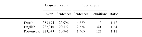
Table 1 displays a quantitative description of these corpora in terms of their original size (tokens and sentences), dataset size, number of positive examples (actual definitions marked by the human annotators) and the ratio between positive and negative examples.
Corpora description

The Dutch corpus is composed of 26 tutorials with a total size of 353,174 tokens and 23,996 sentences, of which 113 contain copula definitions. The corpus was annotated with morphosyntactic features with the Wotan tagger and with lemmas provided by the Corpus Gesproken Nederlands (CGN) lemmatizer (Westerhout and Monachesi, Reference Westerhout and Monachesi2007).
The English corpus is a collection of 7 tutorials with a total size of 287,910 tokens and 20,172 sentences, of which 40 contain copula definitions. The corpus is annotated with linguistic information, using the Stanford POS tagger (Toutanova and Manning, Reference Toutanova and Manning2000).
The Portuguese corpus contains 23 tutorials and scientific papers in the field of information technology and has a size of 223,049 tokens and 10,941 sentences, of which 121 contain copula definitions. It is automatically annotated with the LX-Suite (Branco and Silva, Reference Branco and Silva2006).
In order to prepare the dataset to be used in our experiments, all the sentences where the verb ‘to be’ appears as the main verb were extracted. For Portuguese, we obtained a sub-corpus composed of 1,360 sentences, 121 of which are definitions, with a ratio of about 1 to 11. For Dutch, we obtained a sub-corpus composed of 4,829 sentences, 120 of which are definitions, with a ratio of 1 to 42. Finally, for English, the sub-corpus is composed of 2,574 sentences, 40 of which are copula definitions, with a ratio of 1 to 64. These sub-corpora are datasets that were used to train and test the classifiers in the experiments reported below.Footnote 4
4.2 Feature selection
The selection of features was determined by the goal of enhancing the transportability of the solutions for definition extraction, that is, we wanted the type of features used to be, as much as possible, domain and language independent.
Looking at related work, commonly used features are bag-of-word, n-grams (Miliaraki and Androutsopoulos, Reference Miliaraki and Androutsopoulos2004) (either of POS or of base forms), the position of the definition inside the document (Joho and Sanderson, Reference Joho and Sanderson2000), or the presence of determiners in the definiens and the definiendum. Other relevant, more complex properties can be the presence of named entities (Fahmi and Bouma, Reference Fahmi, Bouma, Basili and Moschitti2006) or data from an external source such as encyclopedic data and WordNet (Saggion, Reference Saggion2004).
Some of these features may work well with a given corpus but not so well with another. The use of the position of a definition-bearing sentence in its document is an example of a feature that is corpus dependent. For instance, in encyclopedic documents, definitions appear at the beginning of documents, but the same did not happen in tutorials in our corpora.
In order to avoid such limitations, we represented instances as n-grams of POS. Currently, a POS tagger is a basic resource available for many natural languages.
After some preliminary experiments, the best choice turned out to be the adoption of bigrams. From each corpora, we extracted all the bigrams and then reduced the respective huge list using the information gain attribute evaluation algorithm (Witten and Frank, Reference Witten and Frank2005), thus obtaining a list of 50 bigrams for each dataset.
4.3 Sampling algorithms
In our evaluation, we selected a set of state-of-the-art sampling algorithms that are frequently used and referred to in the literature as delivering a good performance. We choose random (under and over) sampling algorithms as our starting point. We also selected the algorithms condensed nearest-neighbor rule, Tomek links, edited nearest neighbor, neighborhood cleaning rule as direct undersampling methods. In general, direct undersampling methods try to characterize each training example as borderline, noise or far from the decision border, and they discard a subset of the examples according to this classification. For instance, noise examples may be discarded as well as a subset of the examples far from the decision border, since those examples are usually less critical (or harmful) for learning.
Most of the direct undersampling algorithms were originally proposed as data cleaning methods. Therefore, they eliminate examples of both (minority and majority) classes. Unfortunately, for most imbalanced class datasets, the number of minority class examples is severely small, and discarding part of those examples would often make the learning impracticable. Therefore, these data cleaning algorithms were adapted as undersampling methods by simply retaining all minority class examples and applying the selection and filtering out over only the majority class examples.
We also use SMOTE as a direct oversampling algorithm. SMOTE creates synthetic minority class examples instead of replicating exact copies of these examples.
A short description of each algorithm is presented below:
Random oversampling consists of random replication of minority class examples, while in random undersampling, majority class examples are randomly discarded until the desired amount is reached. These two straightforward methods are often criticized. Several authors have pointed out that undersampling can potentially discard useful data that could be important for the induction process. In contrast, random oversampling can increase the likelihood of overfitting, since it makes exact copies of the minority class examples (Batista, Prati and Monard, Reference Batista, Prati, Monard, Famili, Kok, Peña, Siebes and Feelders2005).
Condensed nearest-neighbor rule (CNN) (Hart, Reference Hart1968) is a data cleaning method that finds a consistent subset in order to eliminate examples that are distant from the decision border, since these examples might be considered less relevant for learning. A subset E′⊂E is consistent with E if using 1-nearest neighbor, E′ correctly classifies the examples in E. An algorithm to find a consistent subset is: first, it randomly draws one example of each class from E and puts these examples in E′. Next, it uses a 1-NN algorithm over the examples in E′ to classify each example in E. Every misclassified example from E is moved to E′. We converted this method to an undersampling algorithm by adding to the subset generated by CNN all the minority examples it deleted. CNN is typically sensitive to noise, since noisy data are likely to be misclassified by its neighbors.
Tomek links (Tomek, Reference Tomek1976) algorithm is a data cleaning method that removes both noise and borderline examples. Tomek links are pairs of instances of different classes that have each other as their nearest neighbors. Given two examples Ei and Ej belonging to different classes, and d(Ei, Ej) the distance between Ei and Ej, a (Ei, Ej) pair is called a Tomek link if there is not an example Ek such that d(Ei, Ek)<d(Ei, Ej) or d(Ej, Ek)<d(Ei, Ej). If two examples form a Tomek link, then either of these examples is noise or both examples are borderline. As an undersampling method, only examples belonging to the majority class are eliminated. The major drawback of Tomek links is that this method can discard potentially useful data, since borderline examples are often important to characterize the decision border. This method has a higher order computational complexity and will run slower than the other algorithms.
Edited nearest-neighbor rule (ENN) (Wilson, Reference Wilson1972) is a data cleaning method, and it removes any example whose class label differs from the class of at least two of its three nearest neighbors. This algorithm was designed to identify and eliminate examples that are likely to be noise data, while retaining most of the data. Therefore, this method is not very effective to balance training data. As an undersampling method, we removed only majority class examples that disagree with their three nearest neighbors.
Neighborhood cleaning rule (NCL)(Laurikkala, Reference Laurikkala2001) is an undersampling method that uses a variant of Wilson's edited nearest-neighbor rule. NCL modifies the ENN in order to increase the data cleaning. For a two-class problem, the algorithm can be described in the following way: for each example Ei in the training set, its three nearest neighbors are found. If Ei belongs to the majority class and the classification given by its three nearest neighbors contradicts the original class of Ei, then Ei is removed. If Ei belongs to the minority class and its three nearest neighbors misclassify Ei, then the nearest neighbors that belong to the majority class are removed.
While these methods are direct undersampling techniques, SMOTE is an oversampling method that produces new synthetic minority class examples.
SMOTE (Chawla et al., Reference Chawla, Bowyer, Hall and Kegelmeyer2002) is an oversampling method that forms new minority class examples by interpolating between several minority class examples that lie together in the ‘feature space’. For each minority class example, this algorithm introduces synthetic examples along the line segments joining any/all of the k minority class nearest neighbors (in this work k is equal to 3). Synthetic samples are produced taking the difference between the feature vector (sample) under consideration and its nearest neighbors. The difference is multiplied by a random number between zero and one and added to the feature vector under consideration.
SMOTE, random over- and undersampling are methods designed to change class proportion, and can be implemented to provide any desired output class distribution, including balanced distribution. The remaining methods are adaptations of data cleaning approaches and consequently they typically do not guarantee any desired class distribution. We investigated if multiple passes of the methods Tomek links, ENN and NCL would reach a perfect balance between positive and negative examples. This result was obtained only with Tomek links. Even if we tried to force the other two to do so, they have a natural stop point, and depending on the nature of the size and the imbalance degree of the dataset, this stop point can occur before the balance is achieved.
All the described algorithms were first applied one by one and then coupled. In particular, we tried to pair undersampling algorithms with oversampling algorithms. Three different settings were tested: undersampling to 25, 50 and 75 per cent and subsequent oversampling. This way, it is possible to assess to which extent a given algorithm is more effective. Regarding ENN and NCL, when it was not possible to reach the desired class distribution (25, 50 or 75 per cent), we used the proportion returned by the undersampling algorithm and then applied the oversampling algorithm to achieve the balance point.
4.4 Classification algorithms
The selection of learning algorithms took into account two different considerations. First, the selection of algorithms that represent the state of the art for definition extraction and also for imbalanced data. Second, the possibility to cover different paradigms of algorithms for classification, having at least an algorithm representative of each learning paradigm. This way, different sampling techniques may be studied with respect to a larger range of classification algorithms. Six such algorithms were selected: naïve Bayes, C4.5, random forest, k-NN, SVM and voting feature intervals.
A brief description of these algorithms can be found below.
Naïve Bayes (John and Langley, Reference John and Langley1995) is a simple probabilistic classifier that is very popular in natural language applications. It is based on Bayes’ theorem, and its algorithm is known for assuming independence of features. In short, the independence means that the occurrence of a specific feature value is independent from the occurrence of any other feature value. In spite of its simplicity, it usually permits one to obtain results similar to the results obtained with more sophisticated algorithms. Two different implementations were evaluated: one in which the numeric estimator precision values are chosen using a kernel estimator for numeric attributes and another using a normal distribution. The latter obtained better overall performance, and for this reason only the results obtained with this configuration are presented.
C4.5 (Quinlan, Reference Quinlan1996) and random forest (Breiman, Reference Breiman2001) are two decision tree algorithms. The first is a relatively simple algorithm that splits the data into smaller subsets using the information gain in order to choose the attribute for splitting the data. The second is an ensemble consisting of a collection of decision trees. For each tree, a random sample of the dataset is selected (the remaining is used for error estimation) and for each node of the tree, the decision at that node is based on a restricted number of variables.
The k-NN algorithm (Aha, Kibler and Albert, Reference Aha, Kibler and Albert1991) is a type of instance-based learning, also called lazy learning because, unlike the algorithms above, the training phase of the algorithm consists only in storing the feature vectors and class labels of the training samples and all computation is deferred until the classification phase. In this phase, it computes the distance between the target sample and n samples in the dataset, assigning the most frequent class among the k nearest samples. As it is used by default in the literature, here we presented results for the learner generated also when k was set to 3.
The SVM algorithm tries to construct an N-dimensional hyperplane that optimally classifies data points as much as possible and separate the points of two classes as far as possible (Chang and Lin, Reference Chang and Lin2001). The goal of SVM modeling is to find the optimal hyperplane that separates clusters of vectors in such a way that cases with one category of the target variable are on one side of the plane and cases with the other category are on the other side of the plane. The vectors near the hyperplane are the support vectors.
The voted feature intervals (VFI) algorithm (Demiröz and Güvenir, Reference Demiröz and Güvenir1997) uses a scheme that calculates the occurrences of feature intervals per class, and classifies by voting on new examples using these intervals, which are constructed around each class for each attribute. This way, an example is represented by a set of feature intervals on each feature dimension separately. Each feature participates in the classification by distributing real-valued votes among classes. Higher weight is assigned to more confident intervals, where confidence is a function of entropy. The class receiving the highest vote is declared to be the predicted class.
All classifiers were built using the Weka workbench (Witten and Frank, Reference Witten and Frank2005). Regarding the evaluation, in order to use all the corpus data for training and testing, tenfold cross-validation was used.
5 Results
In this section, we report the experiments undertaken and their results. First, we describe the results obtained by running the classifiers trained with no previous sampling. Next, the results obtained by applying the sampling algorithms separately are described. Finally, we describe the results obtained when sampling algorithms are combined.
We assess our results using the well-known F-measure and AUC. The main purpose of reporting results in F-measure is to allow for comparison with other results previously published in the area. However, the comparison should be made with a word of caution, as previously discussed, since F-measure is influenced by the classes’ prior probabilities. AUC is the state-of-the-art measure for performance assessment of classifiers in the presence of class-imbalanced data.
In all the following tables, the results are displayed from left to right going from the least to the most imbalanced dataset. Hence, the results obtained with the Portuguese dataset (PT) appear first, then those with the datasets for Dutch (DU) and finally with the one for English (EN).
5.1 No sampling algorithms
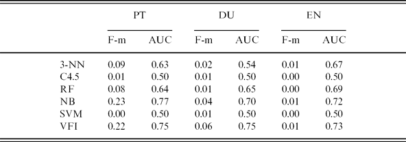
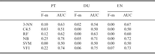
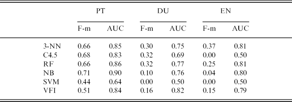
We start by showing, in Table 2, the performance results for learners when no sample algorithm is applied.
No sampling
They reveal that the performance of classifiers, in terms of F-measure, worsens when the class skewness increases, as we expected since this measure is influenced by the degree of imbalance. The same behavior is not so clear if we observe the AUC metric.
If we look at specific learners, the best performance in terms of AUC is obtained by naïve Bayes and VFI algorithms. In the literature on imbalanced datasets, it is assumed that a classifier should present an AUC of at least 0.75 to be considered reliable (Bradley, Reference Bradley1997). VFI achieves this value with the first two datasets, and it gets very close to it with the English dataset. Naïve Bayes only overcomes this threshold of 0.75 with the less imbalanced dataset, while for the other two it scores 0.70 and 0.72, respectively.
5.2 Single sampling algorithms
In this section, we present the experimental results obtained with a single pass of sampling algorithms. First, we present the results of random sampling, for balancing the training dataset so that it ends up with the same amount of negative and positive examples.
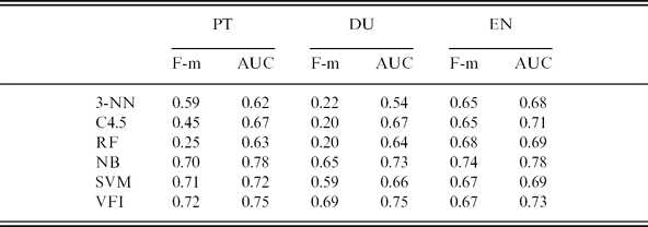
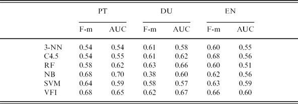
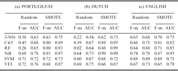
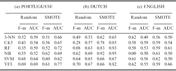
Tables 3 and 4, respectively, display the results for balanced datasets obtained with random oversampling and random undersampling. In both cases, the F-measure score highly improves with respect to no sampling. While with the original dataset the best result was of 0.23 for Portuguese, with both sampling algorithms, a value of around 0.70 is obtained for all the datasets. Regarding the AUC metric, it improves only with classifiers that obtained the worst performance when no sampling was used.
Random oversampling
Random undersampling
We now turn to the experiments with direct sampling techniques. From Tables 5 to 8, the results obtained with direct undersampling algorithms are presented.
Edited nearest neighbor (ENN)
Condensed nearest neighbor (CNN)
Neighborhood cleaning
Tomek links
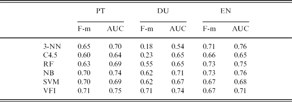
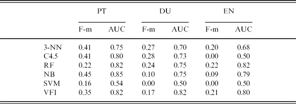
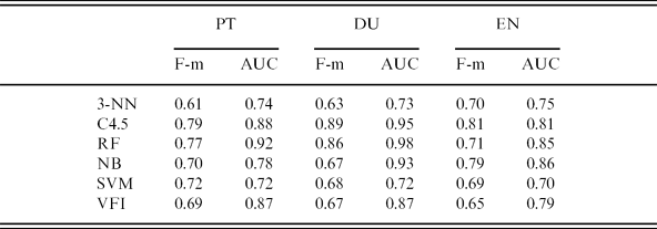
Turning our attention to these tables, it is possible to note the variation in performance when different undersampling algorithms are used. At one extreme, CNN (Table 6) obtains slightly worse results than those obtained with random undersampling. At the other extreme, Tomek links (Table 8) shows high performance in terms of both F-measure and AUC.
In the case of ENN (Table 5), the number of majority class items deleted was not enough to notably modify the degree of imbalance, so that the proportion of negative and positive examples remains the same as the original dataset, with no sampling. As mentioned in Section 4.3, this algorithm was developed for cleaning data, and even if it is applied recursively to the original dataset, eventually it will reach a stop point where no more examples can be deleted. As a consequence, the results are very similar to those obtained when no sampling algorithm is applied. We can conclude that for this kind of task (definition learning), in the way we have set the problem, this algorithm is not useful at all, at least when used alone.
CNN presents a different behavior (Table 6). In terms of F-measure, it presents higher scores than those for the original dataset (i.e. no sampling) and quite similar to those of random sampling. In terms of AUC, the scores worsen. In particular, this deterioration is more evident with classifiers that are getting better results with the original dataset. For example, looking at the Portuguese experiment, we can see that the VFI obtained a score of 0.75 (Table 2) with the original dataset and with CNN, it got 0.65. SVM obtained a score of 0.50 with the original dataset, while CNN now gets 0.59.
NCL shows a significant improvement compared to random undersampling (Table 7). Like ENN, this algorithm was not able to balance the dataset, but unlike ENN, it was able to modify the degree of imbalance. For each dataset, the following proportions were obtained: 1 to 3 for Portuguese (instead of 1 to 11), 1 to 17 for Dutch (instead of 1 to 42) and 1 to 28 for English (instead of 1 to 64). Since NCL did not achieve balanced datasets, it could be unfair to compare its results with the ones obtained with Tomek links. For this reason, a second experiment was run, setting Tomek links to reproduce the same proportion obtained by NCL for each dataset.
Table 9 shows the results of this experiment. In general, even when forced to reproduce the same data ratio returned by NCL, Tomek links outperforms NCL, with some differences among the datasets. The advantage of Tomek links is more evident with a less imbalanced dataset. As the imbalance increases, the two algorithms perform very similarly.
Not balanced Tomek links
It is also interesting to compare these results obtained by non-balanced Tomek links in Table 9 with those obtained by the same algorithm, only forced to return a perfectly balanced dataset (Table 8). In general, the balanced dataset obtains better results in terms of both F-measure and AUC, but the improvement is higher for the first metric. The only exception is the 3-NN based classifier. In this case, for all three datasets, the AUC value is higher when a non-perfectly balanced dataset is used.
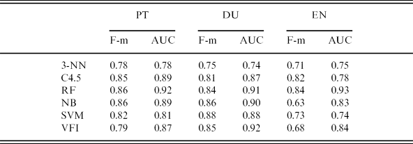
Given these considerations, Tomek links results to be the best undersampling algorithm for the definition extraction task. In terms of the AUC metric, only in two cases, this algorithm did not reach the threshold of 0.75, namely with 3-NN when using the Dutch dataset and with SVM when using the English dataset. However, in both cases the AUC value is 0.74, very near to the threshold. The best classifier, random forest, outperforms all other classification algorithms for all datasets, with AUC scores above 0.90. VFI and naïve Bayes algorithms follow at a short distance.
Regarding oversampling, when SMOTE (Table 10) is applied, results are very similar to those obtained with Tomek links, but with a slight difference. The threshold of 0.75 for AUC is not reached in five settings, namely for all datasets when SVM is used, and for Portuguese and Dutch datasets with 3-NN-based classifiers. When looking at specific classifiers, random forest maintains its advantage, but this time it is followed by C4.5 and then by VFI and naïve Bayes.
SMOTE
Finally, it is interesting to note that for less imbalanced datasets, Tomek links outperforms SMOTE. When the datasets are more imbalanced, the two algorithms deliver similar performances.
5.3 Combining sampling algorithms
In this section, we present and discuss the results obtained by combining under- and oversampling algorithms.
We opted for not reporting the results of the experiments carried out when oversampling is applied first. This is so because, as the number of examples increases, some algorithms are computationally very expensive, but above all because the performance was slightly worse than that obtained by doing undersampling first.
Each experiment is repeated for undersampling the majority class items to 75, 50 and 25 per cent of its initial size.
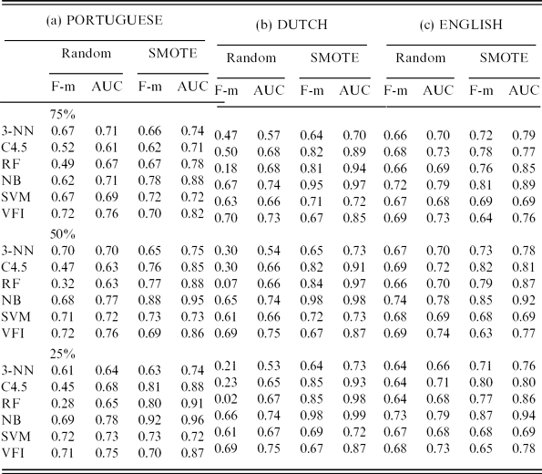
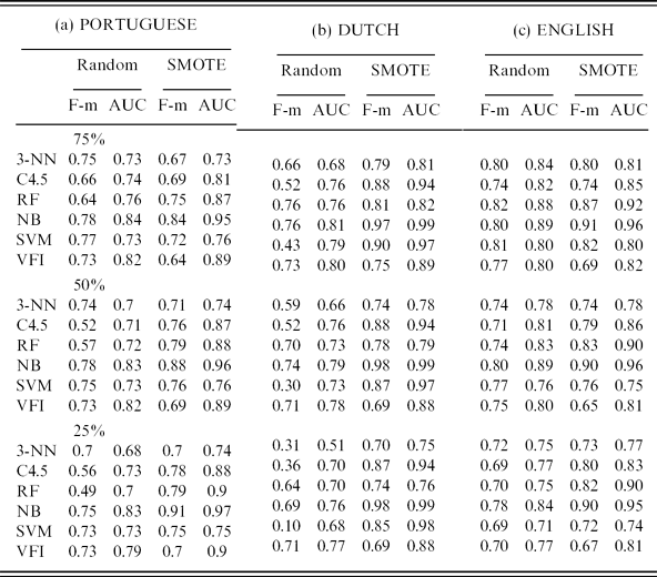
In the first experiment, we combined random undersampling with a random oversampling algorithm first and then with SMOTE. Table 11 shows the performance of classifiers for these two combinations.
Random undersampling plus oversampling (random and SMOTE)
When combining the two random algorithms, the performance does not improve, and the scores are quite similar to those obtained using just one such sampling algorithm.
Something similar happens when random undersampling is followed by SMOTE. Here, the results obtained are about the same as those obtained by SMOTE alone.
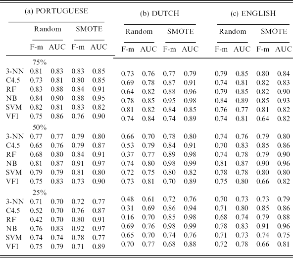
A different scenario can be observed when we turn to Table 12, which displays the results obtained by using Tomek links as the first algorithm in the sequence of sampling algorithms.
Tomek links plus oversampling algorithms
As for the combination of Tomek links with random oversampling, only when the majority class items are reduced to 75 per cent, results are better or similar to those obtained using Tomek links alone.
As for the combination of Tomek links with SMOTE, the situation is more complex. For 3-NN, SVM and VFI classifiers, the best results are obtained when Tomek links reduces the dataset to 75 per cent. Random forest and VFI work better when the reduction is 50 per cent. And, finally, C4.5 achieves the best performance with the third setting, with the maximum reduction of imbalance, down to 25 per cent.
It is interesting to note that in the case of the Portuguese dataset, the least imbalanced one, the improvement for most classifiers is not very significant, except when naïve Bayes is used. But as the skewness increases, the combination of the two algorithms generates better results in terms of F-measure and AUC for almost all classifiers when comparing the results obtained with either Tomek or SMOTE alone. For the Dutch and English datasets, this improvement occurs not only with the best setting but also with all three reduction levels considered.
Finally, it is worth noting that, for all classifiers in all datasets, the threshold of 0.75 is achieved.
When we turn to NCL, in Table 13, a similar scenario is observed. As the imbalance increases, the best results are obtained with the combination of the two sampling algorithms. In this case, for the Dutch and English datasets, the best performance is obtained when NCL reduces the initial datasets to 75 per cent of their size. For English, with this specific setting, all results are better than when SMOTE is used alone. On the contrary, for the Portuguese and Dutch datasets, it is possible to note that AUC gets worse with 3-NN, C4.5 and RF classifiers and improves with the other three.
Neighborhood cleaning rule (NCL) plus oversampling algorithms
Given the specificity of the remaining two undersampling algorithms, ENN and CNN (see Section 4.3), it is not possible to execute the three variants (75, 50 and 25 per cent) of each experiment.
The combination of ENN with oversampling, whose results are displayed in Table 14, permits us to achieve some improvement. By comparing these results with those in Table 10, for SMOTE alone, we observe that there is a small improvement for most classifiers when the combination of the two algorithms is used.
ENN rule plus oversampling algorithms
Finally, Table 15 displays the results for the undersampling with CNN. For the first time, it is possible to find results improving with some datasets but not with others.
CNN rule plus oversampling algorithms
In this experiment, for the Dutch dataset, the results obtained in terms of F-measure are comparable to those obtained with SMOTE alone. As for the AUC scores, these are just slightly worse than those obtained with SMOTE alone.
With the Portuguese and English datasets, in turn, results are worse than those obtained with either CNN alone or with SMOTE alone.
To understand these results, it is important to note that, for different datasets, CNN returns different proportions between the positive and negative classes. In particular, in this experience, it delivered 1:2 for the Portuguese dataset, 1:7 for the Dutch dataset, and 1:1.5 for the English dataset. Given the lowest ratio obtained for the Dutch dataset, this implied that the larger portion of the balancing work was left to the SMOTE algorithm, and this explains why the final results were better in this case.
6 Discussion
From the systematic experimentation carried out with respect to the task of definition extraction reported above, a number of lessons can be gathered.
Sampling imbalanced datasets frequently improves the performance of classifiers over the baseline, which is in the range of 0.73–0.77 in terms of the AUC score.
However, not all sampling techniques are equally suited to foster this improvement. Some of them add very little improvement, if any. That is the case of random over- and undersampling and ENN. Some others may even deteriorate the results to deliver scores clearly below the baseline. That is the case of CNN.
For undersampling, NCL and Tomek links consistently helped to improve the performance of classifiers, as well as SMOTE, for oversampling, with AUC results in the range of 0.82–0.98. Tomek links should be pointed out as one of the best options as it exhibits an equal top performance for datasets with different imbalance degrees, with AUC in the range of 0.92–0.93.
In general, combining undersampling with oversampling provides better results than when only one of them is used. Better results were obtained performing undersampling before oversampling, and using direct oversampling with SMOTE instead of just plain random oversampling. The exception is found again when CNN is chosen as an undersampling method. But all other combinations (including those with random undersampling as the first step) have consistently shown to be able to raise the AUC scores to the range of 0.94–0.99.
The best performing combinations are the ones that result from combining the algorithms that had been shown to be the best in their categories when applied in isolation. That is, the best results are obtained with NCL or Tomek links for undersampling and SMOTE for oversampling.
Which sampling method should be preferred will largely depend on the computational cost associated with the use of these two algorithms. In fact, as mentioned above, the use of oversampling algorithms increases the computational cost because it increases the number of examples that will be used to build the classifier. In contrast, Tomek links is a very complex algorithm that, for every example, considers all examples in order to identify a link. This means that the time needed to undersample the dataset is polynomially related to the size of the original dataset. Due to the growth in computational capacity of computers, it is likely that this question may not represent a real issue for many applications.
In general, there seems to exist a tendency for the largest extension of the undersampling to permit the best results, and hence for less catch-up work to be required for the oversampling step. When undersampling to just 75 per cent, the scores are in the range of 0.93–0.99, while they are in the range of 0.96–0.99 for undersampling to as much as 25 per cent. But more firm conclusions on this respect would perhaps need to be based on datasets with a larger range of number of tokens.
Interestingly, the best results – that is, when undersampling and oversampling are combined – are consistently obtained by the naïve Bayes classifier. Also consistently, the second best option is the random forest classifiers, though at a clear distance behind.
It is interesting to note that these two classifiers are among the best ones even when no sampling algorithms are used. This result suggests that, for the learning algorithms used in this work, naïve Bayes and random forest have the most suited learning bias for the task of definition extraction. Therefore, the sampling algorithms are responsible for just leveraging off the classification performance of these algorithms, given the imbalanced characteristic of the data. The reason of why the learning bias of these algorithms is suited for definition extraction is out of the scope of this work. However, we note that it is in conformity with theoretical and practical results present in the literature. For instance, naïve Bayes frequently presents good performance in natural language processing (Roth, Reference Roth1999) even when the model assumptions of independence do not hold (Zhang, Reference Zhang2005). Regarding random forest, ensemble classifiers are one of the most effective computationally intensive procedures to improve on unstable estimators or classifiers, being useful especially for high-dimensional dataset problems (Biau, Reference Biau2012).
The same tendencies can be observed with F-measure scores. The best combinations of undersampling, oversampling and classifier algorithms consistently deliver performances scoring in the range of 0.87–0.99 in terms of F-measure.
Looking more closely at the scores obtained by naïve Bayes and random forest, there is a difference in terms of precision and recall. For all the three languages, random forest classifiers were able to obtain a recall close to one, that is all the definitions were correctly identified, but there is a larger number of non-definitions classified as positive examples in comparison to what happens with naïve Bayes classifiers.
In order to generalize our results, we tested our approach with definitions introduced by verbs other than ‘to be’, such as ‘to mean’, ‘to signify’ etc. When all these kinds of verbs are considered together, the degree of imbalance is slightly smaller than the imbalance in the definitions introduced by the verb ‘to be’ alone. Preliminary results present an F-measure around 0.78 and an AUC around 0.83, confirming the combination of Tomek links and SMOTE as the best sampling method and naïve Bayes as the best learning algorithm. In this experiment, the same classifier identified definitions introduced by different verbs, while in the previous experiments there was a classifier specialized just on the definitions introduced by the verb ‘to be’. If a classifier for each different verb or a classifier for a group of similar verbs were used, results similar to those obtained for ‘to be’ definitions are expected.
When comparing with previous work on definition extraction, our results outperform all the systems that have used learning algorithms, confirming the importance of sampling techniques in supporting the definition extraction task.
Westerhout and Monachesi Reference Westerhout and Monachesi2007, using the same corpus we used for Dutch, report an F-measure of 0.73, obtained with a combination of syntactic rules and a naïve Bayes classifier for Dutch. Przepiórkowski, Marcińczuk and Degórski Reference Przepiórkowski, Marcińczuk and Degórski2008, in turn, with a similar approach, but for the Polish language, obtained an F-measure of 0.35. Additionally, it is very important to note that, while our experiments just use bigrams of POS tags as features, all these previous works use a combination of sophisticated and highly language dependent features in order to reach the best results.
As in the last few years, balanced random forest has been successfully used in different classification tasks (see for instance Acedański et al. Reference Acedański, Slaski and Przepiórkowski2012) and in order to try a more direct comparison between our results and those obtained by Degórski et al. Reference Degórski, Kobyliński and Przepiórkowski2008a and Westerhout Reference Westerhout2009, we run this algorithm on our datasets. In this way, we obtained an F-measure of 0.73, 0.58 and 0.48 for Portuguese, Dutch and English, respectively. With respect to results obtained with different sampling techniques presented here, these scores are comparable to those returned by random sampling. With respect to Westerhout Reference Westerhout2009, where the same Dutch dataset was used, resulting in an F-measure of 0.78, a direct comparison is not possible, since balanced random forest was used as a filtering module after the application of a quite elaborate pattern module, and also because more sophisticated features were used. In the case of Degórski et al. Reference Degórski, Kobyliński and Przepiórkowski2008a, which reports an F-measure of 0.32, a different dataset and feature selection were used, making direct comparison not viable.
If we now turn to systems based only on pattern matching ensured by hand-crafted rules, the state of the art in the area is represented by systems such as DEFINDER (Klavans and Muresan, Reference Klavans and Muresan2001), which is reported to have an F-measure of 0.80. Though not strictly comparable due to the use of different experimental conditions, including different datasets for evaluation, our approach seems to deliver results above this performance by a large margin, with scores in the range of 0.90–0.99.
Also when put into contrast with the usage of this same approach to other natural language processing tasks, our results seem to be very competitive. As discussed in Section 2.3, Liu et al. Reference Liu, Chawla, Harper, Shriberg and Stolcke2006 applied a combination of under- and oversampling to sentence boundary detection in speech, showing that undersampling and SMOTE offer the best results with an AUC of 0.89 (the baseline being 0.80). However, they did not experiment intelligent undersampling methods such as Tomek links.
In another task, of automated annotation of keywords, Batista, Bazzan and Monard Reference Batista, Bazzan, Monard, Lifschitz, Almeida, Pappas and Linden2003 get the best results in terms of AUC with an improvement of four percentage points on the original dataset using a combination of SMOTE with Tomek links.
In our case, with scores in the range of 0.94–0.99, the improvement with regard to the baseline of 0.73–0.77 is at least between 17 and 22 percentage points, demonstrating how these methods can be effective for our definition extraction application.
Finally, it is worth noting that our results are in line with those reported in the literature on imbalanced datasets in general. In a comprehensive study on the behavior of several methods for balancing training data, using 11 UCI datasets,Footnote 5 Batista, Prati and Monard Reference Batista, Prati and Monard2004 showed that in most cases and with several datasets in different domains, SMOTE obtains the best performance. In general, they lead to a rise in the AUC metric of few percentage points (1–4) when the baseline was already high (more than 0.65), while when the baseline was under this value the improvement was comparable to that obtained in our work, which was up to 34 percentage points.
We also conducted a qualitative analysis on the examples not correctly classified by our approach. In particular, we analyzed the results of the best settings, that is when Tomek links is paired with SMOTE and naïve Bayes and random forest are used as classification algorithms. As for all the three languages, the random forest classifier was able to obtain a recall of one, we do not have false negatives to analyze.
Regarding false-positive examples, that is, those sentences that were incorrectly classified as definitions, in few cases we verified that they were good definitions but the human annotators had just missed them. In about one-fifth of the cases, sentences contained some definitional information, but the human annotators did not annotated these sentences as definitions because the definition spanned over several sentences. For instance, there are several cases where the defined term appears in a sentence, and its definition in the following sentence.
There is another set of sentences starting with demonstrative pronouns that are considered by the classifier as good definitions though they are not. Most of these sentences are referring to illustrations in the text. In this case, the results could be filtered either by improving the features that include information appearing before the definitional verb or with a simple grammar to be applied after or before the classifier.
In terms of false-positive examples, there is no big difference between naïve Bayes and random forest classifiers. Regarding false-negative examples, they appear only in naïve Bayes classifiers. They occur mostly when the definition is composed of only the genus or the diferentiae.
7 Conclusions
The advances reported in the present paper result from a novel approach to the task of definition extraction. The major trend in the literature has been to build solutions for this task on the basis of some set of manually crafted patterns. In the present paper, we experimented thoroughly with an alternative solution based solely on machine learning techniques. The key twist to make such an approach not only viable but also with superior results was to focus on the issue of the imbalance of datasets. This permitted us to take advantage of the solutions that have been put forward to this problem in recent years, and eventually find out that they allow for a notable breakthrough in terms of the task of definition extraction.
The results obtained with our experiments show that it is feasible to consistently bring the performance of an automatic extractor of definitions to score in the range of 0.95–0.99 in terms of AUC (and in the range of 0.90–0.99 in terms of F-measure). The improvement with regard to the baseline of 0.73–0.77 is thus at least between 17 and 22 percentage points.
Very interestingly, these advances were obtained not only by dispensing with manually crafted patterns but also by resorting only to bigrams of POS tags (as features for the classifiers), thus greatly improving the transportability of the approach both across domains and languages.
On par with these overall advances, by systematically experimenting with different paradigms of learning algorithms in combination with different sampling techniques, and with datasets with different imbalance rates, it was possible to draw some finer conclusions regarding the best practice to adopt when handling automatic definition extraction.
In particular, the most effective set-up has shown to be a combination of Tomek links, for undersampling, followed by SMOTE, for oversampling, even more so when datasets with higher imbalances have to be dealt with.
As for the set-up with only one step of dataset imbalance reduction, we can conclude that Tomek links is the best choice. This algorithm improves the result for all classifiers and for all datasets, independent of the degree of their imbalance or of their language, while SMOTE tends to be less effective with higher data skewness.
As for the classifiers used for this task of definition extraction, random forest and naïve Bayes present the best results in almost all the experiments, with a significant difference between the two classifiers in terms of recall and precision: naïve Bayes performs better in terms of precision, while random forest gets a higher score for recall.
We can thus observe that, under this approach, the best way to construct a definition extractor is to build a naïve Bayes classifier after sampling the dataset using a combination of Tomek links followed by SMOTE.
As a final remark, it is worth noting that the present results not only represent a progress in the area of automatic extraction of definitions, but they also reinforce the value of using sampling techniques in the field of natural language engineering, where most tasks and tools rely on datasets with notorious imbalance. The present paper adds to the seminal work that point toward the important research avenue of seriously applying sampling techniques to mitigate the adverse bias induced by highly imbalanced datasets and thus greatly improving the performance of a range of tools for natural language processing.