

Introduction
Conservation paleobiology is a rapidly developing field that aims to integrate paleontological data and approaches with the practice of conservation biology in order to mitigate anthropogenic impacts on ecosystems (Dietl and Flessa Reference Dietl and Flessa2011, Reference Dietl and Flessa2017; Dietl et al. Reference Dietl, Kidwell, Brenner, Burney, Flessa, Jackson and Koch2015; Kidwell Reference Kidwell2015; Dietl Reference Dietl2016; Barnosky et al. Reference Barnosky, Hadly, Gonzalez, Head, Polly, Lawing, Eronen, Ackerly, Alex, Biber, Blois, Brashares, Ceballos, Davis, Dietl, Dirzo, Doremus, Fortelius, Greene, Hellmann, Hickler, Jackson, Kemp, Koch, Kremen, Lindsey, Looy, Marshall, Mendenhall, Mulch, Mychajliw, Nowak, Ramakrishnan, Schnitzler, Das Shrestha, Solari, Stegner, Stegner, Stenseth, Wake and Zhang2017). Much conservation paleobiology work hinges on the assumption that death assemblages—nonliving material accumulated from a living assemblage in near time (Boucot Reference Boucot1953; Kidwell and Bosence Reference Kidwell and Bosence1991)—have reasonably good fidelity with living assemblages, or at least that processes that alter death assemblages from the original living assemblages can be understood and quantified (e.g., Kidwell Reference Kidwell2013; Kidwell and Tomašových Reference Kidwell and Tomašových2013; Dietl et al. Reference Dietl, Kidwell, Brenner, Burney, Flessa, Jackson and Koch2015). Generally, living assemblages and death assemblages have similar taxonomic composition and rank order, whereas proportional abundance in death assemblages shows somewhat less fidelity to living assemblages (Kidwell and Bosence Reference Kidwell and Bosence1991; Kidwell Reference Kidwell2001, Reference Kidwell2013; Kidwell and Tomašových Reference Kidwell and Tomašových2013). Areas with known anthropogenic impacts can exhibit mismatch between living and death assemblages, which conservation paleobiologists attribute to alteration of the living assemblage from some previous state (Kidwell Reference Kidwell2007, Reference Kidwell2013; Kidwell and Tomašových Reference Kidwell and Tomašových2013). However, biases attributable to the assemblage members themselves, rather than anthropogenic influence, could cause live–dead mismatch. For instance, differences in individual life spans may alter species rank order and proportional abundance, though this potential bias has not been studied widely.
The concept of a bias related to differential species life span is straightforward: short-lived species contribute multiple individuals to the death assemblage in the time it takes for species with longer maximum life spans to contribute a single individual (Van Valen Reference Van Valen1964). Life span differences thus lead to death assemblages in which short-lived species are overrepresented (proportional abundances rise) and long-lived species are underrepresented (proportional abundances fall) compared with their respective abundances in living assemblages. The degree of distortion between the proportional abundances in the living and death assemblages is expected to increase with increasing life span disparity among species (Van Valen Reference Van Valen1964).
Kidwell and Rothfus (Reference Kidwell and Rothfus2010) named this bias due to differential species longevity “life span bias” and quantified its effects on molluscan death assemblages in shallow-marine settings. Bivalve mortality rates were calculated from maximum life spans gleaned from the literature and used to predict proportional abundances of species in death assemblages (Kidwell and Rothfus Reference Kidwell and Rothfus2010). Expected dead proportional abundances were compared with the proportional abundances observed in the death assemblages to assess the ability of a species’ life span to predict live–dead discordance (Kidwell and Rothfus Reference Kidwell and Rothfus2010). Only ~10% of discordance between the live and dead proportional abundances of species across 30 live–dead studies could be accounted for by life span differences, a result that was described as contributing “low level noise” relative to the other factors influencing live–dead discordance (Kidwell and Rothfus Reference Kidwell and Rothfus2010: p. 616).
However, life span better predicted live–dead discordance among two groups (Kidwell and Rothfus Reference Kidwell and Rothfus2010). First, species with life spans longer than the median (9 years) for bivalves in the database better fit the expectations of the life span bias model and were therefore termed “‘well behaved’ long-lived species” (Kidwell and Rothfus Reference Kidwell and Rothfus2010: p. 627). The coefficient of determination for correlations of predicted live–dead discordance and observed discordance was higher for long-lived species (r 2=0.24 to 0.31) than for short-lived species (r 2 ≈ 0), which may be attributed to greater long-term stability in live standing abundance (Kidwell and Rothfus Reference Kidwell and Rothfus2010). Second, life span bias better predicted observed discordance for species with known life spans than for species with estimated life spans (Spearman rho2=0.15 vs. 0.03; Kidwell and Rothfus Reference Kidwell and Rothfus2010). Maximum ages were known for only 32% of the species occurrences; the remaining two-thirds were estimated from median life spans of congeners, confamilial genera, or from all bivalves in their data set (Kidwell and Rothfus Reference Kidwell and Rothfus2010). Because life spans can vary widely within both families and genera (e.g., Veneridae: 1–106 years, Mytilidae: 1–150 years, Anadara 2.5–30 years, Glycymeris: 20–192 years; Moss et al. Reference Moss, Ivany, Judd, Cummings, Bearden, Kim, Artruc and Driscoll2016: Supplemental Data), life spans derived from related species could significantly over- or underestimate species-specific maximum life spans. Maximum life spans of individuals can also vary substantially for species with large geographic ranges (Moss et al. Reference Moss, Ivany, Judd, Cummings, Bearden, Kim, Artruc and Driscoll2016: Supplemental Data). Phylogenetic and geographic interpolations of life span across individuals within species remains an untested factor in the attribution of live–dead discordance to life span bias.
Kidwell and Rothfus (Reference Kidwell and Rothfus2010) suggested that local life span data could improve predictions of live–dead discordance, but neither of the two studies that have since considered the effects of life span bias on live–dead discordance included local life spans (Albano and Sabelli Reference Albano and Sabelli2011; Martinelli et al. Reference Martinelli, Madin and Kosnik2016). We suspect the paucity of studies is due in part to the labor-intensive nature of determining the maximum age for all species in an assemblage. Here, we directly determined the ontogenetic ages of individuals of two long-lived bivalve species—Mercenaria mercenaria (Linnaeus, Reference Linnaeus1758) and Chione elevata (Say, Reference Say1834)—and analyzed life span bias using calculation methods adapted from Kidwell and Rothfus (Reference Kidwell and Rothfus2010) to compare only two species rather than entire assemblages. Additionally, local and regional life spans were compared with global life spans to assess their ability to predict discordance between proportional abundance in living and death assemblages.
This study tested three separate but related hypotheses:
1. The ratio of live-collected C. elevata to M. mercenaria will differ from their corresponding ratio in the death assemblage, with the shorter-lived C. elevata overrepresented in the death assemblage compared with its live proportional abundance.
2. The magnitude of the difference in ratios can be predicted by the magnitude of the difference in mortality rates calculated from the life spans of C. elevata and M. mercenaria.
3. The life span bias calculated using local life span values will predict the magnitude of the shift in ratios better than life span bias calculated from global maximum life spans.
Materials and Methods
Study Organisms
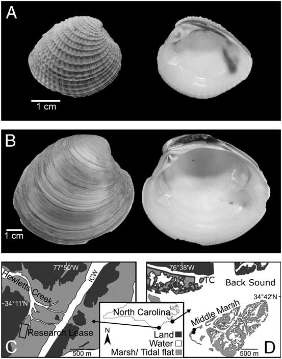
Chione elevata (Fig. 1A) and M. mercenaria (Fig. 1B) are common co-occurring venerid bivalves in the southeastern United States. Both species are shallow-burrowing filter feeders with similar sets of natural predators and relatively thick, durable shells—similarities that minimize the potential for preservation biases to confound any bias due to their differential life spans. Additionally, because maximum life spans for both species exceed 9 years, they are also likely to be “‘well behaved’ long-lived species” with life span bias explaining more of the observed discordance between living and death assemblages (Kidwell and Rothfus Reference Kidwell and Rothfus2010: p. 627).
Study organisms and sites. A, Exterior and interior view of Chione elevata right valve. Individual was 2 years old, collected from Research Lease. B, Exterior and interior view of Mercenaria mercenaria right valve. Individual was 4 years old, collected from Research Lease. C, Research Lease at the University of North Carolina Wilmington, near the mouth of Hewletts Creek. Individuals were collected from mudflats within the black rectangle. ICW, Intracoastal Waterway. D, Middle Marsh in Back Sound near the mouth of Taylor Creek (TC), Beaufort, North Carolina. Individuals were collected from the seagrass beds indicated on the map by the black dots.

The two species have distinct average life spans; M. mercenaria lives an average of 25 years under natural conditions (Loesch and Haven Reference Loesch and Haven1973), whereas Edie and Surge (Reference Edie and Surge2013) found that the majority of C. elevata were between 2 and 3 years old. Maximum life spans for each species are also documented and disparate: the global maximum age is 106 for M. mercenaria (Ridgway et al. Reference Ridgway, Richardson, Enos, Ungvari, Austad, Philipp and Csiszar2011) and 11 for C. elevata (Edie and Surge Reference Edie and Surge2013). Ages for individuals of both species can be determined accurately without isotope analysis at our study sites (Peterson et al. Reference Peterson, Duncan, Summerson and Beal1985; Jones et al. Reference Jones, Quitmyer, Arnold and Marelli1990; Edie and Surge Reference Edie and Surge2013), allowing us to determine not only a maximum life span based on individuals collected at each site, but also a detailed age-frequency distribution (AFD) for each species at each site from which to calculate an alternative local mortality rate.
Field Sites and Sampling Protocol
Live and dead M. mercenaria and C. elevata were sampled from two sites in North Carolina: the University of North Carolina Wilmington Research Lease (hereafter Research Lease) located at the mouth of Hewletts Creek near Masonboro Inlet (Fig. 1C; 34.175604°N, 77.841901°W), and Middle Marsh in Back Sound near Beaufort (Fig. 1D; 34.694316°N, 76.610095°W). Both sites are intertidal, and sediment consists of mixed mud and sand. Seagrass beds were targeted for sampling at Middle Marsh, because they contain higher densities of both M. mercenaria and C. elevata than mudflats or sand flats (Peterson Reference Peterson1982; Peterson et al. Reference Peterson, Summerson and Duncan1984). The Research Lease samples were collected from the mudflat; seagrass beds were absent at this site.
Sixteen ~2 L bulk samples were collected from the mudflat at Research Lease on 2 April 2010. In total, 50 bulk samples (each ~50 L) were collected at Middle Marsh from two seagrass beds; 31 samples from one bed were collected over 4 days in June 2014, February 2015, and March 2015, and 19 samples were collected from an adjacent seagrass bed in August 2015. At both Research Lease and Middle Marsh, samples were collected from within the first 20 cm below the sediment surface, representing the taphonomically active zone (Davies et al. Reference Davies, Powell and Stanton1989). Both species primarily remain near the sediment surface in life position, though C. elevata can burrow to 30 cm and M. mercenaria to 20 cm (Moore and Lopez Reference Moore and Lopez1969; Eversole Reference Eversole1987; Roberts et al. Reference Roberts, Rittschof, Gerhart, Schmidt and Hill1989). Samples were sieved in the field through 5-mm mesh to ensure that juveniles and postsettlement larvae were excluded from the samples, as they do not preserve well in death assemblages (Kidwell Reference Kidwell2001).
Establishing Observed Species Ratios and Life Span Determination
All live and dead M. mercenaria and C. elevata were removed from the sieved material. Live individuals were sacrificed. All whole dead valves and fragments that retained a hinge and umbo were assigned to right or left valve groups and counted. The ratio of right to left valves was used to evaluate whether one valve type experienced preferential transport. The number of individuals was based on the number of right valves in a sample; counts of right valves were converted to ratios of live C. elevata to live M. mercenaria and dead C. elevata to dead M. mercenaria, called observed live and observed dead (after observed live and observed dead proportional abundances; Kidwell and Rothfus Reference Kidwell and Rothfus2010). Ratios and ages of right valves were used in the calculations to assess life span bias (see “Life Span Bias Calculations” section).
Right live and dead valves were cleaned, dried, and ontogenetically aged. Chione elevata ages were determined by counting concentric exterior notches (CENs) on the surface of each right valve (after Edie and Surge Reference Edie and Surge2013). Additional growth after the final identifiable CEN was ignored, so the assigned age was equal to the number of CENs on the valve. Mercenaria mercenaria ages were determined by examining growth bands in cross section (after Peterson et al. Reference Peterson, Duncan, Summerson and Safrit1983). Right valves were sectioned with a diamond band saw along the axis of maximum growth from umbo to margin. Dark purple summer growth bands visible in cross section were counted, as they represent a reliable annual marker of M. mercenaria shell growth in North Carolina (Peterson et al. Reference Peterson, Duncan, Summerson and Beal1985). Additional growth of white shell after the final dark summer band was ignored, so the assigned age was equal to the number of dark purple bands on the valve.
AFDs were constructed from a subset of the right valves. Valves were included in the AFDs if the margin along the axis of maximum growth was present and preservation allowed age determination (C. elevata with visible CENs and M. mercenaria with bands visible in cross section). AFDs included only individuals aged ≥1 year. Chione elevata reach sexual maturity at ~1 year (Moore and Lopez Reference Moore and Lopez1969) and a shell height of typically 5–10 mm in our samples. Mercenaria mercenaria typically reproduce at 20–25 mm shell height (Eversole Reference Eversole2001), which corresponded to individuals older than 1 year in our samples. Valves that were too worn or degraded for age determination, fragmented with incomplete margins, or <1 year in age were excluded from the AFDs but were counted in the observed live and observed dead ratios.
Life Span Bias and Live–Dead Discordance
We adapted the life span bias calculations and terminology used by Kidwell and Rothfus (Reference Kidwell and Rothfus2010) for whole-assemblage data to analyze only two species. We also calculated additional mortality rates based on regional and local maximum ages and AFDs to compare their ability to predict discordance with that of global maximum ages. In short, a theoretical death assemblage ratio, the expected dead ratio of C. elevata to M. mercenaria, was calculated using each species mortality rate and standing live abundance at each site. To establish life span bias (the difference expected between the observed live ratio and the theoretical expected dead ratio), the theoretical expected dead ratio was compared with two observed ratios, observed live and observed dead, and the amount of actual discordance between the observed live and observed dead ratios that could be explained by life span bias. Specific calculations are detailed below; an example calculation can be found in the Appendix.
Mortality Rate Calculations
Mortality rates were calculated using three maximum ages for each species: tmaxGlobal is the species-wide maximum age recorded in the literature, the metric used by Kidwell and Rothfus (Reference Kidwell and Rothfus2010); tmaxRegional is the regional (here defined as within North Carolina) maximum recorded age for each species; and tmaxLocal is the site-specific maximum age for each species from the oldest directly aged individual of each species found at each site. Mortality rates were also calculated from the AFDs of the directly aged individuals at each site. All calculations assume abundance, recruitment, and mortality rate remained constant over time; see Kidwell and Rothfus (Reference Kidwell and Rothfus2010) for a discussion of the implications of these assumptions.
The oldest known M. mercenaria was collected live at 106 years old (tmaxGlobal) near Cape Cod, Massachusetts (Ridgway et al. Reference Ridgway, Richardson, Enos, Ungvari, Austad, Philipp and Csiszar2011); the oldest known M. mercenaria from North Carolina was 46 years old (tmaxRegional) and was collected less than 25 km from the Middle Marsh site (Peterson et al. Reference Peterson, Summerson and Duncan1984). An 11-year-old specimen collected from Research Lease (Edie and Surge Reference Edie and Surge2013) is, to the best of our knowledge, the oldest recorded age for C. elevata before this study. This age was used for both regional (tmaxRegional) and global (tmaxGlobal) C. elevata maximum ages.
Following Kidwell and Rothus (2010), for all values of tmax, the instantaneous mortality rate (Z) was calculated using eq. (1) (Hoenig Reference Hoenig1983):
 $${\rm Ln}\left( Z \right){\equals}1.23{\plus}\left[ {{\minus}0.832{^\asterisk}{\rm ln}\left( {{\rm t}_{{{\rm max}}} } \right)} \right]$$
The constants −0.832 and 1.23 are the slope and y-intercept, respectively, of a linear regression of log mortality rate on log maximum age from 13 molluscan species from 28 unexploited to lightly exploited stocks (Hoenig Reference Hoenig1983). This calculation corresponds to step 1a in the Appendix. Also called the instantaneous mortality coefficient, Z is the slope of the portion of a species survivorship curve that describes adult survivorship. As species life span decreases, Z increases. A species with a 1-year life span has a Z of ~3.4, whereas a species that lives 100 years has a Z of ~0.07. Instantaneous mortality rate was converted to annualized mortality rate, via eq. (2):
 $${\rm Annualized}\,{\rm mortality}\,{\rm rate}{\equals}1{\hbox -}{\rm e}^{{{\minus}Z}} $$
This calculation corresponds to step 1b in the Appendix. Annualized mortality rates can range from 0 to 1; higher values indicate a shorter life span. For instance, the annualized mortality rate would be ~0.97 for a species with a 1-year life span and ~0.07 for a species with a life span of 100 years.
AFDs constructed for each site were also used to calculate Z using the Chapman-Robson method with corrections for bias and overdispersion in the variance (eq. 3; Seber Reference Seber1982; Smith et al. Reference Smith, Then, Wor, Ralph, Pollock and Hoenig2012).
 $$\eqalignno {{\rm CR}(\hat{Z}) {\equals}{\rm log}_{e} \left( {{{1{\rm }{\plus}{\rm }\bar{T}{\minus}T_{{\rm C}} {\minus}{1 \over N}} \over {{\rm }\bar{T}{\minus}T_{{\rm C}} }}} \right) \cr {\minus}{{(N{\minus}1)(N{\minus}2)} \over {N[N\left( {\bar{T}{\minus}T_{{\rm C}} } \right){\plus}1][N{\plus}N\left( {\bar{T}{\minus}T_{{\rm C}} } \right){\minus}1]}}$$
where T
C=age of full recruitment,
 $\bar{T}$
=mean age of individuals with ages ≥T
C, N=the number of individuals with ages ≥T
C.
The Smith et al. (Reference Smith, Then, Wor, Ralph, Pollock and Hoenig2012) method has the additional advantage of providing accurate Z values at sample sizes below 600, as was the case for M. mercenaria sampled from both Research Lease and Middle Marsh; however, the difference between Z calculated using the corrected method and Z calculated using the uncorrected Chapman-Robson method was never more than 0.01. Just as with Z calculated from the tmax values, Z values calculated from AFDs were then converted to an annualized mortality rate via eq. (2).
Life Span Bias Calculations
For each method of calculating mortality rate (tmaxGlobal, tmaxRegional, tmaxLocal, and AFDs), a pair of life span bias calculations were performed for each site to find the ratios of C. elevata to M. mercenaria expected in the death assemblages based on life span. First, the annualized mortality rate calculated for each species was multiplied by the standing live abundance of that species to determine the number of individuals of each species that should be contributed to the death assemblage each year, the expected numerical dead abundance (step 2a in the Appendix). Second, the expected numerical dead abundance for each species for each mortality rate value was converted to a ratio of C. elevata to M. mercenaria (step 2b in the Appendix). Assuming that mortality rate and standing live populations were constant over time, the ratio of C. elevata to M. mercenaria contributed to the death assemblage each year will equal the ratio of C. elevata to M. mercenaria in the entire death assemblage (Kidwell and Rothfus Reference Kidwell and Rothfus2010). This ratio was designated the “expected dead” here, as in the expected dead proportional abundances of Kidwell and Rothfus (Reference Kidwell and Rothfus2010).
Life span bias (LB), the expected discordance between the live and dead ratios based on each species mortality rate, was calculated as the difference between the expected dead ratio and the observed live ratio of C. elevata to M. mercenaria (calculated in step 3 in the Appendix; Kidwell and Rothfus Reference Kidwell and Rothfus2010). Negative LB values indicate that a species is expected to decrease in proportional abundance in the death assemblage, whereas positive LB values indicate a species is expected to increase in proportional abundance in the death assemblage. Observed discordance (OD) is the actual difference between live and dead ratios based on the counts of live and dead individuals at each site, calculated as the difference between the observed dead ratio and the observed live ratio (calculated in step 4 in the Appendix). As with LB, negative values of OD indicate a reduction in proportional abundance in the death assemblage, whereas positive OD values indicate an increase in proportional abundance in the death assemblage.
Kidwell and Rothfus’s (Reference Kidwell and Rothfus2010) method for assessing the amount of OD that can be explained by LB is inappropriate for an analysis with only two species; here, LB/OD expresses the amount of predicted life span bias that can be explained by the data (step 5 in the Appendix). Values of LB/OD>1 indicate the method overpredicted the influence of life span bias on the death assemblage, predicting expected dead values for the shorter-lived species that were greater than the observed dead. Values of LB/OD <1 indicate that the method underpredicted the observed discordance between the living assemblage and the death assemblage.
Ultimately, hypothesis 1 (that C. elevata would be overrepresented in the death assemblage compared with its proportional abundance in the living assemblage) was tested using the counts of live and dead C. elevata and M. mercenaria collected in the bulk samples. Hypothesis 2 (the magnitude of discordance between the live and dead ratios should be predictable based on species life spans) was tested by how much of the observed discordance can be explained by the life span bias calculations based on the various mortality rates. Hypothesis 3 (local life span values calculated from tmaxLocal and AFDs will better predict discordance than calculations based on a global maximum age) was tested by how well the life span bias calculated from tmaxLocal and the AFDs predicted discordance compared with the life span bias predicted from tmaxGlobal values.
All calculations for life span bias were done in R (R Core Team 2017). Calculations of Z from AFDs, specifically, were performed using the ‘fishmethods’ package in R (Nelson Reference Nelson2017).
Results
At both study sites, the proportional abundance of two species with similar preservation potential and life spans characteristic of Kidwell and Rothfus’s (Reference Kidwell and Rothfus2010) “‘well behaved’ long-lived species” shifted between the living assemblage and death assemblage in a manner consistent with, and largely explainable by, life span bias. Moreover, life span bias explained at least 40% of observed discordance when calculated using known regional or local life span data.
Observed Abundances and Ages
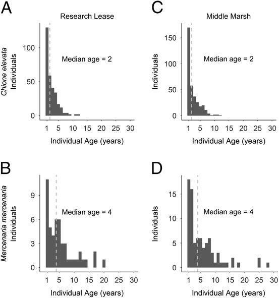
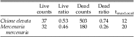
At Research Lease, 37 live and 503 dead right valves of C. elevata were collected; the ratio of left to right C. elevata valves was 0.86. The oldest C. elevata was 12 years old (tmaxLocal). All aged C. elevata had a mean age of 2.1 years, which rose to 2.5 years when individuals aged <1 were excluded (Fig. 2A, B). Median C. elevata age was 2 years regardless of whether individuals aged <1 were excluded. We collected 32 live and 180 dead right valves of M. mercenaria; the ratio of left to right M. mercenaria valves was 1.12. The oldest M. mercenaria was 20 years old (tmaxLocal). All aged M. mercenaria had a mean age of 2.5 years, which rose to 5.5 years when individuals aged <1 were excluded (Fig. 2A, B). Median M. mercenaria age was 0 years when individuals aged <1 were included and 4 years when individuals aged <1 were excluded.
Age frequency distributions (AFDs) for Chione elevata and Mercenaria mercenaria collected from Research Lease and Middle Marsh. AFDs include all live-collected individuals, and all dead right valves ≥1 year of age (if age could be determined for that individual). Gray dashed lines indicate median ages. A, Research Lease C. elevata. B, Research Lease M. mercenaria. C, Middle Marsh C. elevata. D, Middle Marsh M. mercenaria. See Fig. 1 for sites and Supplementary Figs. 1 and 2 for size frequency distributions and size-at-age data, respectively.

At Middle Marsh, 41 live and 542 dead right valves of C. elevata were collected; the ratio of right to left C. elevata valves was 0.92. The oldest C. elevata collected at Middle Marsh was 12 years old (tmaxLocal). All aged C. elevata had a mean age of 2.5 years, which rose to 2.6 years when individuals aged <1 were excluded (Fig. 2C, D). Median C. elevata age was 1 year when individuals aged <1 were included and 2 years when individuals aged <1 were excluded. We collected 45 live and 409 dead right valves of M. mercenaria from Middle Marsh; the ratio of left to right M. mercenaria valves was 1.04. The oldest M. mercenaria collected at Middle Marsh was 28 years old (tmaxLocal). All aged M. mercenaria had a mean age of 2.5 years, which rose to 5.3 years when individuals aged <1 were excluded (Fig. 2C, D). Median M. mercenaria age was 0 years when individuals aged <1 were included and 4 years when individuals aged <1 were excluded.
Mortality Rates
Mortality rates remained fairly consistent for C. elevata regardless of calculation method; instantaneous mortality rate Z ranged from 0.43 to 0.49 at Research Lease and from 0.43 to 0.50 at Middle Marsh (Table 1). The similarity is to be expected for the three calculations based on tmax values, as maximum ages differed by only 1 year. Mortality rates based on C. elevata’s AFD were also close to mortality rates based on tmax values, suggesting that the maximum ages represent the population well and that the AFDs are reasonably representative of a population with tmax=12. In contrast, mortality rates for M. mercenaria varied widely depending upon the calculation method; Z ranged from 0.07 for tmaxGlobal to 0.28 for tmaxLocal at Research Lease, a fourfold increase. This variation is unsurprising, given that tmaxGlobal is more than twice tmaxRegional and three to five times greater than tmaxLocal. As with C. elevata, mortality rates based on M. mercenaria’s AFDs were similar to those based on tmaxLocal, indicating that the distributions are representative of populations with tmax=20 at Research Lease and tmax=28 at Middle Marsh.
Life spans and mortality rates of Mercenaria mercenaria and Chione elevata from the Research Lease and Middle Marsh: Z is the instantaneous mortality rate, calculated via eq. (1) for the various tmax values and via eq. (3) for the age-frequency distributions (AFDs). tmaxGlobal represents the species-wide maximum age; tmaxRegional represents the regional maximum age; tmaxLocal represents the age of the oldest individual of each species collected from each site.

Life Span Bias and Observed Discordance
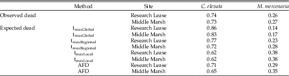
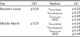
The expected dead ratios of C. elevata to M. mercenaria calculated from the annualized mortality rate and the standing live abundance ranged from 6.14 predicted from tmaxGlobal at Research Lease to 1.63 from tmaxLocal at both Middle Marsh and Research Lease (Table 2). The observed dead ratio of C. elevata to M. mercenaria rose between the living assemblage and the death assemblage from 1.2 to 2.8 at Research Lease and 0.92 to 2.7 at Middle Marsh. The direction of the shift in proportional abundance seen in the OD (positive for C. elevata and negative for M. mercenaria) was the same as the direction of the shift predicted by LB using all calculation methods (Table 3). This result supports hypothesis 1, that C. elevata should be overrepresented in the death assemblage compared with its standing live abundance. Additionally, Middle Marsh exhibited a shift in rank order abundance between C. elevata and M. mercenaria; there were fewer C. elevata than M. mercenaria individuals in the living assemblage, and more C. elevata than M. mercenaria individuals in the death assemblage.
Observed and expected dead ratios of Mercenaria mercenaria and Chione elevata. Abbreviations as in Table 1. Observed dead ratios are the portion of each species collected dead from each site. Expected dead ratios reflect the proportion of each species that should be found in the death assemblage based on the annualized mortality rate and the standing live abundance of each species.

Observed discordance (OD; observed dead proportional abundance − observed live proportional abundance) and life span bias (LB; expected dead proportional abundance − live proportional abundance) for Mercenaria mercenaria and Chione elevata. Abbreviations as in Table 1. OD is the observed change in proportional abundance of each species between the living and death assemblages. LB is the amount that the proportional abundance of each species is expected to change in the death assemblage compared with the living community. In each case, OD and LB were positive for C. elevata (signifying an increase in proportional abundance in the death assemblage) and negative by the same amount for M. mercenaria (indicating a decrease in proportional abundance in the death assemblage).

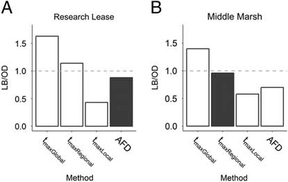
The best predictor of OD at Research Lease was the AFD, which predicted 88% of discordance, followed by tmaxRegional, which overpredicted discordance by 14% (Fig. 3). The best predictor of OD at Middle Marsh was tmaxRegional, which predicted 96% of discordance, followed by the AFD, which predicted 70% of discordance. Thus, hypothesis 2 was supported, and hypothesis 3 was partially supported; the AFD best predicted discordance at Research Lease and tmaxGlobal overpredicted discordance at both sites, by 63% at Research Lease and 40% at Middle Marsh. However, tmaxRegional predicted OD better at both sites than tmaxLocal, which predicted 43% of discordance at Research Lease and 58% at Middle Marsh.
Proportion of observed discordance (OD) explainable by life span bias (LB) for all methods of calculating mortality rate. Dark gray bars represent the best predictor of OD at each site. The dashed line indicates a perfect match between LB and OD (LB/OD=1). A, The best predictor of life span bias at Research Lease was the age-frequency distribution (AFD). B, The best predictor of life span bias at Middle Marsh was tmaxRegional. See Fig. 1 for sites.

Discussion
Life span bias can predict the observed discordance in proportional abundance between the living and death assemblages. Estimates of life span derived from local (AFD) and regional age data predicted this observed discordance better than global age data, and the continued study of life span bias using local life span information will be necessary for refining our understanding of death assemblage fidelity.
Local Life Span Data Better Predict Discordance
Kidwell and Rothfus (Reference Kidwell and Rothfus2010) used global life spans to mitigate underestimates of maximum life spans that could result from insufficient local sampling. However, we found that calculations of LB based on tmaxGlobal overestimated OD in our assemblages, which we attribute to differences in geographic and environmental context (and thus in population demographics) between our sample sites and those that produced tmaxGlobal. Life spans are better known for high-latitude bivalves (Kidwell and Rothfus Reference Kidwell and Rothfus2010), and bivalve life span increases with latitude (Vakily Reference Vakily1992; Buick and Ivany Reference Buick and Ivany2004; Moss et al. Reference Moss, Ivany, Judd, Cummings, Bearden, Kim, Artruc and Driscoll2016). Therefore, global maximum ages for geographically wide-ranging species will primarily represent longer-lived, high-latitude populations and species, which may generate misleading estimates of life span bias on OD for lower-latitude assemblages.
In this study, the latitudinal variation in M. mercenaria life span data explains nearly all differences in the predictive power of the various mortality rates. The oldest recorded M. mercenaria is a 106-year-old individual from Cape Cod, Massachusetts (Ridgway et al. Reference Ridgway, Richardson, Enos, Ungvari, Austad, Philipp and Csiszar2011), nearly 7° north of our study sites. The global maximum age is ~230% greater than tmaxRegional and ~380–530% greater than tmaxLocal, and tmaxGlobal overestimated OD at both North Carolina study sites. In contrast to M. mercenaria, C. elevata tmax values varied only ~10% at the study sites, because both the global and regional maximum ages for C. elevata derive from the same individual, collected at Research Lease (Edie and Surge Reference Edie and Surge2013). However, just as the high-latitude M. mercenaria overestimated OD in North Carolina, C. elevata is at the northern extent of its range in North Carolina (Roopnarine and Vermeij Reference Roopnarine and Vermeij2000), and the tmax values from this study may be inappropriate for estimates of life span bias in the lower-latitude portions of C. elevata’s range: Florida, the Gulf Coast, or northern Central America. Indeed, data from south Florida indicate an approximately 4-year life span (Moore and Lopez Reference Moore and Lopez1969), less than half the North Carolina maximum age (12 years, this study). The latitudinal variation in life span for both M. mercenaria and C. elevata demonstrates that the geographic context of known life spans should be accounted for in assessments of life span bias, and in cases where local tmax differs from global tmax, local life spans should always be used.
Kidwell and Rothfus (Reference Kidwell and Rothfus2010) stated that consistent underestimation of life spans would not change the expected proportions of species in death assemblages and therefore the proportion of OD that could be explained by LB. This study indicated that, due to variation in life span across a species range, global maximum age may instead overestimate the species life span in a local area, whereas insufficient sampling would necessarily underestimate life span. Moreover, due to the wide variation in life span among families and genera (Moss et al. Reference Moss, Ivany, Judd, Cummings, Bearden, Kim, Artruc and Driscoll2016: Supplemental Data), median life span data from confamilials and congeners may over- or underestimate life span. This combined over- and underestimation produced assemblage-level LB estimates that bear little resemblance to OD instead of uniformly decreasing life span bias. Over whole assemblages, LB was not a powerful predictor of OD (Kidwell and Rothfus Reference Kidwell and Rothfus2010), a result that contrasts with our analysis of two species using locally determined mortality rates.
Concern that local maximum ages would underestimate life span bias due to undersampling of the assemblages (Kidwell and Rothfus Reference Kidwell and Rothfus2010) is only partially borne out by the results here. Calculations based on tmaxLocal underestimated but still predicted large proportions of the OD (0.43–0.58; Fig. 3) at both sites. However, the AFD, a local mortality rate estimator, better predicted OD than tmaxLocal at both sites (0.70–0.88; Fig. 3) and was the best predictor at Research Lease. Regional maximum ages predicted OD almost exactly at Middle Marsh (LB/OD=0.96). The 46-year-old M. mercenaria (tmaxRegional) was collected less than 25 km from Middle Marsh (Peterson et al. Reference Peterson, Summerson and Duncan1984) and therefore likely estimated the “true” local maximum age of individuals within the assemblage at Middle Marsh. Though local maximum ages did underestimate OD, AFD and regional maximum ages predicted OD better than global maximum ages did.
Extensive sampling to collect a representative AFD or targeted sampling (sensu Ottens et al. Reference Ottens, Dietl, Kelley and Stanford2012) for larger (and presumably older) individuals ensures local maximum ages are the most appropriate method for evaluating life span bias. However, when local sampling is insufficient, regional maximum ages can sometimes be substituted. Regional tmax overestimated OD for Research Lease by ~14%, which highlights the importance of defining an appropriate region when substituting tmaxRegional for tmaxLocal. Research Lease is less than 130 km from Middle Marsh, and the habitats are similar, though not identical. Both Research Lease and Middle Marsh are back-barrier tidal flat habitats, but Research Lease is unvegetated, and Middle Marsh is vegetated with seagrass. The regional maximum age for M. mercenaria was appropriate for Middle Marsh but not for Research Lease, whereas the regional maximum age for C. elevata was similar to the maximum age at both sites. An appropriate regional scale will likely depend upon latitude, environment, and even the target species, and must be chosen with care.
Finally, and more broadly, using median life spans of congeners, families, or all bivalves to estimate life spans of species can be misleading. Life span estimates available in the literature are incomplete and selective, and many regions and taxa are greatly underrepresented. Knowing the extent of this underrepresentation is important, because life span—a fundamental life-history trait that exhibits considerable variation both within and among species—is determined by many factors. Some of these factors are attributes of species—body size and metabolic rates, for example—whereas others are properties of the environment—availability of nutrients, predation pressure, temperature, and so on. Any analysis of life span bias based on median life spans of congeners or confamilials, or even global maximum ages, cannot control for this critical underlying natural variability. Our results suggest that local to regional, species-specific data can account for the interaction of species traits with their environment to provide a more appropriate test of the life span bias hypothesis.
Potential Confounding Biases in Species Ratios
A number of factors other than life span can potentially alter the proportional abundance of a species in a death assemblage. The methods we used in this study were designed to minimize the impact of these factors and isolate life span bias.
Living assemblages were more seasonally variable than death assemblages (Supplementary Table 1); we therefore used several methods to ensure adequate sampling of live M. mercenaria and C. elevata. First, Middle Marsh was sampled over multiple seasons to compensate for small sample sizes and reduce the influence of temporal variability on the observed live ratios. Second, juveniles, which have higher mortality rates and more seasonal abundance fluctuations than adults, were excluded with the 5-mm mesh sieve (Kidwell Reference Kidwell2001, Reference Kidwell2002). Third, temporal variability in the living assemblage is not as severe a problem for long-lived species, such as M. mercenaria and C. elevata, as it is for shorter-lived opportunists (Kidwell and Rothfus Reference Kidwell and Rothfus2010). The patchy spatial distribution of these species, especially M. mercenaria, could have caused a bias similar to that created by temporal variability, but this problem also was mitigated by multiple sampling trips at Middle Marsh and collecting multiple spatially dispersed bulk samples at both sites (Bennington and Rutherford Reference Bennington and Rutherford1999).
If the death assemblages were dominated by populations with different maximum ages or AFDs due to time averaging of material representing different climates or environments, their comparison with the living assemblages would be inappropriate. Though we did not date the death assemblage, back-barrier environments can have time averaging that spans centuries or millennia (Olszewski and Kaufman Reference Olszewski and Kaufman2015; Dominguez et al. Reference Dominguez, Kosnik, Allen, Hua, Jacob, Kaufman and Whitacre2016; Tomašových et al. Reference Tomašových, Gallmetzer, Haselmair, Kaufman, Vidović and Zuschin2017; Albano et al. Reference Albano, Gallmetzer, Haselmair, Tomašových, Stachowitsch and Zuschin2018). However, death assemblages are usually dominated by the newest cohorts (see Kidwell Reference Kidwell2013), and even several centuries ago, it is unlikely that North Carolina sea-surface temperatures differed enough to change maximum ages appreciably (Shearman and Lentz Reference Shearman and Lentz2010; Cléroux et al. Reference Cléroux, Debret, Cortijo, Duplessy, Dewilde, Reijmer and Massei2012). It is unlikely that our death assemblage includes many individuals from radically different environmental contexts.
Species potentially can experience differential postmortem transport into or out of habitat, which would alter their ratios in the death assemblage. However, transport primarily affects individuals <1 mm (Kidwell Reference Kidwell2002), which were excluded by the sieve size we used, and samples were collected from low-energy back-barrier areas, further reducing the potential for transport bias (Warme Reference Warme1969; Miller Reference Miller1988). Finally, there was little difference in the total number of left and right valves for either species at either site, further evidence against differential transport (Kornicker et al. Reference Kornicker, Wise and Wise1963; Chattopadhyay et al. Reference Chattopadhyay, Rathie and Das2013).
Though the target taxa were chosen to minimize preservation biases based on durability and exposure to postmortem alteration, unknown differences in their preservation potential could influence death assemblage ratios. Individuals <5 mm were excluded from the data, so our analysis considers only the durable size classes likely to persist in death assemblages (Kidwell Reference Kidwell2002). Both species are thick-shelled venerids, so their durability was assumed to be roughly similar. Both species are also infaunal, and valves were sampled from the taphonomically active zone from similar back-barrier environments at both sites, so vulnerability to postmortem alteration was also assumed to be similar (Davies et al. Reference Davies, Powell and Stanton1989; Tomašových et al. Reference Tomašových, Kidwell and Barber2016). However, if M. mercenaria and C. elevata differ in their durability or their vulnerability to postmortem alteration, their death assemblage might be skewed in favor of either species.
Anthropogenic impacts on M. mercenaria, specifically, might have reduced its overall abundance in both the living assemblages and death assemblages by removing whole individuals from the system. Mercenaria mercenaria has been harvested for human consumption in North Carolina for at least 1500 years (Claassen Reference Claassen1986a, Reference Claassenb), whereas C. elevata is not harvested in the southeastern United States. To reduce potential bias, samples were collected from sites that minimize harvest impact on the local populations. Commercial harvest of M. mercenaria is permitted at Middle Marsh using nonmechanical methods only (North Carolina Division of Marine Fisheries n.d.), and it is completely barred at Research Lease.
In short, over entire assemblages, other biasing factors are rarely equal, but the targeted taxa and design of this study were intended to minimize other major factors that might contribute to discordance between live and dead proportional abundances. When other biases were held approximately constant for M. mercenaria and C. elevata, life span bias explained most of the discordance between live and dead proportional abundances.
Utility of Accounting for Life Span Bias in Conservation Paleobiology
One common tool used by conservation paleobiologists to assess anthropogenic impacts on ecosystems is the analysis of live–dead agreement (e.g., see Albano and Sabelli Reference Albano and Sabelli2011; Casey et al. Reference Casey, Dietl, Post and Briggs2014; Negri et al. Reference Negri, Sanfilippo, Basso and Rosso2015; Leshno et al. Reference Leshno, Benjamini and Edelman-Furstenberg2016; Dietl and Smith Reference Dietl and Smith2017; Tomašových and Kidwell Reference Tomašových and Kidwell2017). In such analyses, living assemblages and their death assemblages are assessed for agreement in species composition and rank-order abundance. Low agreement between living and death assemblages (i.e., live–dead discordance or “mismatch”; Kidwell Reference Kidwell2007) may be a predictable result of time averaging; it may indicate death assemblages dominated by old cohorts, multi-environment time averaging, or living assemblages dominated by low-durability species (Tomašových and Kidwell Reference Tomašových and Kidwell2009, Reference Tomašových and Kidwell2010; Kidwell Reference Kidwell2013). If such factors can be eliminated, conservation paleobiologists tend to attribute discordance in species composition and rank order between living assemblages and death assemblages to anthropogenic impact (Kidwell Reference Kidwell2007).
At Middle Marsh, the shift in proportional abundance of M. mercenaria and C. elevata yielded a reversal of rank order, suggesting that life span bias should be considered in live–dead studies. Though rare species are resistant to changes in rank order induced by life span bias (Kidwell and Rothfus Reference Kidwell and Rothfus2010), common species with different life spans may be vulnerable to shifts in rank order based on life span. Under circumstances in which life span bias contributes to shifts in rank order in a live–dead agreement study, tests for anthropogenic disturbance could yield false positives in live–dead discordance. Resources and political will for environmental remediation are often scarce, so it is important that resources are allocated to ecosystems where live–dead disagreement is caused by anthropogenic effects, rather than life span or other biases.
Conclusions and Recommendations
Life span bias can explain discordance between the proportional abundances of living and death assemblages. In our study, the shorter-lived species (C. elevata) was overrepresented in the death assemblage compared with the longer-lived species (M. mercenaria). Global maximum ages led to overestimations of discordance, but estimates improved considerably when life span estimates (using AFDs and regional life spans) more closely reflected the population demographics of the assemblages.
The live–dead mismatch approach has been used by conservationists in identifying species and habitats of conservation concern. However, the reliability and accuracy of live–dead assessments should be checked against known biases—including life span bias. The sampling design of future live–dead studies could include targeted sampling of the largest individuals within a site to estimate the true maximum age within the local population. For instances in which targeted sampling of large individuals is difficult (e.g., dredging or core-based sampling), the largest individuals from across these bulk samples are expected to provide an appropriate local age of the population. If local sampling is thought to be insufficient (e.g., low sample sizes), regional maximum ages can be used, especially if the regional data come from appropriate latitudinal and environmental contexts.
Analyses of life span bias should be conducted, both for entire assemblages and at smaller taxonomic scales, such as the scale used here, to better understand the influence of life span compared with other biases. Reporting cases in which life span bias is small relative to other factors, as well as cases in which life span explains observed discordance, would provide necessary insight into the circumstances under which life span bias alters abundances, ultimately developing a more complete picture of the fidelity of live–dead assemblages.
Supplementary Material
Data available from the Dryad Digital Repository: https://doi.org/10.5061/dryad.3st56j0
Acknowledgments
We thank M. Kosnik and A. Tomašových for their thoughtful and helpful reviews on the article. We also gratefully acknowledge S. Neely, N. Armstrong, E. Baumgardt, J. Burke, P. Capar, K. Cooke, S. Davis, K. Duernberger., S. Durham, B. Kelly, A. Lade, K. Mohr, N. Moore, J. Nester, C. Pierce, R. Ratchford, J. Sime, J. Smith, A. Eisenhart, and C. Visaggi for their time and assistance in the field. Work on this project was funded by the National Science Foundation under grant no. EAR-0755109, the Geological Society of America, and the Paleontological Society.
Appendix: Life Span Bias Calculation
The methods used to calculate life span bias are explained in detail below. Steps are numbered to correspond to the steps referenced in the “Materials and Methods” section. Abundance and tmaxLocal data (Table A1) used in this example are from the University of North Carolina Wilmington Research Lease.
1. Calculate mortality rates for each species:
a. Determine the instantaneous mortality rate, Z using eq. (1) (Hoenig Reference Hoenig1983).
 $$\eqalignno{ & Chione\colon\,{\rm Ln}\left( Z \right){\equals}1.23{\plus}\left[ {{\minus}0.832^{\asterisk}{\rm ln}\left( {12} \right)} \right] \cr & \hskip 15ptZ{\equals}0.43 \cr & {\it Mercenaria}\colon\,{\rm Ln}\left( Z \right){\equals}1.23{\plus}\left[ {{\minus}0.832^{\asterisk}{\rm ln}\left( {20} \right)} \right] \cr & \hskip 15ptZ{\equals}0.28 $$
b. Convert Z to the annualized mortality rate (AMR) using eq. (2).
$$\eqalignno{ & Chione\colon\,{\rm AMR}{\equals}1{\hbox -}{\rm e}^{{{\minus}{\rm Z}}} {\equals}0.35 \cr & Mercenaria\colon\,{\rm AMR}{\equals}1{\hbox -}{\rm e}^{{{\minus}{\rm Z}}} {\equals}0.25 $$
2. Determine the number of individuals of each species that should die and be added to the death assemblage yearly:


a. Multiply live abundance by annualized mortality rate:
$$\eqalignno{ & Chione\colon\,{\rm }\left( {37^{\asterisk}0.35} \right){\equals}13.0 \cr & Mercenaria\colon\left( {32^{\asterisk}0.25} \right){\equals}8.0 $$
b. Convert to proportions of the total, the expected dead:
$$\eqalignno{ & Chione\colon\,0.62 \cr & Mercenaria\colon\,0.38 $$
c. Assuming constant mortality over time, the proportion of Chione and Mercenaria in the death assemblage should remain the same as the proportion of individuals added each year. Thus, the expected ratio of dead Chione to dead Mercenaria in the entire death assemblage will be 0.62:0.38.


3. Determine the expected difference between the live ratios and the dead ratios owing to the difference in life span between Chione and Mercenaria, called life span bias (LB) by Kidwell and Rothfus (Reference Kidwell and Rothfus2010).
a. Subtract the observed live ratio from the expected dead ratio.
$$\eqalignno{ & Chione\colon\,{\rm }\left( {0.62{\minus}0.53} \right){\equals}0.09 \cr & Mercenaria\colon\,{\rm }\left( {0.38{\minus}0.47} \right){\equals}{\minus}0.09 $$
b. Chione’s positive value indicates that the proportional abundance is expected to rise from the living assemblage to the death assemblage. Mercenaria’s negative value indicates that it is expected to decrease in proportional abundance from live to dead.

4. Determine the actual difference between the observed live and the observed dead ratios of Chione and Mercenaria, called observed discordance both in this study and by Kidwell and Rothfus (Reference Kidwell and Rothfus2010).
a. Subtract the observed live ratio from the observed dead ratio.
$$\eqalignno{ & Chione\colon\,\left( {0.74{\minus}0.53} \right){\equals}0.21 \cr & Mercenaria\colon\,\left( {0.26{\minus}0.47} \right){\equals}{\minus}0.21 $$
b. Based on the difference in life span, Chione should have increased in the death assemblage by 0.09, according to the mortality rates calculated from tmaxLocal. The actual increase was 0.21. Mercenaria should have decreased by 0.09. The actual decrease was 0.21.

5. Finally, the percentage of the observed discordance that is explainable by life span bias is calculated by dividing life span bias by observed discordance (LB/OD):
 $$\eqalignno{ & Chione{\equals}0.09\,/\,0.21{\equals}43\,\%\, \cr & Mercenaria{\equals}{\minus}0.09\,/\,{\minus}0.21{\equals}43\,\%\, $$
Chione elevata and Mercenaria mercenaria abundance from Research Lease.

Local life span differences can explain ~43% of the observed live–dead discordance between Chione and Mercenaria at Research Lease. Note that step 5 in our method differs substantially from Kidwell and Rothfus’s (Reference Kidwell and Rothfus2010) method for quantifying how much life span bias contributes to observed discordance, because we analyzed only two species. A study following these methods for an entire assemblage, rather than just two species, should refer to the methods in Kidwell and Rothfus (Reference Kidwell and Rothfus2010) rather than reproducing our method.