1 Introduction
Since formulation of the mean-field dynamo approach in a seminal paper by Steenbeck, Krause and Rädler in 1966 (Steenbeck, Krause & Rädler Reference Steenbeck, Krause and Rädler1966; Roberts & Stix Reference Roberts and Stix1971; Krause & Rädler Reference Krause and Rädler1980), the theories of solar magnetic fields have been actively developing during last 50 years (Moffatt Reference Moffatt1978; Parker Reference Parker1979; Krause & Rädler Reference Krause and Rädler1980; Zeldovich, Ruzmaikin & Sokoloff Reference Zeldovich, Ruzmaikin and Sokoloff1983; Ossendrijver Reference Ossendrijver2003; Brandenburg & Subramanian Reference Brandenburg and Subramanian2005; Rüdiger, Kitchatinov & Hollerbach Reference Rüdiger, Kitchatinov and Hollerbach2013). A well-known point of view on origin of the large-scale solar magnetic field is that the field is generated in the solar convective zone by a combine action of helical convective turbulent motions and large-scale non-uniform rotation (so called
 $\unicode[STIX]{x1D6FC}\unicode[STIX]{x1D6FA}$
or
 $\unicode[STIX]{x1D6FC}^{2}\unicode[STIX]{x1D6FA}$
mean-field dynamo). This large-scale magnetic field causes the 11-year solar cyclic activity.
However, the observed solar activity is associated with strongly concentrated magnetic fields such as sunspots with the characteristic spatial scale of the order of solar super-granulation (approximately
 $10^{4}$
km). On the other hand, the mean-field dynamo generates smooth large-scale magnetic fields with the characteristic scale of the order of the solar radius (approximately
 $10^{6}$
km). Thus it was not clear for many years how the mean-field dynamo relates to with the sunspots. One of the suggested mechanisms of magnetic spot formation is the magnetic buoyancy instability investigated by Parker in 1966 (Parker Reference Parker1966, Reference Parker1979; Priest Reference Priest1982). This instability is excited when the characteristic scale of original magnetic field variation is smaller than the density stratification height. Therefore, in a strongly density stratified convective zone where the density varies in radial direction by 7 orders of magnitude, this instability is only excited when the initial magnetic field is already strongly non-uniform.
Another mechanism of magnetic spot formation is related to the negative effective magnetic pressure instability (NEMPI), which can be excited even for uniform initial large-scale magnetic field (Kleeorin, Rogachevskii & Ruzmaikin Reference Kleeorin, Rogachevskii and Ruzmaikin1989, Reference Kleeorin, Rogachevskii and Ruzmaikin1990). The mechanism of this instability is based on the suppression of total (hydrodynamic and magnetic) turbulent pressure by a large-scale magnetic field. This effect can be understood as a negative contribution of turbulence to the effective mean magnetic pressure (the sum of non-turbulent and turbulent contributions). At large fluid and magnetic Reynolds numbers this turbulent contribution becomes large and a large-scale instability can be excited, redistributing the magnetic flux produced by the mean-field dynamo. NEMPI has been studied analytically using the mean-field approach (Kleeorin, Mond & Rogachevskii Reference Kleeorin, Mond and Rogachevskii1993, Reference Kleeorin, Mond and Rogachevskii1996; Kleeorin & Rogachevskii Reference Kleeorin and Rogachevskii1994; Rogachevskii & Kleeorin Reference Rogachevskii and Kleeorin2007) and numerically using mean-field simulations (Brandenburg, Kleeorin & Rogachevskii Reference Brandenburg, Kleeorin and Rogachevskii2010; Kemel et al. Reference Kemel, Brandenburg, Kleeorin, Mitra and Rogachevskii2012, Reference Kemel, Brandenburg, Kleeorin, Mitra and Rogachevskii2013; Brandenburg et al. Reference Brandenburg, Gressel, Jabbari, Kleeorin and Rogachevskii2014; Brandenburg, Rogachevskii & Kleeorin Reference Brandenburg, Rogachevskii and Kleeorin2016), large-eddy simulations (Käpylä et al. Reference Käpylä, Brandenburg, Kleeorin, Mantere and Rogachevskii2012, Reference Käpylä, Brandenburg, Kleeorin, Käpylä and Rogachevskii2016) and direct numerical simulations (Brandenburg et al. Reference Brandenburg, Kemel, Kleeorin, Mitra and Rogachevskii2011, Reference Brandenburg, Kemel, Kleeorin and Rogachevskii2012; Brandenburg, Kleeorin & Rogachevskii Reference Brandenburg, Kleeorin and Rogachevskii2013; Warnecke et al. Reference Warnecke, Losada, Brandenburg, Kleeorin and Rogachevskii2013, Reference Warnecke, Losada, Brandenburg, Kleeorin and Rogachevskii2016; Mitra et al. Reference Mitra, Brandenburg, Kleeorin and Rogachevskii2014; Jabbari et al. Reference Jabbari, Brandenburg, Mitra, Kleeorin and Rogachevskii2016).
Predictions of solar activity is a subject of active investigation where various methods, including the mean-field dynamo models, have been used (Dikpati, De Toma & Gilman Reference Dikpati, De Toma and Gilman2006; Bushby & Tobias Reference Bushby and Tobias2007; Choudhuri, Chatterjee & Jiang Reference Choudhuri, Chatterjee and Jiang2007; Kane Reference Kane2007; Obridko & Shelting Reference Obridko and Shelting2008; De Jager & Duhau Reference De Jager and Duhau2009; Tlatov Reference Tlatov2009, Reference Tlatov2015; Kitiashvili & Kosovichev Reference Kitiashvili and Kosovichev2011; Pesnell Reference Pesnell2012; Usoskin Reference Usoskin2017). However, the improving of the solar activity forecast is still a subject of numerous discussions.
In the present study we apply a nonlinear mean-field dynamo model and a budget equation for the dynamics of Wolf numbers (Kleeorin et al.
Reference Kleeorin, Safiullin, Kleeorin, Porshnev, Rogachevskii and Sokoloff2016) to predict solar activity. This budget equation is related to a mechanism of formation of sunspots based on NEMPI. The dynamo model includes the algebraic and dynamic quenching of the
 $\unicode[STIX]{x1D6FC}$
effect. To predict solar activity on the time scale of one month we use a method based on a combination of the numerical solution of the nonlinear mean-field dynamo equations (Kleeorin et al.
Reference Kleeorin, Safiullin, Kleeorin, Porshnev, Rogachevskii and Sokoloff2016) and the artificial neural network approach (Fessant, Pierret & Lantos Reference Fessant, Pierret and Lantos1996; Conway Reference Conway1998; Hagan, Demuth & Beale Reference Hagan, Demuth and Beale2016).
2 Nonlinear dynamo model
To study nonlinear evolution of the large-scale magnetic field, we use the induction equation in spherical coordinates
 $(r,\unicode[STIX]{x1D703},\unicode[STIX]{x1D719})$
for an axisymmetric mean magnetic field,
 $\overline{\boldsymbol{B}}=\overline{B}_{\unicode[STIX]{x1D719}}\boldsymbol{e}_{\unicode[STIX]{x1D719}}+\unicode[STIX]{x1D735}\boldsymbol{\times }(\overline{\unicode[STIX]{x1D608}}\boldsymbol{e}_{\unicode[STIX]{x1D719}})$
. We investigate the dynamo action in a thin convective shell. To take into account strong variation of the plasma density in the radial direction, we average the equations for the mean toroidal field
 $\overline{B}_{\unicode[STIX]{x1D719}}$
and the magnetic potential
 $\overline{\unicode[STIX]{x1D608}}$
of the mean poloidal field over the depth of the convective shell, so that all quantities are functions of colatitude
 $\unicode[STIX]{x1D703}$
. We neglect the curvature of the convective shell and replace it by a flat slab. These simplifications yield the non-dimensional mean-field dynamo equations (Kleeorin et al.
Reference Kleeorin, Kuzanyan, Moss, Rogachevskii, Sokoloff and Zhang2003):
 $$\begin{eqnarray}\displaystyle & \displaystyle \frac{\unicode[STIX]{x2202}\overline{B}_{\unicode[STIX]{x1D719}}}{\unicode[STIX]{x2202}t}=GD\sin \unicode[STIX]{x1D703}\frac{\unicode[STIX]{x2202}\overline{\unicode[STIX]{x1D608}}}{\unicode[STIX]{x2202}\unicode[STIX]{x1D703}}+\frac{\unicode[STIX]{x2202}^{2}\overline{B}_{\unicode[STIX]{x1D719}}}{\unicode[STIX]{x2202}\unicode[STIX]{x1D703}^{2}}-\unicode[STIX]{x1D707}^{2}\overline{B}_{\unicode[STIX]{x1D719}}, & \displaystyle\end{eqnarray}$$
 $$\begin{eqnarray}\displaystyle & \displaystyle \frac{\unicode[STIX]{x2202}\overline{\unicode[STIX]{x1D608}}}{\unicode[STIX]{x2202}t}=\unicode[STIX]{x1D6FC}\overline{B}_{\unicode[STIX]{x1D719}}+\frac{\unicode[STIX]{x2202}^{2}\overline{\unicode[STIX]{x1D608}}}{\unicode[STIX]{x2202}\unicode[STIX]{x1D703}^{2}}-\unicode[STIX]{x1D707}^{2}\overline{\unicode[STIX]{x1D608}}, & \displaystyle\end{eqnarray}$$
where the terms,
 $-\unicode[STIX]{x1D707}^{2}\overline{B}_{\unicode[STIX]{x1D719}}$
and
 $-\unicode[STIX]{x1D707}^{2}\overline{\unicode[STIX]{x1D608}}$
, in (2.1) and (2.2) describe turbulent diffusion of the mean magnetic field in the radial direction, the parameter
 $G=\unicode[STIX]{x2202}\unicode[STIX]{x1D6FA}/\unicode[STIX]{x2202}r$
determines the differential rotation and
 $D$
is the dynamo number defined below. The parameter
 $\unicode[STIX]{x1D707}$
is determined by the equation:
 $$\begin{eqnarray}\displaystyle \int _{2/3}^{1}\frac{\unicode[STIX]{x2202}^{2}\overline{B}_{\unicode[STIX]{x1D719}}}{\unicode[STIX]{x2202}r^{2}}\,\text{d}r=-\frac{\unicode[STIX]{x1D707}^{2}\overline{B}_{\unicode[STIX]{x1D719}}}{3}. & & \displaystyle\end{eqnarray}$$
In (2.1)–(2.3) the length is measured in units of radius
 $R_{\odot }$
, time is measured in units of the turbulent magnetic diffusion time
 $R_{\odot }^{2}/\unicode[STIX]{x1D702}_{T}$
, the differential rotation
 $\unicode[STIX]{x1D6FF}\unicode[STIX]{x1D6FA}$
is measured in units of the maximal value of the angular velocity
 $\unicode[STIX]{x1D6FA}$
, and
 $\unicode[STIX]{x1D6FC}$
is measured in units of the maximum value
 $\unicode[STIX]{x1D6FC}_{0}$
of the kinetic part of the
 $\unicode[STIX]{x1D6FC}$
-effect. The toroidal mean magnetic field,
 $\overline{B}_{\unicode[STIX]{x1D719}}$
is measured in the units of the equipartition field
 $\overline{B}_{\text{eq}}=u_{0}\sqrt{4\unicode[STIX]{x03C0}\overline{\unicode[STIX]{x1D70C}}_{\ast }}$
, and the vector potential of the mean poloidal field
 $\overline{\unicode[STIX]{x1D608}}$
is measured in units of
 $R_{\unicode[STIX]{x1D6FC}}R_{\odot }\overline{B}_{\text{eq}}$
. The density
 $\overline{\unicode[STIX]{x1D70C}}$
is normalized by its value
 $\overline{\unicode[STIX]{x1D70C}}_{\ast }$
at the bottom of the convective zone, and the integral scale of the turbulent motions
 $\ell _{0}$
and turbulent velocity
 $u_{0}$
at the scale
 $\ell _{0}$
are measured in units of their maximum values through the convective region. The magnetic Reynolds number
 $\text{Rm}=\ell _{0}u_{0}/\unicode[STIX]{x1D702}$
is defined using these maximal values, and the turbulent magnetic diffusivity is
 $\unicode[STIX]{x1D702}_{T}=\ell _{0}u_{0}/3$
. Here
 $\unicode[STIX]{x1D702}$
is the magnetic diffusion coefficient due to electrical conductivity of the plasma. The dynamo number is defined as
 $D=R_{\unicode[STIX]{x1D6FC}}R_{\unicode[STIX]{x1D714}}$
, where
 $R_{\unicode[STIX]{x1D6FC}}=\unicode[STIX]{x1D6FC}_{0}R_{\odot }/\unicode[STIX]{x1D702}_{T}$
and
 $R_{\unicode[STIX]{x1D714}}=(\unicode[STIX]{x1D6FF}\unicode[STIX]{x1D6FA})\,R_{\odot }^{2}/\unicode[STIX]{x1D702}_{T}$
. Equations (2.1) and (2.2) describe the dynamo waves propagating from the central latitudes towards the equator when the dynamo number is negative. The radius
 $r$
varies from
 $2/3$
to
 $1$
inside the convective shell, so that the value
 $\unicode[STIX]{x1D707}=3$
corresponds to a convective zone with a thickness of approximately 1/3 of the radius.
The total
 $\unicode[STIX]{x1D6FC}$
effect is defined as the sum of the kinetic,
 $\unicode[STIX]{x1D6FC}^{v}=\unicode[STIX]{x1D712}^{v}\unicode[STIX]{x1D719}_{v}(\overline{B})$
, and magnetic,
 $\unicode[STIX]{x1D6FC}^{m}=\unicode[STIX]{x1D712}^{c}\unicode[STIX]{x1D719}_{m}(\overline{B})$
, parts:
 $$\begin{eqnarray}\displaystyle \unicode[STIX]{x1D6FC}(r,\unicode[STIX]{x1D703})=\unicode[STIX]{x1D712}^{v}\unicode[STIX]{x1D719}_{v}(\overline{B})+\unicode[STIX]{x1D712}^{c}\unicode[STIX]{x1D719}_{m}(\overline{B}), & & \displaystyle\end{eqnarray}$$
where
 $\unicode[STIX]{x1D712}^{v}=-(\unicode[STIX]{x1D70F}_{0}/3)\,\overline{\boldsymbol{u}\boldsymbol{\cdot }(\unicode[STIX]{x1D735}\boldsymbol{\times }\boldsymbol{u})}$
,
 $\,\unicode[STIX]{x1D712}^{c}=(\unicode[STIX]{x1D70F}_{0}/12\unicode[STIX]{x03C0}\overline{\unicode[STIX]{x1D70C}})\,\overline{\boldsymbol{b}\boldsymbol{\cdot }(\unicode[STIX]{x1D735}\boldsymbol{\times }\boldsymbol{b})}$
,
 $\unicode[STIX]{x1D70F}_{0}$
is the correlation time of the turbulent velocity field,
 $\boldsymbol{u}$
and
 $\boldsymbol{b}$
are the velocity and magnetic fluctuations, respectively. We adopt the standard profile of the kinetic part of the
 $\unicode[STIX]{x1D6FC}$
effect:
 $\unicode[STIX]{x1D6FC}(\unicode[STIX]{x1D703})=\unicode[STIX]{x1D6FC}_{0}\sin ^{3}\unicode[STIX]{x1D703}\cos \unicode[STIX]{x1D703}$
. The magnetic part of the
 $\unicode[STIX]{x1D6FC}$
effect (Pouquet, Frisch & Léorat Reference Pouquet, Frisch and Léorat1976) and density of the magnetic helicity are related to the density of the current helicity
 $\overline{\boldsymbol{b}\boldsymbol{\cdot }(\unicode[STIX]{x1D735}\boldsymbol{\times }\boldsymbol{b})}$
in the approximation of weakly inhomogeneous turbulent convection (Kleeorin & Rogachevskii Reference Kleeorin and Rogachevskii1999). The quenching functions
 $\unicode[STIX]{x1D719}_{v}(\overline{B})$
and
 $\unicode[STIX]{x1D719}_{m}(\overline{B})$
in (2.4) are given by:
 $$\begin{eqnarray}\displaystyle & \displaystyle \unicode[STIX]{x1D719}_{v}(\overline{B})=(1/7)[4\unicode[STIX]{x1D719}_{m}(\overline{B})+3L(\overline{B})], & \displaystyle\end{eqnarray}$$
 $$\begin{eqnarray}\displaystyle & \displaystyle \unicode[STIX]{x1D719}_{m}(\overline{B})=\frac{3}{8\overline{B}^{2}}[1-\arctan (\sqrt{8}\overline{B})/\sqrt{8}\overline{B}], & \displaystyle\end{eqnarray}$$
(Rogachevskii & Kleeorin Reference Rogachevskii and Kleeorin2000, Reference Rogachevskii and Kleeorin2001), where
 $L(\overline{B})=1-16\overline{B}^{2}+128\overline{B}^{4}\ln (1+1/(8\overline{B}^{2}))$
. The quenching functions have the following asymptotics:
 $\unicode[STIX]{x1D719}_{v}(\overline{B})=1-(48/5)\overline{B}^{2}$
and
 $\unicode[STIX]{x1D719}_{m}(\overline{B})=1-(24/5)\overline{B}^{2}$
for a weak magnetic field,
 $\overline{B}\ll 1$
, while
 $\unicode[STIX]{x1D719}_{v}(\overline{B})=1/(4\overline{B}^{2})$
and
 $\unicode[STIX]{x1D719}_{m}(\overline{B})=3/(8\overline{B}^{2})$
for a strong magnetic field,
 $\overline{B}\gg 1$
, where
 $\unicode[STIX]{x1D712}^{v}$
and
 $\unicode[STIX]{x1D712}^{c}$
are measured in units of the maximal value of the
 $\unicode[STIX]{x1D6FC}$
effect. The function
 $\unicode[STIX]{x1D719}_{v}$
describes the algebraic quenching of the kinetic part of the
 $\unicode[STIX]{x1D6FC}$
effect that is caused by the effects of the mean magnetic field on the electromotive force (Rogachevskii & Kleeorin Reference Rogachevskii and Kleeorin2000, Reference Rogachevskii and Kleeorin2001, Reference Rogachevskii and Kleeorin2004).
We average (2.4) over the depth of the convective zone, so that the first term in the averaged equation is determined by the values taken at the middle part of the convective zone, while in the second term there is a phenomenological parameter
 $\unicode[STIX]{x1D70E}$
:
 $$\begin{eqnarray}\displaystyle \unicode[STIX]{x1D6FC}(\unicode[STIX]{x1D703})=\unicode[STIX]{x1D712}^{v}\unicode[STIX]{x1D719}_{v}(\overline{B})+\unicode[STIX]{x1D70E}\unicode[STIX]{x1D712}^{c}\unicode[STIX]{x1D719}_{m}(\overline{B}),\quad \unicode[STIX]{x1D70E}=\int \left(\frac{\overline{\unicode[STIX]{x1D70C}}(r)}{\overline{\unicode[STIX]{x1D70C}}_{\ast }}\right)^{-1}\,\text{d}r, & & \displaystyle\end{eqnarray}$$
(Zhang et al.
Reference Zhang, Moss, Kleeorin, Kuzanyan, Rogachevskii, Sokoloff, Gao and Xu2012; Kleeorin et al.
Reference Kleeorin, Safiullin, Kleeorin, Porshnev, Rogachevskii and Sokoloff2016), where the densities of the helicities and quenching functions are associated with a middle part of the convective zone. The parameter
 $\unicode[STIX]{x1D70E}>1$
is a free parameter.
The magnetic part
 $\unicode[STIX]{x1D6FC}^{m}$
of the
 $\unicode[STIX]{x1D6FC}$
effect is based on two nonlinearities: the algebraic quenching, given by the function
 $\unicode[STIX]{x1D719}_{m}(\overline{B})$
(Field, Blackman & Chou Reference Field, Blackman and Chou1999; Rogachevskii & Kleeorin Reference Rogachevskii and Kleeorin2000, Reference Rogachevskii and Kleeorin2001) and the dynamic nonlinearity. The function
 $\unicode[STIX]{x1D712}^{c}(\overline{\boldsymbol{B}})$
is determined by a dynamical equation that is derived using the conservation law for magnetic helicity (Kleeorin & Ruzmaikin Reference Kleeorin and Ruzmaikin1982; Gruzinov & Diamond Reference Gruzinov and Diamond1994; Kleeorin, Rogachevskii & Ruzmaikin Reference Kleeorin, Rogachevskii and Ruzmaikin1995):
 $$\begin{eqnarray}\displaystyle \frac{\unicode[STIX]{x2202}\unicode[STIX]{x1D712}^{c}}{\unicode[STIX]{x2202}t}+\unicode[STIX]{x1D735}\boldsymbol{\cdot }\unicode[STIX]{x1D731}+\frac{\unicode[STIX]{x1D712}^{c}}{T}=-\frac{1}{9\unicode[STIX]{x03C0}\unicode[STIX]{x1D702}_{T}\overline{\unicode[STIX]{x1D70C}}_{\ast }}(\boldsymbol{{\mathcal{E}}}\boldsymbol{\cdot }\overline{\boldsymbol{B}}), & & \displaystyle\end{eqnarray}$$
where
 $\unicode[STIX]{x1D731}=-\unicode[STIX]{x1D705}_{T}\unicode[STIX]{x1D735}\unicode[STIX]{x1D712}^{c}$
is the turbulent diffusion flux of the density of the magnetic helicity (Kleeorin & Rogachevskii Reference Kleeorin and Rogachevskii1999; Blackman & Field Reference Blackman and Field2000; Kleeorin et al.
Reference Kleeorin, Moss, Rogachevskii and Sokoloff2000, Reference Kleeorin, Kuzanyan, Moss, Rogachevskii, Sokoloff and Zhang2003; Brandenburg & Subramanian Reference Brandenburg and Subramanian2005),
 $\unicode[STIX]{x1D705}_{T}$
is the coefficient of the turbulent diffusion,
 $T=\ell _{0}^{2}/\unicode[STIX]{x1D702}$
is the relaxation time of magnetic helicity and
 $\boldsymbol{{\mathcal{E}}}$
is the mean electromotive force. Since the total magnetic helicity is conserved, the increase of the density of the large-scale magnetic helicity due to the dynamo action, should be compensated by the decrease of the density of the small-scale magnetic helicity. The compensation mechanisms include the dissipation and transport of the density of the magnetic helicity. The dynamical equation (2.8) for the function
 $\unicode[STIX]{x1D712}^{c}(\overline{\boldsymbol{B}})$
in non-dimensional form reads
 $$\begin{eqnarray}\displaystyle \frac{\unicode[STIX]{x2202}\unicode[STIX]{x1D712}^{c}}{\unicode[STIX]{x2202}t}+(T^{-1}+\unicode[STIX]{x1D705}_{T}\unicode[STIX]{x1D707}^{2})\unicode[STIX]{x1D712}^{c}=2\left(\frac{\unicode[STIX]{x2202}\overline{\unicode[STIX]{x1D608}}}{\unicode[STIX]{x2202}\unicode[STIX]{x1D703}}\frac{\unicode[STIX]{x2202}\overline{B}_{\unicode[STIX]{x1D719}}}{\unicode[STIX]{x2202}\unicode[STIX]{x1D703}}+\unicode[STIX]{x1D707}^{2}\overline{\unicode[STIX]{x1D608}}\,\overline{B}_{\unicode[STIX]{x1D719}}\right)-\frac{\unicode[STIX]{x1D6FC}}{\unicode[STIX]{x1D709}}\overline{B}^{2}-\frac{\unicode[STIX]{x2202}}{\unicode[STIX]{x2202}\unicode[STIX]{x1D703}}\left(\overline{B}_{\unicode[STIX]{x1D719}}\frac{\unicode[STIX]{x2202}\overline{\unicode[STIX]{x1D608}}}{\unicode[STIX]{x2202}\unicode[STIX]{x1D703}}-\unicode[STIX]{x1D705}_{T}\frac{\unicode[STIX]{x2202}\unicode[STIX]{x1D712}^{c}}{\unicode[STIX]{x2202}\unicode[STIX]{x1D703}}\right), & & \displaystyle \nonumber\\ \displaystyle & & \displaystyle\end{eqnarray}$$
(Zhang et al. Reference Zhang, Moss, Kleeorin, Kuzanyan, Rogachevskii, Sokoloff, Gao and Xu2012; Kleeorin et al. Reference Kleeorin, Safiullin, Kleeorin, Porshnev, Rogachevskii and Sokoloff2016), where
 $$\begin{eqnarray}\displaystyle \overline{B}^{2}=\unicode[STIX]{x1D709}\left\{\overline{B}_{\unicode[STIX]{x1D719}}^{2}+R_{\unicode[STIX]{x1D6FC}}^{2}\left[\unicode[STIX]{x1D707}^{2}\overline{\unicode[STIX]{x1D608}}^{2}+\left(\frac{\unicode[STIX]{x2202}\overline{\unicode[STIX]{x1D608}}}{\unicode[STIX]{x2202}\unicode[STIX]{x1D703}}\right)^{2}\right]\right\}, & & \displaystyle\end{eqnarray}$$
and
 $\unicode[STIX]{x1D709}=2(\ell _{0}/R_{\odot })^{2}$
. In derivation of (2.9)–(2.10), we average (2.8) over the depth of the convective zone, so that the average value of
 $T^{-1}$
is
 $$\begin{eqnarray}\displaystyle T^{-1}=H^{-1}\int T^{-1}(r)\,\text{d}r\sim \frac{\unicode[STIX]{x1D6EC}_{\ell }R_{\odot }^{2}\unicode[STIX]{x1D702}}{H\ell _{0}^{2}\unicode[STIX]{x1D702}_{T}}, & & \displaystyle\end{eqnarray}$$
where
 $H$
is the depth of the convective zone,
 $\unicode[STIX]{x1D6EC}_{\ell }$
is the characteristic scale of variations
 $\ell _{0}$
and
 $T(r)=(\unicode[STIX]{x1D702}_{T}/R_{\odot }^{2})(\ell _{0}^{2}/\unicode[STIX]{x1D702})$
is the non-dimensional relaxation time of the density of the magnetic helicity. The values
 $\unicode[STIX]{x1D6EC}_{\ell },\,\unicode[STIX]{x1D702},\,\ell _{0}$
in (2.11) are associated with the upper part of the convective zone.
In view of observations, an important parameter of the solar activity is the Wolf number (Gibson Reference Gibson1973; Stix Reference Stix2012),
 $W=10g+f$
, where
 $g$
is the number of sunspot groups and
 $f$
is the total number of sunspots on the visible part of the Sun. This parameter has been measured over three centuries. Based on the idea of NEMPI, we derive a budget equation for the surface density of the Wolf number (Kleeorin et al.
Reference Kleeorin, Safiullin, Kleeorin, Porshnev, Rogachevskii and Sokoloff2016):
 $$\begin{eqnarray}\displaystyle \frac{\unicode[STIX]{x2202}\tilde{W}}{\unicode[STIX]{x2202}t}=I(t,\unicode[STIX]{x1D703})-\frac{\tilde{W}}{\unicode[STIX]{x1D70F}_{s}(\overline{B})}. & & \displaystyle\end{eqnarray}$$
Equation (2.12) includes the rate of production of the surface density of the Wolf number,
 $\tilde{W}(t,\unicode[STIX]{x1D703})$
, caused by the formation of sunspots:
 $$\begin{eqnarray}\displaystyle I(t,\unicode[STIX]{x1D703})=\frac{|\unicode[STIX]{x1D6FE}_{\text{inst}}||\overline{B}-\overline{B}_{\text{cr}}|}{\unicode[STIX]{x1D6F7}_{s}}\unicode[STIX]{x1D6E9}(\overline{B}-\overline{B}_{\text{cr}}), & & \displaystyle\end{eqnarray}$$
and the rate of decay of sunspots,
 $\tilde{W}/\unicode[STIX]{x1D70F}_{s}(\overline{B})$
, where the decay time,
 $\unicode[STIX]{x1D70F}_{s}(\overline{B})$
, of sunspots is discussed below and
 $\unicode[STIX]{x1D6E9}(x)$
is the
 $\unicode[STIX]{x1D6E9}$
function, defined as
 $\unicode[STIX]{x1D6E9}(x)=1$
for
 $x>0$
, and
 $\unicode[STIX]{x1D6E9}(x)=0$
for
 $x\leqslant 0$
.
The growth rate of NEMPI,
 $\unicode[STIX]{x1D6FE}_{\text{inst}}$
, is given by (Rogachevskii & Kleeorin Reference Rogachevskii and Kleeorin2007; Losada et al.
Reference Losada, Brandenburg, Kleeorin, Mitra and Rogachevskii2012; Brandenburg et al.
Reference Brandenburg, Rogachevskii and Kleeorin2016):
 $$\begin{eqnarray}\displaystyle \unicode[STIX]{x1D6FE}_{\text{inst}}\approx \left(\frac{2v_{\text{A}}^{2}k_{x}^{2}}{H_{\unicode[STIX]{x1D70C}}^{2}k^{2}}\left|\frac{\text{d}P_{\text{eff}}}{\text{d}\unicode[STIX]{x1D6FD}^{2}}\right|-\frac{4(\unicode[STIX]{x1D734}\boldsymbol{\cdot }\boldsymbol{k})^{2}}{\boldsymbol{k}^{2}}\right)^{1/2}-\unicode[STIX]{x1D702}_{T}\left(k^{2}+\frac{1}{(2H_{\unicode[STIX]{x1D70C}})^{2}}\right), & & \displaystyle\end{eqnarray}$$
where
 $v_{\text{A}}=\overline{B}/\sqrt{4\unicode[STIX]{x03C0}\overline{\unicode[STIX]{x1D70C}}}$
is the mean Alfvén speed,
 $\boldsymbol{k}$
is the wavevector,
 $\boldsymbol{k}_{x}$
is the component of the wavevector in the direction perpendicular to the mean magnetic field and the gravity acceleration,
 $\unicode[STIX]{x1D734}$
is the angular velocity,
 $H_{\unicode[STIX]{x1D70C}}$
is the density stratification height,
 $P_{\text{eff}}=[1-q_{\text{p}}(\unicode[STIX]{x1D6FD})]\unicode[STIX]{x1D6FD}^{2}/2$
is the effective magnetic pressure, the nonlinear function
 $q_{\text{p}}(\unicode[STIX]{x1D6FD})$
is the turbulence contribution to the mean magnetic pressure and
 $\unicode[STIX]{x1D6FD}=\overline{B}/\overline{B}_{\text{eq}}$
. As follows from (2.14), NEMPI is excited in the upper part of the convective zone, where the Coriolis number
 $\text{Co}=2\unicode[STIX]{x1D6FA}\unicode[STIX]{x1D70F}_{0}$
is small. To determine the source function
 $I(t,\unicode[STIX]{x1D703})$
given by (2.13), we take into account that NEMPI has a threshold, i.e. the instability is excited
 $(\unicode[STIX]{x1D6FE}_{\text{inst}}>0)$
, only when the mean magnetic field is larger than a critical value,
 $\overline{B}>\overline{B}_{\text{cr}}$
. This implies that the source
 $I(t,\unicode[STIX]{x1D703})$
is proportional to the
 $\unicode[STIX]{x1D6E9}$
function. The critical value
 $\overline{B}_{\text{cr}}$
of the mean magnetic field is given by
 $$\begin{eqnarray}\displaystyle \frac{\overline{B}_{\text{cr}}}{\overline{B}_{\text{eq}}}=\frac{\ell _{0}}{50H_{\unicode[STIX]{x1D70C}}}\left[1+\left(\frac{10\text{Co}H_{\unicode[STIX]{x1D70C}}^{2}}{\ell _{0}^{2}}\right)^{2}\right]^{1/2}, & & \displaystyle\end{eqnarray}$$
where we use (2.14). For upper part of the convective zone, this field
 $\overline{B}_{\text{cr}}\geqslant \overline{B}_{\text{eq}}/50$
is small enough.
The function
 $I(t,\unicode[STIX]{x1D703})$
determines the Wolf number variation rate. The characteristic time of the Wolf number variations is assumed to be identified with the characteristic time for excitation of the instability,
 $\unicode[STIX]{x1D6FE}_{\text{inst}}^{-1}$
. When
 $\unicode[STIX]{x1D6FE}_{\text{inst}}<0$
, the rate of production,
 $I(t,\unicode[STIX]{x1D703})$
, vanishes. This implies that the function
 $I(t,\unicode[STIX]{x1D703})\propto |\unicode[STIX]{x1D6FE}_{\text{inst}}|\,\unicode[STIX]{x1D6E9}(\overline{B}-\overline{B}_{\text{cr}})$
. The production term,
 $I(t,\unicode[STIX]{x1D703})$
, is also proportional to the maximum number of sunspots per unit area, that can be estimated as
 ${\sim}|\overline{B}-\overline{B}_{\text{cr}}|/\unicode[STIX]{x1D6F7}_{s}$
, where
 $|\overline{B}-\overline{B}_{\text{cr}}|$
is the magnetic flux per unit area that contributes to the sunspot formation and
 $\unicode[STIX]{x1D6F7}_{s}$
is the magnetic flux inside a magnetic spot.
The decay of sunspots during the nonlinear stage of NEMPI, is described by the relaxation term,
 $-\tilde{W}/\unicode[STIX]{x1D70F}_{s}(\overline{B})$
. The decay time
 $\unicode[STIX]{x1D70F}_{s}(\overline{B})$
varies from several weeks to a couple of month, while the solar cycle period is approximately 11 years. Therefore, to determine the surface density of the Wolf number, we can use the steady-state solution of (2.12):
 $\tilde{W}=\unicode[STIX]{x1D70F}_{s}(\overline{B})I(t,\unicode[STIX]{x1D703})$
. The Wolf number is defined as a surface integral:
 $$\begin{eqnarray}\displaystyle W=R_{\odot }^{2}\int \tilde{W}(t,\unicode[STIX]{x1D703})\sin \unicode[STIX]{x1D703}\,\text{d}\unicode[STIX]{x1D703}\,\text{d}\unicode[STIX]{x1D719}=2\unicode[STIX]{x03C0}R_{\odot }^{2}\int \unicode[STIX]{x1D70F}_{s}(\overline{B})I(t,\unicode[STIX]{x1D703})\sin \unicode[STIX]{x1D703}\,\text{d}\unicode[STIX]{x1D703}. & & \displaystyle\end{eqnarray}$$
To determine the function
 $\unicode[STIX]{x1D70F}_{s}(\overline{B})$
we take into account that when the solar activity increases (decreases), the lifetime of sunspots increases (decreases), so that
 $\unicode[STIX]{x1D70F}_{s}(\overline{B})$
is
 $$\begin{eqnarray}\displaystyle \unicode[STIX]{x1D70F}_{s}(\overline{B})=\unicode[STIX]{x1D70F}_{\ast }\exp (C_{s}\unicode[STIX]{x2202}\overline{B}/\unicode[STIX]{x2202}t), & & \displaystyle\end{eqnarray}$$
with
 $C_{s}=1.8\times 10^{-3}$
and
 $\unicode[STIX]{x1D70F}_{\ast }\unicode[STIX]{x1D6FE}_{\text{inst}}\sim 10$
. Here the non-dimensional rate of the mean magnetic field,
 $\unicode[STIX]{x2202}\overline{B}/\unicode[STIX]{x2202}t$
, is measured in the units
 $\unicode[STIX]{x1D709}\overline{B}_{\text{eq}}/t_{\text{td}}$
, and
 $t_{\text{td}}$
is the turbulent magnetic diffusion time. A particular form of the function
 $\unicode[STIX]{x1D70F}_{s}(\overline{B})$
weakly affects the dynamics of the Wolf numbers.
To obtain a realistic behaviour of solar activity, it is necessary to include both algebraic and dynamical quenching. The reason is that the magnetic part of the
 $\unicode[STIX]{x1D6FC}$
effect which is proportional to
 $1/\overline{\unicode[STIX]{x1D70C}}$
, is located at the upper part of the convective zone. The dynamical nonlinear equation for the magnetic part of the
 $\unicode[STIX]{x1D6FC}$
effect can give rich (chaotic) behaviour. For example, a minimum three nonlinear coupling equations allow for the appearance of chaos in the dynamical system. Additional algebraic quenching of both, kinetic and magnetic parts of the
 $\unicode[STIX]{x1D6FC}$
effect allows easily saturate growth of the large-scale magnetic field (Kleeorin et al.
Reference Kleeorin, Kuzanyan, Moss, Rogachevskii, Sokoloff and Zhang2003, Reference Kleeorin, Safiullin, Kleeorin, Porshnev, Rogachevskii and Sokoloff2016; Zhang et al.
Reference Zhang, Sokoloff, Rogachevskii, Moss, Lamburt, Kuzanyan and Kleeorin2006). This quenching describes the feedback reaction of the strong magnetic field on the fluid motions and should be taken into account in the nonlinear dynamo model.
3 Results
We solve numerically (2.1), (2.2), (2.9) and (2.12). The parameters of the numerical simulation are as follows:
 $D=-8450$
,
 $G=1$
,
 $\unicode[STIX]{x1D70E}=3$
,
 $\unicode[STIX]{x1D707}=3$
,
 $\unicode[STIX]{x1D709}=0.1$
,
 $\unicode[STIX]{x1D705}_{T}=0.1$
,
 $R_{\unicode[STIX]{x1D6FC}}=2$
,
 $T=6.3$
,
 $S_{1}=0.051$
,
 $S_{2}=0.95$
. We use the following initial conditions:
 $\overline{B}_{\unicode[STIX]{x1D719}}(t=0,\unicode[STIX]{x1D703})=S_{1}\sin \unicode[STIX]{x1D703}+S_{2}\sin (2\unicode[STIX]{x1D703})$
and
 $\overline{\unicode[STIX]{x1D608}}(t=0,\unicode[STIX]{x1D703})=0$
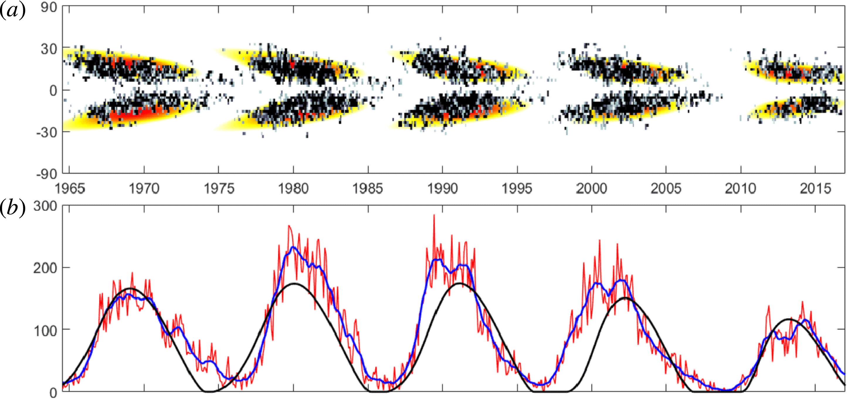
. Comparison of the results using the dynamo model and observations are shown in figure 1. In figure 1(a) we show the butterfly diagram of the Wolf number variation rate
 $2\unicode[STIX]{x03C0}\,\sin \unicode[STIX]{x1D703}\,I(t,\unicode[STIX]{x1D703})$
, obtained from the numerical solution of equations of the dynamo model described in § 2. We also compare these results with those obtained from observations. We use the observed Wolf numbers time series (the real monthly observational data known as the monthly mean total sunspot number, red line). The data are available in open access from the World Data Center SILSO, Royal Observatory of Belgium, Brussels. We also show these observational data using a 13 month sliding (or window) averaging of the observed Wolf numbers time series (blue line). In figure 1(b) we show the time evolution of the Wolf numbers based on the dynamo model and observations. The dynamo model reproduces some of the observed features such as the latitude distribution of the active regions.
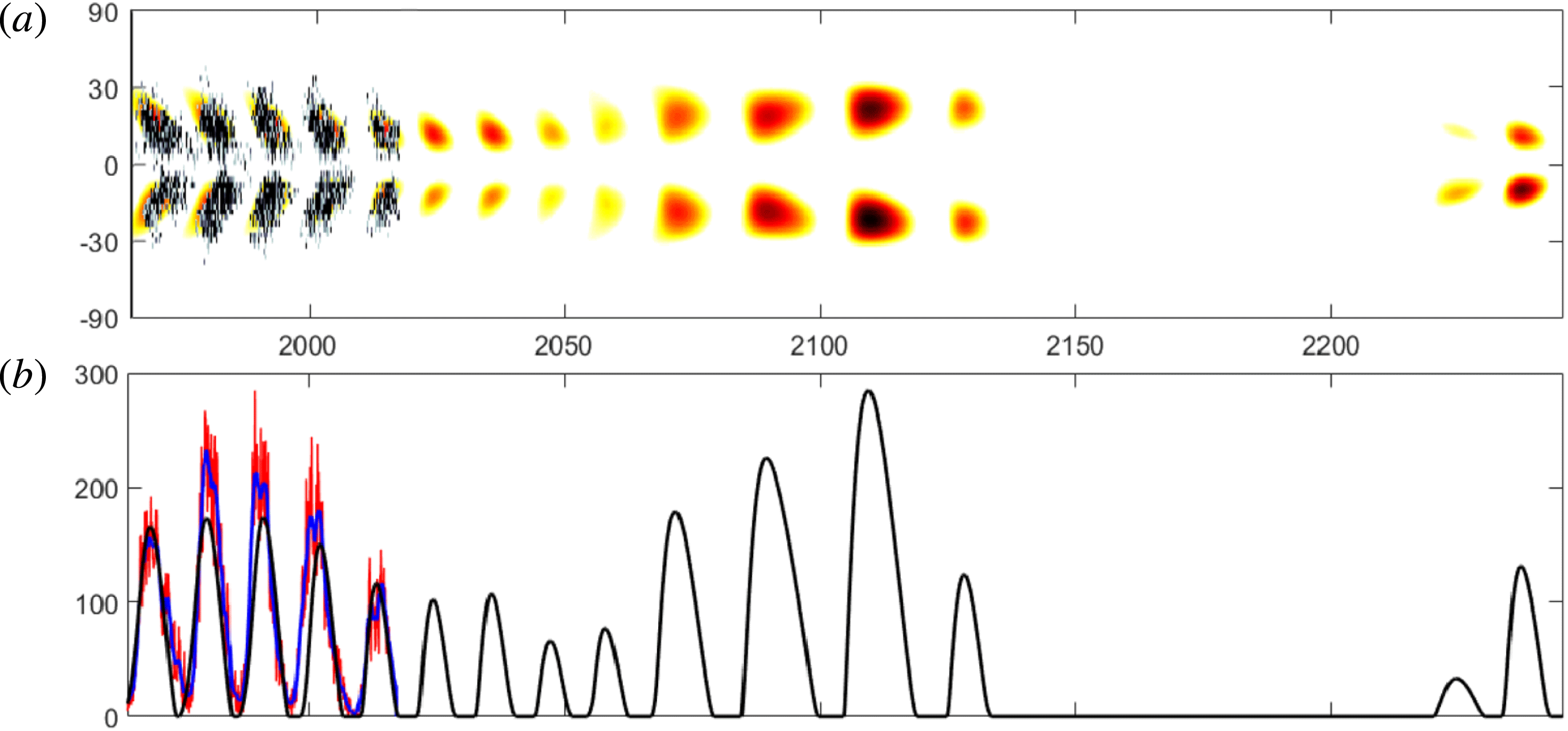
The long-term evolution of these characteristics is shown in figure 2. In particular, the considered dynamo model is able to produce very rich behaviour which includes a decrease of the solar activity during the next half-century up to the minimum (similar to the Dalton minimum), followed by a strong increase of solar activity and the Maunder minimum. The long-term behaviour of the dynamo model (see figure 2 which shows an example of the behaviour of the dynamo model) is not yet a forecast of solar activity, because no observational data have been assimilated into the model here. Note that the simulation discussed here includes 150 years (14 cycles) of transient period. The solutions in figures 1 and 2 are shown at later simulated time, so any transient is not seen in these figures.
Comparison of the results using the dynamo model and observations; (a) butterfly diagram of the Wolf number variation rate
 $2\unicode[STIX]{x03C0}\sin \unicode[STIX]{x1D703}I(t,\unicode[STIX]{x1D703})$
, the dynamo model (colour) and the real monthly observational data (black); (b) the evolution of the Wolf numbers, the dynamo model (black), real observational data (red), and observational data averaged over 13 months (blue).

The poleward propagation of the Wolf numbers is observed in figure 2(a) starting from
 $t=2075$
up to
 $t=2125$
. In the framework of the used simplified dynamo model there is either equatorward propagation of the sunspot belt or poleward propagation of the sunspot belt depending on the level of the magnetic part of the
 $\unicode[STIX]{x1D6FC}$
effect. However, there are no simultaneously coexisting two branches of the dynamo waves. To obtain simultaneously coexisting two branches of the dynamo waves, a two-layer dynamo model with different signs of the differential rotation can be considered in the dynamo model (Belvedere, Kuzanyan & Sokoloff Reference Belvedere, Kuzanyan and Sokoloff2000).
Note that sequences of several cycles with equally high correlation to the solar activity between 1965 and the present day can be found with various different sets of system parameters or even different time spans within one particular simulation. To reach the high correlation between simulated and observed data, we compared different characteristics in simulated and observed sunspot cycles (see figures 9–11 in Kleeorin et al. (Reference Kleeorin, Safiullin, Kleeorin, Porshnev, Rogachevskii and Sokoloff2016)).
The long-term evolution of large-scale magnetic field and the Wolf number time series; (a) butterfly diagram of the Wolf number variation rate
 $2\unicode[STIX]{x03C0}\sin \unicode[STIX]{x1D703}I(t,\unicode[STIX]{x1D703})$
, the dynamo model (colour) and the real monthly observational data (black); (b) the Wolf numbers, the dynamo model (black), real observational data (red), and observational data averaged over 13 months (blue).

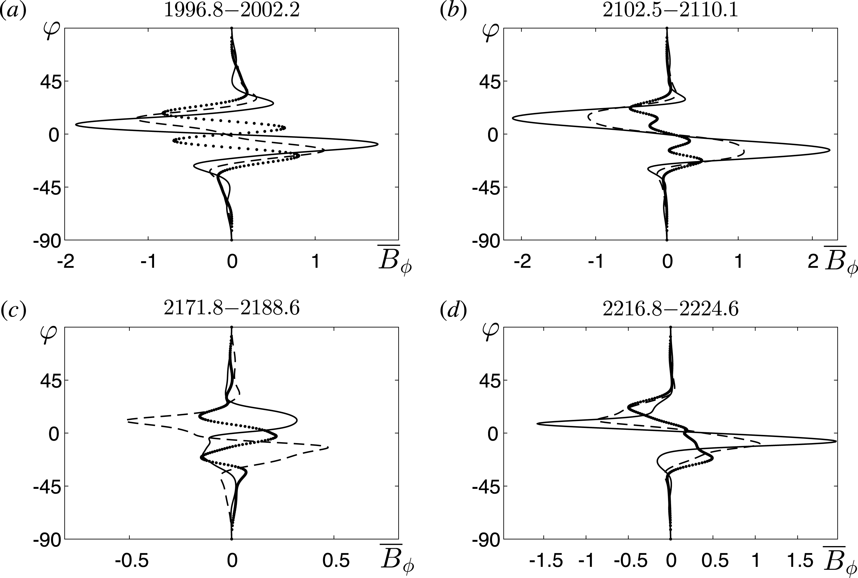
The latitude distribution of the toroidal magnetic field
 $\overline{B}_{\unicode[STIX]{x1D719}}(\unicode[STIX]{x1D711})$
at different stages of magnetic field evolution obtained in the dynamo model: no sunspots (dotted line); beginning of the solar cycle (dashed line) and the maximum of solar activity (solid line). The different panels correspond to different epochs: (a) the modern epoch; (b) the future epoch with high solar activity; (c) the possible Maunder-minimum-like epoch; (d) the epoch after the possible Maunder minimum. The magnetic field is measured in the units of the threshold of the sunspot formation.

In figure 3 we show the latitude distribution of the toroidal magnetic field
 $\overline{B}_{\unicode[STIX]{x1D719}}(\unicode[STIX]{x1D711})$
at different stages of the magnetic field evolution obtained in the framework of the dynamo model described in § 2. This evolution includes lower solar activity without sunspots, the beginning of the new solar cycle and the maximum of solar activity. The different panels correspond to different epochs, e.g. the modern epoch of solar activity; the future epoch with high level of the solar activity; the possible Maunder minimum epoch; and the epoch after the Maunder minimum. The new cycle in the modern epoch starts in high latitudes and the dynamo waves propagates to the equator. On the other hand, in the case of very high level of the solar activity, its maximum reaches very fast at lower latitudes and the dynamo wave propagates to the higher latitudes. During the possible Maunder minimum epoch, a strong asymmetry between the north and the south hemispheres is observed.
After entering into the Maunder minimum the model again comes back on suddenly (see figure 2). Let us discuss what causes the Sun to be kicked into and out of the Maunder minimum. In the considered dynamo model, that includes the equations for the poloidal and toroidal mean magnetic fields, the dynamical equation for the magnetic part of the
 $\unicode[STIX]{x1D6FC}$
effect and the budget equation for the surface density of the Wolf number, can produce rich behaviour including the Maunder minimum. The first three nonlinear equations describe the chaotic behaviour of the large-scale magnetic field. The last equation mimics the sunspots formation which takes into account the threshold for excitation of NEMPI in the large-scale magnetic field. The latter provides switch on and switch off of the sunspot formation (see below).
In figure 2(a) the propagation direction of the dynamo wave changes after which the cycles disappear for almost a century. The physics for the disappearance of the sunspots before starting the Maunder minimum is as follows. When the mean magnetic field decreases below the threshold for the large-scale instability (i.e. NEMPI), the sunspots cannot be formed anymore (see figure 3
c). Before this happened, the level of magnetic activity was high (see figure 2
b), and polar branch of activity dominated (see figure 2
a). The latter is because the total
 $\unicode[STIX]{x1D6FC}$
effect (that determines the direction of the dynamo wave propagation) changes sign. The reason is that when the mean magnetic field becomes strong, the magnetic part of the
 $\unicode[STIX]{x1D6FC}$
effect can be larger than the kinetic part of the
 $\unicode[STIX]{x1D6FC}$
effect, so that the total
 $\unicode[STIX]{x1D6FC}$
changes sign. We note that the magnetic and kinetic parts of the
 $\unicode[STIX]{x1D6FC}$
effect have opposite signs.
We performed a parameter scan using approximately
 $10^{3}$
runs with different sets of parameters to find an optimal set of parameters to reach a high level of correlation between the dynamo model results and observations of the Wolf numbers. Let us discuss how the variations of the parameters affect the results. In our previous study (Kleeorin et al.
Reference Kleeorin, Safiullin, Kleeorin, Porshnev, Rogachevskii and Sokoloff2016) we found that there are two crucial parameters which strongly affect the dynamics of the nonlinear dynamo system: the dynamo number
 $D$
and the initial field
 $B_{\text{init}}^{\text{dip}}$
for the dipole mode, determined by the parameter
 $S_{2}$
. A proper choice of the initial field
 $B_{\text{init}}^{\text{dip}}$
allows us to avoid very long transient regimes to reach the strange attractor. Comparing the results of the dynamo model with observations, we determine the correlation between the numerical simulation data for the Wolf number and the observational data. To find the maximum correlation between the dynamo model results and the observed Wolf numbers, the following parameter scan has been performed:
 $-8800\leqslant D\leqslant -8200$
and
 $0.85\leqslant S_{2}\leqslant 0.95$
(see, e.g. figure 12 in Kleeorin et al. (Reference Kleeorin, Safiullin, Kleeorin, Porshnev, Rogachevskii and Sokoloff2016)). The maximum correlation is obtained when the parameters are
 $D=-8450$
and
 $S_{2}=0.95$
. The function
 $D(\unicode[STIX]{x1D70E})$
determines the region of chaotic behaviour, and for small
 $\unicode[STIX]{x1D70E}$
the dynamo system cannot remain inside the region of the chaotic behaviour. To find the region of the chaotic behaviour, the following parameter scan has been performed:
 $-10^{4}\leqslant D\leqslant -3\times 10^{3}$
and
 $0.3\leqslant \unicode[STIX]{x1D70E}\leqslant 9$
(see, e.g. figure 1 in Kleeorin et al. (Reference Kleeorin, Safiullin, Kleeorin, Porshnev, Rogachevskii and Sokoloff2016)). The parameter
 $\unicode[STIX]{x1D707}$
determines the critical dynamo number,
 $|D_{\text{cr}}|$
, for the excitation of the large-scale dynamo instability. The flux of the magnetic helicity (see (2.8) and (2.9)), characterized by the parameter
 $\unicode[STIX]{x1D705}_{T}$
, cannot be very small to avoid the catastrophic quenching of the
 $\unicode[STIX]{x1D6FC}$
effect. The optimal value for this parameter is
 $\unicode[STIX]{x1D705}_{T}\approx 0.1$
. The variations of the other parameters only weakly affect the obtained results (Kleeorin et al.
Reference Kleeorin, Safiullin, Kleeorin, Porshnev, Rogachevskii and Sokoloff2016).
4 Forecast of solar activity
Any mean-field dynamo model works on a time scale that is larger than 1 year. Indeed, according to the model of solar convective zone by Spruit (Reference Spruit1974), at the bottom of the convective zone, say at depth
 $h_{\ast }\sim 2\times 10^{10}~\text{cm}$
, the magnetic Reynolds number
 $\text{Rm}\sim 2\times 10^{9}$
, the turbulent velocity
 $u_{0}\sim 2\times 10^{3}~\text{cm}~\text{s}^{-1}$
, the turbulent scale
 $\ell _{0}\sim 8\times 10^{9}~\text{cm}$
, so the turn over time of turbulent eddies
 $\ell _{0}/u_{0}\sim 4\times 10^{6}~\text{s}$
(that is 0.13 years). This implies that the mean-field time (the characteristic time of the mean-field variations) should be at least one order of magnitude larger than the turn over time, i.e. approximately 1 year. This refers to a sufficient separation of temporal scales in which case memory effects can be neglected. This implies that a mean-field dynamo model cannot provide the forecast of the solar activity on a time scale of several months. To predict the solar activity on a short time scale, additional methods should be used for the forecast of the solar activity.
To predict solar activity on the time scale of one month we use a method based on a combination of the numerical solution of the nonlinear mean-field dynamo equations and the artificial neural network approach (Fessant et al. Reference Fessant, Pierret and Lantos1996; Conway Reference Conway1998; Hagan et al. Reference Hagan, Demuth and Beale2016). A simplified version of the artificial neural networks method to forecast the solar activity has been used before (Fessant et al. Reference Fessant, Pierret and Lantos1996; Conway Reference Conway1998). However, this method has not been combined with the advanced mean-field approach based on the nonlinear dynamo models, and the used network scheme has not been stable, resulting in a systematic increase of errors. The recent developments in the field of artificial neural networks and the increased computational capabilities of the computers allow us to combine the simulations of the nonlinear mean-field dynamo model with the artificial neural network forecast scheme.
To apply this approach, we use the initial simulations of the Wolf numbers
 $W_{i}^{\text{model}}$
, based on the dynamo model described in § 2, as the basis for the forecast and as the exogenous input in the neural network scheme. Another input are the data
 $W_{i}^{\text{obs}}$
obtained from observations. To perform the forecast
 $W_{i}^{\text{forecast}}$
for the next half a year or longer, we adopt an autoregressive scheme with unknown coefficients (determined during the learning procedure):
 $$\begin{eqnarray}\displaystyle W_{i}^{\text{forecast}}=f_{\text{out}}(\boldsymbol{K}\boldsymbol{w}+\boldsymbol{c}), & & \displaystyle\end{eqnarray}$$
where
 $f_{\text{out}}(x)$
is a linear function of an outer layer of neurons,
 $\boldsymbol{c}$
is the bias vector;
 $\boldsymbol{K}$
is the weight matrix of neurons;
 $\boldsymbol{w}$
is the inputs vector, containing observations
 $W_{i}^{\text{obs}}$
and model estimations
 $W_{i}^{\text{model}}$
. To estimate the weight matrix
 $\boldsymbol{K}$
one needs to minimize the error between the deviations of the forecast data
 $W_{i}^{\text{forecast}}$
from the observational data
 $W_{i}^{\text{obs}}$
.
Equation (4.1) describes a simple ‘one-layer artificial neural network’. However, for our task it is required to use a more complex scheme, e.g. a ‘two-layer artificial neural network’ type of a recurrent dynamic nonlinear autoregressive network, with feedback connections enclosing two layers of the network, defined by the following equation:
 $$\begin{eqnarray}\displaystyle W_{i}^{\text{forecast}}=f_{\text{out}}[\boldsymbol{K}_{2}f_{\text{hidden}}(\boldsymbol{K}_{1}\boldsymbol{w}+\boldsymbol{c}_{1})+\boldsymbol{c}_{2}], & & \displaystyle\end{eqnarray}$$
where
 $f_{\text{hidden}}(x)=[1+\exp (-x)]^{-1}$
is a function of a hidden layer of neurons,
 $\boldsymbol{K}_{1}$
is the weight matrix
 $24\times 8$
of hidden layer neurons,
 $\boldsymbol{K}_{2}$
is the weight matrix
 $1\times 24$
of outer layer neurons,
 $\boldsymbol{c}_{1}$
and
 $\boldsymbol{c}_{2}$
are the corresponding bias vectors,
 $\boldsymbol{w}$
is the input vector
 $8\times 1$
consisting of 4 prior observations
 $W_{i-1}^{\text{obs}},\ldots ,W_{i-4}^{\text{obs}}$
and 4 corresponding model estimations
 $W_{i-1}^{\text{model}},\ldots ,W_{i-4}^{\text{model}}$
.
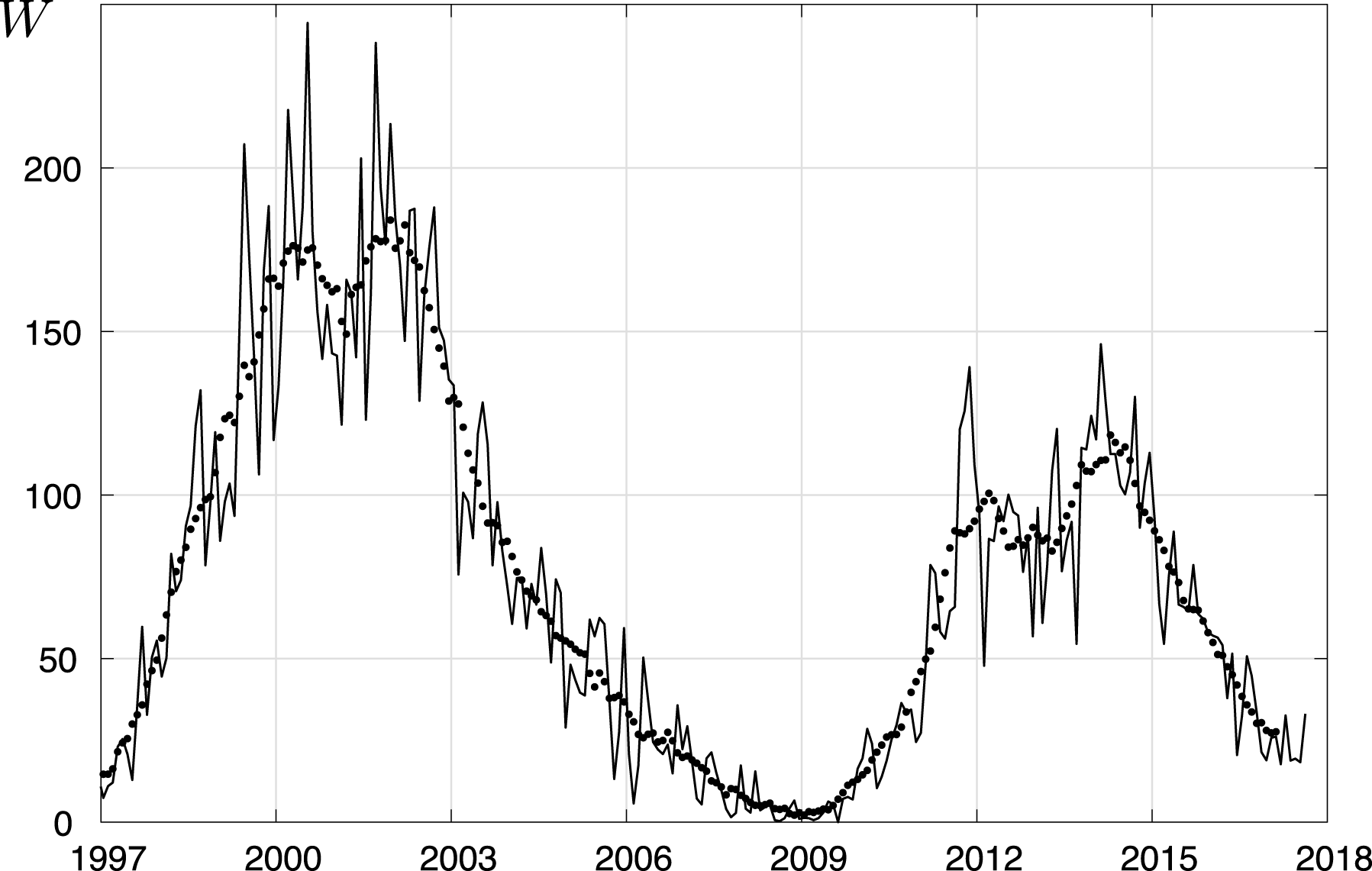
Comparison of the results of the one month forecast of the solar activity (filled circles) with the observed Wolf numbers (solid line).

Equation (4.2) provides a more stable, complex, adaptable and adjustable forecast than (4.1), e.g. in the presence of noise. The learning procedure by Bayesian regularization back propagation has been based on the data of the Wolf numbers from 19–20 cycles, while 21 cycle has been used for the validation process. The input data of the Wolf numbers for the neural network consist of two parts: the prior real observations (e.g. red line in figure 1) and the dynamo model estimations at the same instant (e.g. solid line in figure 1). The output of this neural network is the forecasted monthly Wolf number. Note that we do not use the artificial neural network for any type of optimization or parameter estimation for the initial model. We have already done this in our previous study (Kleeorin et al. Reference Kleeorin, Safiullin, Kleeorin, Porshnev, Rogachevskii and Sokoloff2016). During the learning procedure in the artificial neural network, we minimize the error between the forecast and actual observations not at every instant separately, but over the whole cycle. We stress that the model output yields an initial forecast, i.e. a basis for the final forecast. The artificial neural network serves here as a forecast correction scheme for the simulated sunspots. The correction is done by means of observational data and the model outputs.
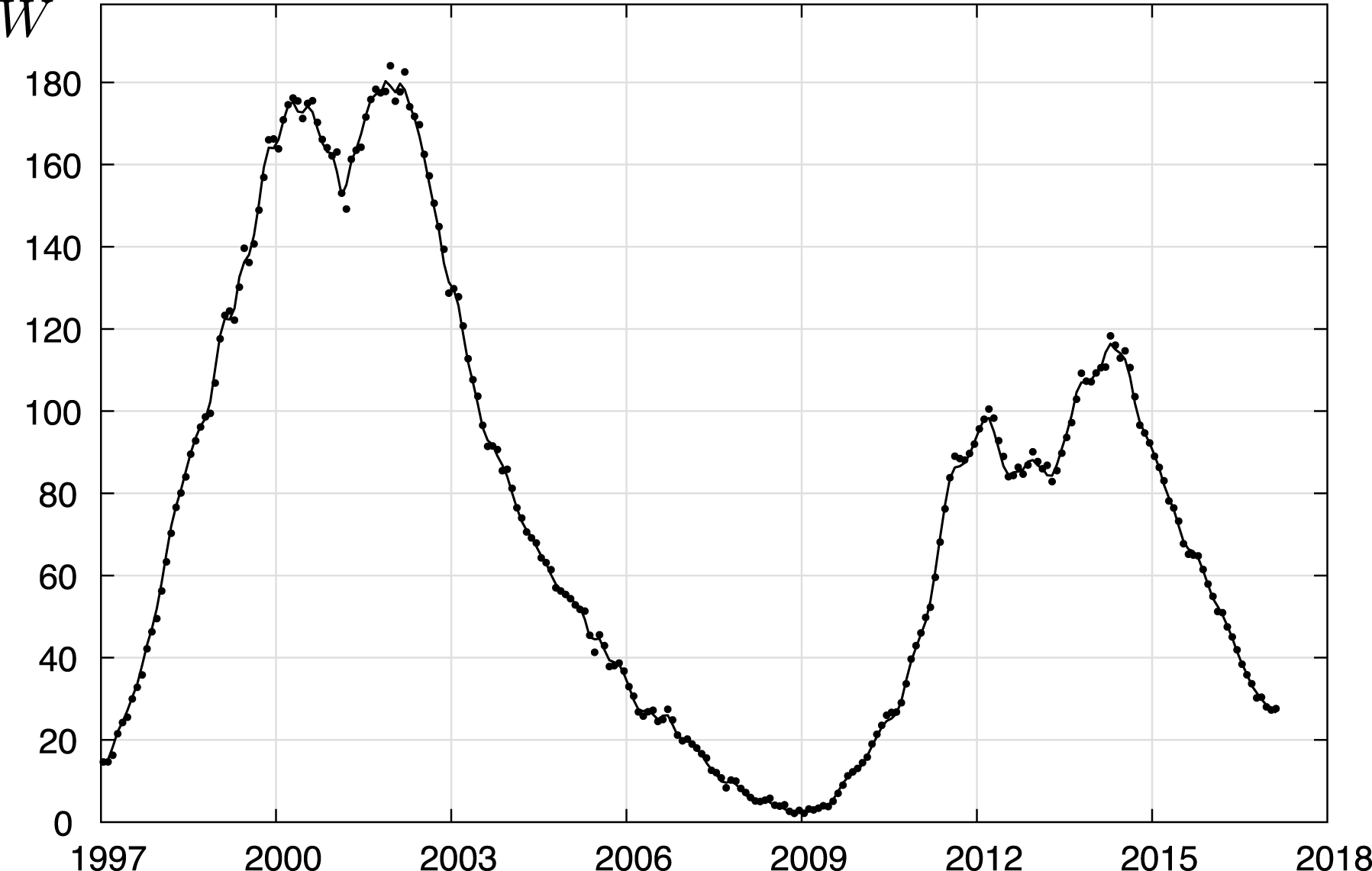
Comparison of the results of the one month forecast of the solar activity (filled circles) with the observed Wolf numbers averaged over 13 month (solid line).

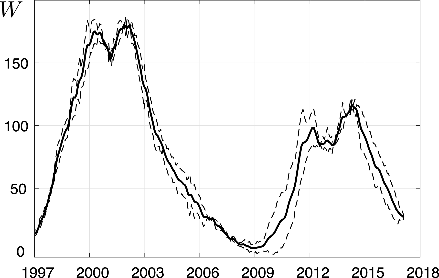
The confidence interval (dashed lines) of the one month forecast of the solar activity compared with the observed Wolf numbers averaged over 13 month (solid line).

The obtained results for the forecast of the solar activity are presented below. In figure 4 we show a comparison of the results of the one month forecast of the solar activity based on the described method with the observed Wolf numbers, while in figure 5 we show the same comparison but with the data of the observed Wolf numbers averaged over 13 month. The sliding (or window) averaging of the observed Wolf number time series has been used here. In figure 4 we use the observed Wolf number time series with 1 month averaging time, while in figure 5 we use the observed Wolf number time series with 13 month averaging time. Sampling time is exactly one month in both cases. For the latter case we show in figure 6 also the confidence interval for this forecast. Note that for the cycle with a higher activity the thickness of the confidence interval is less. The decrease of the confidence interval is also observed in the phase of increasing solar activity (see figure 6). These figures demonstrate a good agreement between the forecast and observation of the solar activity.
We would like to stress that only the combination of the numerical solution of the nonlinear mean-field dynamo equations and the neural network yields good agreement between the forecast and observation. Using only the neural network without the mean-field solution provides reasonable agreement just for 5 years because there is no a long-term memory in the magnetic field evolution.
5 Conclusions
To predict the solar activity, we apply the nonlinear mean-field dynamo model with algebraic and dynamic nonlinearities of the
 $\unicode[STIX]{x1D6FC}$
effect and with a budget equation for the dynamics of Wolf numbers. We use a simplified axisymmetric dynamo model that allows us to obtain very long time series of Wolf number. This dynamo model demonstrates very rich behaviour, reproducing the observed evolution of the magnetic activity during past three centuries. We forecast the solar activity on the time scale of one month adopting a method consisting of a combination of the numerical solution of the nonlinear mean-field dynamo equations and the artificial neural network. A comparison between the forecast of solar activity and the observed Wolf numbers shows a good agreement, which is achieved due to the combined effect of the nonlinear mean-field dynamo model and the artificial neural network technique. Without the mean-field model it is impossible to obtain a reasonable agreement in a long-term evolution.
Acknowledgements
The work of N.S. was supported in part by the Russian Science Foundation (grant no. 18-12-00131). The work of N.K. and I.R. was supported in part by the Research Council of Norway under the FRINATEK (grant no. 231444). N.K. and I.R. would like to acknowledge the hospitality of NORDITA, Ural Federal University and the Kavli Institute for Theoretical Physics in Santa Barbara.