
1. Introduction
Fluid–structure interaction (FSI) problems are of paramount importance in many engineering applications particularly when designing lighter and more robust structures. In particular, the FSI problem in bluff body wakes has been one of the widely studied topics, as it is crucial for the design of many engineering structures, such as bridges, buildings, oil platforms and so on. The flow, which often involves vortex shedding in its wake, causes significant vibration, noise and drag of the given structure through instabilities in fluid and solid motions. Therefore, the understanding of the onset of such instabilities and the resulting self-sustaining drifts/oscillations arising in the FSI problems provides important physical insight into the development of simplified models and control strategies to mitigate the undesirable motions.
Several FSI problems of interest have previously been studied by employing the approaches developed in the context of hydrodynamic stability. Cossu & Morino (Reference Cossu and Morino2000), perhaps one of the earliest works in this field, performed a global linear stability analysis for a spring-mounted circular cylinder allowing for cross-flow oscillations. A similar FSI problem, including the in-line oscillation case, was studied by Meliga & Chomaz (Reference Meliga and Chomaz2014) by coupling the fluid and solid motions via a weakly nonlinear analysis. A linear stability analysis and a nonlinear simulation were also recently performed in Dolci & Carmo (Reference Dolci and Carmo2018) for a spring-mounted circular cylinder with transverse oscillation. More recently, Negi, Hanifi & Henningson (Reference Negi, Hanifi and Henningson2019) investigated a more general global stability analysis framework for FSI problems by employing the arbitrary Lagrangian–Eulerian (ALE) framework (Fernandez & Tallec Reference Fernandez and Tallec2002), while a more detailed and generalized application of the ALE framework can be found in Pfister (Reference Pfister2019) and Pfister & Marquet (Reference Pfister and Marquet2020) where nonlinear numerical simulation and linear stability analysis were also performed for a flow over a circular cylinder with a flexible appendage.
Of particular interest to the present study are flow-induced instabilities, which have previously been observed in a circular cylinder with a rigid or flexible splitter plate attached at the base (Assi, Bearman & Kitney Reference Assi, Bearman and Kitney2009; Assi, Franco & Vestri Reference Assi, Franco and Vestri2014b). The cylinder wake is one of the simplest model problems widely employed to study the onset of vortex shedding, the related FSI problem and their control. It is also directly relevant to industrial applications for the tall building design and the offshore energy harvesting (e.g. drilling rig), to which the addition of a passive appendage may be useful to suppress the vortex shedding. In the case of a rigid bluff body, many previous studies have demonstrated that placing such a device suppresses vortex shedding in the wake of the bluff body (Roshko Reference Roshko1954; Kwon & Choi Reference Kwon and Choi1996; Anderson & Szewczyk Reference Anderson and Szewczyk1997; Ozono Reference Ozono1999; Choi, Jeon & Kim Reference Choi, Jeon and Kim2008). When the appendage is allowed to rotate or deform by imposing a relevant structural dynamics (e.g. coupling through a spring-mass-damper system, elastic motion of the appendage, etc), the cylinder exhibits a flow-induced ‘static’ instability which breaks the symmetry of the flow posed by the cylinder geometry (Cimbala & Garg Reference Cimbala and Garg1991; Assi et al. Reference Assi, Bearman, Kitney and Tognarelli2010; Bagheri, Mazzino & Bottaro Reference Bagheri, Mazzino and Bottaro2012; Assi, Bearman & Tognarelli Reference Assi, Bearman and Tognarelli2014a; Lacis et al. Reference Lacis, Brosse, Ingremeau, Mazzino, Lundell, Kellay and Bagheri2014; Pfister & Marquet Reference Pfister and Marquet2020). It has been proposed that this instability provides an aiding mechanism for flight motion of insects and locomotion of swimming animals (Park et al. Reference Park, Bae, Lee, Jeon and Choi2010; Bagheri et al. Reference Bagheri, Mazzino and Bottaro2012; Lacis et al. Reference Lacis, Brosse, Ingremeau, Mazzino, Lundell, Kellay and Bagheri2014). Further to this, in general, it is also possible to have a FSI-induced ‘dynamic’ or ‘oscillatory’ instability of the body. In relation to this, Pfister & Marquet (Reference Pfister and Marquet2020) recently reported that such an instability appears in a flow over a cylinder attached with a ‘flexible’ plate.
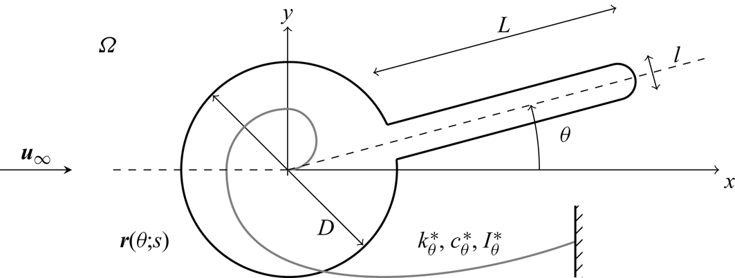
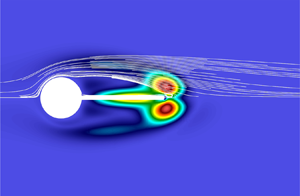
The objective of the present study is to explore the physical origin and the sensitivity of the instabilities discussed above. For this purpose, we consider a circular cylinder with a rigid appendage, as is sketched in figure 1. The rigid body is only allowed to rotate by coupling with a ‘torsional’ spring-mass-damper system in the  $x$–
 $y$ plane, and any three-dimensional rigid body motion and/or deformation are not considered (e.g. streamwise/wall-normal rotation of the cylinder). A global linear instability analysis (Huerre & Monkewitz Reference Huerre and Monkewitz1990; Chomaz Reference Chomaz2005; Theofilis Reference Theofilis2011) is first formulated with introduction of a small perturbation, which allows us to utilise the framework of a stationary cylinder (i.e. the Eulerian framework), while being carefully validated with full nonlinear simulation (Serson, Meneghini & Sherwin Reference Serson, Meneghini and Sherwin2016). Three different types of instabilities (i.e. vortex shedding mode, stationary symmetry breaking mode, oscillatory FSI mode) are found in the context of the global linear instability, and the physical mechanisms on their origin are analysed in detail. In particular, our analysis reveals that the oscillatory FSI instability shares the same origin with the ‘flapping’ mode previously observed in flags and/or flexible plates (Shelley & Zhang Reference Shelley and Zhang2011). The adjoint sensitivity analysis (Giannetti & Luchini Reference Giannetti and Luchini2007; Luchini & Bottaro Reference Luchini and Bottaro2014) is also performed for the first time for the FSI instabilities. Importantly, it is found that the flow around the tip of the appendage plays a crucial role in the generation of the stationary symmetry breaking and the dynamic flapping instabilities, opening a possibility of controlling them with simple redesign of the tip shape.
A schematic diagram of flow and structure configuration. Here,  $\boldsymbol {u}_\infty (=(U_\infty ,0))$ is the free-stream velocity,
 $\theta$ the counter-clockwise rotation angle of the cylinder,
 $k_\theta$ rotational stiffness and
 $c_\theta$ rotational damping coefficient.

This paper is organised as follows. In § 2 the global stability and sensitivity analyses are formulated, and the numerical methods are introduced. The formulated analyses are subsequently applied to the flow-induced instabilities, and the discussion on the role of the flow is given in § 3. This paper concludes in § 4 with some remarks.
2. Problem formulation
We consider a two-dimensional flow over a circular cylinder with a rigid splitter plate, as sketched in figure 1. The free-stream velocity in the streamwise direction is given by  $\boldsymbol {u}_\infty (=(U_\infty ,0))$, and the density and the kinematic viscosity of the fluid are by
 $\rho$ and
 $\nu$, respectively. The diameter of the cylinder is set to be
 $D$, and the length of the splitter plate from the base is given by
 $L$ with the thickness
 $l$. The downstream edge of the splitter plate is also set to be rounded with the radius of
 $l/2$. The cylinder is allowed to rotate about its centre, and the rotational motion is coupled through a torsional spring-mass-damper system. The rotational stiffness, the damping coefficient and the moment of inertia are given by
 $k_\theta ^*$,
 $c_\theta ^*$ and
 $I_\theta ^*$, respectively.
2.1. Equations of motion
The equations of motion and all the related variables (including  $k_\theta ^*$,
 $c_\theta ^*$ and
 $I_\theta ^*$) are made dimensionless with
 $U_\infty$ and
 $D$. The dimensionless spatial location is denoted by
 $\boldsymbol {x}=(x,y)$, where
 $x$ and
 $y$ are the streamwise and transverse coordinates, and the velocity is given by
 $\boldsymbol {u}=(u,v)$ with its streamwise and transverse components
 $u$ and
 $v$. The fluid domain is denoted by
 $\varOmega$, the inner boundary of which is given by the cylinder surface. The centre of the cylinder is set to be located at
 $(x,y)=(0,0)$. When the cylinder is set not to rotate (i.e. reference position), the surface location of the cylinder forms a set defined by
 \begin{equation} \partial \varOmega_s = \left\{(x,y) \,|\,(x,y) = (r(s)\cos(s), r(s)\sin(s))\ \mathrm{where}\ s \in [0, 2{\rm \pi}) \right\}, \end{equation}
where  $s$ is the parameter of the curve
 $\partial \varOmega _s$, physically equivalent to the azimuthal angle, and
 $r(s)$ is the radial location of the cylinder surface. If
 $\boldsymbol {r}_0(s)$ is set to be a point on the cylinder surface (i.e.
 $\boldsymbol {r}_0(s)\in \partial \varOmega _s$), it is written as
 \begin{equation} \boldsymbol{r}(\theta;s) = \boldsymbol{R}(\theta) \boldsymbol{r}_0(s) \end{equation}
for a non-zero rotation angle  $\theta$, where
 $\boldsymbol {R}(\theta )$ is the rotation matrix
 \begin{equation} \boldsymbol{R}(\theta) = \begin{bmatrix} \cos \theta & -\sin \theta \\ \sin \theta & \cos \theta \end{bmatrix}. \end{equation}
The equations for fluid motion are given by the following momentum and mass conservation laws:
 $$\begin{gather} \frac{\partial \boldsymbol{u} }{\partial t } + \left(\boldsymbol{u} \boldsymbol{\cdot} \boldsymbol{\nabla}\right)\boldsymbol{u} ={-}\boldsymbol{\nabla} p + \frac{1}{Re}\nabla^{2}\boldsymbol{u}, \end{gather}$$
 $$\begin{gather}\boldsymbol{\nabla}\boldsymbol{\cdot} \boldsymbol{u} =0. \end{gather}$$
Here  $p$ is the dimensionless pressure and
 $Re = {U}_{\infty }D/\nu$ is the Reynolds number. The boundary condition at the cylinder surface is given by
 \begin{equation} \boldsymbol{u}(\boldsymbol{r}(\theta;s))=\frac{\text{d} \boldsymbol{r}(\theta;s)}{\text{d}t}. \end{equation}
For the rotational motion of the cylinder, the following equation is based on a linear spring-mass-damper system:
 \begin{equation} \ddot \theta + \frac{4 {\rm \pi}\zeta_\theta }{U_R } \dot \theta+ \left( \frac{2 {\rm \pi}}{U_R} \right)^2 \theta = \frac{ 4{m}_z(\boldsymbol{u},p)}{{\rm \pi} I_{\theta,r}}. \end{equation}
Here  $\dot {(\cdot )}$ indicates
 $\text {d}/\text {d}t$, and
 $I_{\theta ,r}$,
 $\zeta _\theta$ and
 $U_R$ are the dimensionless reduced moment of inertia, damping ratio and reduced velocity, i.e.
 \begin{equation} I_{\theta,r} = \frac{4 I_\theta}{\rm \pi},\quad \zeta_\theta = \frac{c_\theta}{2\sqrt{k_\theta I_\theta}} \quad \text{and} \quad U_R = \frac{2{\rm \pi}}{\omega_n} \end{equation}
with the dimensionless natural frequency 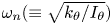 $\omega _n(\equiv \sqrt {k_\theta /I_\theta })$, and the dimensionless moment of inertia, damping coefficient and rotational stiffness (or spring constant),
 $I_\theta$,
 $c_\theta$ and
 $k_\theta$, respectively. Lastly,
 $m_z$ is the moment applied to the cylinder by fluid force per unit span,
 \begin{equation} m_z(\boldsymbol{u},p) \boldsymbol{k} = \oint _{ \partial \varOmega_s }{ \left\{ \boldsymbol{r} \times \left( \boldsymbol{\sigma} \boldsymbol{\cdot} \boldsymbol{n} \right)\right\}}\text{d}l, \end{equation}
where  $\boldsymbol {k}$ is the unit vector along the
 $z$ direction orthogonal to the
 $x$–
 $y$ plane,
 $\boldsymbol {n}$ is the outward unit normal vector on
 $\partial \varOmega _s$ with
 $\boldsymbol {n}(\theta ;s)=\boldsymbol {R}(\theta )\boldsymbol {n}_0(s)$ with
 $\boldsymbol {n}_0(s)=\boldsymbol {n}(0;s)$, and
 \begin{equation} \boldsymbol{\sigma}={-}p\boldsymbol{I}+Re^{{-}1} \left[\boldsymbol{\nabla} \boldsymbol{u}+ \left(\boldsymbol{\nabla} \boldsymbol{u}\right)^\textrm{T} \right], \end{equation}
where  $\boldsymbol {I}$ is the identity operator in
 $\mathbb {R}^{2 \times 2}$.
2.2. Linear stability
We first consider the steady basic state of (2.3) and (2.4). It is evident that the base flow  $\boldsymbol {u}_0$ (i.e. basic state for fluid motion) is steady and symmetric about
 $y=0$, and is obtained by the steady solution to (2.3) with the boundary condition
 $\boldsymbol {u}_0(\boldsymbol {r}_0(s))=\boldsymbol {0}$. The symmetric base flow also yields
 $m_z(\boldsymbol {u}_0,p_0)=0$, resulting in the stationary basic state for solid motion given by
 $\theta _0=0$. The linear stability of the basic state is subsequently examined by introducing a small perturbation to both fluid and solid motions with
 $\epsilon _1 \ll 1$, i.e.
 \begin{equation} \boldsymbol{u} = \boldsymbol{u}_0 + \epsilon_1 \boldsymbol{u}',\quad p = p_0 + \epsilon_1 p', \quad \theta = \theta_0 + \epsilon_1 \theta',\quad \boldsymbol{r} = \boldsymbol{r}_0 + \epsilon_1 \boldsymbol{r}',\quad \boldsymbol{n} = \boldsymbol{n}_0 + \epsilon_1 \boldsymbol{n}'. \end{equation}
The linearised equations of fluid motion at  $O(\epsilon _1)$ are given by
 $$\begin{gather} \frac{\partial \boldsymbol{u}' }{\partial t } + (\boldsymbol{u}'\boldsymbol{\cdot}\boldsymbol{\nabla}) \boldsymbol{u}_0 + (\boldsymbol{u}_0 \boldsymbol{\cdot}\boldsymbol{\nabla})\boldsymbol{u}' ={-}\boldsymbol{\nabla} p' + Re^{{-}1} \nabla^{2}\boldsymbol{u}', \end{gather}$$
 $$\begin{gather}\boldsymbol{\nabla}\boldsymbol{\cdot} \boldsymbol{u}' =0. \end{gather}$$
Using (2.2), (2.3c) and (2.5a–e), the boundary condition for  $\boldsymbol {u}'$ is obtained such that
 \begin{equation} \boldsymbol{u}'(\boldsymbol{r}_0(s))=\boldsymbol{r}_1(s)\dot \theta'-(\boldsymbol{\nabla}\boldsymbol{u}_0 \boldsymbol{\cdot}\boldsymbol{r}_1(s))\theta', \end{equation}
where  $\boldsymbol {r}_1(s)=\boldsymbol {r}'(s)/\theta '$ and
 \begin{equation} \boldsymbol{r}_1(s) = \underbrace{\left.\frac{\text{d}\boldsymbol{R}(\theta)}{\text{d}\theta}\right|_{\theta= \theta_0}}_{{\equiv} \boldsymbol{R}_1} \boldsymbol{r}_0(s) \quad \text{with}\ \boldsymbol{R}_1=\begin{bmatrix} 0 & -1 \\ 1 & 0 \end{bmatrix}. \end{equation}
The linearised equations of solid motion are given by
 \begin{equation} \ddot \theta' + \frac{4 {\rm \pi}\zeta_\theta }{U_R } \dot \theta'+ \left( \frac{2 {\rm \pi}}{U_R} \right)^2 \theta' = \frac{ 4{m}_z'}{{\rm \pi} I_{\theta,r}}, \end{equation}
where
 \begin{align} {m}_z' &= \oint _{ \partial \varOmega_s }{ \left[ \boldsymbol{r}' \times \left( \boldsymbol{\sigma}_0 \boldsymbol{\cdot} \boldsymbol{n}_0 \right) + \boldsymbol{r}_0 \times \left( (\boldsymbol{\sigma}' +\boldsymbol{\sigma}_b)\boldsymbol{\cdot} \boldsymbol{n}_0 \right) + \boldsymbol{r}_0 \times \left( \boldsymbol{\sigma}_0 \boldsymbol{\cdot} \boldsymbol{n}' \right)\right]}\text{d}l \nonumber\\ &= \oint _{ \partial \varOmega_s }{ \left[ \boldsymbol{r}_0 \times \left(\boldsymbol{(\boldsymbol{\sigma}}' +\boldsymbol{\sigma}_{b}+\boldsymbol{\sigma}_{g}) \boldsymbol{\cdot} \boldsymbol{n}_0 \right) \right] }\text{d}l, \end{align}
with the contribution from the first-order quantities
 \begin{equation} \boldsymbol{\sigma}'={-}p'\boldsymbol{I}+Re^{{-}1} \left[ \boldsymbol{\nabla} \boldsymbol{u}'+ \left( \boldsymbol{\nabla} \boldsymbol{u}'\right)^\textrm{T} \right], \end{equation}
the stress contribution of base flow to the changed geometry
 \begin{equation} \boldsymbol{\sigma}_{b}=\begin{bmatrix} \boldsymbol{\nabla}\boldsymbol{ \sigma}_{0,xx} \boldsymbol{\cdot} \boldsymbol{r}_1(s) & \boldsymbol{\nabla}\boldsymbol{ \sigma}_{0,xy} \boldsymbol{\cdot} \boldsymbol{r}_1(s) \\ \boldsymbol{\nabla}\boldsymbol{ \sigma}_{0,yx} \boldsymbol{\cdot} \boldsymbol{r}_1(s) & \boldsymbol{\nabla}\boldsymbol{ \sigma}_{0,yy} \boldsymbol{\cdot} \boldsymbol{r}_1(s) \end{bmatrix}\theta', \end{equation}
and the one of the geometrical change (i.e.  $\boldsymbol {r}'$ and
 $\boldsymbol {n}'$)
 \begin{equation} \boldsymbol{\sigma}_{g}=\left[\boldsymbol{R}_1^\textrm{T} \boldsymbol{\sigma}_{0}+ \boldsymbol{\sigma}_{0} \boldsymbol{R}_1\right]\theta', \end{equation}
where  $\sigma _g$ is obtained using (2.6d) and
 $\boldsymbol {n}'(s)=[\boldsymbol {R}_1\boldsymbol {n}_0(s)]\theta '$. We note that
 $\sigma _b$ and
 $\sigma _g$ represent the effective stiffness originating from the base flow stress and the geometrical change by the rotation of the cylinder. It has recently been shown that their contribution is analytically zero only for rigid body motions (Negi et al. Reference Negi, Hanifi and Henningson2019), and we have made the same observation numerically in the present study. Therefore, we shall not consider the contribution of these terms (i.e.
 $\sigma _b$ and
 $\sigma _g$) to
 $m_z'$.
Now, we consider a normal-mode solution to the system of (2.6) and (2.7),
 \begin{equation} \boldsymbol{u}'(x,y,t)=\hat{\boldsymbol{u}}(x,y)\,\textrm{e}^{\lambda t},\quad p'(x,y,t)=\hat{p}(x,y)\,\textrm{e}^{\lambda t}, \quad \theta'{(t)}=\hat{\theta}\,\textrm{e}^{\lambda t},\quad \phi'{(t)}=\hat{\phi}\,\textrm{e}^{\lambda t}, \end{equation}
where  $\phi '= \dot \theta '$ and
 $\lambda$ is a complex eigenvalue to be obtained. By defining a state variable
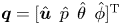 $\boldsymbol {q}=[\hat {\boldsymbol {u}}\enspace \hat {p}\enspace \hat {\theta }\enspace \hat {\phi }]^\textrm {T}$, the following eigenvalue problem for global linear stability is obtained:
 \begin{equation} \lambda \boldsymbol{M}\boldsymbol{q}=\boldsymbol{L}\boldsymbol{q}. \end{equation}
Here
 \begin{equation} \boldsymbol{M}=\left[\begin{array}{cccc} \boldsymbol{I} & 0 & 0 & 0 \\ 0 & 0 & 0 & 0 \\ 0 & 0 & 1 & 0 \\ 0 & 0 & 0 & 1 \end{array}\right], \quad \boldsymbol{L}=\left[\begin{array}{cccc} \boldsymbol{N} & -\boldsymbol{\nabla} & 0 & 0 \\ \boldsymbol{\nabla}\boldsymbol{\cdot} & 0 & 0 & 0 \\ 0 & 0 & 0 & 1 \\ m_{z,\nu}' & m_{z,p}' & -(2{\rm \pi}/U_R)^2 & -4{\rm \pi} \zeta_\theta/U_R \end{array}\right], \end{equation}
and
 \begin{equation} \boldsymbol{N}\hat{\boldsymbol{u}}={-}(\hat{\boldsymbol{u}}\boldsymbol{\cdot}\boldsymbol{\nabla}) \boldsymbol{u}_0 - (\boldsymbol{u}_0 \boldsymbol{\cdot} \boldsymbol{\nabla})\hat{\boldsymbol{u}}+Re^{{-}1} \nabla^2\hat{\boldsymbol{u}}, \end{equation}
with the boundary condition
 \begin{equation} \hat{\boldsymbol{u}}(\boldsymbol{r}_0(s))=\boldsymbol{r}_1(s) \hat{\phi}-(\boldsymbol{\nabla}\boldsymbol{u}_0 \boldsymbol{\cdot} \boldsymbol{r}_1(s))\hat{\theta}, \end{equation}
and
 $$\begin{gather} m_{z,\nu}' \hat{\boldsymbol{u}} = \frac{1}{Re}\oint_{\partial \varOmega_s }{\left[ \boldsymbol{r}_0 \times \left(\left[\boldsymbol{\nabla} \hat{\boldsymbol{u}}+\left(\boldsymbol{\nabla}\hat{\boldsymbol{u}}\right)^\textrm{T}\right] \boldsymbol{\cdot} \boldsymbol{n}_0\right)\right] \boldsymbol{\cdot} \boldsymbol{k}}\text{d}l, \end{gather}$$
 $$\begin{gather}m_{z,p}' \hat{p} ={-}\oint_{\partial \varOmega_s }{\left[\boldsymbol{r}_0 \times \left(\hat{p}\boldsymbol{I} \boldsymbol{\cdot} \boldsymbol{n}_0 \right) \right]\boldsymbol{\cdot} \boldsymbol{k}}\text{d}l. \end{gather}$$
Here, we note that (2.9) is a two-way coupled system between fluid and structural motions: the effect of fluid motion to structural dynamics is coupled with the  $m_{z,\nu }'$ and
 $m_{z,p}'$ in
 $\boldsymbol {L}$, while that of structural motion to fluid flow is depicted by the boundary condition (2.9d).
2.3. Adjoint sensitivity analysis
Let us consider a small perturbation given to the linear operator of the eigenvalue problem in (2.9), i.e.  $\boldsymbol {L} \rightarrow \boldsymbol {L}+\epsilon _2 \delta \boldsymbol {L}$ with
 $\epsilon _2 \ll 1$. This then yields small changes in the eigenvalue and the eigenfunction, such that
 \begin{equation} \lambda \rightarrow \lambda+\epsilon_2 \delta\lambda + O(\epsilon_2^2),\quad \boldsymbol{q} \rightarrow\boldsymbol{q}+\epsilon_2 \delta \boldsymbol{q}+O(\epsilon_2^2). \end{equation}
Using the standard method (e.g. Chomaz Reference Chomaz2005; Giannetti & Luchini Reference Giannetti and Luchini2007), the sensitivity of the eigenvalue is obtained as
 \begin{equation} \delta \lambda = \frac{\langle \delta \boldsymbol{L}\boldsymbol{q}, \boldsymbol{q}^{\dagger} \rangle}{\langle \boldsymbol{q}, \boldsymbol{q}^{\dagger} \rangle}. \end{equation}
Here,  $\langle \cdot , \cdot \rangle$ is an inner product defined in Appendix A, and is introduced such that
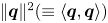 $\|\boldsymbol {q} \|^2(\equiv \langle \boldsymbol {q},\boldsymbol {q} \rangle )$ physically represents the total energy of the given system. Also,
 $\boldsymbol {q}^{\dagger} = [\hat {\boldsymbol {u}}^{\dagger} \enspace \hat {p}^{\dagger} \enspace \hat {\theta }^{\dagger} \enspace \hat {\phi }^{\dagger} ]^\textrm {T}$ is the adjoint state variable, and the corresponding equations are given by
 \begin{equation} \lambda^{\dagger} \boldsymbol{M}\boldsymbol{q}^{\dagger}{=}\boldsymbol{L}^{\dagger}\boldsymbol{q}^{\dagger} \end{equation}
with
 \begin{equation} \boldsymbol{L}^{\dagger}{=}\left[\begin{array}{cccc} \boldsymbol{N}^{\dagger} & \boldsymbol{\nabla} & 0 & 0 \\ \boldsymbol{\nabla}\boldsymbol{\cdot} & 0 & 0 & 0 \\ m_{z,\nu}^{{{\dagger}}} & m_{z,p}^{{{\dagger}}} & 0 & -1 \\ I_\theta^{{-}1} m_{z,\nu}' & I_\theta^{{-}1} m_{z,p}' & (2{\rm \pi}/U_R)^2 & -4{\rm \pi} \zeta_\theta/U_R \end{array}\right], \end{equation}
where
 \begin{equation} \boldsymbol{N}^{\dagger} \hat{\boldsymbol{u}}^{\dagger}{=}(\boldsymbol{u}_0 \boldsymbol{\cdot}\boldsymbol{\nabla}) \hat{\boldsymbol{u}}^{\dagger}{+} \hat{\boldsymbol{u}}^{\dagger} \boldsymbol{\cdot} \left(\boldsymbol{\nabla}\boldsymbol{u}_0 \right)^\textrm{T} +Re^{{-}1} \nabla^2\hat{\boldsymbol{u}}^{\dagger}, \end{equation}
with the boundary condition
 \begin{equation} \hat{\boldsymbol{u}}^{\dagger}(\boldsymbol{r}_0(s))={-}\boldsymbol{r}_1(s) \hat{\phi}^{\dagger}, \end{equation}
and
 $$\begin{gather} m_{z,\nu}^{{{\dagger}}} \hat{\boldsymbol{u}}^{\dagger}{=}{-}\frac{1}{k_\theta Re} \oint_{\partial \varOmega_s}{\left[\left(\boldsymbol{\nabla}\boldsymbol{u}_0 \boldsymbol{\cdot} \boldsymbol{r}_1\right) \boldsymbol{\cdot} \left(\left[\boldsymbol{\nabla} \hat{\boldsymbol{u}}^{\dagger}{+} \left(\boldsymbol{\nabla} \hat{\boldsymbol{u}}^{\dagger} \right)^\textrm{T}\right] \boldsymbol{\cdot} \boldsymbol{n}_0\right)\right]}\text{d}l, \end{gather}$$
 $$\begin{gather}m_{z,p}^{{{\dagger}}} \hat{p}^{\dagger}{=}{-}\frac{1}{k_\theta} \oint _{\partial \varOmega_s}{\left[\left(\boldsymbol{\nabla}\boldsymbol{u}_0 \boldsymbol{\cdot} \boldsymbol{r}_1\right)\boldsymbol{\cdot} \left(\hat{p}^{\dagger} \boldsymbol{I} \boldsymbol{\cdot} \boldsymbol{n}_0\right)\right]}\text{d}l. \end{gather}$$
We note that  $\lambda ^{\dagger}$ is the adjoint eigenvalue given by
 $\lambda ^{\dagger} =\bar {\lambda }$, where the overbar
 $(\bar {\cdot })$ indicates the complex conjugate. Also, the adjoint Navier–Stokes operator in (2.12c) is coupled with the structural adjoint operator through a non-trivial boundary condition (2.12d). In the absence of this boundary condition, (2.12c) is only able to describe the sensitivity of fluid motion to a perturbation in flow field, implying that the boundary condition provides a way for (2.12c) to describe the sensitivity of fluid motion to a perturbation in structural motion. The detailed derivation of the adjoint equations and the boundary conditions are provided in Appendix A.
The sensitivity of the eigenvalue can now be studied with (2.11) by considering various types of the perturbation  $\boldsymbol {\delta L}$ depending on the control mechanism of interest, e.g. secondary cylinder (Strykowski & Sreenivasan Reference Strykowski and Sreenivasan1990; Marquet, Sipp & Jacquin Reference Marquet, Sipp and Jacquin2008). Instead of focusing on a particular perturbation mechanism, here we shall consider a perturbation of a general form given by
 \begin{equation} \delta\boldsymbol{L} = \boldsymbol{M} \boldsymbol{q}. \end{equation}
Here, the perturbation for fluid variables is in the form of a spatially localised feedback identical to that in Giannetti & Luchini (Reference Giannetti and Luchini2007), while that for structural variables lies in the stiffness  $k_\theta$ and
 $I_\theta$ which directly affect the total energy of the fluid–structure system here. In particular, application of the Cauchy–Schwarz inequality to (2.11) for
 $\delta \boldsymbol {L}$ in (2.13) gives the following bound for
 $\delta \lambda$:
 \begin{equation} \left| \delta \lambda \right| \le \frac{\left\| \hat{\boldsymbol{u}} \right\|_F \left\| \hat{\boldsymbol{u}}^{\dagger} \right\|_F+|\hat{\theta}||\hat{\theta}^{\dagger}|+ |\hat{\phi}||\hat{\phi}^{\dagger}|}{ \left| \left\langle \boldsymbol{q}, \boldsymbol{q}^{\dagger} \right\rangle \right|}. \end{equation}
Here  $\| \cdot \|_F^2=\int _\varOmega (\cdot )^2\,\text {d}\kern0.06em \boldsymbol {x}$. Using (2.14), one may define a sensitivity field given in the fluid domain
 $\varOmega$, such that
 \begin{equation} \varTheta_F \left (x,y \right) = \frac{\left\|\hat{\boldsymbol{u}} \right\|_F \left\| \hat{\boldsymbol{u}}^{\dagger} \right\|_F}{ \left| \left\langle \boldsymbol{q}, \boldsymbol{q}^{\dagger} \right\rangle \right|}, \end{equation}
which characterises the spatial location where the given eigenvalue responds sensitively to the fluid part of the perturbation in (2.13). Similarly, a scalar quantity characterising the sensitivity to the solid part of the perturbation can be defined, such that
 \begin{equation} \varTheta_S = \frac{|\hat{\theta}||\hat{\theta}^{\dagger}|+|\hat{\phi}| |\hat{\phi}^{\dagger}|}{\left|\left\langle \boldsymbol{q}, \boldsymbol{q}^{\dagger} \right\rangle \right|}. \end{equation}
Comparison of the values of  $\varTheta _F$ with those of
 $\varTheta _S$ will then allow us to characterise the relative importance of one to the other. Finally, we note that the sensitivity in (2.15) measures the effect of a perturbation in the form of (2.13) in terms of the total energy of the system. Therefore, the coupling effect for the instabilities originating from FSI should be reflected in (2.15). Having pointed this out, the form of (2.13) does not directly add a perturbation to the coupling terms in (2.3c) and (2.4a). However, adding a perturbation to (2.3c) is equivalent to considering a different boundary condition that is not the no-slip condition (e.g. a slip boundary condition), and, similarly, having a physically feasible perturbation to (2.4a) is equivalent to changing
 $I_{\theta ,r}$, which will be examined through a parametric study in § 3.
2.4. Numerical methods
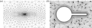
The base flow state as well as the direct and adjoint problems, are solved numerically through a Spectral/hp approach (Cantwell et al. Reference Cantwell2015) available through the open source framework Nektar++, and the domain  $\varOmega$ is discretised and locally refined using Nekmesh, the built-in mesh generator of Nektar++ which generates curvilinear boundary conforming meshes. Quadrilateral elements are adopted in the boundary layer's region close to the structure's interface organised in structured layers and triangular elements are used in the other regions of the domain, resulting in an unstructured mesh. A representative mesh is shown in figure 2 consisting of 1754 elements and 28 104 degrees of freedom.
Example of size distribution of elements (a) used in the mesh for the splitter plate of length  $L/D=1$. The close-up in (b) shows the quadrature points for
 $P=7$.

The fluid equations are solved using a high-order splitting/velocity-correction projection method. This scheme (see Karniadakis, Israeli & Orszag Reference Karniadakis, Israeli and Orszag1991; Guermond & Shen Reference Guermond and Shen2003) consists in first obtaining the pressure field by solving the pressure Poisson equation using boundary conditions derived from the governing equation that enforce the incompressibility condition. Subsequently the velocity field is obtained through a series of Helmholtz equations, arising from the viscous operator in the governing equations, which also enforces the velocity boundary conditions.
The computational domain  $\varOmega$ is symmetric in both the in-flow and cross-flow directions and is chosen such that the origin
 $(x,y)=(0,0)$ is located at the centre of the cylinder for all simulations presented in this study. For the stationary case, different domain sizes have been used to ensure acceptable agreement between forward and adjoint problems while limiting the computational costs (see § B.1), whereas for the rotating cylinder simulations § 3.1, the upstream/downstream dimensions are chosen as
 $-40< x/D<40$ and the cross-flow dimensions as
 $-30< y/D<30$ as it shows excellent agreement comparing direct to adjoint eigenvalues (see § B.2). For all simulations, a polynomial projection basis of order
 $P=7$ and a dimensionless time step of
 $t=10^{-3}$ were adopted. The eigenvalues are then subsequently computed by employing the standard Arnoldi iteration, i.e. the eigenvalue computation approach in the Krylov subspace constructed by the temporal snapshots of the linearised and the adjoint systems. The base flow generation is undertaken by solving (2.3) and (2.4) in the fixed reference position of the cylinder (i.e.
 $\theta =0$), along with a ‘no slip’ boundary condition at the fluid/solid boundary interface. When vortex shedding is not present, the steady base flow is obtained directly through time marching to a steady state. In the regime where vortex shedding is supposed to appear, the base flow can be obtained with the selective frequency damping (SFD) originally proposed by Akervik et al. (Reference Akervik, Brandt, Henningson, Hoepffner, Marxen and Schlatter2006). In the present study, the SFD proposed by Jordi, Cotter & Sherwin (Reference Jordi, Cotter and Sherwin2014) was used.
The stability and sensitivity analyses are carried out by computing leading eigenvalues of the linearised Navier–Stokes and associated adjoint equations with the Arnoldi iteration, as discussed in Barkley, Blackburn & Sherwin (Reference Barkley, Blackburn and Sherwin2008). As formulated in § 2, the cylinder is set to be in the reference position (i.e.  $\theta _0=0$), and its rotational effect is implemented with the blowing/suction boundary conditions in (2.6c) and in (2.12d) at the solid interface. At each time step, the fluid equations are advanced using the velocity-correction scheme described above, and the resulting velocity and pressure fields are used to compute the aerodynamic moments in (2.7) and (2.9). The structural equations are then solved numerically using second-order linear multistep methods, namely the Adams–Bashforth (for the angular velocities) and Adams–Moulton (for the angular positions) schemes. The resulting structural position and velocity are then updated for the boundary conditions at the solid interface. This loosely coupled approach is known to have numerical instabilities at low added mass ratios (Gerbeau, Nobile & Causin Reference Gerbeau, Nobile and Causin2005). To address this issue, we have implemented a fictitious inertia to the structural scheme as described in Baek & Karniadakis (Reference Baek and Karniadakis2012). The linear stability calculation has been verified by comparing with fully nonlinear simulations of the rotating cases. For the fully nonlinear simulations, a coordinate transformation technique proposed by Luo & Bewley (Reference Luo and Bewley2004) is adopted. The details of its application to the velocity-correction scheme approach and the subsequent verification can be found in Serson et al. (Reference Serson, Meneghini and Sherwin2016).
3. Results and discussions
We primarily consider a fixed reduced velocity  $U_R=3937$ (corresponding to
 $I_\theta = 50$,
 $c_\theta = 0$ and
 $k_\theta = 10^{-4}$). The value of such a reduced velocity is chosen as it displays the three instabilities of interest well (i.e. the vortex shedding, the symmetry breaking and the torsional flapping) with reasonable variations of the other parameters. We shall focus on following three questions related to two-dimensional flow past a cylinder with a splitter plate of different lengths.
(i) How does the rotational motion of the cylinder modify the instability of fluid motion (i.e. vortex shedding)?
(ii) What are the instabilities caused by fluid–structure interaction and how do they compare to that arising in the flow past the fixed body case as the length of the splitter plate varies?
(iii) How does the structure of the sensitivity field of these instability modes change with the length of the splitter plate?
To address questions (i) and (ii) above, we first consider the neutral stability curves of the various instability modes. Three types of instability modes were found in the presence of FSI, and their eigenvalues are denoted by  $\lambda ^{SB}$ (symmetry breaking mode denoted by SB),
 $\lambda ^{TF}$ (torsional flapping denoted by TF) and
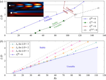
 $\lambda ^{VS}$ (vortex shedding mode denoted by VS), respectively. Figure 3(a) summarises the critical Reynolds numbers for the onset of two leading FSI instability modes in the flow past the rotating cylinder as a function of the splitter plate length. As a reference, the onset of the vortex shedding mode in the absence of any fluid structural interaction is also plotted, and its eigenvalue is denoted by
 $\lambda ^{VS,F}$ (the black dotted line with open square symbols). As the Reynolds number increases, the first instability mode arises for
 $L/D < 3.5$ and it is found to be stationary with
 $\lambda _i=0$ (
 $\lambda ^{SB}$; the blue line in figure 3a). This mode corresponds to the symmetry breaking structural mode previously observed (Cimbala & Garg Reference Cimbala and Garg1991; Assi et al. Reference Assi, Bearman, Kitney and Tognarelli2010; Bagheri et al. Reference Bagheri, Mazzino and Bottaro2012; Assi et al. Reference Assi, Bearman and Tognarelli2014a; Lacis et al. Reference Lacis, Brosse, Ingremeau, Mazzino, Lundell, Kellay and Bagheri2014; Pfister & Marquet Reference Pfister and Marquet2020). This instability arises at notably lower Reynolds numbers than the instability of the vortex shedding (
 $\lambda ^{VS}$; the green line in figure 3a). For the longer splitter plate (
 $L/D > 3$), a new type of ‘dynamic’ (or ‘oscillatory’) instability mode (
 $\lambda _i\ne 0$) appears (
 $\lambda ^{TF}$; the red line in figure 3a). We shall refer to this mode as ‘torsional flapping’, as described in more detail in § 3.2. Finally, it is worth mentioning that the vortex shedding mode in the absence of FSI (
 $\lambda ^{VS,F}$) is found to coincide with that in the presence of FSI (
 $\lambda ^{VS}$) at least in this case. Also, as is well known, the vortex shedding mode is stabilised on increasing the length of the splitter plate
 $L$ (Roshko Reference Roshko1954; Kwon & Choi Reference Kwon and Choi1996; Anderson & Szewczyk Reference Anderson and Szewczyk1997; Ozono Reference Ozono1999; Choi et al. Reference Choi, Jeon and Kim2008).
The stability diagram (a) of the instabilities obtained from symmetry breaking ( $\lambda ^{SB}$), vortex shedding (
 $\lambda ^{VS}$) and torsional flapping (
 $\lambda ^{TF}$) modes in the free-to-rotate cylinder wake, as a function of
 $Re$ and
 $L/D$ at
 $U_R=3937$ (corresponding to
 $I_\theta = 50$,
 $c_\theta = 0$ and
 $k_\theta = 10^{-4}$). For comparison, the neutral stability curve of the vortex shedding mode is plotted for a fixed cylinder with a splitter plate (
 $\lambda ^{VS,F}$). In (b) the empirical formula for the length of the recirculation bubble in (3.1) (dotted–dashed grey line) is given and compared with its counterpart
 $L_b$ for three different plate lengths. The two figures in the inset of (a) are the
 $u$ velocity fields of the symmetry breaking mode (
 $L/D=3$,
 $Re=83$) and the torsional flapping modes (
 $L/D=3$,
 $Re=112$), respectively.

In figure 3(b) a linear empirical fit from Giannetti & Luchini (Reference Giannetti and Luchini2007) (dotted–dashed grey line), which depicts the length of the recirculation zone measured from the rear stagnation point on a fixed circular cylinder to the location of  $u=0$ in the absence of a splitter plate, is plotted as a function of the Reynolds number,
 \begin{equation} \frac{{L_b}}{D} \simeq 0.0657 Re - 0.3410. \end{equation}
The length of the recirculation zone  $L_b$ with the splitter plate for
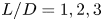 $L/D=1,2,3$ is also plotted. The length of the recirculation zone closely follows the neutral stability curve of the symmetry breaking mode (i.e.
 $\lambda _r^{SB}=0$) when it is smaller than
 $L/D$, indicating that the emergence of this mode is closely linked to the flow structure related to the zone (Lacis et al. Reference Lacis, Brosse, Ingremeau, Mazzino, Lundell, Kellay and Bagheri2014). When the size of the zone becomes greater than the given
 $L/D$, it deviates from
 $\lambda _r^{SB}=0$ considerably and the slope of its growth with respect to
 $Re$ becomes similar to that of (3.1) given for the case without the splitter plate.
3.1. Symmetry breaking mode
We first study the stability and the sensitivity of the symmetry breaking mode. Apart from the strong correlation of the emergence of this mode with the length of the recirculation zone, it has consistently been found that this mode is most unstable for  $L/D \simeq 1$ (see figure 6). Therefore, in this section we will focus on the case of
 $L/D=1$, while discussing the other
 $L/D$ if necessary.
3.1.1. Linear stability
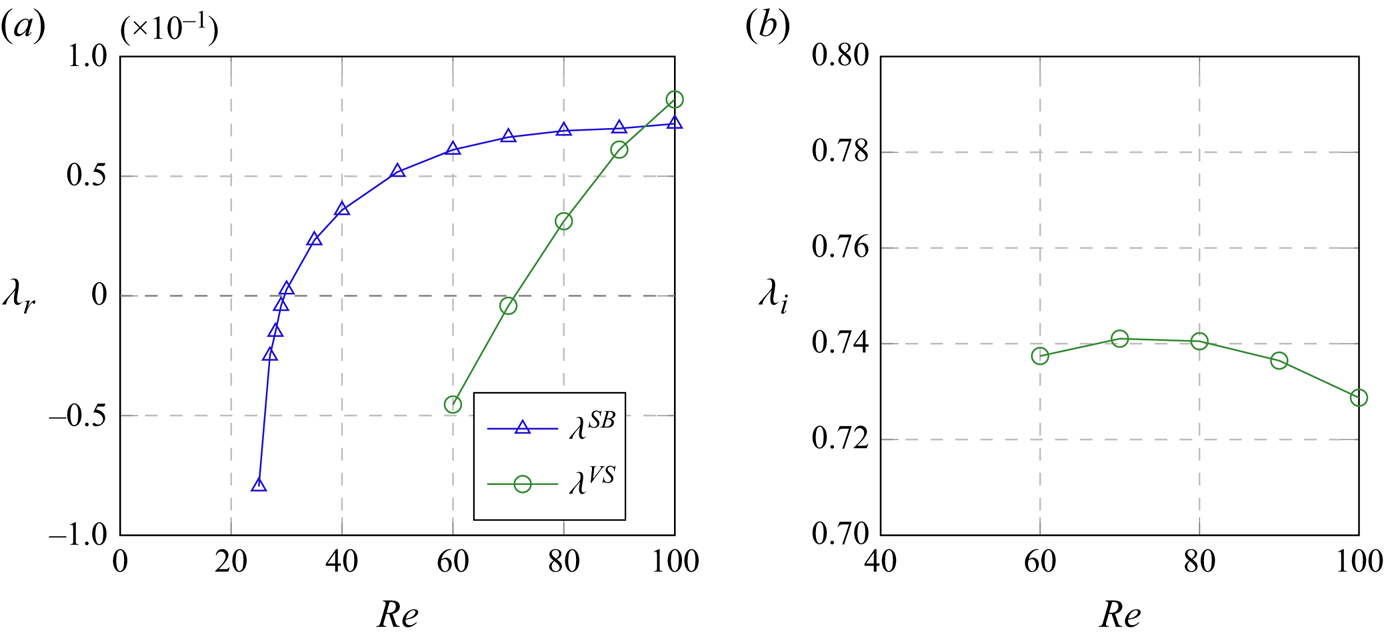
Figure 4 presents the variation of the two leading eigenvalues (symmetry breaking mode and vortex shedding mode) in a range of Reynolds number from  $Re=20$ to
 $Re=100$ for a fixed splitter length of
 $L/D=1$. In figure 4(a) we observe that the symmetry breaking mode is the instability emerging at the lowest Reynolds numbers, as was also highlighted in figure 3. We note that, for
 $Re>70$, the vortex shedding mode is also unstable, if the cylinder is held fixed. However, if it is not initially fixed, the symmetry breaking mode would have been initiated. Therefore, in this case, a competition between the two modes will emerge in transition to a nonlinear state which will depend on how the two modes are nonlinearly coupled and are initiated.
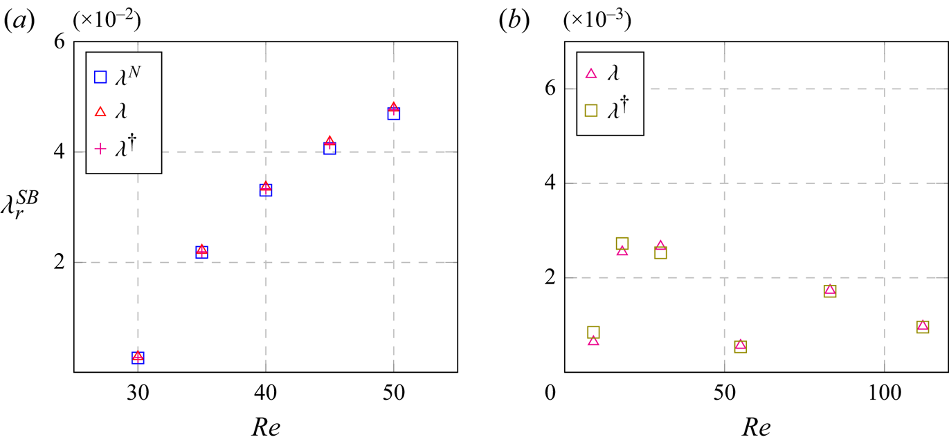
The linear (a) growth rate and (b) frequency of symmetry breaking mode ( $\lambda ^{SB}$) and vortex shedding mode (
 $\lambda ^{VS}$) as a function of the Reynolds number (
 $L/D=1$,
 $I_\theta =50$,
 $U_R=3937$). Note that the frequency of the symmetry breaking mode is not drawn in (b), since
 $\lambda ^{SB}_i=0$.

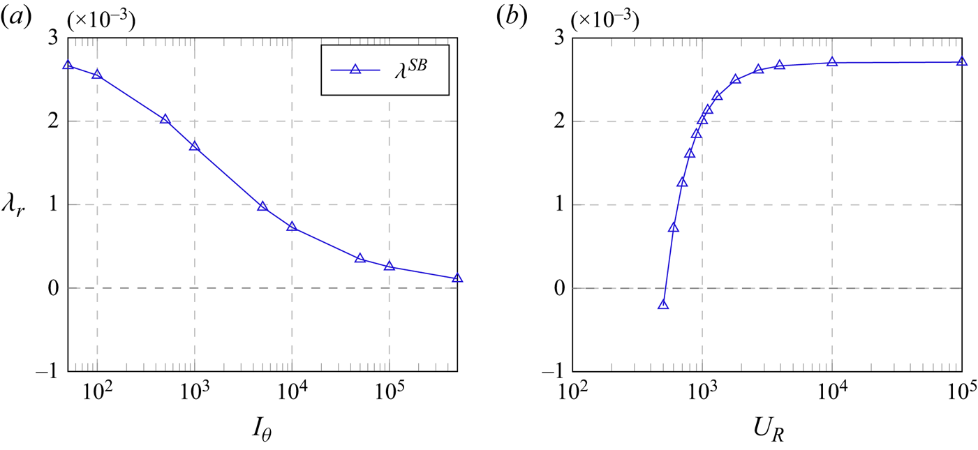
In figure 5 we consider the behaviour of the symmetry breaking mode with respect to the changes in the structural parameters  $I_\theta$ and
 $U_R$ (or, equivalently, the torsional spring stiffness) for a fixed splitter plate length of
 $L/D=1$ at
 $Re=30$. Figure 5(a) shows that the linear growth rate of the symmetry breaking mode remains always positive for all
 $I_\theta$ considered, while it tends to decrease on increasing
 $I_\theta$. This observation is consistent with (2.4a), where
 $I_\theta$ appears to effectively control the strength of the coupling between fluid and structural motions: the higher
 $I_\theta$ is, the weaker the coupling is. This observation also suggests that the symmetry breaking mode is indeed a consequence of FSI. We expect that the symmetry breaking mode will eventually be stabilised in the limit of infinitely large
 $I_\theta$, because the fully rigid cylinder will not allow for any structural motion. Figure 5(b) shows that the growth of the symmetry breaking mode changes very little above a reduced velocity
 $U_R \simeq 4000$. As
 $U_R$ is reduced from this value, the growth rate quickly decreases and eventually becomes stable (negative) at
 $U_R \simeq 520$. This is a simple physical consequence of the fact that the rotational motion of the body is prevented by a very stiff torsional spring – note that the rigid case is given in the limit of
 $U_R \rightarrow 0$.
The linear growth rate of symmetry breaking mode ( $\lambda ^{SB}$) at
 $Re = 30$ and
 $L/D=1$, as a function of (a) inertia for
 $U_R = 3937$ and (b) reduced velocity for
 $I_\theta =50$.

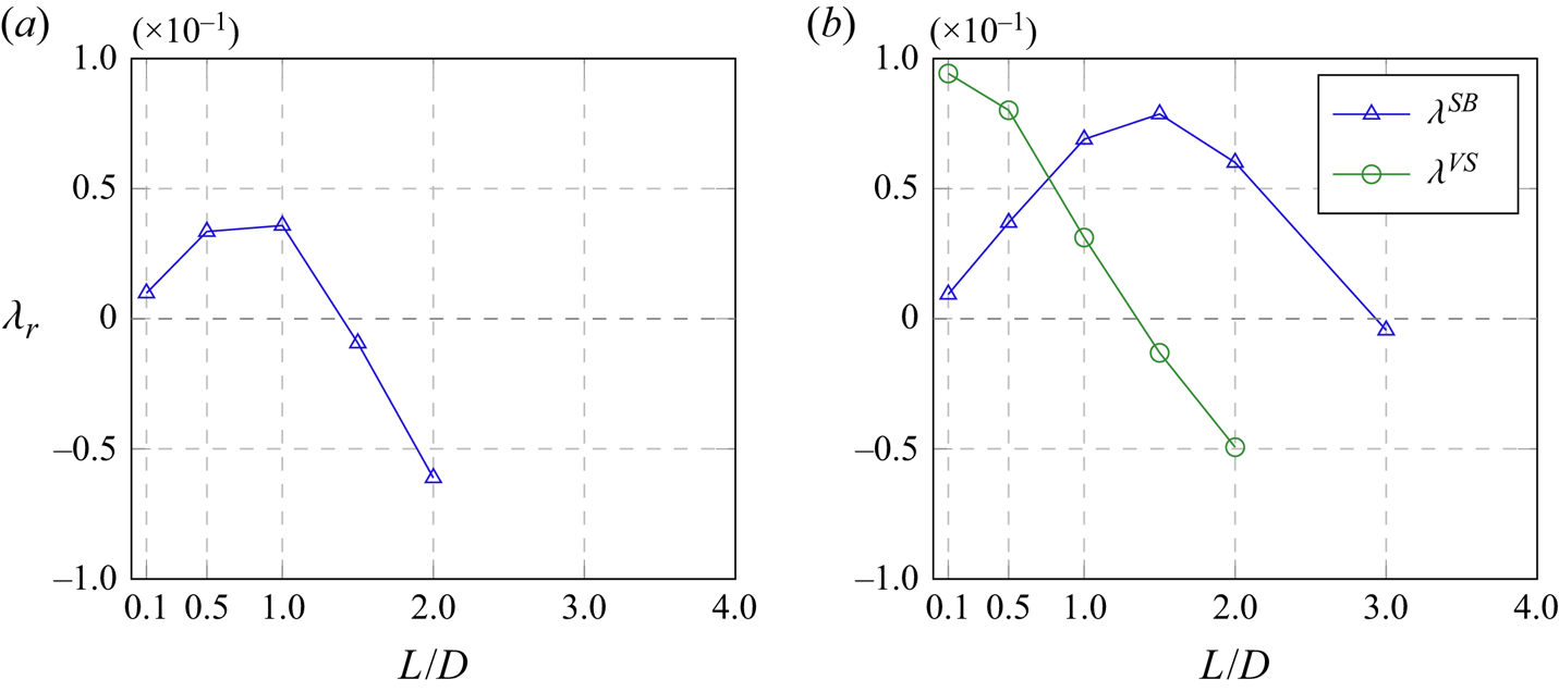
Figure 6 shows the variation of the growth rate of the symmetry breaking mode as a function of the splitter plate length  $L/D$ at two different Reynolds numbers. In figures 6(a) and 6(b) we observe that, for
 $L/D < 1$, the symmetry breaking mode is stabilised as the splitter plate length
 $L/D$ decreases. This would physically be anticipated since the body shape becomes a circular cylinder as
 $L/D \rightarrow 0$. In figure 6(b) we observe that the vortex shedding mode grows faster than the symmetry breaking mode for
 $L/D < 0.75$. This implies that the flow is most likely to transition through the fluid instability mode before the structural mode, if the angle of the cylinder is initially placed to be
 $\theta =0$ at the given Reynolds number,
 $Re=80$. This is not immediately clear from the neutral stability curve in figure 3. However, one must recall that if the flow at a Reynolds number of
 $Re=80$ is realised by increasing the flow speed, the flow regime would change along a horizontal line in figure 3 for a fixed
 $L/D$. In this case, the flow would first experience the symmetry breaking mode at a lower Reynolds number. This implies two possibly different routes of the transition to the final fully nonlinear state at
 $Re=80$. Understanding of the detailed transition dynamics needs a further nonlinear analysis, which is beyond the scope of the present study. Lastly, figure 6 also indicates that there exists a specific splitter plate length, at which the growth rate of the symmetry breaking mode becomes maximum. This length appears to be around
 $L/D \simeq 1$ for the two Reynolds numbers
 $Re=40$ and
 $Re=80$.
The linear growth rate of symmetry breaking mode ( $\lambda ^{SB}$) and vortex shedding mode (
 $\lambda ^{VS}$) as a function of the plate length
 $L/D$ (
 $I_\theta =50$): (a)
 $Re=40$; (b)
 $Re=80$.

3.1.2. Physical mechanism of instability
To understand how the symmetry breaking mode is initiated, the structural part of (2.9) is now rearranged to examine what physical quantities drive the instability. In particular, as presented in more detail in Appendix C, the eigenvalue  $\lambda$ is decomposed into the structural and fluid components
 $\lambda ^{S}$ and
 $\lambda ^{F}$, respectively, such that
 \begin{equation} \lambda = \underbrace{-\frac{\boldsymbol{q}_S^{H} \boldsymbol{W}_S \boldsymbol{L}_{S}\boldsymbol{q}_S}{\boldsymbol{q}_S^{H} \boldsymbol{W}_S \boldsymbol{q}_S}}_{\lambda^S} + \underbrace{\frac{\boldsymbol{q}_S^{H} \boldsymbol{W}_S \boldsymbol{M}_z}{\boldsymbol{q}_S^{H} \boldsymbol{W}_S \boldsymbol{q}_S}}_{\lambda^{F}}, \end{equation}
where  $\boldsymbol {q}_S=[\hat {\theta }\enspace \hat {\phi }]^\textrm {T}$ is the vector containing the structure variables,
 $\boldsymbol {L}_{S}$ the structural part of the operator
 $\boldsymbol {L}$ defined in (2.9),
 $\boldsymbol {M}_z = [\boldsymbol {0}\enspace \hat {\boldsymbol {m}}_z]^\textrm {T}$ with
 $\hat {\boldsymbol {m}}_z=[\hat {m}_{z,p}\enspace \hat {m}_{z,\nu }]^\textrm {T}$ the moment matrix defined in (2.9) as part of the global operator
 $\boldsymbol {L}$, and
 $\boldsymbol {W}_S$ is the weight matrix defined in (A1a). Without the presence of the structural damping parameter (i.e.
 $\zeta _\theta = 0$), the growth rate structural contribution
 $\lambda ^{S}$ is identically 0 and we obtain
 \begin{equation} \lambda = \lambda^F = \lambda_p + \lambda_\nu, \end{equation}
where  $\lambda _p$ and
 $\lambda _\nu$ indicate the contributions from pressure and viscous stress, respectively (see (2.4c) and (2.4d)).
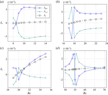
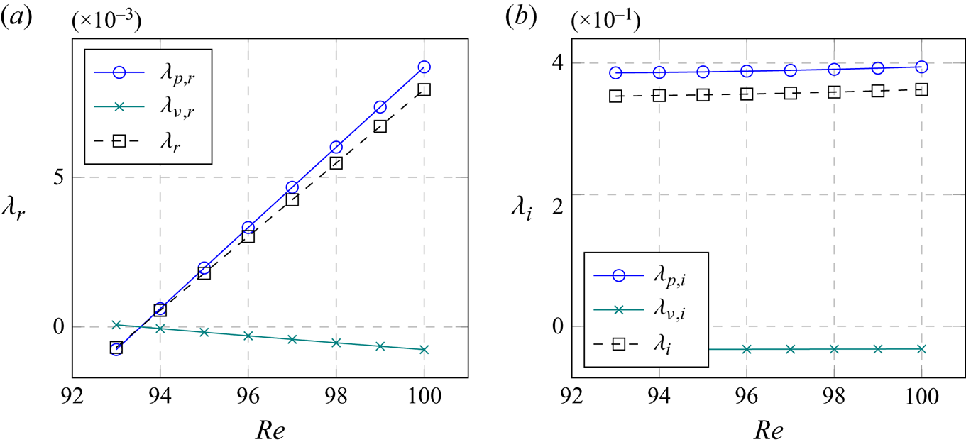
In figure 7 we report how the torque from pressure and viscous stress contributes to the symmetry breaking mode as  $Re$ changes, i.e. the contributions of
 $\lambda _{p,r}$ and
 $\lambda _{\nu ,r}$ to
 $\lambda _{r}$. We first consider relatively short plates (
 $L/D=0.1,0.5$ in figure 7a,b). When
 $Re$ is lower than that for the onset of the symmetry breaking instability, the pressure stabilises the flow while the viscous stress plays a destabilising role at low Reynolds numbers. As
 $Re$ is increased, this balance reverses near the onset of the instability. In this case, the pressure drives the instability and the viscous stress plays a stabilising role, and this remains the dominant behaviour forming the symmetry breaking instability with a further increase of
 $Re$. The predominance in the destabilising role of pressure is also seen for longer plates (
 $L/D=1,2$; figure 7c,d), when
 $Re$ is sufficiently larger than that for the onset of the instability. However, in this case, there is also a range of
 $Re$, in which the pressure stabilises the mode, while the viscous stress destabilises it, for example,
 $Re \simeq 30$ for
 $L/D=1$ (figure 7c) and
 $55 \lesssim Re \lesssim 65$ for
 $L/D=2$ (figure 7d). The observations made here suggest that the balance between the pressure and viscous stress plays a crucial role in the symmetry breaking mode. We note that the change of the pressure and stress balance with
 $Re$ is likely to be associated with the recirculation zone in the near-wake region, given that the length of the recirculation zone is approximately linearly proportional to
 $Re$ (see (3.1)).
Componentwise contributions to the instability growth rate (see (3.3)):  $\lambda _{p,r}$, pressure;
 $\lambda _{\nu ,r}$ viscous stress;
 $\lambda _{r}$ the growth rate as a function of the Reynolds number. Here, (a)
 $L/D=0.1$; (b)
 $L/D=0.5$; (c)
 $L/D=1$; (d)
 $L/D=2$.

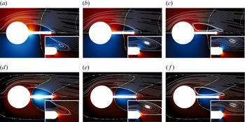
To understand how the symmetry breaking mode is associated with the recirculation zone, in figure 8, we further examine the symmetry breaking mode in relation to the flow structure of the recirculation zone for  $L/D=1$. Figure 8 shows the pressure
 $p$ and vorticity
 $\omega _z$ distributions of the eigenmode presented for an instability with a counter-clockwise rotation of the cylinder at
 $Re=30, 32$ and
 $34$. From figure 7(c) we observe this is just after the onset on the symmetry breaking instability and covers the range where the roles of pressure and viscous stress are interchanged. In these plots the streamline of base flow is also indicated to visualise the recirculation bubble. For all
 $Re$ considered, we observe that the flow features are relatively similar although slightly changing in magnitude. The data are normalised so that the maximum value of the pressure and velocity magnitude are set to one. First considering the pressure distribution where we note the moment is generated by normal forces acting on the splitter plate, since the centre of rotation is at the centre of the cylinder so that no contribution is provided to the moment from the cylinder surface. There is a stabilising clockwise moment being generated by the pressure force on the inner part of the splitter plate from the root of the plate to approximately its midpoint. Analogously there is then a destabilising counter-clockwise pressure force acting from approximately the middle of the plate to the tip. As shown in figure 7, at
 $Re=30$ the contribution to the clockwise moment is larger but this swaps over to a counter-clockwise pressure contribution at
 $Re=32$ and
 $34$. This change in sign is rather subtle and is not associated with any significant change in the structure of the pressure distribution but rather a change in the magnitude of each contribution (figure 8a–c).
(a–c) Pressure and (d–f) spanwise vorticity of the eigenmode of symmetry breaking instability for  $L/D=1$ at (a,d)
 $Re=30$, (b,e)
 $Re=32$ and (c, f)
 $Re=34$. Here, the red and blue colours denote positive and negative values, respectively, and their brightness indicates the magnitude. The continuous lines are associated to the base flow streamlines for the corresponding Reynolds numbers and the dotted contours represent the 0-isocontour of the perturbed fields.

A similar observation can be made from the vorticity plots and the contribution towards the viscous moment component (figure 8d–f). We have chosen to plot vorticity since the vorticity is the negative of the strain tensor at the surface of the body and so the tangential direction of the shear stress force can be inferred as the negative of the dynamics viscosity multiplied by the vorticity. On the upper surface of the splitter plate where we observe negative vorticity the viscous shear stress is therefore acting in the positive  $x$-direction and analogously the negative vorticity on the lower surface of the splitter plate (where the surface normal is now negated) is associated with a shear stress in the negative
 $x$-direction. These shear components act over a large portion of the splitter plate surface and together generate a clockwise moment on the body. However, the magnitude of this moment is associated with a moment arm that is only half the thickness of the splitter plate. Correspondingly, the positive vorticity on the cylinder surface and at the tip of the splitter plate are associated with a surface shear stress that generates a counter-clockwise contribution to the moment where the moment arm around the cylinder is equal to the radius and the moment arm at the tip is obviously equal to the splitter plate length plus the radius. Once again there is a subtle balance between these two contribution where at
 $Re=30$ the counter-clockwise contribution from the cylinder and tip dominate but at
 $Re=32,34$ the clockwise contribution from the plate is larger but relatively balanced. As with the pressure distribution there is no significant change in structure with the change in Reynolds number.
Interestingly, as the symmetry breaking mode becomes unstable with increasing  $Re$, the original recirculation bubble appears to develop a stronger secondary daughter bubble near the tip with its increased size (see the inset of figure 8a–c). This further suggests the importance of the structure of the base flow at the tip of the plate, as we shall also see in the sensitivity analysis. This observation is also in agreement with the early experimental study (see Toebes & Eagleson Reference Toebes and Eagleson1961), where vortex-induced vibrations of thin flat plates were studied as a function of the trailing edge geometry and the motion's responses were reported to be largely sensitive to this parameter.
3.1.3. Adjoint sensitivity
We next consider the sensitivity of the symmetry breaking mode. The adjoint perturbation velocity field  $\hat {\boldsymbol {u}}^{\dagger} (x,y)$ represents the sensitivity to an open-loop body forcing in a weakly nonlinear regime, whereas
 $\varTheta _F(x,y)$ indicates the sensitivity to a small forcing in the form of a localised feedback (Chomaz Reference Chomaz2005; Giannetti & Luchini Reference Giannetti and Luchini2007). In particular, the sensitive region characterised by
 $\varTheta _F(x,y)$ has often been referred to as the ‘wavemaker’ region for the vortex shedding mode.
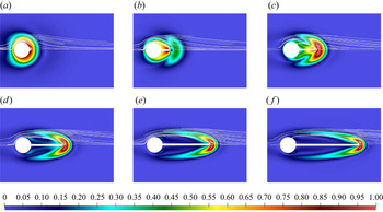
Figure 9 shows the amplitude of the adjoint mode  $\| \hat {\boldsymbol {u}}^{\dagger} (x,y)\|_2$. The shape of the adjoint mode changes notably as a function of the plate length. For shorter splitter plate lengths (
 $L/D < 1.5$), the peak of the adjoint mode amplitude is most energetic around the cylinder and splitter plate boundary, whereas for longer plates
 $(L/D >1.5)$, it becomes detached and appears slightly downstream of the tip of the splitter plate. It should be mentioned that the localisation of the adjoint mode amplitude near the tip of the splitter plate in figure 9 cannot be a consequence of increasing Reynolds number. Indeed, while the role of the advection increases with
 $Re$, it should be noted that the adjoint operator has advection towards upstream. Therefore, the consistent localisation of the adjoint mode around the tip is presumably a consequence of the increasing length of the splitter plate, because exerting a force at the tip would lead to the largest torque to the cylinder.
Isocontours of the amplitude of the adjoint eigenmode of the symmetry breaking mode near the point of instability: (a)  $L/D=0.1$ at
 $Re=9$, (b)
 $L/D=0.5$ at
 $Re=18$, (c)
 $L/D=1.0$ at
 $Re=30$, (d)
 $L=2.0$ at
 $Re=55$, (e)
 $L/D=3.0$ at
 $Re=83$, ( f)
 $L/D=4.0$ at
 $Re=112$, (g) colour bar. Here, the contour levels are normalised by the peak adjoint mode amplitude.

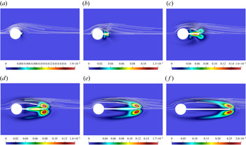
Analogous to figure 9 in 10, we plot isocontours of the sensitivity to a spatially localised feedback  $\varTheta _F$ along the instability threshold for different splitter plate lengths. In this figure, as we increase
 $L/D$, the spatial location of the most sensitive region is also shifted downstream due to the adjoint mode shown in figure 9. For
 $L/D < 1$, the sensitive region is located mostly along the splitter plate, whereas for
 $L/D > 1$, the highest sensitivity region is found to emerge at the end of the splitter plate. For
 $L/D=1$, we observe that both of the regions are equally energetic.
The sensitivity to spatially localised feedback  $\varTheta _F$ of the symmetry breaking mode near the onset of the instability: (a)
 $L/D=0.1$ at
 $Re=9$, (b)
 $L/D=0.5$ at
 $Re=18$, (c)
 $L/D=1.0$ at
 $Re=30$, (d)
 $L=2.0$ at
 $Re=55$, (e)
 $L/D=3.0$ at
 $Re=83$, ( f)
 $L/D=4.0$ at
 $Re=112$.

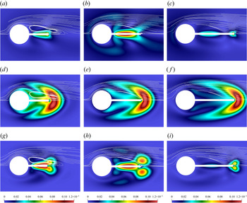
Finally, we compare the direct mode, adjoint mode and sensitivity to localised feedback  $\varTheta _F$ for three different splitter plate lengths
 $L/D=1,1.5,2$ at
 $Re=40$, and this is shown in figure 11. The three plate lengths correspond to unstable (
 $L/D=1.0$), marginally stable (
 $L/D=1.5$) and stable (
 $L/D=2.0$) conditions, respectively. The first row of plots (i.e. figure 11a–c) shows the perturbed velocity field amplitude
 $\| {\hat {\boldsymbol {u}}} \|_2$, the second row of plots (i.e. figure 11d–f) presents the adjoint velocity field amplitude
 $\|\hat {\boldsymbol {u}}^{\dagger} \|_2$, and the last row of plots (i.e. figure 11g–i) show the corresponding sensitivity to localised feedback
 $\varTheta _F(x,y)$. In all the cases, the region of large
 $\| \hat {\boldsymbol {u}} \|$ is located mostly around the splitter plate. For the longest plate
 $L/D=2$, it also shows large intensity localised around the tip. The adjoint velocity field
 $\| \widehat {\boldsymbol {u}}^{\dagger} \|$ consistently exhibits the peak near the tip in all the cases (figure 9d–f). As
 $L/D$ is increased, the peak region also consistently shifts downstream along with the tip location. The sensitivity field
 $\varTheta _F(x,y)$, which is a combination of the previous two fields, has a peak amplitude around the plate midpoint at
 $L/D=1$. As
 $L/D$ is increased,
 $\varTheta _F(x,y)$ around the tip gradually becomes large. When
 $L/D=2$, it exhibits its peak only around the splitter plate tip. It is interesting to note that when
 $\varTheta _F(x,y)$ appears to be distributed around the entire splitter plate for
 $L/D=1$ and
 $L/D=1.5$. In this case, the symmetry breaking mode is highly unstable (
 $L/D\simeq 1.0$; see also figure 6). In any case, the importance of the flow around the tip is clearly well visible in the sensitivity analysis in this section, and this is consistent with the discussion in § 3.1.2. Finally, the sensitivity to the structural parameters
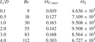
 $\varTheta _S$ are compared with the maximum value of
 $\theta _F$ in table 1. In all the cases investigated, the symmetry breaking mode has been found to be much more sensitive to the structural parameters, indicating that the symmetry breaking mode can easily be controlled by the structural damping and stiffness.
Values of  $\varTheta _{F,max}(\equiv max_{\boldsymbol {x}}|\varTheta _F|)$ and
 $\varTheta _S$ along the threshold of stability as a function of the splitter plate length. The cases here correspond to those in figure 10.

Comparison of the magnitude of (a–c) the direct mode  $\| \hat {\boldsymbol {u}} \|$, (e–f) the magnitude of the adjoint mode
 $\| \hat {\boldsymbol {u}}^{\dagger} \|$ and (g–i) the sensitivity to localised forcing
 $\varTheta _F$ for different plate lengths at
 $Re=40$. Here, (a,d,g)
 $L/D=1$, (b,e,h)
 $L/D=1.5$, (c, f,i)
 $L/D=2$.

3.2. Torsional flapping
For longer splitter plate lengths ( $L/D>3$), the leading instability is no longer the symmetry breaking mode, as shown in figure 3. Unlike the stationary symmetry breaking mode which has a purely real eigenvalue, the eigenvalue of this mode has a non-zero imaginary part, indicating that it is an oscillatory/dynamic instability. Furthermore, the neutral stability curve of this mode in figure 3 does not seem to be correlated with the length of the recirculation zone, indicating that its origin is not necessarily related to the separation of the flow. As will be discussed later, this mode appears to share many similarities to the flapping instability of flag (see the review by Shelley & Zhang Reference Shelley and Zhang2011). We shall therefore refer to this mode as torsional flapping.
3.2.1. Linear stability
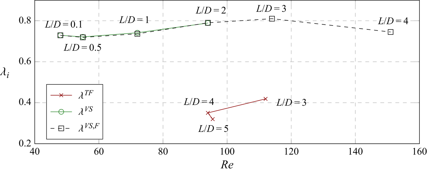
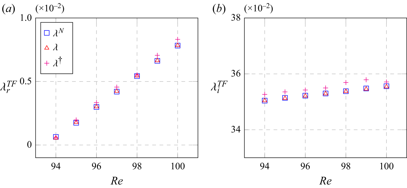
We first explore the linear stability characteristics of the torsional flapping mode. Figure 12 plots the linear frequency of the instability mode as a function of Reynolds number for different splitter plate lengths, and compares it to that of the vortex shedding mode with or without FSI. Here, the frequencies are obtained when the modes are close to neutral stability (i.e.  $\lambda _r\simeq 0$). Regardless of the coupling with structural motion, the frequency of the vortex shedding mode always stays around
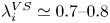 $\lambda _i^{VS} \simeq 0.7\text {--}0.8$ for all the values of
 $L/D$ considered. As mentioned previously, the torsional flapping mode only appears for sufficiently long plates (
 $L/D \geq 3$ in this study). The frequency of the flapping mode (
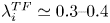 $\lambda _i^{TF} \simeq 0.3\text {--}0.4$) is found to be lower than that of the vortex shedding mode (
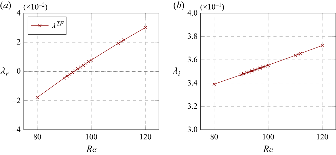
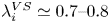 $\lambda _i^{VS} \simeq 0.7\text {--}0.8$), although they both are in the same order of magnitude. Finally, the frequency of the flapping mode is found to change little with variation of the Reynolds number (equivalently the length of the recirculation zone), as shown in figure 13.
The linear frequency of torsional flapping mode and vortex shedding mode as a function of the Reynolds number ( $I_\theta =50$,
 $L/D=0.1$ to 4,
 $U_R = 3937$). Here,
 $\lambda _r \simeq 0$.

Linear (a) growth rate and (b) frequency of the torsional flapping mode as a function of the Reynolds number ( $I_\theta =50$,
 $L/D=4$,
 $U_R = 3937$).

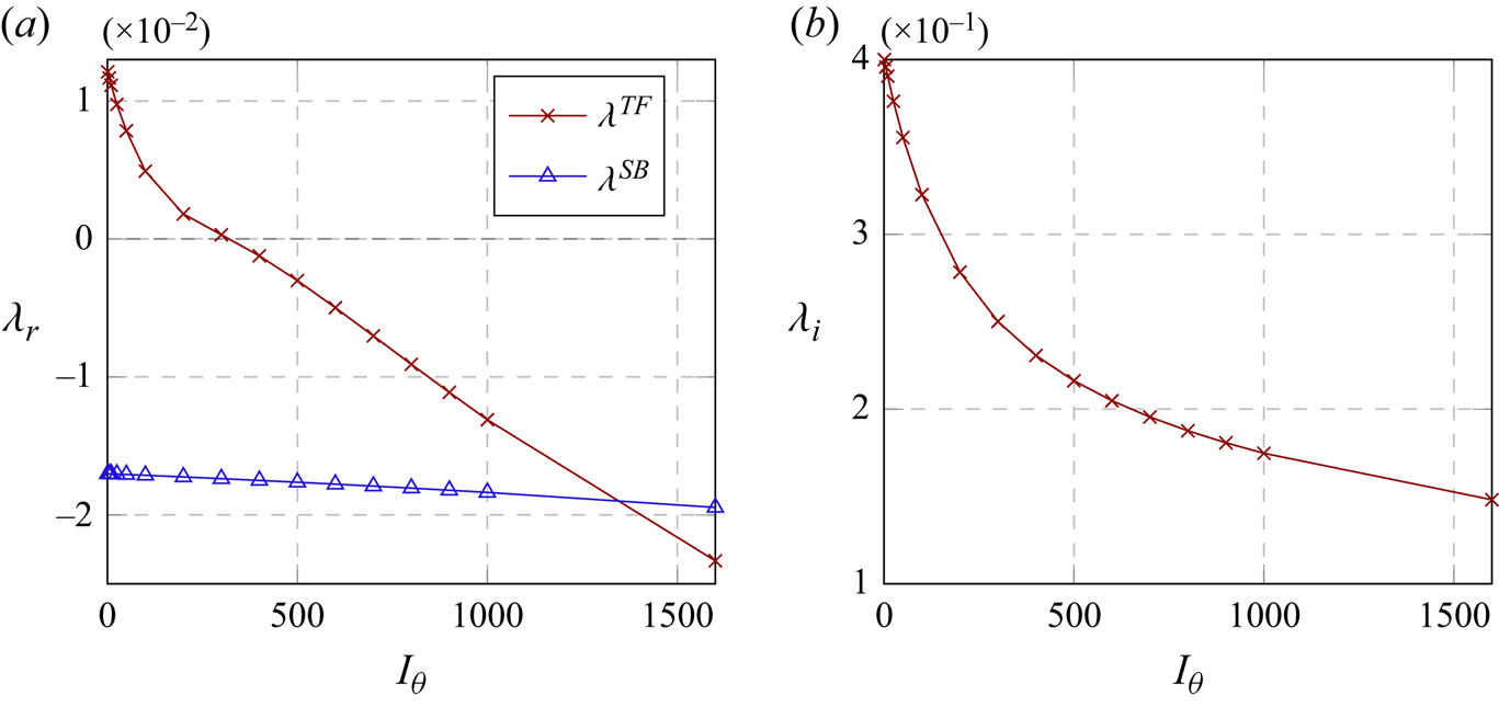
The change of the eigenvalue of the torsional flapping mode with the inertia  $I_\theta$ is also reported with that of the symmetry breaking mode in figure 14. We observe that the growth rate of the torsional flapping mode is reduced on increasing
 $I_\theta$ from a very low value (
 $I_\theta =1)$ and that the mode is completely stabilised at
 $I_\theta \simeq 300$ (figure 14a). We note that the stabilisation of the flapping mode with increasing
 $I_\theta$ is more rapid than that of the symmetry breaking mode. Therefore, it remains more stable than the symmetry breaking mode when
 $I_\theta$ is sufficiently great (
 $I_\theta \gtrsim 1300$ in this case). Finally, we also observe that the frequency of the flapping mode decreases as
 $I_\theta$ is increased.
Variation of linear (a) growth rate and (b) frequency of the torsional flapping ( $\lambda ^{TF}$) and the symmetry breaking mode (
 $\lambda ^{SB}$) with the dimensionless inertia
 $I_\theta$ (
 $L/D=4$,
 $U_R = 3937$,
 $Re=100$).

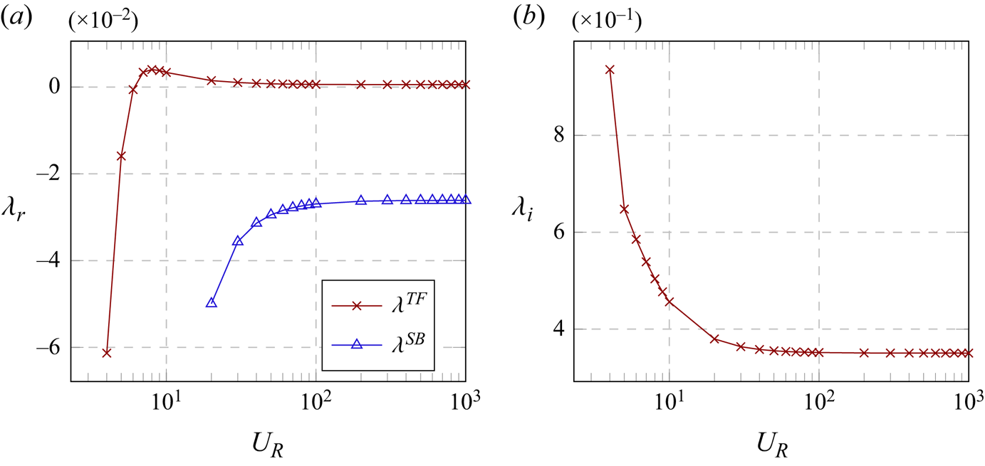
In figure 15 we show the variation of the linear growth rate and frequency of the torsional flapping mode,  $\lambda ^{TF}$, at
 $Re=94$ (the critical Reynolds number is
 $Re \simeq 93.5$ in this case) for a plate length
 $L/D=4$, with regards to the change in reduced velocity
 $U_R$. In the same figure 15(a) we also present the growth rate of the symmetry breaking mode for comparison. Both of the instabilities appear to be insensitive, both in terms of growth rates and frequency, to the change in reduced velocity around the reference value studied in this work (i.e.
 $U_R=3937$). For low values of
 $U_R$, the growth rate of the torsional flapping mode displays a small increase up to a local maximum value around
 $U_R \simeq 8$ before sharply decreasing as
 $U_R \rightarrow 0$ (i.e. a rigid body configuration). This behaviour differs from that of the symmetry breaking mode which is monotonically stabilised as
 $U_R \rightarrow 0$.
Variation of linear (a) growth rate and (b) frequency of the torsional flapping ( $\lambda ^{TF}$) and the symmetry breaking mode (
 $\lambda ^{SB}$) with the reduced velocity
 $U_R$ (
 $L/D=4$,
 $I_\theta = 50$,
 $Re=94$).

3.2.2. Physical mechanism of instability
Now, we explore the underlying physical mechanism of this oscillatory instability. Similarly to the symmetry breaking mode analysis in § 3.1.2, we consider the pressure and viscous stress contributions to the torsional flapping mode  $\lambda ^{TF}$ and this is shown in figure 16 for
 $L/D=4$. It is evident that the flapping mode is predominantly driven by pressure, while the viscous stress plays a stabilising role in this oscillatory instability.
Componentwise contributions to the instability (a) growth rate and (b) frequency as a function of the Reynolds number for  $L/D=4$ (see (3.3)):
 $\lambda _{p,r}$,
 $\lambda _{p,i}$ pressure;
 $\lambda _{\nu ,r}$,
 $\lambda _{\nu ,i}$ viscous stress;
 $\lambda _{r}$,
 $\lambda _{i}$ the growth rate and frequency. Here, the critical Reynolds number for the onset of the instability is
 $Re_c \simeq 93.5$.

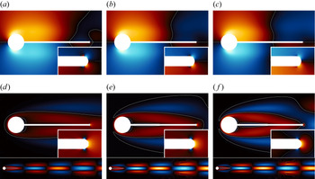
Pressure and spanwise vorticity fields of the torsional flapping mode are visualised at three different Reynolds numbers ( $Re=92,94,96$; note the critical Reynolds number for the onset of the instability is
 $Re_c\simeq 93.5$) in figure 17, where the phase of the eigenmode is set for a time instance of counter-clockwise rotation of the cylinder. First, given that the pressure generates the moment acting in the surface normal direction, only the pressure distribution around the plate can cause the rotation of the cylinder (see also the discussion in § 3.1.2 for the symmetry breaking mode). In all three cases, it is seen that the pressure distribution from the root of the plate to approximately the midpoint creates a moment in the clockwise direction, indicating its stabilising role in the rotation of the cylinder caused by the instability (figure 17a–c). In contrast, the tip pressure distribution generates a moment in the counter-clockwise direction, thereby being the key mechanism of the instability. Indeed, as
 $Re$ is increased, the region with the destabilising pressure distribution in the near tip becomes wider with more elevated intensity. Second, the eigenmode of the flapping mode shows a symmetric distribution of the spanwise vorticity about
 $y=0$ (figure 17d–f). This indicates that the moments generated by most of the viscous shear stress in the upper and the lower part of the plate would be cancelled out by each other. Therefore, the main contribution of the viscous shear stress to the moment would arise from the front stagnation point of the cylinder and from the tip of the plate. The visualisation of the eigenmode reveals that the vorticity at the front stagnation point is much smaller than that at the tip. Also, the tip has a much longer moment arm than the front stagnation point, indicating the importance of the tip vorticity distribution. For the cylinder rotating in the counter-clockwise direction due to the flapping mode instability, the positive spanwise vorticity near the tip indicates the stabilising role of the viscous shear stress, consistent with figure 16. Furthermore, the downstream vorticity right next to the region of the positive vorticity near the tip is negative (i.e. clockwise direction), indicating the emergence of a vortical structure rotating in the counter-clockwise direction in accordance with the Kelvin's circulation theorem.
(a–c) Pressure and (d–f) spanwise vorticity of the eigenmode of the symmetry breaking instability for  $L/D=4$ at (a,d)
 $Re=92$, (b,e)
 $Re=94$ and (c, f)
 $Re=96$. Here, the red and blue colours denote positive and negative values, respectively, and their brightness indicates the magnitude. The white contour lines indicate
 $\hat {p}=0$ and
 $\hat {\omega }_z=0$.

Let us now summarise the key features of the oscillatory instability discussed so far. First, the instability appears when the length of the splitter plate is sufficiently long. Importantly, the neutral stability does not show any correlation with the length of the recirculation zone (figure 3), indicating that the origin of this instability is not necessarily related to the recirculation zone in the near wake. Second, the instability mode frequency increases, as the mass of the plate is gradually reduced from a large value (figure 14). Third, the mode is stabilised by increasing the stiffness (figure 15). Finally, the mode is destabilised primarily due to pressure acting on the tip of the plate, while the viscous stress merely stabilises the mode (figure 16).
These features can be compared with those observed in a simple model for the flapping (or flutter instability) for the flag and elastic plate immersed in an inviscid uniform flow (see the analysis on page 455 in Shelley & Zhang Reference Shelley and Zhang2011). The dispersion relation of their model is given by
 \begin{equation} (\omega+k)^2=\tfrac{1}{2}({-}R_1|k|^2\omega^2+R_2|k|^5), \end{equation}
where  $k$ is the spatial streamwise wavenumber of the flag (or plate) and
 $\omega$ the complex frequency for the instability frequency and growth rate,
 $R_1$ the dimensionless inertia of the flag (or plate) and
 $R_2$ its dimensionless stiffness (or rigidity). When (3.4) exhibits an instability, its real frequency (denoted by
 $\omega _r$) is given by
 \begin{equation} \omega_r={-}\frac{2k}{2+R_1|k|} \end{equation}
and the growth rate for instability is proportional to
 \begin{equation} d_k={-}R_1(R_2 |k|^3-2)-2R_2 |k|^2. \end{equation}
For a comparison of this instability with the torsional flapping mode, the wavenumber  $k$ here may be set to be a fixed value (say
 $k \sim O(1/(L+D/2))$) because the cylinder with the splitter plate considered in the present study only admits rotation around the centre. From (3.5b), the instability given by (3.4) arises when
 $L$ is sufficiently large (i.e. when
 $k$ is sufficiently small). The instability frequency in (3.5a) increases on decreasing dimensionless inertia
 $R_1$. The growth rate in (3.5b) also becomes smaller as the dimensionless stiffness
 $R_2$ increases. Lastly, given that the model is based on the inviscid fluid assumption, the fluid force considered in (3.4) is only from pressure (see also Shelley & Zhang Reference Shelley and Zhang2011). It is evident that all these features from this simple model are consistent with those of the torsional flapping instability in the present study (see the paragraph above). It appears that a similar low-frequency instability was also observed in the recent work by Pfister & Marquet (Reference Pfister and Marquet2020), where a flow over a fixed circular cylinder with a flexible plate is studied. However, a direct comparison of this instability mode with that of the model in Shelley & Zhang (Reference Shelley and Zhang2011) is made here for the first time, and it clarifies the origin of this type of instability.
3.2.3. Adjoint sensitivity
Finally, we consider the adjoint sensitivity of the flapping instability mode. Here, we only show the result for  $L/D=4$, as this case is found to be quite similar to that for
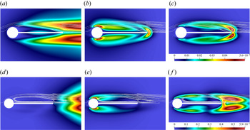
 $L/D=3$. Figure 18 shows the magnitude of the direct
 $\| \hat {\boldsymbol {u}} \|$ and adjoint
 $\| \hat {\boldsymbol {u}}^{\dagger} \|$ modes and the sensitivity to localised forcing
 $\varTheta _F$ for
 $L/D=4$. Here, in each case, the Reynolds number is chosen so as for the corresponding mode to be slightly unstable. Figure 18(a) shows that the velocity perturbation magnitude of the torsional flapping mode is distributed symmetrically about
 $y=0$. The mode exhibits a non-negligibly large perturbation velocity throughout the separating shear layer and it develops the peak value downstream of the plate. This is in contrast to the vortex shedding mode in figure 18(d), which exhibits its perturbation velocity only donwstream of the plate. It is presumable that the large perturbation velocity developed from the separation point is due to the fact that the flapping mode directly involves the motion of the plate, whereas the vortex shedding mode does not require the motion of the plate at least near the onset.
(a,d) Direct mode  $\| \hat {\boldsymbol {u}} \|$, (b,e) adjoint mode
 $\| \hat {\boldsymbol {u}}^{\dagger} \|$ and (c, f) sensitivity to localised forcing
 $\varTheta _F$ for
 $L/D=4$: (a–c) the torsional flapping instability at
 $Re={94}$, (d–f) the vortex shedding instability at
 $Re={151}$. Here, white solid lines indicate streamlines of the corresponding base flow.

An interesting feature of the flapping instability is that the adjoint mode exhibits large values both in the separating shear layer around the plate and near the tip of the plate, as shown in figure 18(b). This feature is distinguished from the adjoint mode of the vortex shedding instability shown in figure 18(e) and the symmetry breaking instability shown in figure 9( f), which have large values only either in the separating shear layer (figure 18e) or near the tip of the plate (figure 9 f). While the tip behaviour of the adjoint mode of the flapping instability is consistent with the discussion in § 3.2.2, its behaviour in the separating shear layers rather resembles that of the vortex shedding mode. This suggests that the structure of the adjoint flapping mode in the separating shear layers might be due to the oscillating nature of the instability like the vortex shedding mode. The sensitivity to localised feedback forcing  $\varTheta _F(\equiv \| \hat {\boldsymbol {u}} \| \,\| \hat {\boldsymbol {u}}^{\dagger} \|$) of the flapping mode is shown in figure 18(c). In this case,
 $\varTheta _F$ are large both in the separating shear layer and near the tip, although the tip region now has the maximum magnitude due to the spatial structure of the direct mode
 $\| \hat {\boldsymbol {u}} \|$ (figure 18a). The overall spatial structure of
 $\varTheta _F$ of the flapping mode is similar to that of the vortex shedding mode, although the tip sensitivity region of the vortex shedding mode is developed further downstream compared with that of the flapping mode. Finally, similarly to the symmetry breaking mode, the flapping mode also shows large sensitivity to the change in the structural parameters, as shown in table 2.
Values of  $\varTheta _{F,max}(\equiv max_{\boldsymbol {x}}|\varTheta _F|)$ and
 $\varTheta _S$ along the threshold of stability as a function of the splitter plate length. Here,
 $\lambda _r^{TF}\simeq 0$.

4. Conclusions
We have studied instabilities and their sensitivity in a flow over a rotationally flexible circular cylinder with a rigid splitter plate. The cylinder is coupled with a spring-mass-damper system at its centre, such that it can rotate in response to the torque applied by the surrounding fluid flow. The theoretical linear stability and sensitivity methodology is derived for a non-rotationally symmetric problem which is observed to be more intricate than the rigid body stability methodology due to the boundary condition coupling of the base flow in the linearised problem. Three types of instabilities have been found: the vortex shedding mode, the symmetry breaking mode and the torsional flapping mode. A particular focus of this study has been given to the understanding of the symmetry breaking and torsional flapping modes which originate from FSI. It was found that the emergence of the symmetry breaking instability mode is strongly correlated with the length of the recirculation zone and the related flow structure near the tip region of the plate. The distribution of the pressure and viscous stress balance of the mode near the root and tip regions of the splitter plate was also found to play a crucial role for the symmetry breaking mode. In particular, as the Reynolds number is increased, the distribution near the tip gradually becomes more important, resulting in destabilistion of the symmetry breaking mode. The importance of the tip region was further identified by the subsequent adjoint sensitivity analysis. An oscillatory instability, which we referred to as ‘torsional flapping’, was also found in this flow. This type of instability has not been widely reported with the only other case we are aware of being in the recent work of Pfister & Marquet (Reference Pfister and Marquet2020) who considered a flexible splitter plate. This instability emerges when the length of the splitter plate is sufficiently large enough ( $L/D\geq 3$ in this study). Unlike the symmetry breaking mode, this instability mode does not appear to be correlated to the length of the recirculation zone. However, the distribution of the pressure and viscous stress balance revealed that flow near the tip region of the plate is also crucial for this mode, and this was also confirmed by the sensitivity analysis. Lastly, all the observed physical features of the oscillatory instability mode were very similar to those of the flapping (or flutter) instability observed in a flag or a flexible plate, indicating that these two instabilities are of the same type.
Perhaps, the most important finding of this work would be the identification of the importance of the flow in the near tip region of the plate for both the symmetry breaking and flapping instabilities. The strong sensitivity, presumably also related to the long moment arm of the region, suggests that the two instabilities originating from FSI can effectively be controlled by carefully modifying the flow in the tip region. This is also consistent with the early experimental study (Toebes & Eagleson Reference Toebes and Eagleson1961) which showed how different shapes of trailing edge of a thin plate can drastically modify the behaviour of the vortex-induced vibration. Therefore, a sensitivity analysis used in this study or with a more specific form of objective functionals (e.g. lift and drag) can further be formulated to optimise the shape of the trailing edge. Finally, as the adjoint fields are now available from this study, they can be used to formulate a weakly nonlinear analysis in a similar manner to Meliga & Chomaz (Reference Meliga and Chomaz2014). Such an analysis would also be useful to identify the competition dynamics between the different instability modes as well as to interpret the results of full nonlinear simulations incorporating the motion of the structure. These are the directions one can pursue, and remain as future work.
Acknowledgements
We are also grateful to Dr O. Marquet who shared a helpful discussion for this work.
Funding
We would like to thank the Brazilian Ministry of Education, Coordenação de Aperfeiçoamento de Pessoal de Nível Superior (CAPES) for the funding that allowed us to conduct this work.
Declaration of interests
The authors report no conflict of interest.
Appendix A. Inner product and adjoint operator
A.1. Inner product
The inner product in the present study is defined for two arbitrary state variables  $\boldsymbol {q}$ and
 $\boldsymbol {m}$, such that
 \begin{equation} \langle {\boldsymbol{q}},{\boldsymbol{m}}\rangle =\underbrace{\int _{ \varOmega } \left( \boldsymbol{q}_F^H\boldsymbol{W}_F {\boldsymbol{m}}_F\right) \text{d}\kern0.06em \boldsymbol{x}}_{\langle \boldsymbol{q}_F,\boldsymbol{m}_F\rangle_F} + \underbrace{\boldsymbol{q}_S^H \boldsymbol{W}_S {\boldsymbol{m}}_S}_{\langle \boldsymbol{q}_S,\boldsymbol{m}_S\rangle_S}, \end{equation}
where the superscript  $(\cdot )^H$ indicates the complex conjugate transpose, and the subscripts
 $_F$ and
 $_S$ indicate the variables for fluid and structure, respectively, e.g.
 $\boldsymbol {q}_F=[\boldsymbol {u}\enspace p]^\textrm {T}$ and
 $\boldsymbol {q}_S=[\theta \enspace \phi ]^\textrm {T}$ for
 $\boldsymbol {q}=[\boldsymbol {u}\enspace p\enspace \theta \enspace \phi ]^\textrm {T}$. The weight matrices are given by
 \begin{equation} \boldsymbol{W}_F = \begin{bmatrix} \boldsymbol{I} & 0 \\ 0 & 0 \end{bmatrix},\quad \boldsymbol{W}_S = \begin{bmatrix} k_\theta & 0 \\ 0 & I_\theta \end{bmatrix}, \end{equation}
where  $\boldsymbol {I}$ is the identity matrix in
 $\mathbb {R}^{2\times 2}$. The choice of this inner product is made so that the corresponding norm physically represents the total energy of the given fluid–structure system, i.e.
 \begin{align} \|{\boldsymbol{q}}\|^2=\langle {\boldsymbol{q}},{\boldsymbol{q}}\rangle &= \int_{\varOmega } \left(\boldsymbol{q}_F^H\boldsymbol{W}_F {\boldsymbol{q}}_F \right) \text{d}\kern0.06em \boldsymbol{x}+ \boldsymbol{q}_S^H \boldsymbol{W}_S {\boldsymbol{q}}_S \nonumber\\ &= \underbrace{\int_{\varOmega}{\left(\bar{\boldsymbol{u}}\boldsymbol{\cdot} {\boldsymbol{u}} \right) \text{d}\kern0.06em \boldsymbol{x}}}_{E_{k,F}} +\underbrace{I_\theta |\phi|^2}_{E_{k,S}}+ \underbrace{k_\theta |{\theta}|^2}_{E_{p,S}}, \end{align}
where  $E_{k,F}$,
 $E_{k,S}$ and
 $E_{p,S}$ are the dimensionless fluid kinetic energy, structural kinetic energy and structural spring-potential energy, respectively.
A.2. Derivation of the adjoint problem
The adjoint operator  $\boldsymbol {L}^{\dagger}$ is defined from
 \begin{equation} \langle \boldsymbol{L} \boldsymbol{q},\boldsymbol{q}^{\dagger} \rangle = \langle \boldsymbol{q},\boldsymbol{L}^{\dagger} \boldsymbol{q}^{\dagger} \rangle + \boldsymbol{B}(\boldsymbol{q},\boldsymbol{q}^{\dagger} ), \end{equation}
and its boundary condition is obtained by enforcing the bilinear concomitant to be zero, i.e.
 \begin{equation} \boldsymbol{B}(\boldsymbol{q}, \boldsymbol{q}^{\dagger} ) = \boldsymbol{0}, \end{equation}
with  $\boldsymbol {q}^{\dagger} = [\hat {\boldsymbol {u}}^{\dagger} \enspace \hat {p}^{\dagger} \enspace \hat {\theta }^{\dagger} \enspace \hat {\phi }^{\dagger} ]^\textrm {T}$ being the adjoint state variable. Expansion of (A3) using (A1a), i.e.
 \begin{align} \langle \boldsymbol{L}{\boldsymbol{q}},{\boldsymbol{q}}^{\dagger} \rangle &= \langle \boldsymbol{F}{\boldsymbol{q}_F},{\boldsymbol{q}}^{\dagger}_F \rangle_F + \langle \boldsymbol{A}{\boldsymbol{q}_F},{\boldsymbol{q}}^{\dagger}_S \rangle_S + \langle {\boldsymbol{S}\boldsymbol{q}_S},{\boldsymbol{q}}^{\dagger}_S \rangle_S \nonumber\\ &= \langle \boldsymbol{q}_F,\boldsymbol{F}^{{{\dagger}}}{\boldsymbol{q}}^{\dagger}_F \rangle_F + \boldsymbol{B}_{F}({\boldsymbol{q}_F},{\boldsymbol{q}}^{{{\dagger}}}_F )+ \langle \boldsymbol{A}{\boldsymbol{q}_F},{\boldsymbol{q}}^{\dagger}_S \rangle_S + \langle {\boldsymbol{q}_S},\boldsymbol{S}^{{{\dagger}}}{\boldsymbol{q}}^{\dagger}_S \rangle_S, \end{align}
with
 \begin{equation} \boldsymbol{L} = \left[\begin{array}{@{}cc@{}} \boldsymbol{F} & \boldsymbol{0} \\ \boldsymbol{A} & \boldsymbol{S} \end{array}\right]\equiv \left[\begin{array}{@{}cccc@{}} \boldsymbol{N} & -\boldsymbol{\nabla} & 0 & 0 \\ \boldsymbol{\nabla}\boldsymbol{\cdot} & 0 & 0 & 0 \\ 0 & 0 & 0 & 1 \\ m_{z,\nu}' & m_{z,p}' & -(2{\rm \pi}/U_R)^2 & -4{\rm \pi} \zeta_\theta/U_R \end{array}\right], \end{equation}
leads to the expressions of
(i) the fluid only adjoint operator
(A7) \begin{equation} \boldsymbol{F}^{\dagger}{=}\left[\begin{array}{cc} \boldsymbol{N}^{\dagger} & -\boldsymbol{\nabla} \\ \boldsymbol{\nabla}\boldsymbol{\cdot} & 0 \end{array}\right] \quad \text{with}\ \boldsymbol{N}^{\dagger} \hat{\boldsymbol{u}}^{\dagger}{=}(\boldsymbol{u}_0 \boldsymbol{\cdot}\boldsymbol{\nabla}) \hat{\boldsymbol{u}}^{\dagger}{-} \left(\boldsymbol{u}_0 \boldsymbol{\nabla}\right)^\textrm{T} \boldsymbol{\cdot} \hat{\boldsymbol{u}}^{\dagger}{+}Re^{{-}1} \nabla^2\hat{\boldsymbol{u}}^{\dagger}; \end{equation}
(ii) the bilinear concomitant from the fluid adjoint operator
(A8)with\begin{equation} \boldsymbol{B}_F\left({\boldsymbol{q}_F},{\boldsymbol{q}}^{{{\dagger}}}_F \right) = \oint _{ \partial \varOmega_S } \underbrace{ \hat{\boldsymbol{u}}^{\dagger} \boldsymbol{\cdot} \left( \sigma' \boldsymbol{\cdot} \boldsymbol{n}_0 \right) }_{\text{gives B.C.}} - \underbrace{\hat{\boldsymbol{u}} \boldsymbol{\cdot} \left( \sigma^{\dagger} \boldsymbol{\cdot} \boldsymbol{n}_0 \right) }_{\text{gives}\ \boldsymbol{A}^{\dagger}}\text{d} l, \end{equation}$\boldsymbol {\sigma }^{\dagger} =-\hat {p}^{\dagger} \boldsymbol {I}+Re^{-1} [\boldsymbol {\nabla } \hat {\boldsymbol {u}}^{\dagger} +(\boldsymbol {\nabla } \hat {\boldsymbol {u}}^{\dagger} )^\textrm {T}]$;(iii) the adjoint structural operator
(A9)\begin{equation} \boldsymbol{S}^{\dagger}{=} \left[\begin{array}{cc} 0 & -1 \\ \left(2{\rm \pi} / U_R \right)^2 & -4{\rm \pi} \zeta_\theta/U_R \end{array}\right]. \end{equation}


The boundary condition at the cylinder interface of the adjoint problem is obtained from the first term on the right-hand side of (A8),
 \begin{align} \oint_{\partial \varOmega_S }\hat{\boldsymbol{u}}^{\dagger} \boldsymbol{\cdot} \left(\boldsymbol{\sigma}' \boldsymbol{\cdot} \boldsymbol{n}_0 \right)\text{d} l &={-}\langle \boldsymbol{A}{\boldsymbol{q}_F},{\boldsymbol{q}}^{\dagger}_S \rangle_S \nonumber\\ &={-}\left(\oint _{ \partial \varOmega_S } \boldsymbol{r}_1 \boldsymbol{\cdot} \left(\boldsymbol{\sigma}' \boldsymbol{\cdot}\boldsymbol{n}_0 \right)\text{d} l\right) \hat{\phi}^{\dagger}, \end{align}
resulting in identification of
 \begin{equation} \hat{\boldsymbol{u}}^{\dagger}(\boldsymbol{r}_0(s))={-}\boldsymbol{r}_1(s) \hat{\phi}^{\dagger} \end{equation}
along the cylinder interface. Finally, the operator  $\boldsymbol {A}^{\dagger}$ is then obtained by writing the second term on the right-hand side of (A8) as
 \begin{align} \oint_{\partial \varOmega_S} \left[- \hat{\boldsymbol{u}} \boldsymbol{\cdot} \left(\boldsymbol{\sigma}^{\dagger} \boldsymbol{\cdot} \boldsymbol{n}_0\right)\right]\text{d} l &= \langle {\boldsymbol{q}_S},\boldsymbol{A}^{\dagger} {\boldsymbol{q}}^{\dagger}_F \rangle_S \nonumber\\ \Leftrightarrow - \boldsymbol{q}_S \boldsymbol{\cdot} \boldsymbol{W}_S \oint _{ \partial \varOmega_S } \boldsymbol{W}_S ^{{-}1} \left[\boldsymbol{\mathcal{B}}\boldsymbol{\cdot} \left( \boldsymbol{\sigma}^{\dagger} \boldsymbol{\cdot}\boldsymbol{n}_0 \right) \right]\text{d} l &= \boldsymbol{q}_S \boldsymbol{\cdot} \boldsymbol{W}_S\boldsymbol{A}^{\dagger} \boldsymbol{q}^{\dagger}_F, \end{align}
where we recall  $\hat {\boldsymbol {u}} = \boldsymbol {\mathcal {B}}\boldsymbol {q}_S$ on
 $\partial \varOmega _S$. This then defines the structural adjoint equation
 \begin{equation} \boldsymbol{A}^{\dagger} {\boldsymbol{q}}^{\dagger}_F ={-}\oint _{ \partial \varOmega_S } \boldsymbol{W}_S ^{{-}1} \left[\boldsymbol{\mathcal{B}} \boldsymbol{\cdot} \left(\boldsymbol{\sigma}^{\dagger} \boldsymbol{\cdot} \boldsymbol{n}_0\right)\right]\text{d}l. \end{equation}
Appendix B. Validation
B.1. Adjoint mode sensitivity to domain dimensions
Although not being the primary subject of this study, the vortex shedding mode developing in the wake of the fixed cylinder plus splitter plate is taken as the validation test case for the minimum domain size required ensuring accuracy of the results for the different splitter plates lengths.
Figures 19 presents the computed numerical values of the real part of the direct and adjoint of the vortex shedding mode eigenvalues as a function of the domain size in the same vertical axis scale. Here, simulations are performed at a Reynolds number close to neutral stability for every plate length, leading to different Reynolds numbers for the different plate lengths. It is noted that the minimum domain dimension required to obtain acceptable agreement between direct and adjoint simulations varies with the splitter plate length, which is presumably a consequence of the effect of the splitter plate length on the structure of the vortex shedding mode. In practice, as the splitter plate length increases, the peak magnitude of the vortex shedding mode is pushed farther downstream, and, hence, a larger domain is required to capture the instability. For numerical efficiency, we carefully chose a different domain size for each splitter plate length to ensure a sufficiently small error between the eigenvalues of direct and adjoint modes:  $200D$ in the downstream direction for
 $L/D \le 2$,
 $300D$ for
 $L/D = 3$ and
 $500D$ for
 $L/D = 4$, respectively.
Comparison of the real part of the computed (a) direct and (b) adjoint eigenvalues for every splitter plate length close to the onset of the instability. Here,  $L/D=0.1$ for
 $Re=47$,
 $L/D=0.5$ for
 $Re=55$,
 $L/D=1.0$ for
 $Re=72$,
 $L/D=2.0$ for
 $Re=95$,
 $L/D=3.0$ for
 $Re=114$ and
 $L/D=4.0$ for
 $Re=151$.

B.2. Symmetry breaking mode
Figure 20 presents the real part of the eigenvalue of the symmetry breaking mode from direct/adjoint analysis and full nonlinear simulation (Serson et al. Reference Serson, Meneghini and Sherwin2016), denoted by  $\lambda$,
 $\lambda ^{\dagger}$ and
 $\lambda ^N$, respectively, while varying the Reynolds number. We note that growth rate from the nonlinear simulation is obtained by fitting the early stage evolution of a small perturbation to an exponential curve. Good agreement is obtained in the range of the Reynolds numbers investigated approximately up to the order of
 $10^{-3}$. We note that a much smaller domain is required to obtain such a good agreement in the case of the symmetry breaking mode: for the results presented in figure 20, the computational domain is given by
 $|y| \leq 20$ and
 $|x|\leq 40$. This is probably due to the fact that in the current formulation and numerical implementation, the nature of the instability starts from the solid itself (i.e. its boundary). Indeed, the peak in the perturbed velocity field is located directly on the boundary (see § 3.1), hence, a smaller domain is enough to capture accurately the mechanism as long as the near-wake base flow is well established. This observation remains true in the case of the torsional flapping mode, as presented below. Having verified the result with the domain of
 $|y| \leq 20$ and
 $|x|\leq 40$, a bigger computational domain (
 $|y| \leq 30$ and
 $|x|\leq 40$) is used for the result in the present study.
Comparison of the real part of the eigenvalue of the symmetry breaking mode from the direct/adjoint mode computations and from full nonlinear simulations: (a)  $L/D=1.0$ for
 $30\le Re \le 50$; (b)
 $L/D=0.1, 0.5, 1.0, 2.0, 3.0, 4.0$ at the Reynolds number near the onset of instability (note that the growth rate is of the order of
 $10^{-3}$). Here,
 $\lambda ^N$ indicates the eigenvalue obtained from full nonlinear simulations, and the domain size is given by
 $|y| \leq 20$ and
 $|x| \leq 40$.

B.3. Torsional flapping mode
Analogously to Appendix B.2, we present the numerical validation for the torsional flapping mode  $\lambda ^{TF}$ by comparing the results from direct/adjoint analysis with those from a full nonlinear simulation. Figure 21 presents the real and imaginary part of the eigenvalues obtained for
 $L/D=4$, while varying the Reynolds number in the range
 $94 \le Re \le 100$. Good agreement between all the cases are obtained for the parameters investigated. We note that the small difference was found to be primarily due to the computational domain size (not shown).
Comparison of the (a) real and (b) imaginary parts of the eigenvalue of the torsional flapping mode from direct/adjoint mode calculations and full nonlinear simulations. Here,  $\lambda ^N$ indicates the eigenvalue obtained from full nonlinear simulations, and the domain size is given by
 $|y| \leq 30$ and
 $|x| \leq 40$.

Appendix C. Eigenvalue decomposition
Once the eigenvalue  $\lambda$ and the corresponding eigenvectors are computed, they exactly satisfy the governing linearised equations (2.9). Using this feature, the eigenvalue
 $\lambda$ may be decomposed into the contributions from structural and fluid components,
 $\lambda ^{S}$ and
 $\lambda ^{F}$, respectively. The structural part of (2.9) is given by
 \begin{equation} \lambda \boldsymbol{I}\boldsymbol{q}_S + \boldsymbol{L}_{S}\boldsymbol{q}_S - \boldsymbol{M}_z = \boldsymbol{0}, \end{equation}
where
 \begin{equation} \boldsymbol{L}_S= \left[\begin{array}{@{}cc@{}} 0 & 1 \\ -(2{\rm \pi}/U_R)^2 & -4{\rm \pi} \zeta_\theta/U_R \end{array}\right], \end{equation}
 $\boldsymbol {q}_S=[\hat {\theta }\enspace \hat {\phi }]^\textrm {T}$ is the vector containing the structure variables,
 $\boldsymbol {M}_z = [\boldsymbol {0}\enspace \hat {\boldsymbol {m}}_z]^\textrm {T}$ with
 $\hat {\boldsymbol {m}}_z=[\hat {m}_{z,p}\enspace \hat {m}_{z,\nu }]^\textrm {T}$ the moment matrix defined in (2.9) as part of the global operator
 $\boldsymbol {L}$, and
 $\boldsymbol {W}_S$ the weight matrix defined in (A1a). After a left multiplication of (C1) by
 $\boldsymbol {q}_S^H\boldsymbol {W}_S$, the eigenvalue
 $\lambda$ is written as
 \begin{equation} \lambda = \underbrace{-\frac{\boldsymbol{q}_S^{H} \boldsymbol{W}_S \boldsymbol{L}_{S}\boldsymbol{q}_S}{\boldsymbol{q}_S^{H} \boldsymbol{W}_S \boldsymbol{q}_S}}_{\lambda^S} + \underbrace{\cfrac{\boldsymbol{q}_S^{H} \boldsymbol{W}_S \boldsymbol{M}_z}{\boldsymbol{q}_S^{H} \boldsymbol{W}_S \boldsymbol{q}_S}}_{\lambda^{F}}. \end{equation}
Without the presence of the structural damping parameter (i.e.  $\zeta _\theta = 0$), the growth rate structural contribution
 $\lambda ^{S}$ is identically 0, as
 $\lambda ^{S}$ reads as
 \begin{equation} \lambda^{S} ={-} \frac{\boldsymbol{q}_S^{H} \boldsymbol{W}_S \boldsymbol{L}_{S}\boldsymbol{q}_S}{\boldsymbol{q}_S^{H} \boldsymbol{W}_S \boldsymbol{q}_S} ={-} \frac{-k_\theta\hat{\theta}\hat{\phi} + \hat{\phi}I_\theta(k_\theta\hat{\theta}I_\theta^{{-}1} + \zeta_\theta \hat{\phi} )} {k_\theta\hat{\theta}^2 + \hat{\phi}^2 I_\theta}. \end{equation}
Furthermore, the moment matrix  $\boldsymbol {M}_z$ in (C3) may be decomposed into the contributions from pressure and from viscous stress, such that
 \begin{equation} \boldsymbol{M}_z=\underbrace{\left[\begin{array}{@{}cc@{}} 0 & 0 \\ \hat{m}_{z,p} & 0 \end{array}\right]}_{\boldsymbol{M}_{z,p}}+\underbrace{\left[\begin{array}{@{}cc@{}} 0 & 0 \\ 0 & \hat{m}_{z,\nu} \end{array}\right]}_{\boldsymbol{M}_{z,\nu}}. \end{equation}
This then leads to a further decomposition of  $\lambda ^F$ into
 \begin{equation} \lambda^F = \underbrace{\frac{\boldsymbol{q}_S^{H} \boldsymbol{W}_S \boldsymbol{M}_{z,p}}{\boldsymbol{q}_S^{H} \boldsymbol{W}_S \boldsymbol{q}_S}}_{\lambda_{p}}+ \underbrace{\frac{\boldsymbol{q}_S^{H} \boldsymbol{W}_S \boldsymbol{M}_{z,\nu}}{\boldsymbol{q}_S^{H} \boldsymbol{W}_S \boldsymbol{q}_S}}_{\lambda_{\nu}}, \end{equation}
where  $\lambda _p$ and
 $\lambda _\nu$ indicate the contributions from pressure and viscous stress, respectively.