1 Introduction
The Stokes boundary layer can be generated by forcing a layer of fluid exhibiting a sinusoidal oscillation parallel to an infinitely long, smooth and flat plate or conversely by forcing the plate to oscillate sinusoidally in the horizontal direction. The flow in the Stokes boundary layer is governed by a single parameter, i.e. the Reynolds number  $Re_{\unicode[STIX]{x1D6FF}}=U_{0}^{\ast }\unicode[STIX]{x1D6FF}^{\ast }/\unicode[STIX]{x1D708}^{\ast }$, where
 $\unicode[STIX]{x1D6FF}^{\ast }=\sqrt{2\unicode[STIX]{x1D708}^{\ast }/\unicode[STIX]{x1D70E}^{\ast }}$ is the Stokes boundary layer thickness,
 $\unicode[STIX]{x1D708}^{\ast }$ is the kinematic viscosity of the fluid, and
 $\unicode[STIX]{x1D70E}^{\ast }$ and
 $U_{0}^{\ast }$ are the frequency and velocity amplitude, respectively, of the oscillating motion of the wall or external flow. The dimensional quantities are marked with an asterisk in the above notation, and this convention is followed in this paper. The flow transits into different flow regimes as
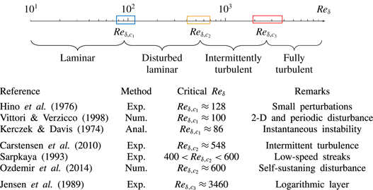
 $Re_{\unicode[STIX]{x1D6FF}}$ is increased, which is illustrated by the diagram in table 1. The transition from laminar to turbulent flow in the Stokes boundary layer has been the topic of extensive theoretical, experimental and numerical studies, due to its close relevance to wave-induced physical processes, such as sediment transport (Traykovski, Wiberg & Geyer Reference Traykovski, Wiberg and Geyer2007) and biological blood flow in an artery (Womersley Reference Womersley1955), and the rich physics associated with the transition process. Apart from the well-known Stokes solution in a laminar boundary layer (Stokes Reference Stokes1851; Lamb Reference Lamb1932), no exact solution exists for the flow in other regimes. Previous studies (Kerczek & Davis Reference Kerczek and Davis1974; Hino, Sawamoto & Takasu Reference Hino, Sawamoto and Takasu1976; Jensen, Sumer & Fredsoe Reference Jensen, Sumer and Fredsoe1989; Akhavan, Kamm & Shapiro Reference Akhavan, Kamm and Shapiro1991a; Sarpkaya Reference Sarpkaya1993; Blondeaux & Vittori Reference Blondeaux and Vittori1994; Vittori & Verzicco Reference Vittori and Verzicco1998; Costamagna, Vittori & Blondeaux Reference Costamagna, Vittori and Blondeaux2003; Carstensen, Sumer & Fredsøe Reference Carstensen, Sumer and Fredsøe2010; Ozdemir, Hsu & Balachandar Reference Ozdemir, Hsu and Balachandar2014) have identified three flow regimes in addition to the laminar flow regime, which include the disturbed laminar regime, the intermittently turbulent regime and the fully turbulent regime, in order of increasing
 $Re_{\unicode[STIX]{x1D6FF}}$.
Diagram of flow regime classifications and selected studies on critical Reynolds numbers.

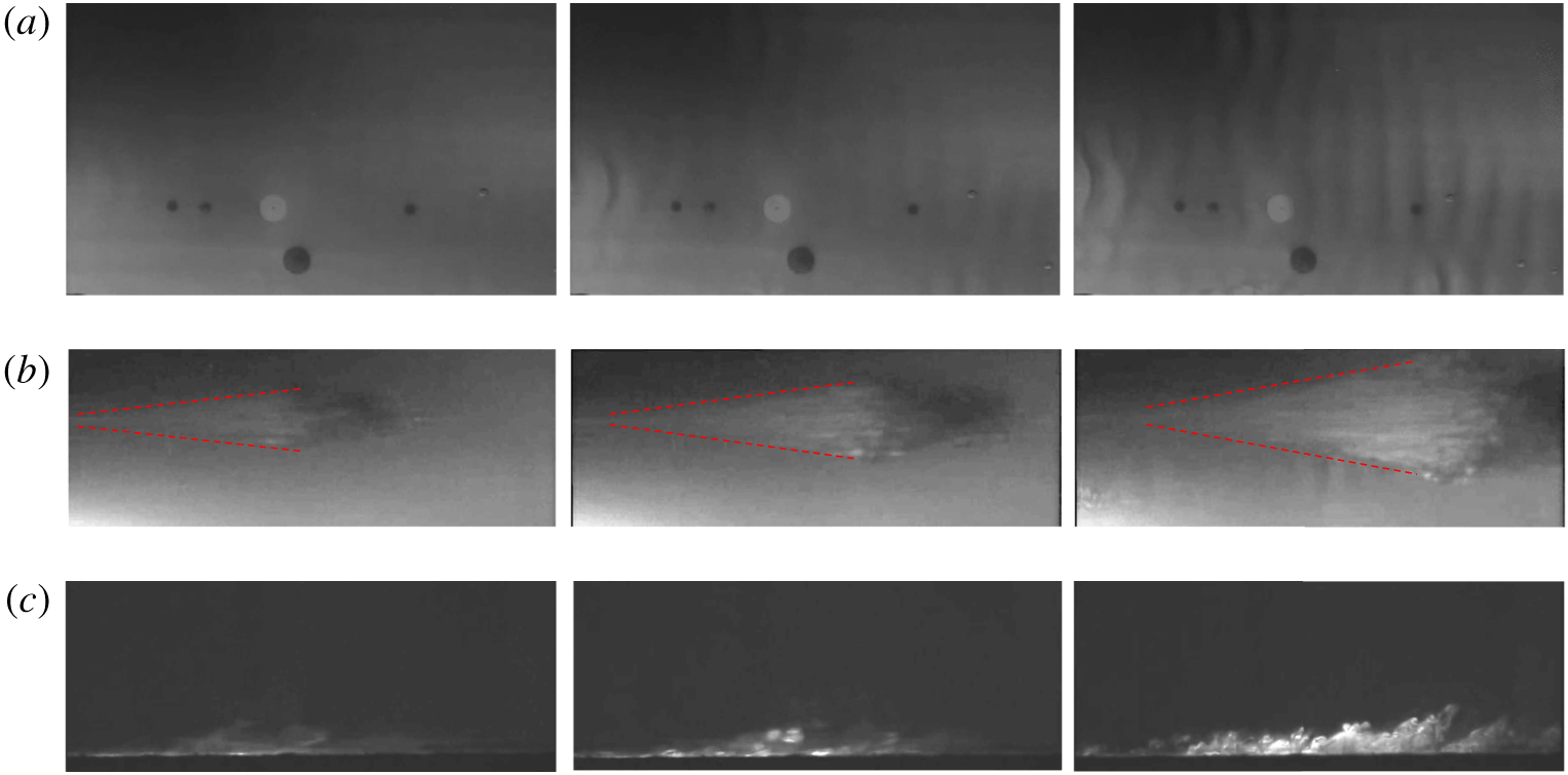
Experimental visualisations of (a) vortex tubes in plan view at  $Re_{\unicode[STIX]{x1D6FF}}=761$ during the phase
 $168^{\circ }<\unicode[STIX]{x1D719}<185^{\circ }$, (b) turbulent spots appearing at isolated arrowhead-shaped areas in plan view as indicated by the dashed lines at
 $Re_{\unicode[STIX]{x1D6FF}}=775$ during the phase
 $130^{\circ }<\unicode[STIX]{x1D719}<169^{\circ }$ and (c) the intensive transverse swirling motion in side view caused by turbulent spots at
 $Re_{\unicode[STIX]{x1D6FF}}=812$. The authors would like to acknowledge professors B. M. Sumer and S. Carstensen for providing the videos.

The disturbed laminar regime is characterised by the appearance of small perturbations to laminar flow as  $Re_{\unicode[STIX]{x1D6FF}}$ is increased beyond
 $Re_{\unicode[STIX]{x1D6FF},c1}\approx 100$ (see table 1). Kerczek & Davis (Reference Kerczek and Davis1974) detected instantaneous growths of instability at
 $Re_{\unicode[STIX]{x1D6FF}}\approx 86$ based on a quasi-static stability analysis. They found that such periodic perturbations are essentially two-dimensional (2-D) and do not significantly affect the velocity profile. The 2-D or quasi-2-D coherent structures emerging at
 $Re_{\unicode[STIX]{x1D6FF}}$ from 374 to 776 are referred to as vortex tubes in Carstensen et al. (Reference Carstensen, Sumer and Fredsøe2010) (figure 1a) and are attributed to an inflection-point instability. The vortex tubes cannot be sustained without appropriate ambient disturbances such as wall imperfections (Scandura Reference Scandura2013). When
 $Re_{\unicode[STIX]{x1D6FF}}$ is increased beyond the second critical value
 $Re_{\unicode[STIX]{x1D6FF},c2}\approx 550$, the flow becomes intermittently turbulent (Carstensen et al. Reference Carstensen, Sumer and Fredsøe2010). Sarpkaya (Reference Sarpkaya1993) observed the evolution of low-speed streaks, characterised by the alternative onset and disappearance of turbulence during the deceleration and acceleration phases of a flow oscillation cycle, respectively. Ozdemir et al. (Reference Ozdemir, Hsu and Balachandar2014) demonstrated that, despite the fact that this flow transition behaviour is self-sustainable from cycle to cycle at
 $Re_{\unicode[STIX]{x1D6FF}}=600$, the transition is considered as incomplete because the velocity profile does not follow the logarithmic law. Carstensen et al. (Reference Carstensen, Sumer and Fredsøe2010) observed the inception of streaks and the subsequent appearance of turbulent spots in isolated areas of arrowhead shapes (figure 1b), leading to intense transverse swirling motion and violent fluctuations of velocity and shear stress (figure 1c).
The formation of turbulent spots in the Stokes boundary layer is analogous to its counterpart observed in steady boundary layer flow, which emerges from finite-length longitudinal streaks that twist, turn and then break down (Robinson Reference Robinson1991; Costamagna et al. Reference Costamagna, Vittori and Blondeaux2003; Mazzuoli, Vittori & Blondeaux Reference Mazzuoli, Vittori and Blondeaux2011). The inception of streaks in the accelerating phase of the flow occurs earlier with increasing  $Re_{\unicode[STIX]{x1D6FF}}$. The reported values of the third critical Reynolds number
 $Re_{\unicode[STIX]{x1D6FF},c3}$ scatter significantly over
 $\mathit{O}(1000)$ in the literature (Hino et al. Reference Hino, Sawamoto and Takasu1976; Jensen et al. Reference Jensen, Sumer and Fredsoe1989; Sarpkaya Reference Sarpkaya1993), primarily because of different criteria used to identify the fully turbulent flow. The occurrence of the fully turbulent flow throughout the entire oscillation cycle has not been observed so far even at very large
 $Re_{\unicode[STIX]{x1D6FF}}$ values. Jensen et al. (Reference Jensen, Sumer and Fredsoe1989) reported that turbulence pervades throughout the major portion of the cycle at
 $Re_{\unicode[STIX]{x1D6FF},c3}=3460$ according to the semi-logarithmic distribution of mean velocity profile, which is a distinctive feature of fully developed turbulent boundary layers.
Linear stability analysis based on instantaneous or global (Floquet) instability theory has been employed to identify  $Re_{\unicode[STIX]{x1D6FF},c2}$ in the literature (Kerczek & Davis Reference Kerczek and Davis1974; Hall Reference Hall1978; Wu Reference Wu1992; Blennerhassett & Bassom Reference Blennerhassett and Bassom2002, Reference Blennerhassett and Bassom2006; Luo & Wu Reference Luo and Wu2010). However, there is a substantial discrepancy in the values of
 $Re_{\unicode[STIX]{x1D6FF},c2}$ obtained from linear instability analysis and experimental observations. The initial attempts with stability analysis failed to discover a growing instability in the finite or infinite Stokes boundary layer within the range of Reynolds number identified by physical experiments (Kerczek & Davis Reference Kerczek and Davis1974; Hall Reference Hall1978). In contrast, the flows seemed to become more stable with increasing
 $Re_{\unicode[STIX]{x1D6FF}}$, according to the results of Floquet stability analysis. This paradox is likely to be caused by the computational constraints at that time to deal with the growing size of the finite-dimensional truncation of the determinant at increasing
 $Re_{\unicode[STIX]{x1D6FF}}$. With the rapid development of computing power, Blennerhassett & Bassom (Reference Blennerhassett and Bassom2002) adopted a similar approach to that by Hall (Reference Hall1978) but successfully detected unstable global modes for
 $Re_{\unicode[STIX]{x1D6FF}}>1416$ as a result. It was demonstrated that the infinitesimal perturbations can arise from base flow defined by the theoretical Stokes boundary layer and then lead to a strong flow nonlinearity through exponential growth at high
 $Re_{\unicode[STIX]{x1D6FF}}$. However, the smallest critical Reynolds numbers for the finite or infinite Stokes boundary layer is still approximately twice the counterpart results determined by experimental studies. We note that the value of
 $Re_{\unicode[STIX]{x1D6FF}}\approx 1416$ identified by Blennerhassett & Bassom (Reference Blennerhassett and Bassom2002) actually represents an upper value of
 $Re_{\unicode[STIX]{x1D6FF},c2}$ beyond which a global instability develops for infinitesimal perturbations, while finite-amplitude disturbances such as the ones induced by wall imperfections inevitably exist in experimental apparatus, which are able to bypass the linear stage and directly trigger the nonlinear instabilities. Luo & Wu (Reference Luo and Wu2010) conducted linear initial value simulations and discovered that an instantaneous growing instability may even alter the mean flow velocity at a much lower value,
 $Re_{\unicode[STIX]{x1D6FF}}\sim 400$, which may be the cause of the discrepancy mentioned above. This finding may explain why Sarpkaya (Reference Sarpkaya1993) observed low-speed streaks at Reynolds number as low as
 $Re_{\unicode[STIX]{x1D6FF}}\approx 400$.
Direct numerical simulations (DNS) of the transition in the Stokes boundary layer have drawn attention to the nonlinear behaviour in the boundary layer and provided a detailed and quantitative description of the turbulence characteristics (e.g. Akhavan, Kamm & Shapiro Reference Akhavan, Kamm and Shapiro1991b; Vittori & Verzicco Reference Vittori and Verzicco1998; Costamagna et al. Reference Costamagna, Vittori and Blondeaux2003; Salon, Armenio & Crise Reference Salon, Armenio and Crise2007; Mazzuoli et al. Reference Mazzuoli, Vittori and Blondeaux2011; Ozdemir et al. Reference Ozdemir, Hsu and Balachandar2014). Wall imperfections are conventionally adopted in DNS to trigger the transition. The predicted velocity fluctuations and wall shear stresses agree well with the experimental values in statistical terms (Akhavan et al. Reference Akhavan, Kamm and Shapiro1991a; Vittori & Verzicco Reference Vittori and Verzicco1998; Costamagna et al. Reference Costamagna, Vittori and Blondeaux2003). The numerical results demonstrated that a streak instability is the dominant mechanism of generating and maintaining turbulence, and the formation of turbulent spots is due to the breakdown of the streaks. Another approach to trigger the transition in DNS is to introduce initial perturbations or background noise. Thomas et al. (Reference Thomas, Blennerhassett, Bassom and Davies2015) suggested that the bypass scenario observed in the transition of the steady flow boundary layer also exists in the Stokes boundary layer. Ozdemir et al. (Reference Ozdemir, Hsu and Balachandar2014) triggered a self-sustaining transitional flow in the Stokes boundary layer at  $Re_{\unicode[STIX]{x1D6FF}}=600$ with finite-amplitude initial perturbations. An astonishing event was observed in which the flow with the largest initial perturbation amplitude recovered to laminar flow within three flow oscillation cycles, whereas the flows with smaller initial perturbation amplitudes remained intermittently turbulent. This observation suggests that sophisticated nonlinear evolution of initial perturbations plays a critical role in the transition process.
Despite the significant progress in understanding the transition process, several questions remain, the following for example. (I) How does the evolution of the vortex tubes affect the onset of turbulent spots? (II) What is the key mechanism for the onset of turbulent spots in the Stokes boundary layer? (III) How do the turbulent spots propagate in the temporal and spatial domains? (IV) How do the turbulent spots remain self-sustained and why are their appearance and decay phase-dependent?
The present study aims to answer these questions through DNS of the Stokes boundary layer. The rest of the paper is organised as follows. In § 2, the mathematical models are introduced. In § 3, the onset of coherent structures and their intrinsic correlation are discussed. The characteristics of the streamwise propagation of turbulent spots are investigated in § 4. Finally, a conceptual model of the self-sustaining mechanism is proposed in § 5. Detailed validations of the numerical model are presented in appendix A.
2 Computational methods
As mentioned at the beginning of § 1, the Stokes boundary layer can be equivalently regarded as the oscillatory motion of a wall or a fluid, which can be treated identically in terms of the numerical formulation via a reference frame conversion. In the present study,  $S$ denotes the reference frame that is fixed to the wall, and
 ${\hat{S}}$ denotes the moving reference frame that is attached to a fluid particle in the free stream. The following relationships hold for
 $S$ and
 ${\hat{S}}$:
 $$\begin{eqnarray}\displaystyle & \displaystyle \hat{x}^{\ast }=x^{\ast }+{\displaystyle \frac{U_{0}^{\ast }}{\unicode[STIX]{x1D70E}^{\ast }}}\cos (\unicode[STIX]{x1D70E}^{\ast }t^{\ast })+C_{0}^{\ast }, & \displaystyle\end{eqnarray}$$
 $$\begin{eqnarray}\displaystyle & \displaystyle \hat{u} ^{\ast }=u^{\ast }-U_{0}^{\ast }\sin (\unicode[STIX]{x1D70E}^{\ast }t^{\ast }), & \displaystyle\end{eqnarray}$$
where  $C_{0}^{\ast }$ denotes the initial position of the fluid particle in the free stream.
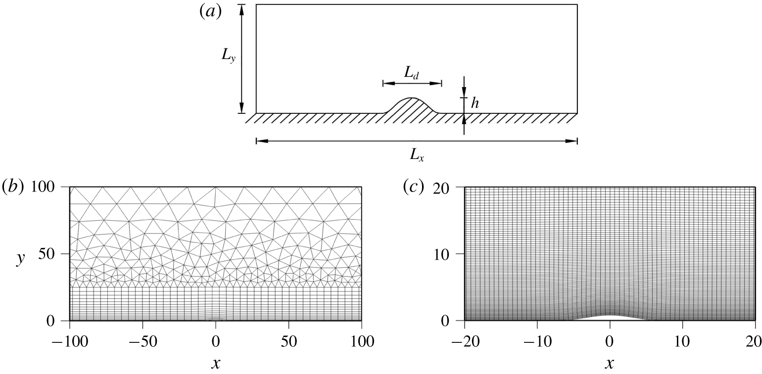
Schematic illustration of the computational domain and the mesh around the roughness element: (a) the computational domain with a smooth hump on the wall, where  $h$ and
 $L_{d}$ denote the height and width of the roughness element, respectively; (b)
 $h$-type mesh around the roughness element; and (c) a close-up view of
 $hp$-refined mesh around the roughness element.

The governing equations for the flow are the non-dimensional incompressible Navier–Stokes (NS) equations and the continuity equation:
 $$\begin{eqnarray}\displaystyle & \displaystyle \frac{\unicode[STIX]{x2202}\boldsymbol{u}}{\unicode[STIX]{x2202}t}+\frac{Re_{\unicode[STIX]{x1D6FF}}}{2}(\boldsymbol{u}\boldsymbol{\cdot }\unicode[STIX]{x1D735})\boldsymbol{u}=-\frac{Re_{\unicode[STIX]{x1D6FF}}}{2}\unicode[STIX]{x1D735}p+\frac{1}{2}\unicode[STIX]{x1D6FB}^{2}\boldsymbol{u}+\boldsymbol{i}_{x}\cos (t), & \displaystyle\end{eqnarray}$$
 $$\begin{eqnarray}\displaystyle & \displaystyle \unicode[STIX]{x1D735}\boldsymbol{\cdot }\boldsymbol{u}=0, & \displaystyle\end{eqnarray}$$
where  $\boldsymbol{u}=(u,v,w)$ is the three-dimensional (3-D) velocity vector corresponding to the
 $x$,
 $y$ and
 $z$ directions, respectively, and
 $p$ is pressure. The last term in (2.3) acts as a harmonic pressure gradient driving the oscillatory flow in the fixed reference frame
 $S$ with
 $\boldsymbol{i}_{x}$ being the unit vector on the
 $x$-axis. The above non-dimensional variables are derived based on:
 $t=t^{\ast }\unicode[STIX]{x1D70E}^{\ast }$,
 $\boldsymbol{x}=\boldsymbol{x}^{\ast }/\unicode[STIX]{x1D6FF}^{\ast }$,
 $\boldsymbol{u}=\boldsymbol{u}^{\ast }/U_{0}^{\ast }$ and
 $p=p^{\ast }/(\unicode[STIX]{x1D70C}^{\ast }(U_{0}^{\ast })^{2})$. The quantity
 $T=2\unicode[STIX]{x03C0}$ is the dimensionless period of the oscillatory flow, and
 $\unicode[STIX]{x1D719}$ denotes the wave phase in degrees; the term
 $t/T$ will hereafter be used to indicate the time instant and the related wave phase can be converted by
 $\unicode[STIX]{x1D719}=(t/T-N)\times 360^{\circ }$, with
 $N$ being the integral number of oscillatory cycle. The vortical flow structure is visualised by employing the instantaneous contours of the vorticity components
 $\unicode[STIX]{x1D74E}=(\unicode[STIX]{x1D714}_{x},\unicode[STIX]{x1D714}_{y},\unicode[STIX]{x1D714}_{z})$ and isosurfaces of
 $Q$ determined by the
 $Q$-criterion (Jeong & Hussain Reference Jeong and Hussain1992), which has been extensively adopted for the identification of an eddy. The eddy is defined in the region by the positive second invariant
 $Q$ of velocity gradient tensor
 $\unicode[STIX]{x1D735}\boldsymbol{u}$. The second invariant
 $Q$ is defined as
 $$\begin{eqnarray}Q={\textstyle \frac{1}{2}}(\Vert \unicode[STIX]{x1D734}\Vert ^{2}-\Vert \boldsymbol{S}\Vert ^{2}),\end{eqnarray}$$
where  $\boldsymbol{S}$ and
 $\unicode[STIX]{x1D734}$ are the symmetric and antisymmetric components of
 $\unicode[STIX]{x1D735}\boldsymbol{u}$, respectively.
The above NS equations are solved by an extensively validated Fourier spectral/ $hp$ element method embedded in Nektar
 $++$ (Cantwell et al. Reference Cantwell, Moxey, Comerford, Bolis, Rocco, Mengaldo, De Grazia, Yakovlev, Lombard and Ekelschot2015), which incorporates the spectral/
 $hp$ element method to discretise the problem in the
 $x$–
 $y$ plane, and a Fourier discretisation is implemented in the
 $z$-direction to resolve the full 3-D features of the flow (Karniadakis Reference Karniadakis1990). Hence, only a 2-D mesh is required in the present study. The 2-D resolution is determined by the distribution of
 $h$-type elements and the interpolant order
 $N_{p}$ for the
 $p$-type refinement, while the spanwise resolution is determined by the Fourier expansion order
 $N_{z}$. In addition, a stabilisation technique called spectral vanishing viscosity (SVV) is employed for the Fourier modes with wavenumbers of the highest 25 % (
 $k_{z}\geqslant 0.75N_{z}$) by increasing the spectral viscosity to enhance the controlled artificial dissipation. The SVV technique has been extensively validated and demonstrated to satisfy the entropy condition and retain spectral accuracy (Cook & Cabot Reference Cook and Cabot2004; Xu & Pasquetti Reference Xu and Pasquetti2004; Kirby & Sherwin Reference Kirby and Sherwin2006). The implicit–explicit (IMEX) time integration method, a velocity correction scheme and a Galerkin formulation are employed for all the simulations. The reader is referred to Bolis (Reference Bolis2013) for more details about this technique and its implementation in Nektar
 $++$.
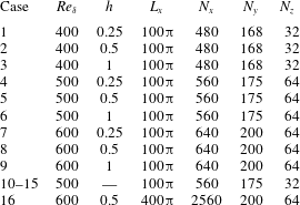
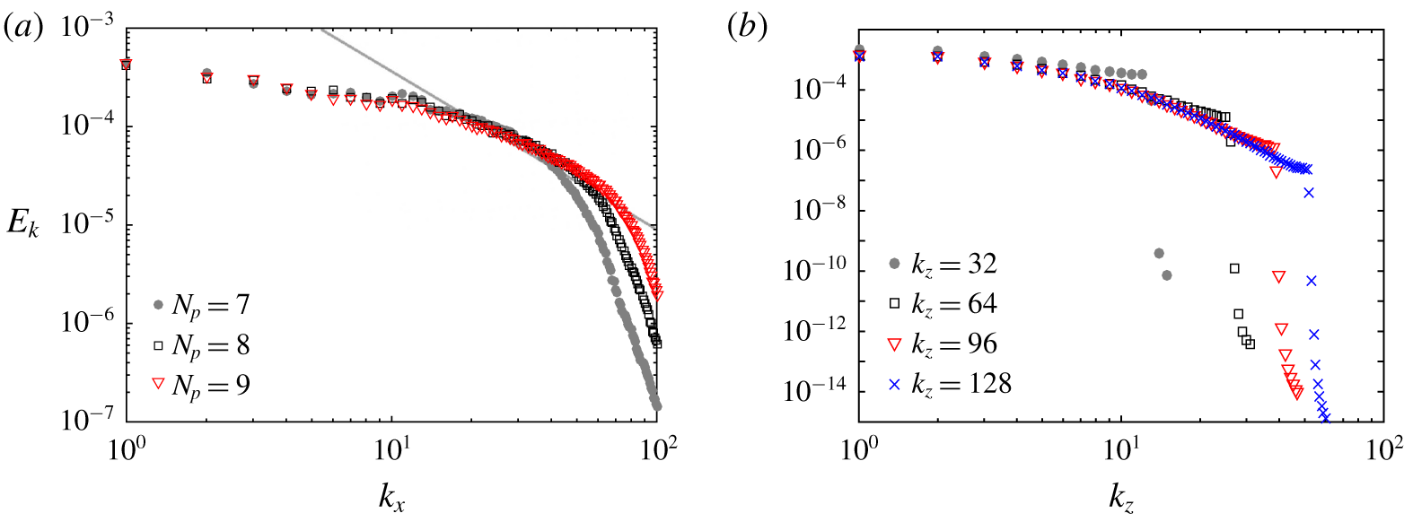
Numerical parameters of the present simulations. Here  $N_{x}$ and
 $N_{y}$ denote the overall resolution along the streamwise and transverse directions of the
 $hp$-refined mesh and
 $N_{z}$ denotes the number of Fourier modes along the spanwise direction. The transverse length and spanwise length are fixed at
 $L_{y}=100$ and
 $L_{z}=32$. The interpolant order
 $N_{p}=6$, 7 and 8 is adopted for simulations at
 $Re_{\unicode[STIX]{x1D6FF}}=400$, 500 and 600, respectively.

A hump is employed as an isolated roughness element to generate the initial perturbations, which avoids artificial assumptions regarding the form of the perturbations and difficulties in tracking the evolution of the isolated flow structures, and is suitable for a study on the bypass transition mechanism (Xu et al. Reference Xu, Sherwin, Hall and Wu2016). As shown in figure 2(a), a hump is temporarily placed on the centre of the wall, the shape function of which is similar to (Xu et al. Reference Xu, Sherwin, Hall and Wu2016)
 $$\begin{eqnarray}f(x)=\left\{\begin{array}{@{}ll@{}}{\displaystyle \frac{h}{2}}(1+\cos (\unicode[STIX]{x1D6FC}x)),\quad & |x-x_{c}|\leqslant {\displaystyle \frac{\unicode[STIX]{x03C0}}{\unicode[STIX]{x1D6FC}}},\\ 0,\quad & |x-x_{c}|>{\displaystyle \frac{\unicode[STIX]{x03C0}}{\unicode[STIX]{x1D6FC}}},\end{array}\right.\end{eqnarray}$$
where  $\unicode[STIX]{x1D6FC}=2\unicode[STIX]{x03C0}/L_{d}$ corresponds to the streamwise wavenumber of the most unstable disturbance and approximately equals 0.36 for
 $400\leqslant Re_{\unicode[STIX]{x1D6FF}}\leqslant 600$ according to Blennerhassett & Bassom (Reference Blennerhassett and Bassom2002). The amplitudes of the hump ranging between 0.125 and 1 are attempted and the results at
 $h=0.25$, 0.5 and 1 are presented for discussion in depth. These results are representative to demonstrate the kinetics of coherent structures and the bypass transition mechanism of the Stokes boundary layer. The boundary layer separation has occurred at
 $h=1$ and the flow instabilities at higher
 $h$ are primarily induced by vortex shedding rather than boundary layer transition. This hump is immediately removed from the wall at cutoff time as soon as the kinetics of the primary vortex tube are independent of its existence. The numerical techniques are detailed in appendix A, including the generation of a mesh with a hump, the mapping approach for removing the hump and a convergence study of the cutoff time.
Table 2 presents the numerical parameters and mesh details of 16 typical cases discussed in the study, which are selected from a database of more extensive numerical results. As noted by Carstensen et al. (Reference Carstensen, Sumer and Fredsøe2010) and Scandura (Reference Scandura2013), a large longitudinal length of the computational domain  $L_{x}$ is required to adequately resolve fully developed vortex tubes and the streamwise propagation of the localised turbulent spots. For this reason,
 $L_{x}$ adopted in most cases is
 $100\unicode[STIX]{x03C0}$, with the height and breadth fixed at 100 and 32, respectively. In addition,
 $L_{x}=400\unicode[STIX]{x03C0}$ is adopted in case 16 at
 $Re_{\unicode[STIX]{x1D6FF}}=600$ to examine the spatial propagation of turbulent spots, which is significantly larger than most of the domain sizes employed in previous 3-D numerical studies (Vittori & Verzicco Reference Vittori and Verzicco1998; Costamagna et al. Reference Costamagna, Vittori and Blondeaux2003; Salon et al. Reference Salon, Armenio and Crise2007; Mazzuoli et al. Reference Mazzuoli, Vittori and Blondeaux2011). The velocity components on the lower and upper boundaries are specified by no-slip and slip boundary conditions, respectively, while a high-order Neumann pressure condition is applied to both boundaries, as described by Blackburn & Henderson (Reference Blackburn and Henderson1999). Periodic conditions are employed for the velocity and pressure components on the streamwise and spanwise boundaries.
The time-step size for each case is carefully chosen to meet the Courant–Friedrichs–Lewy (CFL) stability criterion, which is defined as
 $$\begin{eqnarray}\text{CFL}=\frac{|\boldsymbol{u}|\unicode[STIX]{x0394}t}{\unicode[STIX]{x0394}l},\end{eqnarray}$$
where  $|\boldsymbol{u}|$ is the magnitude of the velocity in a cell and
 $\unicode[STIX]{x0394}l$ is the cell size in the direction of the velocity. The maximum value of the CFL stability criterion is deliberately kept below 0.1 in all the simulations to avoid the possibility of unexpected numerical breakdown. Similar to Xu et al. (Reference Xu, Sherwin, Hall and Wu2016), a hybrid of quadrilateral elements close to the wall and triangular elements in the far-field, as shown in figure 2(b), is adopted in the simulations. The usage of such a mesh configuration is a compromise between accuracy and efficiency. The modified Legendre basis is adopted for both the triangular and quadrilateral elements. A close-up view of the
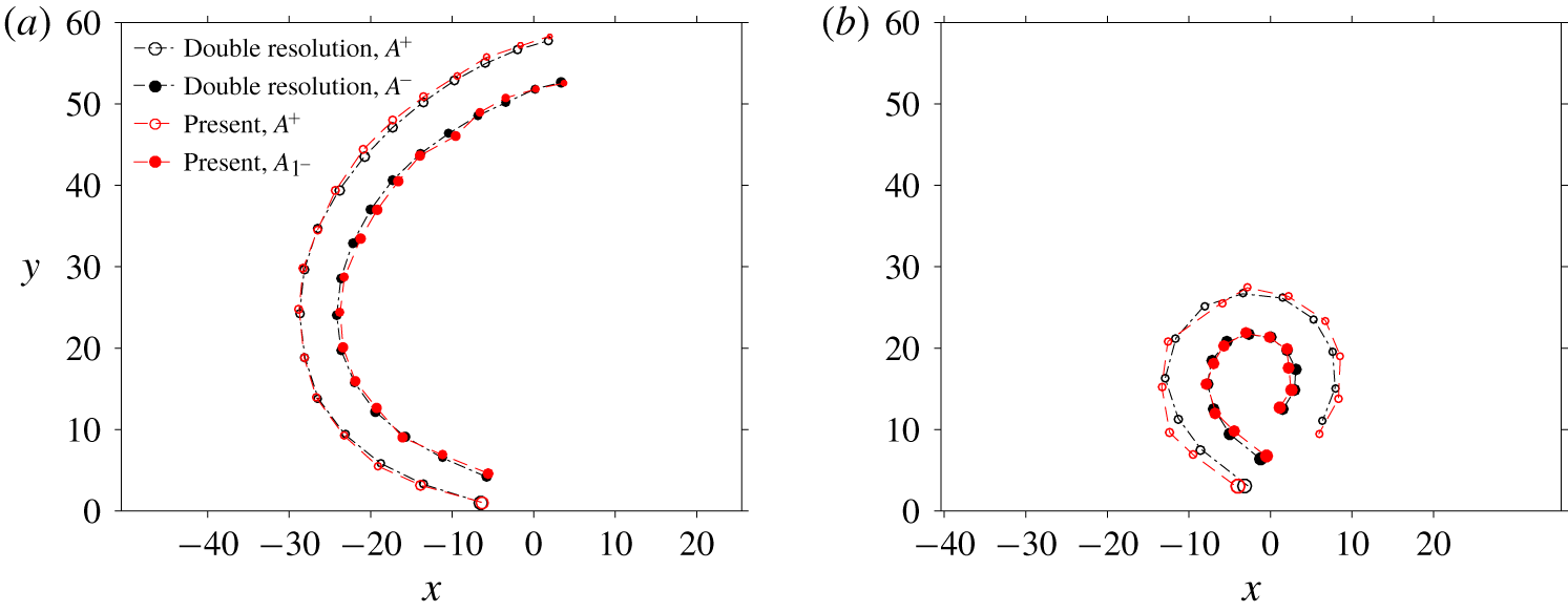
 $hp$ refinement near the bump is shown in figure 2(c). In appendix A, convergence studies are performed to confirm the independence of the results on mesh resolution. The intermediate flow fields at 32 time slices per cycle are employed for flow visualisations and quantitative analysis.
3 The onset of coherent structures
This section investigates the onset mechanism of two types of coherent structures, i.e. vortex tubes and turbulent spots, and their relevance to the transition process of the Stokes boundary layer. Both types of coherent structures have been previously observed in the transitional regime of the Stokes boundary layer (Costamagna et al. Reference Costamagna, Vittori and Blondeaux2003; Carstensen et al. Reference Carstensen, Sumer and Fredsøe2010; Ozdemir et al. Reference Ozdemir, Hsu and Balachandar2014). Although the combination of 2-D finite-amplitude disturbances and 3-D infinitesimal disturbances are suspected to be responsible for the turbulence transition in the boundary layer (Akhavan et al. Reference Akhavan, Kamm and Shapiro1991b), no direct evidence has been obtained so far to demonstrate the linkage between the generation of vortex tubes and turbulent spots.
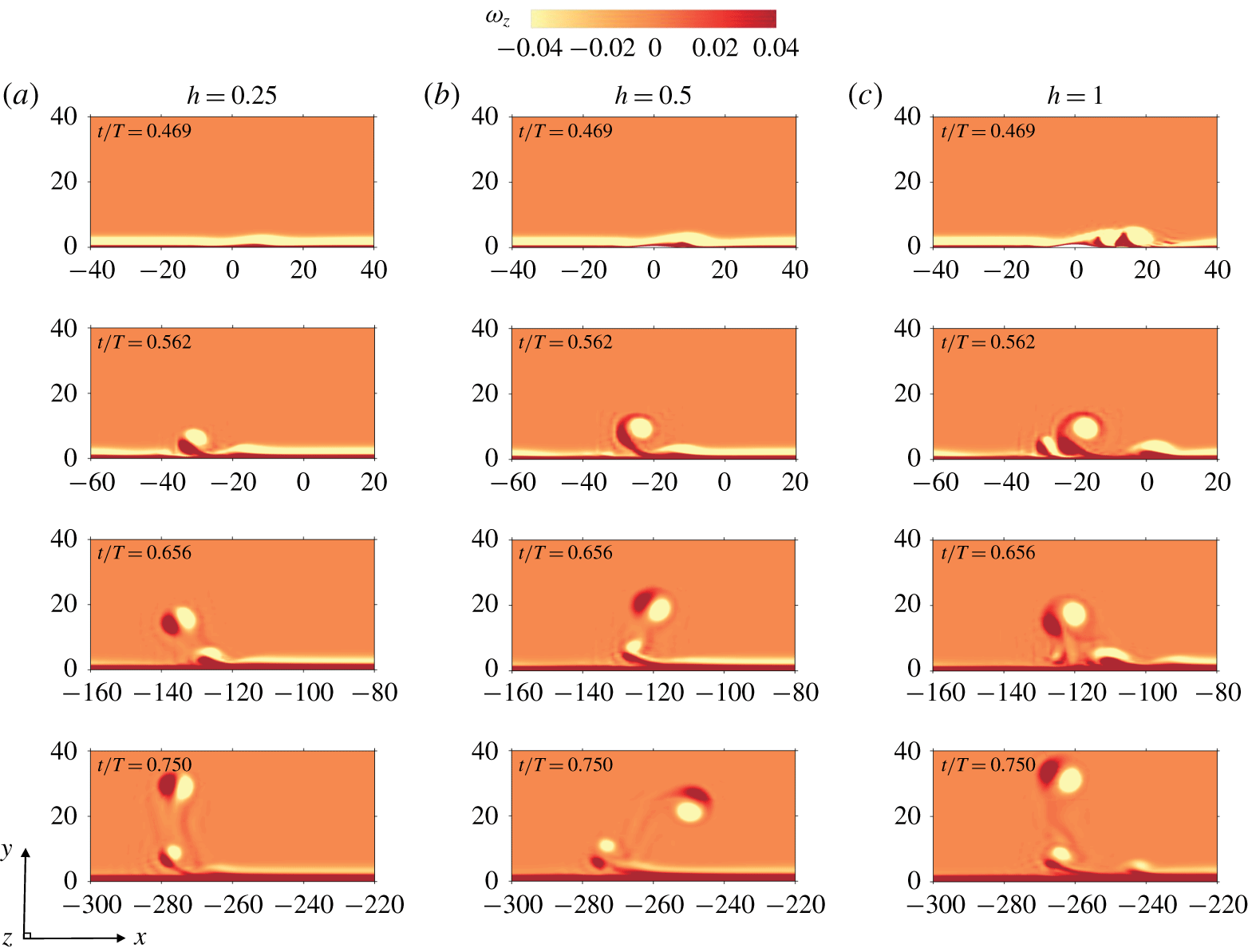
Instantaneous contours of normalised spanwise vorticity  $(\unicode[STIX]{x1D714}_{z})$ at
 $t/T$ showing the onset of vortex tubes triggered by different roughness elements with
 $h=0.25$ (a), 0.5 (b) and 1 (c) located at
 $x=0$ for the flow at
 $Re_{\unicode[STIX]{x1D6FF}}=500$. The temporal roughness element was removed at cutoff time
 $t_{c}/T=17/32\approx 0.531$.

3.1 Vortex tubes
The 2-D flow instability, being triggered by roughness elements of different amplitudes, are first investigated. Figure 3 shows the comparison of the inception and evolution of vortex tubes of cases 4–6 from table 2. The generation process of the vortex tubes is consistent with that observed in previous experimental (Carstensen et al. Reference Carstensen, Sumer and Fredsøe2010) and numerical (Scandura Reference Scandura2013) investigations, despite the differences in the  $Re_{\unicode[STIX]{x1D6FF}}$ values and the progressive manner by which
 $Re_{\unicode[STIX]{x1D6FF}}$ is increased.
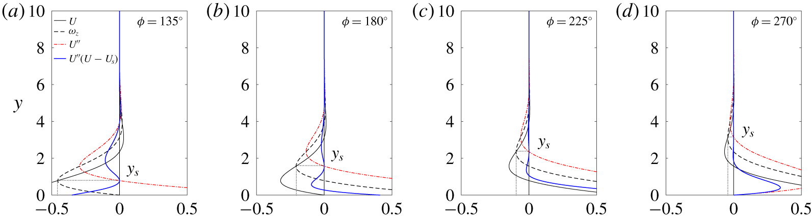
The consensus in the literature is that the Stokes boundary layer is unstable to inflection-point instability (Carstensen et al. Reference Carstensen, Sumer and Fredsøe2010; Scandura Reference Scandura2013; Ozdemir et al. Reference Ozdemir, Hsu and Balachandar2014). According to the classic stability theorem, a necessary condition for the instability of a one-dimensional (1-D) velocity profile  $U(y)$ is the existence of an inflection point
 $y_{s}$ at which
 $U^{\prime \prime }=0$ and
 $U^{\prime \prime }(U-U_{s})\leqslant 0$ for a range of
 $y$, with
 $U^{\prime \prime }(U-U_{s})=0$ only at
 $y=y_{s}$ (Rayleigh Reference Rayleigh1880). The physical explanation is that the perturbed vorticity is mainly advected by the basic flow near the inflection point. In a reference system moving with velocity
 $U_{s}$ at the inflection point
 $y_{s}$, the velocity
 $U-U_{s}$ is positive for
 $y>y_{s}$ and negative for
 $y<y_{s}$. Given that a small sinusoidal vorticity perturbation is located at the inflection point, this velocity profile advects the crest and trough of the perturbation to opposite directions. Thomas et al. (Reference Thomas, Davies, Bassom and Blennerhassett2014) demonstrated that the steepening and amplification of the perturbed vorticity at the inflection point can finally lead to a swirling motion of vortex structures, namely the vortex tube described in the present study.
Illustration of inflection-point instability of the Stokes boundary layer at different phases in the moving reference frame  ${\hat{S}}$, where
 $y_{s}$ denotes the position of the inflection point that satisfies
 $U^{\prime \prime }(y_{s})=0$.

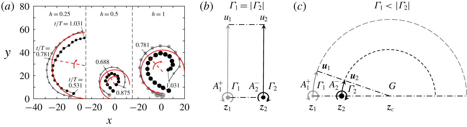
(a) Trace of positive (grey) and negative (black) vortex cores of the primary vortex tubes triggered by three different roughness elements at  $Re_{\unicode[STIX]{x1D6FF}}=500$ (cases 4–6). The theoretical predictions of kinetic motion of two point vortices in an inviscid unbounded fluid are presented in (b) and (c). The applications of the theoretical model are denoted by the red lines in (a), which predict the trajectory (solid), turning radius (dashed) and angular velocity (arrow) of the orbit motion of the vortex pair centre based on the circulations and positions at an instantaneous state in the middle time.

The physical mechanism for the inception and evolution shown in figure 3 is interpreted based on inflection-point instability, as previously described in the literature. The existence of inflection points in the velocity profiles of a laminar Stokes boundary layer at different phases shown in figure 4 is directly responsible for the destabilisation of the negative vortex layer, as indicated in figure 3(a,b) at  $t/T=0.469$. The boundary layer separation and vortex shedding are observed in figure 3(c), possibly due to the large size of roughness element
 $h=1$ that acts like a bluff body attached to the wall (Xiong et al. Reference Xiong, Cheng, Tong and An2018a). The corrugation of the positive vortex layer and the further formation of a counter-rotating vortex pair after the flow reversal, which are observed at
 $t/T=0.562$ in figure 3, resulted from the nonlinear evolution of the inflection-point instability, as suggested by Scandura (Reference Scandura2013). In addition, the onset of the first vortex pair, in turn, caused the phase lag on its right-hand side of the vortex pair, which consequently gave rise to the second vortex pair (at
 $t/T=0.656$), and both vortex pairs left the bottom because of the self-induced velocity (at
 $t/T=0.750$). The coalescence of two adjacent vortex pairs observed at
 $t/T=0.656$ in figure 3(c) was caused by complex interactions between the vortical structures, which were also described in Scandura (Reference Scandura2013).
The kinetics of the vortex tubes after lifting up into the free stream is investigated to facilitate the demonstration of the critical role of vortex tubes on the generation of the secondary instability and bypass transition of the Stokes boundary layer. Although the swirling motion and nonlinear evolution of the vortex tubes have been investigated by Scandura (Reference Scandura2013) and Biau (Reference Biau2016), the mechanism for their full self-induced motion has not been systematically discussed, to the best of the authors’ knowledge. This knowledge gap is possibly due to the prohibitive computational demand to simulate the process, because a large transverse length of the computational domain is required in the simulation to avoid the boundary effect on the top side.
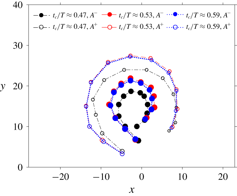
Figure 5(a) shows the position and circulations of the positive and negative vortices of cases 4–6 in the moving frame  ${\hat{S}}$ after their rollup from the boundary. The trajectories of the vortex pair can be potentially determined by the circulations of the vortices based on Helmholtz’s point-vortex equation. According to Stokes’ theorem, the sum and difference of the circulation of a pair of vortices can be calculated by
 $$\begin{eqnarray}\displaystyle & \displaystyle \unicode[STIX]{x1D6E4}_{1}^{+}+\unicode[STIX]{x1D6E4}_{2}^{-}=\int _{A_{1}^{+}}\unicode[STIX]{x1D714}_{z}^{+}\,\text{d}A+\int _{A_{1}^{-}}\unicode[STIX]{x1D714}_{z}^{-}\,\text{d}A=\int _{A}\unicode[STIX]{x1D714}_{z}\,\text{d}A, & \displaystyle\end{eqnarray}$$
 $$\begin{eqnarray}\displaystyle & \displaystyle \unicode[STIX]{x1D6E4}_{1}^{+}-\unicode[STIX]{x1D6E4}_{2}^{-}=\int _{A_{1}^{+}}\unicode[STIX]{x1D714}_{z}^{+}\,\text{d}A+\int _{A_{1}^{-}}|\unicode[STIX]{x1D714}_{z}^{-}|\,\text{d}A=\int _{A}|\unicode[STIX]{x1D714}_{z}|\,\text{d}A, & \displaystyle\end{eqnarray}$$
where  $A_{1}^{+}$ and
 $A_{2}^{-}$ denote the arbitrary shapes of the positive and negative vortices, respectively, while
 $A$ can be a regular integration area, such as a circle or a square, that covers the area of the vortex pair. Therefore, we can easily obtain the circulation of each vortex as
 $$\begin{eqnarray}\unicode[STIX]{x1D6E4}_{i}^{\pm }={\textstyle \frac{1}{2}}\int _{A}(\unicode[STIX]{x1D714}_{z}\pm |\unicode[STIX]{x1D714}_{z}|)\,\text{d}A.\end{eqnarray}$$
Similarly, the position of the vortex, defined as the centre of the vorticity field, is obtained as
 $$\begin{eqnarray}\boldsymbol{z}_{i}=\frac{1}{2\unicode[STIX]{x1D6E4}_{i}^{\pm }}\int _{A}\boldsymbol{z}(\unicode[STIX]{x1D714}_{z}\pm |\unicode[STIX]{x1D714}_{z}|)\,\text{d}A.\end{eqnarray}$$
The pair of vortices for  $h=0.25$ moved along an arc trajectory with an increased turning radius and failed to return to the boundary due to a complete dissipation. In contrast, the vortex tubes of the other two cases turned back to the wall after reaching the peaks of the trajectories in the outer region to form nearly closed trajectory loops. The radius of the trajectory for
 $h=0.5$ is smaller than that for
 $h=1$. The kinetic motion of the vortex pair can be interpreted by a simplified model as shown in figure 5(b,c), which is derived from Helmholtz’s point-vortex equation. Considering two point vortices in an inviscid unbounded fluid, a positive
 $A_{1}^{+}$ with circulation
 $\unicode[STIX]{x1D6E4}_{1}$ at position
 $\boldsymbol{z}_{1}$ and a negative
 $A_{2}^{-}$ with circulation
 $\unicode[STIX]{x1D6E4}_{2}$ at position
 $\boldsymbol{z}_{2}$, the self-induced velocities
 $\boldsymbol{u}_{1}$ and
 $\boldsymbol{u}_{2}$ of these two point vortices can be expressed as
 $$\begin{eqnarray}\displaystyle & \displaystyle u_{1}-\text{i}v_{1}=-\frac{\text{i}}{2\unicode[STIX]{x03C0}}\frac{\unicode[STIX]{x1D6E4}_{2}}{\boldsymbol{z}_{1}-\boldsymbol{z}_{2}}, & \displaystyle\end{eqnarray}$$
 $$\begin{eqnarray}\displaystyle & \displaystyle u_{2}-\text{i}v_{2}=-\frac{\text{i}}{2\unicode[STIX]{x03C0}}\frac{\unicode[STIX]{x1D6E4}_{1}}{\boldsymbol{z}_{1}-\boldsymbol{z}_{2}}, & \displaystyle\end{eqnarray}$$
with the centre  $G$ of the two point-vortex system located at
 $$\begin{eqnarray}\boldsymbol{z}_{c}=\frac{\unicode[STIX]{x1D6E4}_{1}\boldsymbol{z}_{1}+\unicode[STIX]{x1D6E4}_{2}\boldsymbol{z}_{2}}{\unicode[STIX]{x1D6E4}_{1}+\unicode[STIX]{x1D6E4}_{2}}.\end{eqnarray}$$
The above equation suggests that  $\boldsymbol{z}_{c}$ is located on the side closer to the strongest vortex with opposite signs (figure 5c). The orbit motion of the vortex pair is characterised by the angular velocity of
 $\overline{\boldsymbol{z}_{1}\boldsymbol{z}_{2}}$, which is given by
 $$\begin{eqnarray}\unicode[STIX]{x1D6FA}=\frac{\unicode[STIX]{x1D6E4}_{1}+\unicode[STIX]{x1D6E4}_{2}}{2\unicode[STIX]{x03C0}d^{2}},\end{eqnarray}$$
where  $d=|\boldsymbol{z}_{1}-\boldsymbol{z}|$ represents the separation distance between the vortex cores. The turning radius
 $R$, which is defined as the distance from
 $G$ to the centre of
 $\overline{\boldsymbol{z}_{1}\boldsymbol{z}_{2}}$, is determined by
 $$\begin{eqnarray}R=\frac{1}{2}\left|\frac{(\unicode[STIX]{x1D6E4}_{2}-\unicode[STIX]{x1D6E4}_{1})(\boldsymbol{z}_{2}-\boldsymbol{z}_{1})}{\unicode[STIX]{x1D6E4}_{1}+\unicode[STIX]{x1D6E4}_{2}}\right|=\frac{d}{2}\left|\frac{1-\unicode[STIX]{x1D6FE}}{1+\unicode[STIX]{x1D6FE}}\right|,\quad \unicode[STIX]{x1D6FE}=\frac{\unicode[STIX]{x1D6E4}_{1}}{\unicode[STIX]{x1D6E4}_{2}}.\end{eqnarray}$$
Since the separation distance  $d$ is approximately identical for the three cases, the angular velocity of the orbit motion of the vortex pair is mainly dependent on the summation of their circulations, as described by (3.8). If
 $\unicode[STIX]{x1D6FE}=-1$, the vortex pair will move in a straight line perpendicular to
 $\overline{\boldsymbol{z}_{1}\boldsymbol{z}_{2}}$ (figure 5b); for
 $-1<\unicode[STIX]{x1D6FE}<0$, the vortex pair will move along an orbit (figure 5c) and the turning radius decreases with increasing
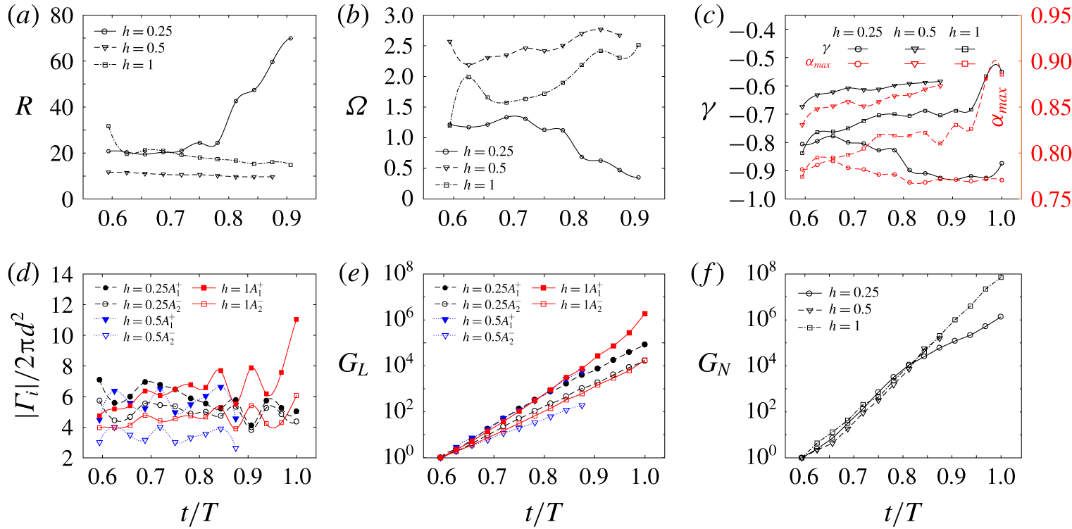
 $\unicode[STIX]{x1D6FE}$ according to (3.9). Trajectories predicted based on (3.9), denoted by the red lines in figure 5(a), agree reasonably with the numerical results despite the influence of the boundary shear layer and the continuous dissipation of the vortices due to the viscous effect. Figure 6(a,b) further quantifies the characteristics of the self-induced motion of the vortex tube for cases 4–6 based on (3.8) and (3.9), indicating the large turning radius
 $R$ and low angular velocity
 $\unicode[STIX]{x1D6FA}$ for
 $h=0.25$ and the opposite scenario for
 $h=0.5$. Some extra numerical tests for different
 $h$ (not shown herein) suggest that no orbit trajectory forms for
 $h\leqslant 0.25$ and the turning radius of the orbit trajectory
 $R$ decreases with increase of roughness height for
 $0.375\leqslant h\leqslant 0.75$. The minimum
 $R$ is reached around
 $h=0.75$ because vortex shedding occurs for higher
 $h$, where complex interactions between multiple vortex tubes are observed before their rollup into the free stream (figure 3c).
The quantitative description of (a) the turning radius  $R$, and (b) angular velocity
 $\unicode[STIX]{x1D6FA}$ according to (3.8) and (3.9) that make use of the instantaneous circulations and positions of the vortex pairs of cases 4–6. (c) The ratio of circulation strength
 $\unicode[STIX]{x1D6FE}=\unicode[STIX]{x1D6E4}_{1}/\unicode[STIX]{x1D6E4}_{2}$ and the corresponding
 $\unicode[STIX]{x1D6FC}_{max}$; (d) the strain field imposed by the other vortex; (e) the overall growth of
 $G_{L}$ by linear prediction of growth rate; and (f) the nonlinear growth of 3-D perturbation energy
 $G_{N}$ integrated from DNS results.

The demonstration of 3-D transition of the vortex tube for the flow at $Re_{\unicode[STIX]{x1D6FF}}=500$ with
 $h=1$ (case 6). (a) Instantaneous isosurface by
 $Q$-criterion at
 $Q=6\times 10^{-3}$ with spanwise vorticity shown in its surface and in the contours of background at
 $z=0$, which are presented in moving reference frame
 ${\hat{S}}$. (b) A close-up view of the evolution of 3-D structure of the vortex pair by top perspective. (c) Dye visualisation of evolution of the Crow instability of two pairs of symmetric counter-rotating vortices generated by towing an outboard triangular flapped wing at velocity
 $U$; reproduced from Bristol et al. (Reference Bristol, Ortega, Marcus and Savas2004). The vortex emanated from the tip side is stronger than that from the flap side. The time shown below was normalised by the time period of the orbit motion, where the angular velocity
 $\unicode[STIX]{x1D6FA}$ was predicted by (3.8).

A sudden drop of the positive vortex for  $h=1$ at
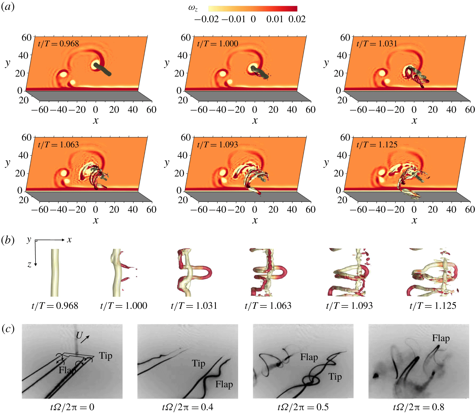
 $t/T\approx 1$, as shown in figure 5(a), is probably induced by the emergence of a new flow instability. The 3-D visualisations of the flow structures presented in figure 7(a) indeed show the 3-D transition of the vortex pair, especially for the positive vortex. Minor waviness of the vortex tube is observed at
 $t/T=0.968$, as shown in figure 7(b). This small waviness was quickly amplified into several ring-like vortices within a short time interval at
 $t/T=1.031$. These phenomena are also similar to the observed deformation of 2-D vortex tubes into 3-D structures reported by Ozdemir et al. (Reference Ozdemir, Hsu and Balachandar2014). Then, the ring-like structure was further stretched, and swept downwards and touched the boundary layer at
 $t/T=1.125$, leading to a complex nonlinear interaction between the free-stream vortex and the Stokes boundary layer. At the same time, the negative vortex remained relatively coherent and stayed in the free stream at a distance far from the wall.
The physical mechanism of the 3-D transition of the vortex tube is interpreted by the Crow instability. Crow (Reference Crow1970) initially investigated the instability of a pair of counter-rotating vortices as a prototype of wingtip vortices behind an aircraft. It was demonstrated that the imposed strain field of each vortex acting on the other leads to the growth of sinusoidal disturbances on the originally straight vortex filaments. The wavelength of the sinusoidal perturbations was several times the separation distance  $d$. The further nonlinear interaction between the instabilities gave rise to the formation of a chain of vortex rings. Bristol et al. (Reference Bristol, Ortega, Marcus and Savas2004) further investigated the instabilities of a pair of counter-rotating vortices with different circulation strengths. The experimental visualisations shown in figure 7(c), reproduced from Bristol et al. (Reference Bristol, Ortega, Marcus and Savas2004), indicate that the amplitude of the sinusoidal disturbances of the weaker vortex has already become much more pronounced than that of the stronger vortex at
 $t\unicode[STIX]{x1D6FA}/2\unicode[STIX]{x03C0}=0.4$. The weaker vortex wrapped around the stronger one at
 $t\unicode[STIX]{x1D6FA}/2\unicode[STIX]{x03C0}=0.5$, which eventually formed periodic vortex rings at
 $t\unicode[STIX]{x1D6FA}/2\unicode[STIX]{x03C0}=0.8$. The above scenarios are qualitatively consistent with the evolution of the vortex tube for case 6 of the present study shown in figure 7(a,b) and they are also hinted at by the supplementary movie 1 of Sumer et al. (Reference Sumer, Jensen, Sørensen, Fredsøe, Liu and Carstensen2010), although it was conducted for solitary waves at a larger Reynolds number.
Following the above qualitative description of the Crow instability, a quantitative analysis of 3-D transition of the vortex tube is demonstrated based on the analytical model proposed by Bristol et al. (Reference Bristol, Ortega, Marcus and Savas2004). The general perturbations of an unbounded vortex pair with different circulation strengths are expressed as Fourier modes  $\hat{\boldsymbol{r}_{i}}=\boldsymbol{r}_{i}\exp (st+\text{i}k_{z}z_{i})$, where
 $\boldsymbol{r}_{i}=(x_{i},y_{i})$ is the eigenvector,
 $k_{z}$ is the spanwise wavenumber and the exponential coefficient
 $s$ for growth of the Crow instability is given by
 $$\begin{eqnarray}s=\unicode[STIX]{x1D6FC}_{max}\times \frac{|\unicode[STIX]{x1D6E4}_{i}|}{2\unicode[STIX]{x03C0}d^{2}}.\end{eqnarray}$$
The maximum eigenvalue  $\unicode[STIX]{x1D6FC}_{max}$ is determined by the equation
 $\unicode[STIX]{x1D6FC}\boldsymbol{r}=\unicode[STIX]{x1D63C}\,\boldsymbol{r}$, where
 $\boldsymbol{r}=(x_{1},y_{1},x_{2},y_{2})$ and the matrix
 $\unicode[STIX]{x1D63C}$ is constituted by four terms that denote the contributions of strain field, mutual induction, orbital rotation and self-induction, for the details of which the reader is referred to Bristol et al. (Reference Bristol, Ortega, Marcus and Savas2004). The results suggested that
 $\unicode[STIX]{x1D6FC}_{max}$ is a function of
 $\unicode[STIX]{x1D6FE}$ and
 $a/d$, with
 $a$ being the vortex radius, but its dependence on
 $\unicode[STIX]{x1D6FE}$ is much more pronounced than
 $a/d$. The values of
 $\unicode[STIX]{x1D6FC}_{max}$ explicitly given in figure 8 of Bristol et al. (Reference Bristol, Ortega, Marcus and Savas2004) are employed in the present study. Therefore, the growth rate of the Crow instability of each vortex of the counter-rotating vortex pair can be quantitatively predicted by (3.10). We note that the linear stability analysis for the Crow instability is no longer valid after significant nonlinear growth of perturbations or the touchdown of the vortex tube and interaction with the boundary layer.
The quantitative results of the Crow instability for cases 4–6 are presented in figure 6(c–f). Figure 6(c) shows the temporal variations of  $\unicode[STIX]{x1D6FC}_{max}$, which are estimated exclusively according to the value of
 $\unicode[STIX]{x1D6FE}$. The interruption of the curves for
 $h=0.5$ at
 $t/T\approx 0.9$ is due to the earlier touchdown of the vortex tube. The instantaneous strength of the strain field of each vortex imposed by the other is demonstrated in figure 6(d), whose values for the positive vortex are always larger than those for the corresponding negative vortex, because the circulation magnitudes of the negative vortex are always stronger than the corresponding positive ones. By employing the values given in figure 6(c,d), the linear prediction of overall temporal growth of the Crow instability can be estimated by
 $$\begin{eqnarray}G_{L}(t_{N})=\mathop{\prod }_{j=1}^{N}\exp [s(t_{j})\unicode[STIX]{x0394}t],\quad N=(t_{N}-t_{0})/\unicode[STIX]{x0394}t,\end{eqnarray}$$
where  $t_{j}=t_{0}+j\unicode[STIX]{x0394}t$ denotes the discrete time and the corresponding time interval is
 $\unicode[STIX]{x0394}t=(1/32)T$. The results shown in figure 6(e) indicate that the largest growth of the Crow instability from
 $t_{0}/T\approx 0.59$ to
 $t_{N}/T=1$ has exceeded
 $10^{6}$ for the positive vortex of case 6 (
 $h=1$). The sinusoidal perturbation of case 6 has already been quite significant at
 $t/T=1$ (figure 7b), after which the linear stability theory may not be applicable at all. The comparison between the growth of the Crow instability of the corresponding positive and negative vortex in figure 6(e) suggests that the 3-D perturbation of the vortex tube is primarily contributed by the weaker vortex of the pair, which is consistent with that of Ozdemir et al. (Reference Ozdemir, Hsu and Balachandar2014). In addition, the exact nonlinear growth of the 3-D perturbation from the DNS results is shown in figure 6(f), which is defined as
 $$\begin{eqnarray}G_{N}(t)=E_{3D}(t)/E_{3D}(t_{0}).\end{eqnarray}$$
The kinetic energy of the 3-D perturbation of the vortex tube  $E_{3D}$ is obtained by
 $$\begin{eqnarray}E_{3D}(t)=\mathop{\sum }_{k_{z}=1}^{N_{z}/2-1}\int _{A}|\hat{\boldsymbol{u}}_{k_{z}}(t)|^{2}\,\text{d}A,\end{eqnarray}$$
where  $\hat{\boldsymbol{u}}_{k_{z}}=\hat{\boldsymbol{u}}_{k_{z}}^{c}+\text{i}\hat{\boldsymbol{u}}_{k_{z}}^{s}$ represents the complex Fourier mode at spanwise wavenumber
 $m$ (Xiong et al. Reference Xiong, Cheng, Tong and An2018b). At
 $t/T=1$, figure 6(f) shows that the overall nonlinear growth of 3-D perturbation of the vortex tube with
 $h=1$ is at least one order larger than that of
 $h=0.25$, which agrees reasonably with the linear prediction of the Crow instability for the positive vortex.
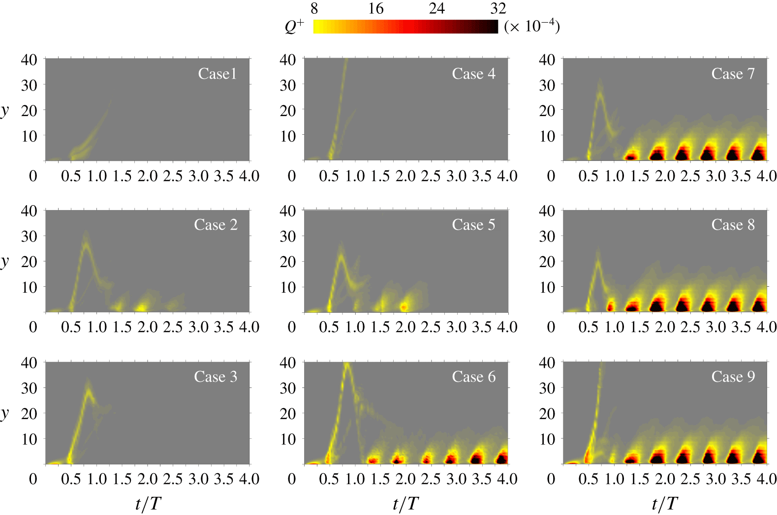
Contour plots of temporal–vertical distribution of  $Q^{+}$ of cases 1–9 in the plane of
 $t/T{-}y$, which are averaged along the streamwise direction after filtering out the negative component by
 $Q^{+}=0.5(Q+|Q|)$.

3.2 Streaks and turbulent spots
The influence of  $Re_{\unicode[STIX]{x1D6FF}}$ and
 $h$ on the dynamics of vortex tubes and their correlation with the emergence of turbulent spots is discussed by examining the contour plots of temporal–vertical distribution of
 $Q$ in the plane of
 $t/T$–
 $y$ of cases 1–9 in figure 8. A parabola-like trajectory emitting from the wall at
 $t/T\approx 0.5$ marks the rollup and orbit motion of the primary vortex tube triggered by the inflection-point instability, while the secondary vortex tubes caused by the nonlinear effect (as shown in figure 3) may also leave an imprint on the contour. On the other hand, the discontinuous contour patches that emerged close to the wall indicate the boundary layer instability, which is similar to the pattern of turbulent spots observed in Ozdemir et al. (Reference Ozdemir, Hsu and Balachandar2014). In general, it is evidenced in figure 8 that the boundary layer transition is highly related to the interaction between the vortex tubes and boundary layer.
Specifically, the width and height of the parabola-like trajectory are associated with the angular velocity  $\unicode[STIX]{x1D6FA}$ and turning radius
 $R$ of the vortex tube, which are quantitatively dependent on the summation and ratio of the circulation strength of positive and negative vortices, as described by (3.8) and (3.9), respectively. It is also seen from the trajectories in figure 8 that the strength of vortex tube coloured by
 $Q^{+}$ increases with increasing
 $h$ and
 $Re_{\unicode[STIX]{x1D6FF}}$. The full orbit motion and touchdown of vortex tubes are observed for all three cases at
 $h=0.5$ (cases 2, 5 and 8) and the increase of
 $Re_{\unicode[STIX]{x1D6FF}}$ leads to an increasing
 $\unicode[STIX]{x1D6FA}$ and a decreasing
 $R$. At
 $Re_{\unicode[STIX]{x1D6FF}}=400$, the vortex tubes for cases 1 and 3 did not return to the boundary so that no boundary layer instability appeared, while the contour patches observed for case 2 indicate the generation of turbulent spots that were not sustained at low Reynolds number. The interruption of the trajectory for case 1 implies that the dissipation of the vortex tube and the scattering components of the trajectory for case 3 were due to the Crow instability, as mentioned in § 3.1. At
 $Re_{\unicode[STIX]{x1D6FF}}=500$, the scenarios of cases 4 and 5 are similar to those of cases 1 and 2, respectively. For case 6, the contour patches emerged after the bifurcation of the trajectory, which was caused by 3-D transition of the primary vortex tube and the touchdown of the ring-like vortices (see figure 7). At
 $Re_{\unicode[STIX]{x1D6FF}}=600$, the contour patches for cases 7–9 indicate that turbulent spots were all sustainable throughout the whole simulation, although the boundary layer instability for case 9 was likely to be triggered by the secondary vortex tube rather than the primary one.
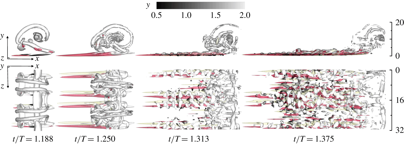
The emerging coherent flow structures at  $Re_{\unicode[STIX]{x1D6FF}}=400$ with
 $h=0.5$ (case 2). The streak is indicated by the isosurfaces of transverse vorticity
 $\unicode[STIX]{x1D714}_{y}$ coloured by yellow (
 $-0.15$) and red (0.15), and the isosurfaces of
 $Q=2.5\times 10^{-3}$ coloured by distance from the wall (
 $y$) indicate the hairpin-like vortex structure and the ring-like vortex swept from the vortex tube.

In order to further investigate the physical mechanism for the above scenarios, the details for the inception of the boundary layer instability for cases 2, 5 and 8 are discussed as follows. The corresponding coherent flow structures of case 2 are visualised in figure 9. The streak structures occurred at an  $Re_{\unicode[STIX]{x1D6FF}}$ value as low as
 $Re_{\unicode[STIX]{x1D6FF}}=400$, although they were not self-sustainable and eventually decayed after one period. In the late acceleration phase, the ring-like vortices that evolved from the sinusoidal positive vortex have already been partially swept downward into the plane boundary layer at
 $t/T=1.188$, as shown in figure 9, similar to the scenario shown in figure 7. The streaks initially stretched out leftwards from the touchdown tips of the ring-like vortices.
The isosurface of the transverse vorticity  $\unicode[STIX]{x1D714}_{y}=\unicode[STIX]{x2202}u/\unicode[STIX]{x2202}z-\unicode[STIX]{x2202}w/\unicode[STIX]{x2202}x$ is adopted to identify the streak structures, which are mainly caused by the fluctuation of the streamwise velocity along the
 $z$-direction. If observed in the moving reference frame
 ${\hat{S}}$, the position of the core of the negative vortex was almost fixed while the streaks move leftwards with the wall due to the viscous effect (
 $t/T=1.250$). The further interaction between the ring-like vortices and boundary layer gave rise to the increased complexity of the flow structures (
 $t/T=1.313$). Along with the elongation and strengthening of the streaks, some hairpin-like vortices that bridged across each pair of streaks can be recognised through the isosurface of
 $Q$ in figure 9. This phenomenon is similar to the observations reported in Ozdemir et al. (Reference Ozdemir, Hsu and Balachandar2014). During the deceleration phase, when the flow was under an adverse pressure gradient, the streaks twisted and lost regularity, while the hairpin vortices rolled with fast transient growth of their strength (
 $t/T=1.375$). In contrast, the coherence of the free-stream vortices decreased after mixing with the boundary layer. The burst of turbulence featured by the breakdown of the streak and hairpin structures leads to the turbulent spots that are observed and discussed in the present study and numerous studies in the literature (e.g. Sarpkaya Reference Sarpkaya1993; Brandt, Schlatter & Dan Reference Brandt, Schlatter and Dan2004; Ozdemir, Hsu & Balachandar Reference Ozdemir, Hsu and Balachandar2013; Ozdemir et al. Reference Ozdemir, Hsu and Balachandar2014; McKeon Reference McKeon2017; Jiménez Reference Jiménez2018).
Interaction between quasi-2-D vortex tube and the Stokes boundary layer otherwise at laminar state at  $Re_{\unicode[STIX]{x1D6FF}}=500$ with
 $h=0.5$ (case 5). The instantaneous isosurfaces show
 $Q=6\times 10^{-3}$ with spanwise vorticity
 $\unicode[STIX]{x1D714}_{z}$ shown in its surface and in the background at
 $z=0$. The reference system is
 ${\hat{S}}$.

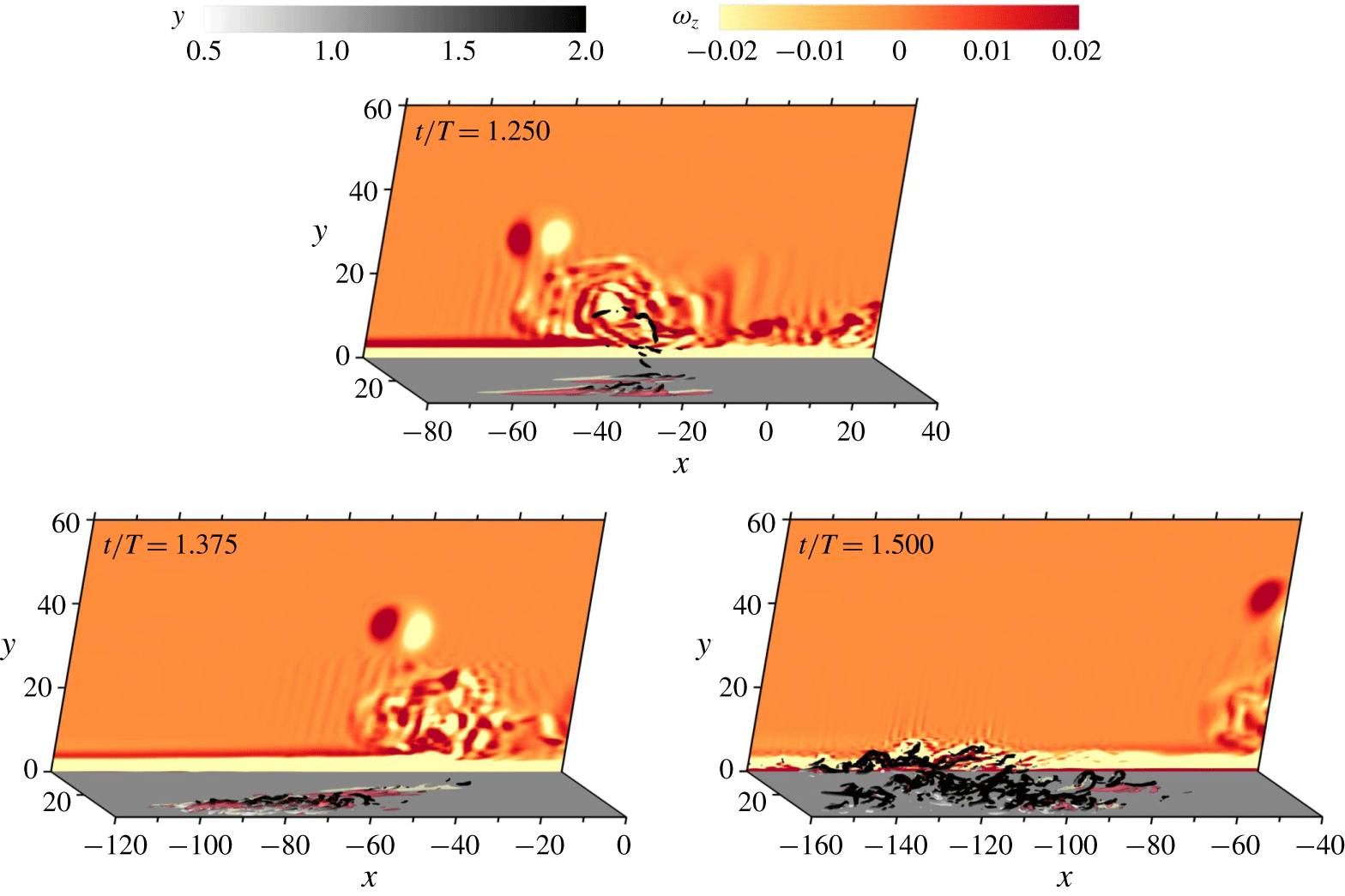
The occurrence of turbulent spots for case 5 was generated without direct interaction with the ring-like vortex as described above. As shown in figure 10, no significant coherent streaks are observed along with the boundary layer after a direct touchdown of a quasi-2-D vortex tube, and figure 8 also indicates that case 5 has not experienced significant growth of boundary instability around  $t/T=1$. Instead, the onset of streaks and hairpin vortices were triggered in the subsequent deceleration phase during
 $t/T=1.25{-}1.5$ by the scattering free-stream vortices that evolved from the original coherent vortex tube, which are indicated by the
 $\unicode[STIX]{x1D714}_{z}$ contours shown in figure 11.
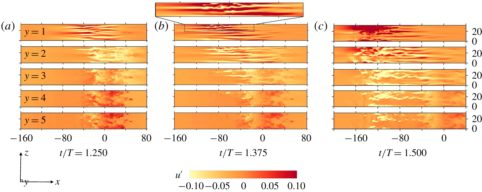
The streak breakdown and ejection of hairpin vortices at the end of the deceleration phase ( $t/T=1.500$) are demonstrated with an isosurface of
 $Q$ coloured by the distance from the wall. The contours of the streamwise fluctuation velocity
 $u^{\prime }$ of
 $x{-}z$ slices at different distances from the wall are presented in figure 12 to obtain a better physical understanding of the transition process. At
 $t/T=1.250$, the inception of the streaks occurred at
 $y=1$, while disturbances without obvious structures are observed in the flow field for
 $y\geqslant 2$. The amplitude of
 $u^{\prime }$ increased as the flow further decelerated. The interaction between streaks of different
 $u^{\prime }$ values caused twisting and turning of the streaks, which can be seen from the slices at
 $y=1$ and 2 at
 $t/T=1.375$. At
 $t/T=1.500$, the flow structures broke down and split into short segments at
 $t/T=1.250$, leading to a burst of turbulent spots close to the wall and an ejection of turbulent spots into the free stream to an elevation of at least
 $y=5$. The above observations qualitatively agree with independent numerical (Costamagna et al. Reference Costamagna, Vittori and Blondeaux2003; Mazzuoli et al. Reference Mazzuoli, Vittori and Blondeaux2011) and experimental (Sarpkaya Reference Sarpkaya1993) observations.
Formation of streaks, rollup of hairpin vortices, their breakup and ejection into free stream following figure 10 (case 5) in subsequent deceleration phase. The streak is indicated by the isosurfaces of transverse vorticity  $\unicode[STIX]{x1D714}_{y}$ coloured by bright yellow (
 $-0.2$) and red (0.2), and the isosurfaces of
 $Q=8\times 10^{-3}$ coloured
 $y$ indicate the hairpin-like vortex structure and turbulent spots. The reference system is
 ${\hat{S}}$.

The slice contours of streamwise velocity fluctuation  $u^{\prime }=u-U(y,t)$ at different heights from
 $y=1$ (top) to 5 (bottom) of figure 11 (case 5) with an interval of 1 in the
 $x{-}z$ plane, where
 $U(y,t)$ denotes the theoretical solution of the Stokes boundary layer. The close-up view of (b) indicates the spatial twist and fluctuation of streaks.

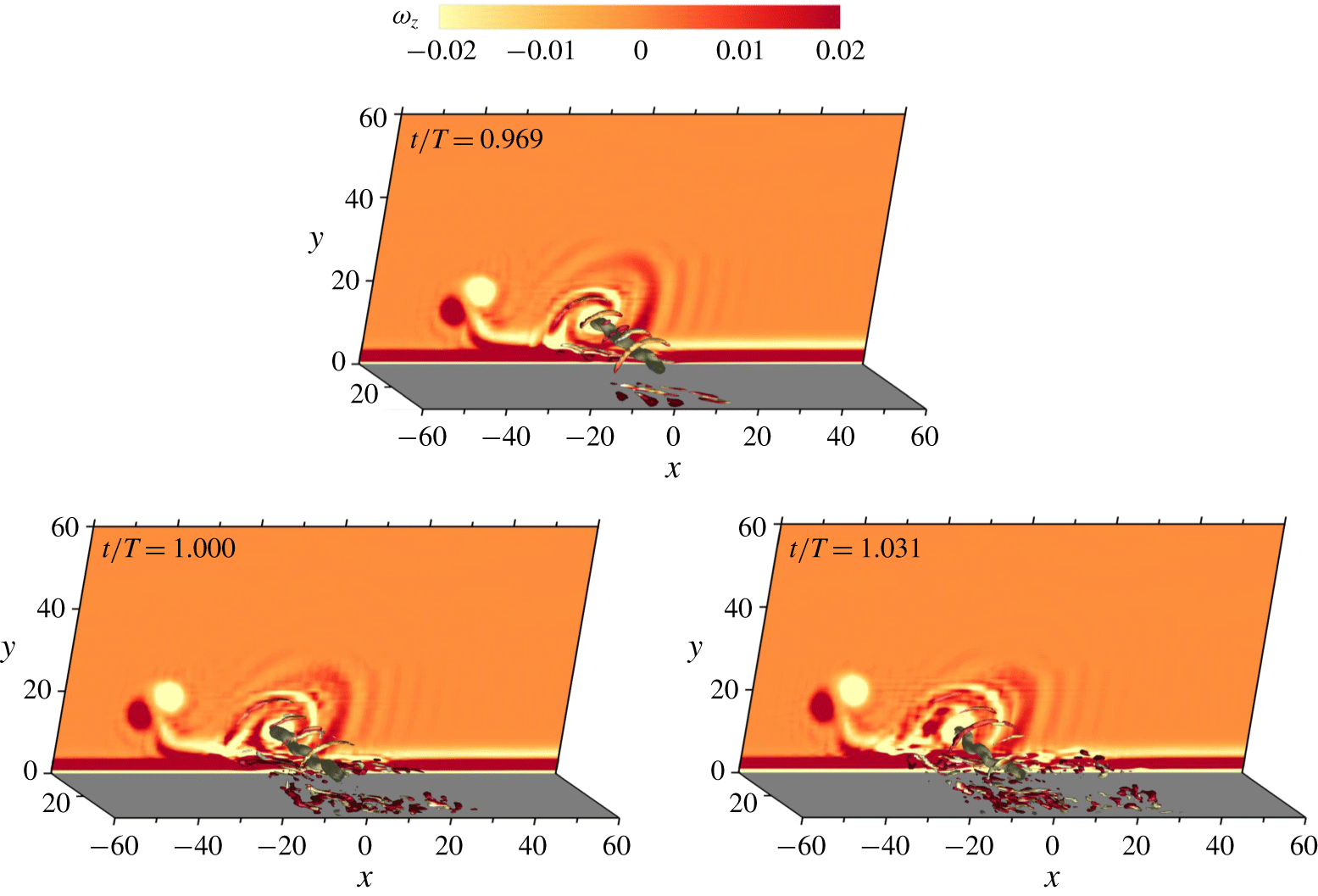
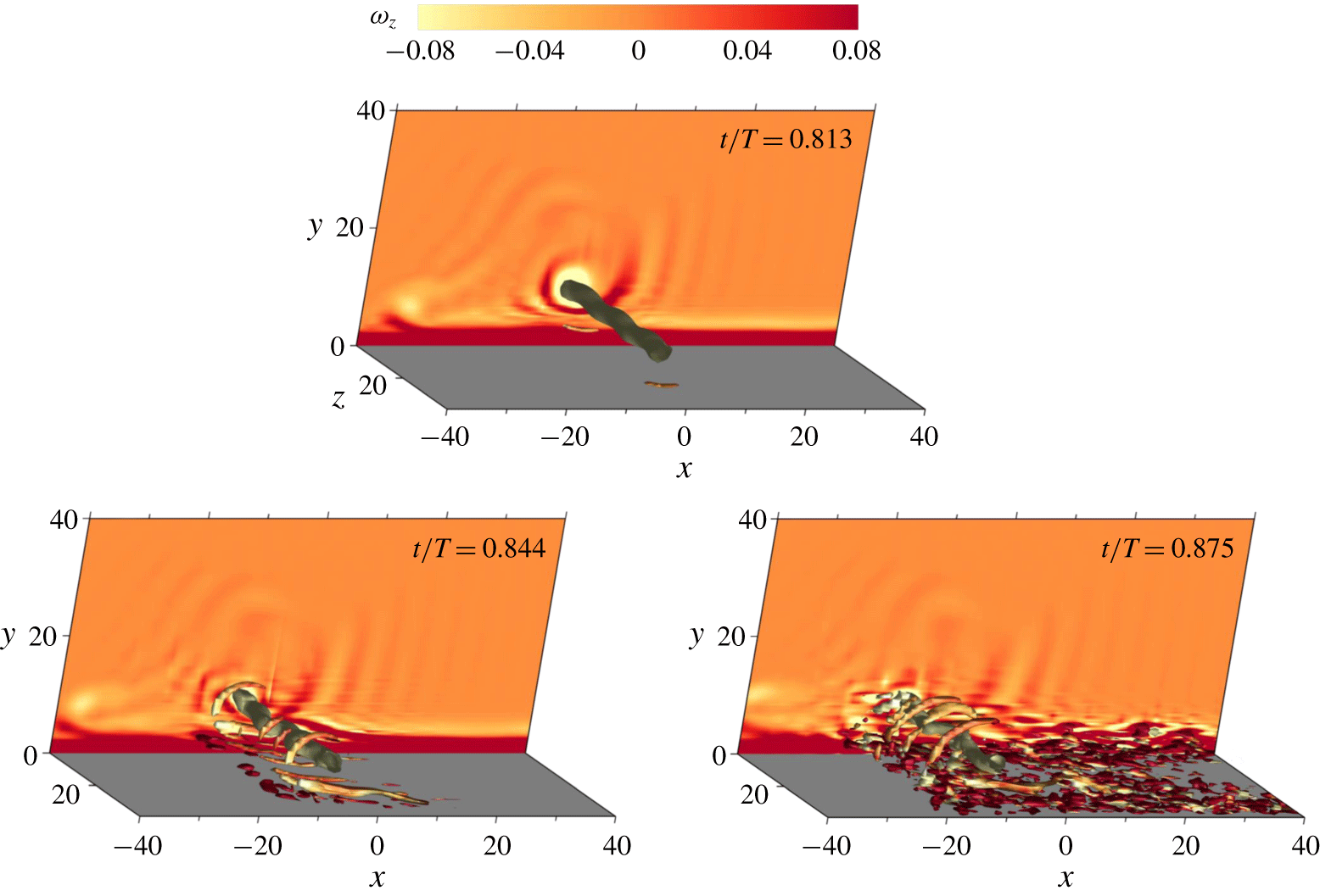
For case 8, a quasi-2-D vortex tube directly induced significant boundary layer instabilities. As shown in figure 13, the streaks and turbulent spots grew rapidly after touchdown of the vortex tube at  $t/T\approx 0.8$. Only a slight waviness of the vortex tube developed at this instant since the fast orbit motion had limited the overall growth of the Crow instability of the vortex tube in the free stream. It is also noted that the transition occurred during the deceleration phase of
 $t/T=0.750{-}1.000$, half a period earlier than for cases 2 and 5.
Instantaneous flow structures for  $h=0.5$ at
 $Re_{\unicode[STIX]{x1D6FF}}=600$ (case 8), which are visualised by isosurface of
 $Q=8\times 10^{-3}$ and
 $4\times 10^{-3}$ coloured by spanwise vorticity
 $\unicode[STIX]{x1D714}_{z}$ with the background showing the contour of
 $\unicode[STIX]{x1D714}_{z}$ at
 $z=0$. The reference system is
 ${\hat{S}}$.

To reveal the fundamental bypass transition mechanisms of the scenarios demonstrated above, a simplified numerical model is established by considering an initial boundary value problem where an artificial vortex disturbance is directly introduced into the Stokes boundary layer. The artificial vortex disturbance has the form of an Oseen–Lamb vortex, the velocity field of which in an unbounded field can be analytically expressed as
 $$\begin{eqnarray}\tilde{\boldsymbol{u}}(\unicode[STIX]{x1D6E4}_{0},\boldsymbol{r},\boldsymbol{r}_{0})=\frac{\unicode[STIX]{x1D6E4}_{0}}{2\unicode[STIX]{x03C0}(\boldsymbol{r}-\boldsymbol{r}_{0})^{2}}\left\{1-\exp \left[-\frac{(\boldsymbol{r}-\boldsymbol{r}_{0})^{2}}{4\unicode[STIX]{x1D708}t_{0}}\right]\right\}(\boldsymbol{r}-\boldsymbol{r}_{0}),\end{eqnarray}$$
which has an initial circulation  $\unicode[STIX]{x1D6E4}_{0}$ and radius
 $\unicode[STIX]{x1D70E}_{0}=\sqrt{4\unicode[STIX]{x1D708}t_{0}}$ located at
 $\boldsymbol{r}_{0}$. Since the vortex disturbance is placed above a wall, its overall expression in a semi-infinite field should consider the contribution from a mirror counterpart:
 $$\begin{eqnarray}\boldsymbol{u}(\boldsymbol{r})=\tilde{\boldsymbol{u}}(\unicode[STIX]{x1D6E4}_{0},\boldsymbol{r},\boldsymbol{r}_{0})+\tilde{\boldsymbol{u}}(-\unicode[STIX]{x1D6E4}_{0},\boldsymbol{r},\boldsymbol{r}_{1}),\end{eqnarray}$$
where  $\boldsymbol{r}_{0}=(x_{0},y_{0},z_{0})$ and
 $\boldsymbol{r}_{1}=(x_{0},-y_{0},z_{0})$ are symmetric with respect to the
 $x$-axis. In addition to a purely 2-D Oseen–Lamb vortex, a sinusoidal perturbation along the spanwise direction is introduced to mimic the influence of the Crow instability, which can be expressed by
 $$\begin{eqnarray}x_{0}(z_{0})=x_{c}+A_{z}\sin \left(\frac{2\unicode[STIX]{x03C0}k_{z}}{L_{z}}z_{0}\right).\end{eqnarray}$$
Six different simulations (cases 10–15) are carried out to investigate the influence of three factors, including the vertical position where the vortex is imposed, the spanwise rotating direction of the vortex and sinusoidal perturbation. The spanwise amplitude and wavenumber for the vortex with the sinusoidal perturbation are set as  $A_{z}=0.5$ and
 $k_{z}=3$, respectively. The other parameters determined with reference to the vortex naturally generated by the inflection-point instability are
 $\unicode[STIX]{x1D6E4}_{0}=\pm 0.25$ and
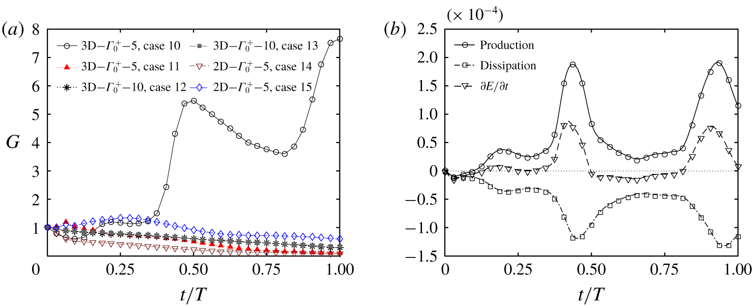
 $\unicode[STIX]{x1D70E}_{0}=1.5$. The overall growth of the kinetic energy of the perturbation field
 $G=E(t)/E(0)$ is summarised in figure 14(a), where the kinetic energy of the perturbation field is obtained by
 $E=0.5\int _{V}(u^{\prime 2}+v^{\prime 2})\,\text{d}V$. The parameter set-ups of cases 10–15 are symbolised by the figure legend A–B–C, where A denotes the vortex disturbance with or without 3-D sinusoidal disturbance, B represents the sign of the spanwise circulation and C indicates the initial vertical position of the vortex disturbance.
(a) Comparison of transient growth  $G$ of total disturbance energy
 $E$ after imposing a localised artificial perturbation of different forms or at different vertical positions into theoretical Stokes boundary layer. (b) Production, dissipation and overall growth rate of disturbance energy determined from Reynolds–Orr equation.

Among the six cases simulated, a significant growth of the perturbation is only observed in case 10, where a positive vortex disturbance with sinusoidal perturbation was placed at  $y=5$. The perturbations located at
 $y=10$ were too far away from the wall to affect the boundary layer so that the perturbation energy of cases 12 and 13 dissipated almost linearly in time. For cases 11 and 15, the formation of a vortex pair by the interaction of the negative vortex disturbance and the positive shear layer led to the initial increase of
 $G$, followed by a gradual decay in one flow period after the rollup of the vortex pair. The quicker dissipation observed for case 11 is due to the 3-D effect. The comparison between the results of cases 10 and 14 suggests that the sinusoidal perturbation of the vortex disturbance plays a critical role in triggering the boundary layer instability. Specifically, the disturbance energy in case 14 monotonically decayed during the whole cycle, whereas the disturbance energy in case 10 recovered quickly after the initial decrease and experienced explosive transient growth during the late stage of the deceleration phase
 $0.375<t/T<0.5$, which is featured by the emergence of streaks and turbulent spots similar to figure 13 but towards opposite
 $x$ directions. In conclusion, the effect of the vortex disturbance on transition of the Stokes boundary layer is dependent on its location, sign and the existence of sinusoidal perturbation.
The turbulent energy balance of case 10 is quantified by the well-known Reynolds–Orr equation (Schlichting Reference Schlichting1979):
 $$\begin{eqnarray}\frac{\unicode[STIX]{x2202}E}{\unicode[STIX]{x2202}t}=-\int _{V}u_{i}^{\prime }u_{j}^{\prime }\frac{\unicode[STIX]{x2202}U_{i}}{x_{j}}\,\text{d}V-\frac{1}{Re_{\unicode[STIX]{x1D6FF}}}\int _{V}\frac{\unicode[STIX]{x2202}u_{i}^{\prime }}{\unicode[STIX]{x2202}x_{j}}\frac{\unicode[STIX]{x2202}u_{i}^{\prime }}{\unicode[STIX]{x2202}x_{j}}\,\text{d}V\quad (i,j=1,2,3),\end{eqnarray}$$
where  $U_{i}$ represents the components of mean velocity and
 $u_{i}^{\prime }=u_{i}-U_{i}$ represents the disturbance components. The results shown in figure 14(b) indicate that
 $\unicode[STIX]{x2202}E/\unicode[STIX]{x2202}t$ became positive from
 $t/T\approx 0.1$, but it peaked at
 $t/T\approx 0.4$ when the production term was significantly larger than the dissipation term, indicating the fast evolution of the disturbance in the late deceleration phase. Subsequently, the disturbance energy decreased in the next acceleration phase for
 $\unicode[STIX]{x2202}E/\unicode[STIX]{x2202}t$ being negative, and then the variation pattern repeated in general.
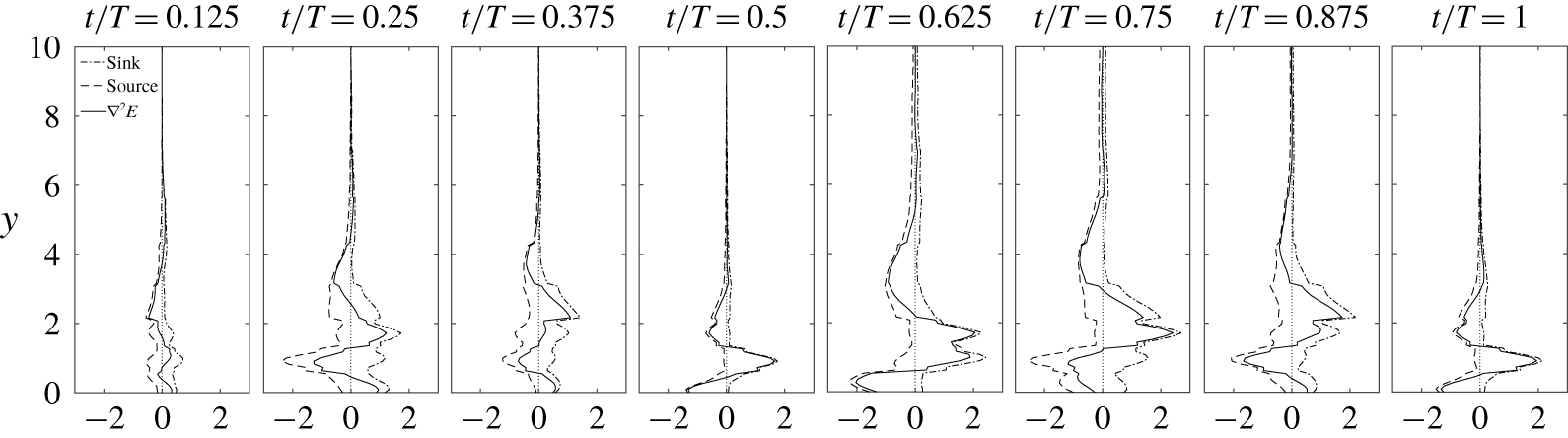
The instantaneous vertical distribution of sink (positive component), source (negative component) and overall evolution of disturbance energy of case 10.

To analyse the spatial distribution of the sink and source that contribute to the dissipation and production of the disturbance energy within the boundary layer, an equation derived from the rotational form of the NS equation is adopted:
 $$\begin{eqnarray}\unicode[STIX]{x1D6FB}^{2}E=2\unicode[STIX]{x1D74E}_{m}\boldsymbol{\cdot }\unicode[STIX]{x1D74E}_{d}+\unicode[STIX]{x1D74E}_{d}\boldsymbol{\cdot }\unicode[STIX]{x1D74E}_{d}-\boldsymbol{u}_{m}\boldsymbol{\cdot }\unicode[STIX]{x1D735}\times \unicode[STIX]{x1D74E}_{d}-\boldsymbol{u}_{d}\boldsymbol{\cdot }\unicode[STIX]{x1D735}\times \unicode[STIX]{x1D74E}_{m}-\boldsymbol{u}_{d}\boldsymbol{\cdot }\unicode[STIX]{x1D735}\times \unicode[STIX]{x1D74E}_{d},\end{eqnarray}$$
where  $\boldsymbol{u}$ and
 $\unicode[STIX]{x1D74E}$ represent the velocity and vorticity fields, respectively, and the subscripts
 $m$ and
 $d$ represent the mean flow and disturbance flow, respectively. A similar approach was applied by Sengupta, De & Sarkar (Reference Sengupta, De and Sarkar2003), Sengupta & Dipankar (Reference Sengupta and Dipankar2005) and Dipankar, Sengupta & Talla (Reference Dipankar, Sengupta and Talla2007) to investigate the boundary layer transition. Figure 15 shows the vertical distribution of the disturbance energy sources and sinks, which is estimated by the integration of the negative and positive components of the right-hand side of (3.18) over the
 $x{-}z$ plane at different
 $y$-positions, respectively. The peak of the source initially achieved a maximum amplitude at the start of the deceleration phase
 $t/T=0.25$ at position
 $y\approx 1$, which is likely to be associated with the onset of streaks. Then the primary peak of the source moved upwards to
 $y\approx 4$ at
 $t/T=0.875$ and finally disappeared at
 $t/T=1$. On the other hand, the new peak of the source attached to the wall occurred at
 $t/T=0.5$, when a sharp peak of the sink is also observed at
 $y\approx 1$. The distribution of
 $\unicode[STIX]{x1D6FB}^{2}E$ for
 $1<y<3$ was dominated by the sink in the subsequent acceleration phase, which is responsible for the disappearance of the turbulent spots that lifted up from the near-wall region. The profiles of the sink, source and overall evolution of the disturbance energy at
 $t/T=1$ are almost repetitions of those at
 $t/T=0.5$, implying a certain feedback mechanism between the dissipation and production of disturbance energy, which will be further classified in § 5.
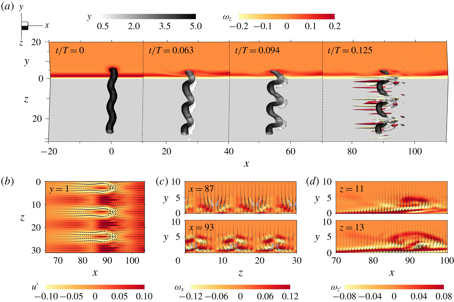
(a) Interaction between the Oseen–Lamb vortex with sinusoidal perturbation and the Stokes boundary layer (case 10). The snapshots are observed in the fixed reference frame  $S$. The instantaneous isosurfaces show
 $Q=4.8\times 10^{-3}$ coloured by
 $y$ with
 $\unicode[STIX]{x1D714}_{z}$ shown in the background at
 $z=0$. The streaks that emerge at
 $t/T=0.125$ are indicated by the isosurfaces of transverse vorticity
 $\unicode[STIX]{x1D714}_{y}$ by bright yellow (
 $-0.12$) and red (0.12). (b) The contour of streamwise velocity fluctuation
 $u^{\prime }$ and vector by (
 $u^{\prime },w^{\prime }$) at
 $y=1$, (c) the contour of streamwise vorticity and vector by (
 $w^{\prime },v^{\prime }$) at
 $x=87$ and 93 with arrows indicating the sweeping-down and lifting-up motion, and (d) the contour of spanwise vorticity of perturbation field
 $\unicode[STIX]{x1D714}_{z}^{\prime }$ and vector by (
 $u^{\prime },v^{\prime }$) at
 $z=11$ and 13.

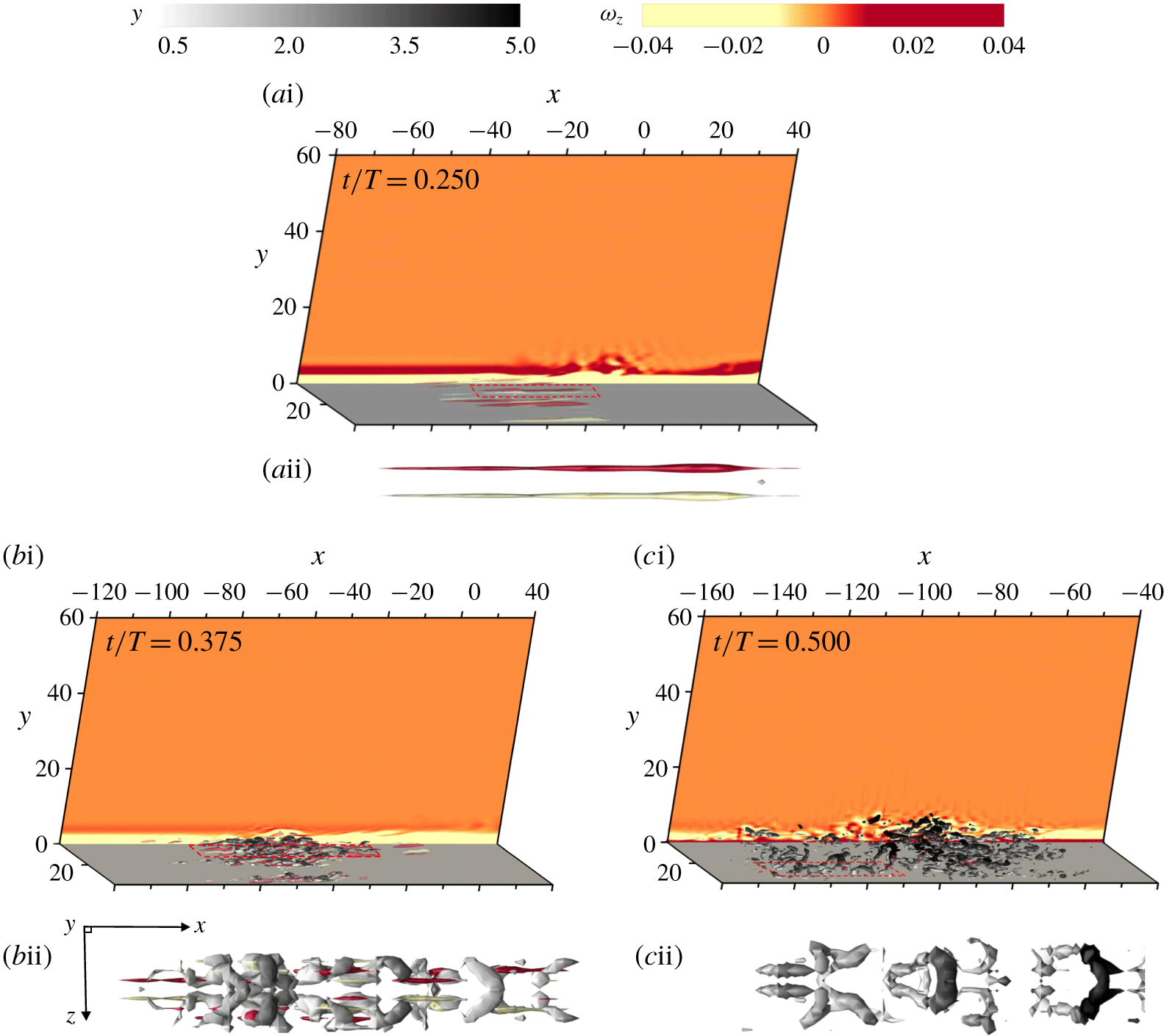
(ai,bi,ci) Flow visualisations observed in reference system  ${\hat{S}}$ present the further development of streaks and hairpin vortices following figure 16 (case 10). (aii,bii,cii) The corresponding close-up top views demonstrate the flow structures in the denoted regions. The isosurfaces of transverse vorticity
 $\unicode[STIX]{x1D714}_{y}$ are coloured by bright yellow (
 $-0.2$) and red (0.2), and the isosurfaces of
 $Q=8\times 10^{-3}$ are coloured by
 $y$.

The corresponding flow structures of case 10 are displayed in figure 16(a) to examine the initial physical process for receptivity of a 3-D free-stream vortex perturbation and growth of boundary layer instability. At  $t/T=0.063$, the interaction with the shear layer first led to the fast amplification of the sinusoidal disturbance of the vortex and change of its inclination angle relative to the wall. Meanwhile, the corresponding near-wall disturbances were induced below the touchdown points of the distorted vortex. The near-wall disturbances quickly grew into hairpin vortices with an obvious lift-up motion on their heads. The streaks also stretched from the legs of hairpin vortices at
 $t/T=0.125$. However, the imposed positive vortex was interrupted due to interaction with the boundary layer, which causes an overall decrease of total disturbance energy
 $E$ despite the growth of the boundary layer instability.
The mechanism for the onset of streaks at  $t/T=0.125$ is interpreted as oblique transition since the oblique modes of the 3-D free-stream vortex perturbation can interact nonlinearly to induce instabilities inside the boundary layer. A similar process has been investigated by Berlin & Henningson (Reference Berlin and Henningson1999) and Brandt et al. (Reference Brandt, Schlatter and Dan2004), which demonstrated that the oblique transition bypasses the stage of modal growth of 2-D instabilities and directly gives rise to strong streaks inside the boundary layer. Figure 16(b) displays spanwise-periodic streamwise streaks growing inside the boundary layer at
 $t/T=0.125$, the checked standing-wave patterns of which are very similar to the typical feature of the oblique transition shown in figure 6 of Berlin, Wiegel & Henningson (Reference Berlin, Wiegel and Henningson1999). The physical mechanism behind such non-modal growth of instability is due to the lift-up mechanism proposed by Landahl (Reference Landahl1975) and Berlin & Henningson (Reference Berlin and Henningson1999), as demonstrated in figure 16(c): the near-wall fluid with low streamwise velocity is lifted up by the streamwise counter-rotating vortices in the shear layer while the high-speed fluid is swept down towards the wall. As suggested by Berlin (Reference Berlin1998), the streaks are amplified by absorbing energy from the mean flow through this process. The comparison between figures 16(b) and 16(c) suggests that the velocity vectors that lift up low-speed fluid (sweep down the high-speed fluid) point to the location with the largest negative (positive) streamwise fluctuation velocity
 $u^{\prime }$, which is also analogous to figure 6.2 of Berlin (Reference Berlin1998).
In addition to the similar phenomenon described above, we note that the strongest downward motion of high-speed fluid is at approximately  $x=87$ and the strongest upward motion of low-speed fluid is at approximately
 $x=93$ (figure 16c), which are approximately at the streamwise position where the crest and the stationary point of the standing-wave pattern are located in figure 16(b). We speculate that these complex 3-D patterns of lift-up and sweep-down of fluid are favourable for self-sustainability of streaks in oblique transition. As shown in figure 16(d), the spanwise vorticity of the perturbation field
 $\unicode[STIX]{x1D714}_{z}^{\prime }$ at
 $z=11$ tilts at an inclination angle (
 ${\approx}8^{\circ }$) that is associated with the rollup of a hairpin vortex. According to the slice at
 $z=13$, the strongest lift-up motion is observed below the head of the hairpin vortex. We also note that the head of the hairpin vortex dominated by the large negative
 $\unicode[STIX]{x1D714}_{z}^{\prime }$ would be ejected to the free stream after the breakup of the hairpin vortex. It is interesting that the present results are also consistent with the finding from a theoretical prediction by Wu (Reference Wu1992), who showed the disturbance by superposition of a 2-D wave and a pair of oblique waves can lead to a finite-time singularity in a flat Stokes boundary layer, which may cause the explosive growth of high-frequency disturbances related to the bursts observed in experiments reported in the literature.
The events following the initial stage of oblique transition, as shown in figure 17, are characterised by (a) the secondary growth of a streak during the early deceleration phase, (b) the rollup of hairpin flow structures and (c) burst into turbulence in the late stage of the deceleration phase. The close-up top view shown in figure 17( $c\text{ii}$) indicates the break-up of hairpin vortices on their necks at
 $t/T=0.5$. The fragments of hairpin vortices detached from the near-wall region and circulated into the free stream, as observed in figure 17(
 $c\text{i}$). Such a process is similar to the transition of a steady-flow boundary layer, which has been extensively investigated (e.g. Perry & Chong Reference Perry and Chong1982; Smith Reference Smith, Patterson and Zakin1984; Robinson Reference Robinson1991; Duguet et al. Reference Duguet, Schlatter, Henningson and Eckhardt2012). We acknowledge that the phase-dependent pressure gradient of the Stokes boundary layer adds more complexity to the problem. The transition of the Stokes boundary layer triggered by the free-stream disturbance is attributed to the bypass mechanism termed ‘oblique transition’, which is featured by the non-modal and explosive transient growth. We assume that this is the reason for the intermittently turbulent flow being observed at
 $Re_{\unicode[STIX]{x1D6FF}}$ lower than
 $Re_{\unicode[STIX]{x1D6FF},c2}$ determined by Floquet stability theory.
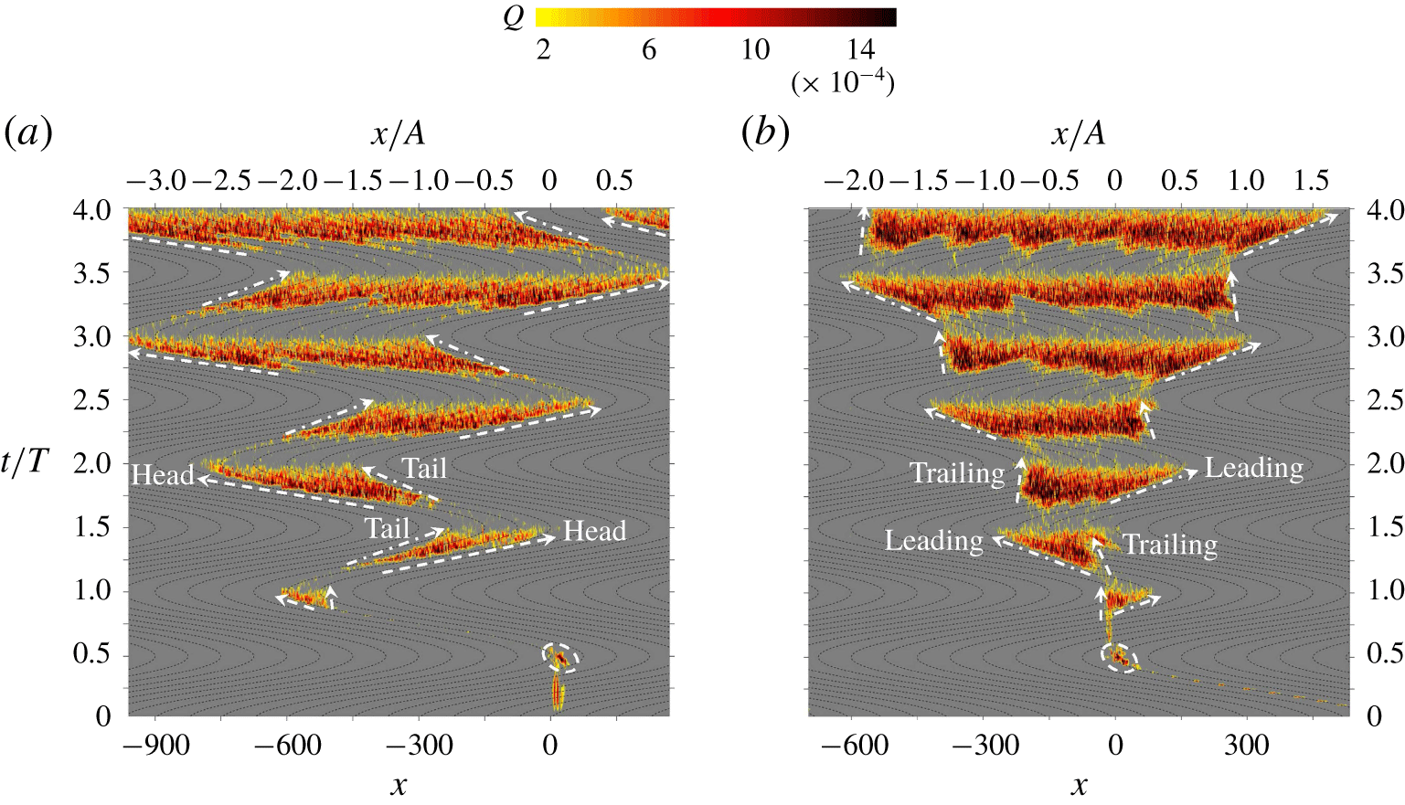
Contour plots of averaged distribution of  $Q^{+}$ along
 $y=1$ of case 16 in the spatio-temporal domain of
 $x$–
 $t/T$ with respect to (a) fixed reference frame
 $S$ and (b) moving reference frame
 ${\hat{S}}$, where the thin dashed lines in the background denote traces of the points attached to the free-stream particle and the oscillating wall, respectively. The first disturbance patches are circled by dashed ellipses. Each sword-shaped strip displayed in the contour plot is bounded by arrows with dashed-dotted lines and dashed lines, which indicate the tail (leading) and head (trailing) edges, respectively, of turbulent spots in the spatio-temporal domain.

4 The propagation of turbulent spots
The spatial propagation characteristics and periodically self-sustaining mechanism of turbulent spots are investigated by taking advantage of a sufficiently long computational domain, and a localised disturbance allows us to track the spatial and temporal evolutions of interrelated coherent structures. Such topics have seldom been covered in previous studies of the Stokes boundary layer. The evolution process is characterised as a looped feedback event of the formation, burst and decay of turbulent spots, as shown in figure 18 and supplementary movie 1 (available at https://doi.org/10.1017/jfm.2020.313). The contour plot shows the  $Q$ distribution in the
 $x$–
 $t/T$ plane, indicating the temporal streamwise variation in the disturbance along the probe line at
 $y=1$ for case 16 at
 $Re=600$ and
 $h=0.5$ in the fixed reference frame
 $S$ and moving reference frame
 ${\hat{S}}$, respectively. The first disturbance patch that was triggered directly by the roughness element (similar to the vortex tube in figure 3) attached to the wall. The disturbance patch experienced transient growth due to the inflection-point instability within the boundary layer until
 $t/T\approx 0.5$. After that, the vortex tube rose into the free stream and disappeared at the slice
 $y=1$. Then, the vortex tube turned back to the boundary layer at
 $t/T\approx 0.8$ (see figure 18a). The first disturbance patch led to the initial turbulent transition of the boundary layer during the deceleration phase. After the inception of the initial turbulence spots (see figure 13), a noteworthy growing zigzag pattern swept across the observation window, following the initial development process of the turbulent spots. The interruption between each sword-shaped strip is the sign of the intermittent emergence and decay of turbulence every half-cycle.
Before starting a further discussion of figure 18, a few definitions to describe the evolution process of streaks and turbulent spots must be clarified to avoid potential confusion caused by the conversion between different reference frames. In the present study, the leading and trailing edges are adopted to describe the sharp and blunt boundaries, respectively, of each sword-shaped strip formed by the streaks, respectively, observed in the moving reference frame (figure 18b). The terms ‘tail’ and ‘head’ were employed in a previous study (Mazzuoli et al. Reference Mazzuoli, Vittori and Blondeaux2011) to describe the back (dash-dotted lines) and front (dashed lines) edges of the contour strips in figure 18(a). The propagation speeds of the tail and head of the spots calculated by the slope of the arrowhead lines are approximately 0.40–0.50 and 0.75–0.85, respectively, in the fixed frame, which are similar to those observed by Mazzuoli et al. (Reference Mazzuoli, Vittori and Blondeaux2011). Correspondingly, the propagation speeds of the leading and trailing edges of the spots are 0.35–0.45 and 0–0.1, respectively, in the moving reference frame. The reason for using different terms in the present study is mainly because a different perspective of the propagation process of the turbulent spots can be achieved by observing the physical process in the moving reference frame.
The main reason for the difference in the propagation speeds of the leading and trailing edges is that the existing free-stream perturbations generally retain their streamwise positions regardless of the oscillatory motion of the boundary wall and continuously trigger the transition of the boundary layer from the middle acceleration phase, while the initial perturbations persist within the viscous sublayer moving together with the boundary wall observed in the reference frame  ${\hat{S}}$. The free-stream perturbations and the initial transient growth of the perturbations in the boundary layer are largely responsible for the formation of the trailing and leading edges of the turbulent spot, respectively, and also give rise to the increasing range of the boundary layer covered by the turbulent spots during the deceleration phase due to an increased level of turbulence in the free stream with the development process of the turbulent spots. As shown in figure 18, each contour strip of the turbulent spots formed during the deceleration phase has a shape similar to a sword in the spatio-temporal domain. Obvious decays of the perturbations are also observed from the late deceleration phase due to the fast dissipation of turbulence from the breakdown of coherent structures and the stabilisation effect by the favourable pressure gradient. Only a small portion of the perturbations remains visible in the middle part of the sword during the acceleration phase, marking the location where the strongest burst of turbulence occurs in the previous stroke (viewing along a vertical line cutting through the strips in figure 18), and the streak structure occurs in the next deceleration phase. We can infer that the bypass mechanism plays a critical role in the regeneration of turbulent spots.
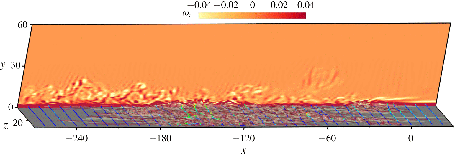
Snapshot showing the streamwise distribution of near-wall flow structures and free-stream vortices at the beginning of the deceleration phase  $t/T=1.750$ of case 16. The streak is indicated by the isosurfaces of transverse vorticity
 $\unicode[STIX]{x1D714}_{y}$ coloured by bright yellow (
 $-0.2$) and red (0.2); the vortex lines are seeded at
 $y=1$ and are coloured by vertical position
 $y$ ranging from 1 (blue) to 3 (red). The background shows the contour of spanwise vorticity
 $\unicode[STIX]{x1D714}_{z}$ at
 $z=0$.

The instantaneous 3-D flow structures of the streak and turbulent spots are visualised in figure 19 to examine the spatial characteristics. The streaks at the trailing (left) and leading (right) edges are still relatively sharp and parallel at this instant, whereas the intensive streaks in the middle are already twisted and irregular. The arch-like vortex lines bridge across each pair of streaks in the trailing and leading areas, and in the middle area, they roll up like a hairpin and incline upwards in the flow direction relative to the wall (from right to left at this instant). The relatively regular shapes of the streaks in the trailing and leading areas can be explained by the relative movement between the fluid mass in the viscous sublayer and the free-stream turbulence generated in the previous stroke, which determines the lifespan of the streaks and the phase duration over which they are subjected to disturbances from the free stream in the Lagrangian view. The streaks in the leading area were generated in the early stage of the deceleration phase and are less affected by the free-stream disturbance due to the short duration of the exposure to the free-stream disturbances. The reason for this short duration is that the wall moves rightwards out of the region covered by the free-stream turbulence generated in the previous oscillation cycle if observed in the moving reference frame  ${\hat{S}}$. The streaks in the trailing area are newly generated and evolve from the laminar boundary layer affected by strong free-stream disturbances. The streaks in the middle area are initialised from the trailing area and are continuously subjected to free-stream disturbances for a longer period of time. The fast transient growth and nonlinear interactions of the high density of streaks lead to the strongest irregularity of the streaks in the middle area.
The temporal evolution of the spanwise energy spectra is examined in figure 20. Except for a peak at  $k_{z}=5$ corresponding to the touchdown of the vortex tube at
 $t/T\approx 0.8$ (see figure 13), the kinetic energy reaches its maximum at the lowest wavenumber during the middle stage of the deceleration phase (
 $\unicode[STIX]{x1D719}\approx 110^{\circ }$ and
 $290^{\circ }$) within each oscillation cycle. In addition, the maximum spanwise energy in each cycle increases monotonically from cycle to cycle with the propagation and intensification of the turbulent spots, as shown in figure 18. No significant change in the waveform is observed in figure 20, indicating that the bypass transition mechanism remains the same in the process. In the middle stage of the acceleration phase (
 $\unicode[STIX]{x1D719}\approx 50^{\circ }$ and
 $230^{\circ }$), the kinetic energy of the 3-D disturbance reaches a minimum. During the acceleration phase, the values of the disturbance energy at higher wavenumbers decay faster than those at lower wavenumbers, suggesting that small-scale turbulent spots dissipate quicker than the large-scale vortex structures.
Temporal evolution of the spectrum of kinetic energy of 3-D disturbance in the spanwise direction of case 16. Thick dotted lines and thin dashed lines indicate the instants when the total kinetic energy of 3-D disturbance reaches maximum and minimum during each half-cycle, respectively.

5 The self-sustaining mechanism
Conceptual model of bypass transition and self-sustainable mechanism for the turbulent spot during a cyclic process that forms a closed feedback loop.

Costamagna et al. (Reference Costamagna, Vittori and Blondeaux2003) and Ozdemir et al. (Reference Ozdemir, Hsu and Balachandar2014) have confirmed that the turbulence in the intermittently turbulent regime is self-sustaining, namely that the periodic emergence of turbulence is independent of external disturbance such as wall imperfections or background perturbation once the coherent structures are fully present. However, the specific self-sustaining mechanism has not been systematically discussed in the literature to the best of the authors’ knowledge. To fill the gap, we propose a conceptual model of the self-sustainable mechanism for the turbulent spot, which is presented in three stages: (I) inception, (II) growth and (III) breakdown of turbulent spots in accordance with figure 21.
(I) Inception: In the middle of the acceleration phase at  $\unicode[STIX]{x1D719}=45^{\circ }$, the optimal perturbations from the free-stream turbulence ejected by the last streak breakdown just trigger the inception of a new streak and hairpin vortex through a receptivity mechanism, which has been described in § 3.2; at the same time, the free-stream turbulence has circulated and would finally dissipate in the outer region of the boundary layer through momentum transfer and diffusion.
(II) Growth: The fastest transient growth of perturbation starts from the late acceleration phase, which is featured by the emergence of intensive streaks and rollup of hairpin vortices under the bypass mechanism as shown in figure 11; the adverse pressure gradient during the deceleration phase continues destabilising the coherent structures.
(III) Breakdown: From the middle deceleration phase, the breakup of hairpin vortex causes the burst of turbulence and ejection into free stream, which is followed by a rapid decay of perturbation energy and an intermittent recovery to a laminar state of boundary layer flow before another stroke starts a repetition from (I).
This physical process summarised in figure 21 is qualitatively suggested by numerical simulations displayed in supplementary movie 1 of the present study and experimental visualisations shown in supplementary movie 2, which is reproduced from supplementary movie 3 of Carstensen et al. (Reference Carstensen, Sumer and Fredsøe2010). The temporal evolution of the total 3-D perturbation energy and vertical distribution of the fluctuations of each velocity component and strength of the vertical structures of saturated flow at  $Re_{\unicode[STIX]{x1D6FF}}=600$ are presented in figures 22 and 23 to facilitate the discussion with quantitative evidence.
(a) The temporal evolution of total 3-D perturbation energy at  $Re_{\unicode[STIX]{x1D6FF}}=600$ and (b) the streamwise spectrum of it from
 $\unicode[STIX]{x1D719}=45^{\circ }$ at
 $t/T=3.125$ to
 $\unicode[STIX]{x1D719}=180^{\circ }$ at
 $t/T=3.500$ with an interval of
 $45^{\circ }$. Markers of each phase instant in (b) are indicated in (a). For reference the inertial scale with the slope of
 $-5/3$ is shown by a solid line.

The vertical distribution of averaged absolute values of fluctuation of three velocity components and  $Q^{+}$ at
 $Re_{\unicode[STIX]{x1D6FF}}=600$; the closed loops indicates the value and position of the temporal peak on the profile.

The temporal evolution of the total 3-D perturbation energy shown in figure 22 indicates that  $E_{3D}$ drops to a trough at
 $\unicode[STIX]{x1D719}=45^{\circ }$. Owing to the stabilisation effect of the favourable pressure gradient, eddies reminiscent of the previous cycle continue dissipating turbulent kinetic energy during the acceleration phase. In addition, the corresponding kinetic energy at
 $\unicode[STIX]{x1D719}=45^{\circ }$ shown in figure 22(b) decreases faster at high wavenumbers than at low wavenumbers, suggesting a quicker dissipation rate for small-scale vortices. The good agreement of the energy spectrum with the well-known scale
 $-5/3$ in the inertial range observed at
 $\unicode[STIX]{x1D719}=45^{\circ }$ demonstrates the isotropic characteristics of the turbulence at this instant.
The vertical profiles of averaged absolute values are examined in figure 23. Each of the profiles of  $|u^{\prime }|$ shown in figure 23(a) is characterised by two peaks: one located in the region near the wall and the other in the outer region. The large
 $|u^{\prime }|$ values surrounding the peak near the wall are generated by the formation and breakdown of streaks, whereas the large
 $|u^{\prime }|$ values surrounding the outer peak are due to perturbations originating from the burst of turbulence into the outer region through momentum transfer and diffusion. By connecting the peaks of
 $|u^{\prime }|$ at different phases in the region near the wall and the outer region, we can obtain two closed loops indicated by the red dotted lines in figure 23(a). The loop in the region near the wall represents the formation and breakdown region of the streaks, while the loop in the outer region provides an indication of the large-scale circulation. The characteristics of
 $|u^{\prime }|$ are not observed in the profiles of
 $|v^{\prime }|$ and
 $|w^{\prime }|$, because the inception of the streaks only has a minor influence on
 $|v^{\prime }|$ and
 $|w^{\prime }|$ in the region near the wall. Similarly, by connecting the peaks of
 $|v^{\prime }|$ and
 $|w^{\prime }|$ at different phases, we can obtain one closed loop for each velocity fluctuation component. The loops indicate the large-scale circulation of the turbulence in the outer region, which can be observed in supplementary movies 1 and 2.
The perturbation energy at low wavenumbers is the strongest at  $\unicode[STIX]{x1D719}=90^{\circ }$ among the four phases examined in figure 22(b), suggesting strong coherent streak structures. The overall growth of
 $E_{3D}$ at this stage is attributed to the relatively lower dissipation rate compared to the production rate of disturbance, as the former only grows rapidly after eddy formation at the inertial scale. Therefore,
 $E_{3D}$ decreases after the instant of the breakup of the coherent structure (figure 22a). The formation of inertial-scale eddies is demonstrated by the dramatic increase of turbulent energy at high wavenumbers at
 $\unicode[STIX]{x1D719}=135^{\circ }$ (figure 22b). Meanwhile, the value of
 $|v^{\prime }|$ shown in figure 23(b) reaches the peak value at
 $y\approx 1.5$, which corresponds to the position of the trough of
 $|u^{\prime }|$ at
 $\unicode[STIX]{x1D719}=135^{\circ }$. This scenario suggests that the centre of the spanwise vortex is located at
 $y\approx 1.5$ and provides evidence for the separation and ejection of the head of the hairpin vortex proposed in the conceptual model (figure 21). The dramatic decrease in
 $|u^{\prime }|$ shown in figure 23(a) occurs immediately after the burst of turbulence (from
 $\unicode[STIX]{x1D719}=135^{\circ }$ to
 $\unicode[STIX]{x1D719}=180^{\circ }$). The
 $y$-locations of the peak values of
 $|v^{\prime }|$ and
 $|w^{\prime }|$ move away from the boundary wall following the breakdown of the streaks
 $\unicode[STIX]{x1D719}\approx 135^{\circ }$ until the subsequent deceleration phase.
The bypass mechanism plays a critical role in triggering turbulent spots and maintaining their self-sustainability in circumstances without external background disturbances or wall imperfections (Costamagna et al. Reference Costamagna, Vittori and Blondeaux2003; Ozdemir et al. Reference Ozdemir, Hsu and Balachandar2014). Furthermore, the free-stream vortex ejected by the last streak breakdown contains the optimal perturbation for the inception of the next streak. For example, when the free-stream flow is from left to right, the head of the hairpin vortex is mainly characterised by negative spanwise vorticity with 3-D disturbance. According to our previous discussion in § 3.2, this characteristic of the head of the hairpin vortex meets the requirement for the optimal free-stream disturbance to trigger the oblique transition in the next deceleration phase. Therefore, the generation and breakdown processes of streaks will repeat in the next half-cycle when the free-stream flow is from right to left, which closes the inception–growth–breakdown feedback loop.
6 Conclusions
A series of 3-D direct numerical simulations are conducted to study the transition of the Stokes boundary layer in the intermittently turbulent regime that is triggered by a roughness element temporarily placed on the wall and a localised vortex disturbance artificially imposed in the flow field. The bypass transition mechanism associated with the onset and evolution of two different coherent structures is the focus of this study. The conclusions are summarised as follows.
The vortex tube triggered by a roughness element of relatively large amplitude is due to an inflection-point instability of the shear layer. A simplified model derived from the Helmholtz point-vortex equation can be used to explain the self-induced circling motion of the vortex pair after it rolls up from the boundary layer. The trajectory of the vortex pair is dependent on the summation and ratio between the strengths of the circulation in each vortex of the pair and the separation distance between the vortices.
The Crow instability leads to a 3-D transition of vortex tubes that are undergoing orbit motion, especially for the weaker one of a counter-rotating vortex pair. The touchdown of the ring-like or quasi-2-D vortex structure evolving from the outer vortex gives rise to streak structures on the boundary if it is in a favourable condition for an oblique transition, followed by the secondary growth of the streak and rollup of hairpin vortices, which are referred to as turbulent spots in the experimental study.
The receptivity mechanism defines a favourable condition that allows a free-stream vortex to trigger an oblique transition. The superposition of the 2-D spanwise vortex with favourable signs of vorticity with a sinusoidal perturbation within a certain distance from the wall can lead to the oblique transition in the boundary layer, which is attributed to the explosive and non-modal transient growth of the perturbations.
The spatial propagation of the turbulent spots is characterised by a noteworthy growing zigzag pattern in the streamwise temporal domain. The velocity difference between the leading and trailing edges (or tail and head) of the turbulent spots is caused by the relative motion between the free-stream disturbance and the wall, which also determines the streamwise distribution of the extent of the turbulence along with the streaks.
The periodically self-sustaining mechanism of the turbulent spots can be summarised as follows. (I) The optimal perturbations from the free-stream turbulence trigger the inception of the streaks through a receptivity mechanism, while most of the free-stream turbulence circulates and finally dissipates in the outer region during the acceleration phase. (II) The fast transient growth of the perturbations due to the bypass mechanism is featured by intensive streaks and the rolling up of hairpin vortices starting from the deceleration phase. (III) The free-stream turbulence ejected by the breakup of hairpin vortices is generally favourable for the reproduction of (I).
Acknowledgements
C.X. would like to acknowledge support from the National Natural Science Foundation of China (no. 51909055), the China Postdoctoral Science Foundation (no. 2019M652480) and the Natural Science Foundation of Hebei Province (no. E2019202471). The authors would like to acknowledge the technical support from the National Supercomputer Center in Tianjin, China, and the Pawsey Supercomputing Centre with funding from the Australian Government and the Government of Western Australia. The authors also acknowledge professors B. M. Sumer and S. Carstensen for providing insightful videos from their experiments.
Declaration of interests
The authors report no conflict of interest.
Supplementary movies
Supplementary movies are available at https://doi.org/10.1017/jfm.2020.313.
Appendix A. Model validation
Comparison of contours of (i) spanwise vorticity  $\unicode[STIX]{x1D714}_{z}$ and (ii) residual of continuity equation with grid lines of
 $h$-type mesh for
 $h=1$ at
 $Re_{\unicode[STIX]{x1D6FF}}=500$. (a) The original contours obtained from the computational domain with a hump at
 $t/T=t_{c}/T\approx 0.531$. (b) The instantaneous ones after mapping onto the computational domain with the smoothed wall at the same instant
 $t=t_{c}$. (c) The updating after only one step of time iteration
 $t=t_{c}+\unicode[STIX]{x0394}t$,
 $\unicode[STIX]{x0394}t/T=5\times 10^{-6}$.

The mesh with an isolated hump is deformed from the mesh with a smoothed wall through solving the linear elasticity equation:
 $$\begin{eqnarray}\unicode[STIX]{x1D735}\boldsymbol{\cdot }[\unicode[STIX]{x1D706}\,\text{Tr}(\unicode[STIX]{x1D640})\unicode[STIX]{x1D644}+\unicode[STIX]{x1D707}\unicode[STIX]{x1D640}]=0,\end{eqnarray}$$
where  $\unicode[STIX]{x1D706}$ and
 $\unicode[STIX]{x1D707}$ are the Lamé constants, and
 $\unicode[STIX]{x1D644}$ represents the identity tensor. The strain tensor
 $\unicode[STIX]{x1D640}$ is defined by
 $$\begin{eqnarray}\unicode[STIX]{x1D640}={\textstyle \frac{1}{2}}(\unicode[STIX]{x1D735}\boldsymbol{S}+(\unicode[STIX]{x1D735}\boldsymbol{S})^{\text{T}}),\end{eqnarray}$$
where  $\boldsymbol{S}$ is the displacement vector with respect to deformation. The only non-trivial boundary condition on the bottom wall is set to
 $\boldsymbol{S}=(0,f(x))$ as prescribed in (2.6). Figure 24(
 $a\text{i}$,
 $b\text{i}$) demonstrates that the mapping of the instantaneous flow field from the computational domain with an isolated roughness element to that with a smoothed wall can be expressed by
 $$\begin{eqnarray}\boldsymbol{u}(\boldsymbol{x}_{i})=\boldsymbol{u}(\boldsymbol{x}_{i}+\boldsymbol{S}_{i}),\end{eqnarray}$$
where  $\boldsymbol{x}_{i}$ and
 $\boldsymbol{S}_{i}$ are the coordinate and displacement vectors on grids of the smoothed-wall mesh. This mapping approach is analogous to mesh update strategies extensively adopted in the computation of flow problems with moving boundaries (Johnson & Tezduyar Reference Johnson and Tezduyar1994). As shown in figure 24(
 $b\text{ii}$) We note that the local continuity may not be strictly guaranteed by the operation of mapping according to the contour of the residual of the continuity equation (
 $\unicode[STIX]{x1D700}_{c}=\unicode[STIX]{x1D735}\boldsymbol{\cdot }\boldsymbol{u}$). However, the amplitude of
 $\unicode[STIX]{x1D700}_{c}$ has already vanished after only one time step
 $\unicode[STIX]{x0394}t/T=5\times 10^{-6}$, as shown in figure 24(
 $c\text{ii}$), while no observable change could be found between the vorticity contours between figures 24(
 $b\text{i}$) and 24(
 $c\text{i}$). This performance is attributed to the IMEX time integration method and the velocity correction scheme adopted in time stepping, which is able to correct the divergence of velocity within just one time step. These results suggest that the influence of the instantaneous residual induced by the mapping operation is negligible for global flow behaviour.
Comparison of the kinetic motion of the primary pair of the positive and negative vortex with three different cutoff times  $t_{c}$ with an interval of
 $\unicode[STIX]{x0394}t/T=1/16$ at
 $Re_{\unicode[STIX]{x1D6FF}}=500$ and
 $h=0.5$ (case 5).

The cutoff time  $t_{c}$ for conducting the mapping operation is carefully selected, as the hump should be removed as soon as possible once the dynamics of the vortex tube is not affected by it. The comparison of the kinetic motion of the vortex pair with three different
 $t_{c}$ with an interval of
 $\unicode[STIX]{x0394}t/T=2/32\approx 0.06$ is presented in figure 25. The result demonstrates that the trajectories of the vortex pair reach convergence after
 $t_{c}/T\approx 0.531$. The animated 3-D flow visualisations are also shown in the supplementary movie 3, which compares the trajectory of the vortex pair and the inception of turbulent spots obtained from the computational domain with a fixed roughness element and the counterpart with a temporary roughness element. Their reasonably good agreement in both results indicates that the key physical mechanism is independent of any artificial effects associated with the mapping operation and cutoff time.
Comparison of trace and amplitude of positive (open) and negative (solid) vortex cores of the primary vortex tubes obtained from the present and refined meshes at  $Re_{\unicode[STIX]{x1D6FF}}=500$ and (a)
 $h=0.25$ (case 4) and (b) 0.5 (case 5), where the circulation of a vortex can be obtained by (3.1) and (3.2).

Comparison of the (a) streamwise energy spectra for different interpolant orders  $N_{p}$ with
 $N_{z}=64$ and (b) spanwise energy spectra for different Fourier modes
 $N_{z}$ with
 $N_{p}=8$, both of which are averaged during
 $3\leqslant t/T\leqslant 4$ at
 $Re_{\unicode[STIX]{x1D6FF}}=600$ and
 $h=0.5$ (case 8). The line for
 $-5/3$ inertial scale is plotted in (a) for reference.

The validation of the 2-D  $h$-type mesh is carried out by comparing the trace and amplitude of the positive and negative vortex cores of the primary vortex tubes obtained from the present mesh (see figure 2 and table 2) and the refined mesh with double resolution over the
 $x{-}y$ plane. The comparison shown in figure 26 suggests that the present 2-D mesh is sufficient to produce converged results when simulating the generation and evolution of the vortex tubes.
The convergence of the  $p$-type refinement is investigated by comparing the streamwise energy spectra of the averaged flows at
 $Re_{\unicode[STIX]{x1D6FF}}=600$ and
 $h=0.5$ with respect to different interpolant orders
 $N_{p}$. As shown in figure 27(a), the kinetic energy for wavenumbers within the range of the large-eddy and inertial scales statistically converges from
 $N_{p}=7$, which demonstrates that the physical phenomena of interest are independent of a further increase in
 $N_{p}$.
The SVV technique employed for the spanwise Fourier modes provides an effective approach to increase the stability and accuracy of the present simulations at a relatively low computational cost. Figure 27 demonstrates that  $N_{z}=64$ is adequate to achieve converged results over the range of wavenumbers that contain the majority (
 ${>}95\,\%$) of the overall 3-D kinetic energy in the saturated state for
 $Re_{\unicode[STIX]{x1D6FF}}=600$. It is noted that the lower Fourier number
 $N_{z}=32$ is adopted for the flows at lower Reynolds numbers
 $Re_{\unicode[STIX]{x1D6FF}}=400$ and 500 because the inception of the coherent structures is our primary interest in these cases, the 3-D instabilities of which are much weaker and only appear for the first few leading spanwise wavenumbers.