1 Introduction
Microorganisms swimming under low Reynolds number conditions use different locomotion strategies. Many studied microswimmers use cilia or flagella (Drescher et al. Reference Drescher, Leptos, Tuval, Ishikawa, Pedley and Goldstein2009; Lauga & Powers Reference Lauga and Powers2009; Guasto, Johnson & Gollub Reference Guasto, Johnson and Gollub2010; Garcia et al. Reference Garcia, berti, Peyla and Rafaï2011; Saintillan & Shelley Reference Saintillan and Shelley2012; Kantsler et al. Reference Kantsler, Dunkel, Polin and Goldstein2013). Prototypical examples are Chlamydomonas reinhardtii, Escherichia coli and Paramecium. Another mode of locomotion, prevalent among eukaryotic cells, albeit much less studied theoretically, is amoeboid motion. This mode is characterized by large deformations of the cell. A prototypical example is Eutreptiella gymnastica (Throndsen Reference Throndsen1969). The name amoeboid is generically used for any motion based on body deformation (be it crawling on a substrate or swimming). Several studies have reported that amoeba such as Dictyostelium (Bae & Bodenschatz Reference Bae and Bodenschatz2010; Barry & Bretscher Reference Barry and Bretscher2010), but also leucocytes (Bae & Bodenschatz Reference Bae and Bodenschatz2010; Aoun et al. Reference Aoun, Negre, Farutin, Garcia-Seyda, Rivzi, Galland, Michelot, Luo, Biarnes-Pelicot and Hivroz2019) or even cancer cells (Pinner & Sahai Reference Pinner and Sahai2008) can swim. Thus, the swimming of these types of microorganisms without adhesion assistance is now gaining more and more interest in the biological literature (Hawkins et al. Reference Hawkins, Piel, Faure-Andre, Lennon-Dumenil, Joanny, Prost and Voituriez2009; Bergert et al. Reference Bergert, Erzberger, Desai, Aspalter, Oates, Charras, Salbreux and Paluch2015; Liu et al. Reference Liu, Le Berre, Lautenschläger, Maiuri, Callan-Jones, Heuzé, Takaki, Voituriez and Piel2015). Understanding amoeboid swimming in a simple fluid has recently incited several theoretical studies (Shapere & Wilczek Reference Shapere and Wilczek1987; Avron, Gat & Kenneth Reference Avron, Gat and Kenneth2004; Ohta & Ohkuma Reference Ohta and Ohkuma2009; Alouges, Desimone & Heltai Reference Alouges, Desimone and Heltai2011; Hiraiwa, Shitara & Ohta Reference Hiraiwa, Shitara and Ohta2011; Vilfan Reference Vilfan2012; Farutin et al. Reference Farutin, Rafaï, Dysthe, Duperray, Peyla and Misbah2013; Loheac, Scheid & Tucsnak Reference Loheac, Scheid and Tucsnak2013; Wu et al. Reference Wu, Thiébaud, Hu, Farutin, Rafaï, Lai, Peyla and Misbah2015, Reference Wu, Farutin, Hu, Thiebaud, Rafai, Peyla, Lai and Misbah2016).
The literature on the wall effect on swimming is quite abundant. The presence of a wall may add several features to the swimming of microorganisms: it may lead to (i) circular trajectories (Smith et al. Reference Smith, Gaffney, Blake and Kirman-Brown2009), (ii) accumulation of swimmers at the wall (Ezhilan & Saintillan Reference Ezhilan and Saintillan2015), (iii) the existence of a stable position of the swimmer at a given distance from the wall (Giacché, Ishikawa & Yamaguchi Reference Giacché, Ishikawa and Yamaguchi2010; Shum, Gaffney & Smith Reference Shum, Gaffney and Smith2010), (iv) rich dynamics of the swimmer orientation and scattering (Crowdy & Or Reference Crowdy and Or2010; Lushi, Kantsler & Goldstein Reference Lushi, Kantsler and Goldstein2017) and so on. A classical way of representing the presence of the walls is via multipolar representation. The first natural step to study swimming in a confined geometry is to represent the swimmer by leading-order terms in far field expansions, which is the Stokeslet dipole. It has been shown (Spagnolie & Lauga Reference Spagnolie and Lauga2012) that the presence of the wall may strongly influence the swimming behaviour.
Our study is focused here on the determination of the swimming speed between two walls, where several numerical observations have not yet been elucidated. Several groups have studied the problem of the influence of confining walls on swimming. Felderhof (Reference Felderhof2010) has reported analytically on a Taylor-like swimmer, showing that the speed is enhanced with confinement. Zhu, Lauga & Brandt (Reference Zhu, Lauga and Brandt2013) have considered numerically the case of a squirmer to show that (when only tangential surface flow is included) the velocity decreases with confinement. When considering normal deformation, they found an increase of velocity with confinement. Liu et al. (Reference Liu, Le Berre, Lautenschläger, Maiuri, Callan-Jones, Heuzé, Takaki, Voituriez and Piel2015) have studied numerically a helical flagellum in a tube and found that, except for a small range of tube radii, the swimming speed, when the helix rotation rate is fixed, increases monotonically as the confinement becomes tighter. Acemoglu & Yesilyurt (Reference Acemoglu and Yesilyurt2014) have adopted a similar model but, besides the flagellum, their swimmer possesses a head and they found a decrease of velocity with confinement. Bilbao et al. (Reference Bilbao, Wajnryb, Vanapalli and Blawzdziewicz2013) have dealt numerically with a model inspired by nematode locomotion and found that it moves faster due to walls. Ledesma-Aguilar & Yeomans (Reference Ledesma-Aguilar and Yeomans2013) have analysed a dipolar swimmer in a rigid or elastic tube and found a speed enhancement due to the walls. Recently, we have studied numerically the case of amoeboid swimmers (Wu et al. Reference Wu, Thiébaud, Hu, Farutin, Rafaï, Lai, Peyla and Misbah2015, Reference Wu, Farutin, Hu, Thiebaud, Rafai, Peyla, Lai and Misbah2016). The velocity was found to decrease slightly with increasing confinement for very wide channels, then to significantly increase for intermediate confinement and finally to decrease to zero as the channel width was further decreased. Understanding of this complex behaviour of amoeboid swimmers is our first focus. It will be shown here that the deformation as well as higher-order effects due to confinement play a decisive role here. We are not aware of any previous study taking these effects into account. We will also consider the case of a squirmer and pumper (undeformable swimmer on the surface of which the normal velocity is prescribed – the swimmer may be thought of as a porous medium pumping fluid) studied numerically (Zhu et al. Reference Zhu, Lauga and Brandt2013).
We build a systematic analytical framework in order to derive the expression of the swimming speed of a microswimmer under confinement. We consider the case of circular swimmers with fixed shape (with tangential or normal flow) and the case of amoeboid swimmers. The obtained analytical expressions agree quantitatively with numerical results for weakly and moderately confined swimmers. For amoeboid swimmers, we observe that the leading effect of confinement (inversely proportional to the square of the channel width) is anomalously small due to an almost-perfect counterbalance of two effects: (i) a wall-induced decrease of the swimming velocity due to a source-dipole term in the multipole expansion of the flow generated by the swimmer and (ii) an increase of the swimming velocity due to swimming in an effective extensional flow which is induced by the walls in reaction to the stresslet of the swimmer. The next-order effect (inversely proportional to the fourth degree of the channel width) has a positive coefficient and is responsible for the increase of the swimming velocity at moderate confinements. For the squirmer case, we find that confinement decreases the speed when tangential flow is considered (the classical case). In the case of normal flow, the speed is enhanced. These results agree with numerical results obtained in three dimensions (Zhu et al. Reference Zhu, Lauga and Brandt2013), despite the fact that our analytical work is developed in two dimensions. This highlights the fact that the dimensionality is irrelevant.
In the case of amoeboid swimmer the treatment is more complex than the squirmer case, due to the free-boundary character. For the sake of analytical tractability, we consider that the swimmer has a shape which is not far from a circle. This allows us to perform a systematic expansion in power series of a small parameter, namely the deviation from a circle. The calculations are simplified by using complex notations for vector variables and representation by analytical functions for multipole expansions.
2 The model
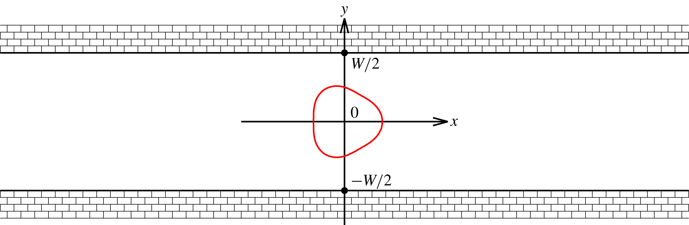
We first consider amoeboid motion as a general case. The case of undeformable swimmers will follow from the general consideration as a particular limit. We use the two-dimensional model introduced in the numerical studies (Wu et al. Reference Wu, Thiébaud, Hu, Farutin, Rafaï, Lai, Peyla and Misbah2015, Reference Wu, Farutin, Hu, Thiebaud, Rafai, Peyla, Lai and Misbah2016) in order to facilitate direct comparison of the results. The system set-up is drawn schematically in figure 1. The swimmer is modelled as an inextensible membrane enclosing a viscous fluid. A time-dependent distribution of active forces normal to the membrane is applied by the swimmer to the inner and outer fluids. The active forces are chosen to be periodic in time, where the period is defined as one stroke cycle. The membrane deforms due to the active forces, which can lead to a net displacement of the swimmer after one stroke, provided the deformation is not time reversible. A translational swimming motion can be achieved by repeating the strokes. We limit this work to the case of swimming along the axis of the channel. It was observed in studies (Wu et al. Reference Wu, Thiébaud, Hu, Farutin, Rafaï, Lai, Peyla and Misbah2015, Reference Wu, Farutin, Hu, Thiebaud, Rafai, Peyla, Lai and Misbah2016) that such centred swimming is not stable and the actual stable mode involves navigation from one wall to the other and back in addition to translation along the channel axis. Nevertheless, the velocity of the translation along the channel axis was found to be close to that in the centred mode.
Amoeboid swimmer in a channel.

The size of the swimmer is characterized by the area of the enclosed fluid
 $A_{0},$
which is conserved due to the impermeability of the membrane and the incompressibility of the fluid inside the swimmer. Another geometric parameter is the perimeter of the swimmer
 $L_{0},$
which we assume to be constant due to the inextensibility of the membrane enclosing the swimmer. These two parameters define a non-dimensional number
 $\unicode[STIX]{x1D70F}\equiv 4\unicode[STIX]{x03C0}A_{0}/L_{0}^{2}$
, which is called the reduced area of the swimmer. A related non-dimensional number is the excess perimeter (counted from the circular shape) defined as
 $$\begin{eqnarray}\unicode[STIX]{x1D6E4}\equiv \frac{L_{0}}{2\unicode[STIX]{x03C0}\sqrt{A_{0}/\unicode[STIX]{x03C0}}}-1=\unicode[STIX]{x1D70F}^{-1/2}-1.\end{eqnarray}$$
We use the excess perimeter
 $\unicode[STIX]{x1D6E4}$
as a small parameter in which the swimming velocity is expanded. The case
 $\unicode[STIX]{x1D6E4}=0$
corresponds to a perfectly circular swimmer, while positive values of
 $\unicode[STIX]{x1D6E4}$
specify the extent of the deformation amplitude.
The swimmer is suspended in a Newtonian fluid of viscosity
 $\unicode[STIX]{x1D702}.$
We assume the interior region of the swimmer to be filled with a fluid having the same viscosity in order to simplify the derivation. Nevertheless, the viscosity of the inner fluid does not affect the swimming velocity in the fully saturated regime which we treat here (i.e. when the active force is so large that the swimmer has enough time to fully develop deformation amplitude available to it before starting a new elementary stroke), as discussed below. The fluids inside and outside the swimmer obey the Stokes equations
 $$\begin{eqnarray}\left.\begin{array}{@{}c@{}}\displaystyle -\unicode[STIX]{x1D735}P(\boldsymbol{r})+\unicode[STIX]{x1D702}\unicode[STIX]{x1D6FB}^{2}\boldsymbol{u}(\boldsymbol{r})=0,\\ \displaystyle \unicode[STIX]{x1D735}\boldsymbol{\cdot }\boldsymbol{u}(\boldsymbol{r})=0,\end{array}\right\}\end{eqnarray}$$
where
 $\boldsymbol{r}$
is the position vector,
 $P$
is the pressure and
 $\boldsymbol{u}$
is the velocity.
The swimmer is confined between two rigid walls separated by a distance
 $W$
(figure 1). We impose the no-slip boundary condition at the walls. The confinement parameter of the problem is defined as
 $C_{n}=2R/W,$
where
 $R=\sqrt{A_{0}/\unicode[STIX]{x03C0}}$
is the characteristic size of the swimmer. We use
 $C_{n}$
as the second small parameter in which the swimming velocity is expanded. The case
 $C_{n}=0$
corresponds formally to an unconfined swimmer. We place the swimmer in the centre of the channel with swimming velocity parallel to the walls. The wall direction is used as the
 $x$
coordinate axis and the swimmer position as the origin (as shown in figure 1).
The motion of the swimmer is actuated by forces applied from the membrane to the fluid. The total force density (force per unit area) at the membrane is composed of an active part and a passive part, and can be written as (Wu et al. Reference Wu, Farutin, Hu, Thiebaud, Rafai, Peyla, Lai and Misbah2016)
 $$\begin{eqnarray}\boldsymbol{f}=\boldsymbol{f}_{a}-\unicode[STIX]{x1D701}c\boldsymbol{n}+\frac{\unicode[STIX]{x2202}\unicode[STIX]{x1D701}}{\unicode[STIX]{x2202}s}\boldsymbol{t}+\boldsymbol{f}_{0}+f_{t}\boldsymbol{t},\end{eqnarray}$$
where
 $\boldsymbol{f}_{a}$
is the density of the active force, which depends on position and time. The exact expression of the density of the active force is chosen below;
 $\unicode[STIX]{x1D701}$
is a Lagrange multiplier that enforces local inextensibility of the membrane,
 $c$
is the curvature,
 $\boldsymbol{t}$
is the unit tangent vector and
 $s$
is the arc length. The constants
 $\boldsymbol{f}_{0}$
and
 $f_{t}$
are added to satisfy the condition of the total force and the total torque exerted by the membrane being equal to zero,
 $$\begin{eqnarray}\oint \boldsymbol{f}\,\text{d}s=0,\quad \oint \boldsymbol{r}\times \boldsymbol{f}\,\text{d}s=0.\end{eqnarray}$$
The symmetry of the problem considered here dictates
 $f_{0y}=f_{t}=0$
.
We use the same expression of the active force as in Wu et al. (Reference Wu, Thiébaud, Hu, Farutin, Rafaï, Lai, Peyla and Misbah2015, Reference Wu, Farutin, Hu, Thiebaud, Rafai, Peyla, Lai and Misbah2016),
 $$\begin{eqnarray}\boldsymbol{f}_{a}(s,t)=2A[\cos (\unicode[STIX]{x1D714}t)\cos (2\unicode[STIX]{x1D6FC})-\sin (\unicode[STIX]{x1D714}t)\cos (3\unicode[STIX]{x1D6FC})]\boldsymbol{n},\end{eqnarray}$$
where
 $t$
is time,
 $\unicode[STIX]{x1D714}$
is the stroke frequency,
 $\unicode[STIX]{x1D6FC}\equiv 2\unicode[STIX]{x03C0}s/L_{0}$
is the rescaled arc length on the swimmer membrane and
 $A$
controls the amplitude of the active stresses. Local incompressibility of the membrane of the swimmer implies that
 $\unicode[STIX]{x1D6FC}$
serves as a reference coordinate of material points on the membrane of the swimmer. Indeed, as the shape of the swimmer evolves with time, the distance along the membrane between any two material points remains constant.
The non-dimensional saturation number
 $S\equiv A/(\unicode[STIX]{x1D702}\unicode[STIX]{x1D714})$
expresses the amplitude of the active stresses compared to the viscous ones. The saturation number
 $S$
can be viewed as a ratio of two time scales: the characteristic time of shape response under the action of active stresses
 $\unicode[STIX]{x1D702}/A$
and the characteristic time over which the active forces change
 $1/\unicode[STIX]{x1D714}.$
Large values of
 $S$
correspond to saturated regime, in which the shape adapt almost instantaneously to the changes of the active stresses. In this study we consider a formal limit of
 $S\rightarrow \infty ,$
which closely resembles the quasi-saturated case of
 $S=10$
used to obtain most of the results in Wu et al. (Reference Wu, Thiébaud, Hu, Farutin, Rafaï, Lai, Peyla and Misbah2015, Reference Wu, Farutin, Hu, Thiebaud, Rafai, Peyla, Lai and Misbah2016). An estimate for
 $S$
was given in Ranganathan, Farutin & Misbah (Reference Ranganathan, Farutin and Misbah2018) for mammalian cells and was found to be of order one. This is a very rough estimate since the cortex viscosity (which is the most relevant one; see Ranganathan et al. (Reference Ranganathan, Farutin and Misbah2018)) is poorly documented. In our previous numerical study (Wu et al.
Reference Wu, Farutin, Hu, Thiebaud, Rafai, Peyla, Lai and Misbah2016) we found that the swimming speed is close to saturation even at
 $S=1$
. In view of this we have opted for the limit where
 $S$
is large enough, a limit which lends itself to a relatively simpler analytical tractability.
The solution to the problem is obtained as a truncated expansion in powers of
 $\unicode[STIX]{x1D6E4}^{1/2}$
(we show below the legitimacy of this choice) and
 $C_{n}.$
The convergence of the expansions for given values of
 $\unicode[STIX]{x1D6E4}$
and
 $C_{n}$
is verified by comparison to full numerical simulations of swimming in confined geometry. The value
 $S=5000$
was used in numerical simulations.
3 Analytical technique
3.1 Complex notation
This section provides the main steps of the analytical solution of the problem. We present explicitly the solution to the leading order in powers of
 $\unicode[STIX]{x1D6E4}$
and
 $C_{n}$
. Higher-order expansions are obtained by following the same procedure but we only provide the final expression for the time-averaged swimming velocity because the intermediate expressions are too long.
It is convenient to view two-dimensional vectors as complex numbers, which we denote by a hat. For example,
 $\hat{r}=r_{x}+\text{i}r_{y}$
. All vector fields on the swimmer membrane can then be represented by periodic complex-valued functions of
 $\unicode[STIX]{x1D6FC}$
. These periodic functions are conveniently represented by Fourier series. For example, the shape of the swimmer is parametrized as
 $$\begin{eqnarray}\hat{r}(\unicode[STIX]{x1D6FC})=\mathop{\sum }_{k=-\infty }^{\infty }r_{k}\text{e}^{\text{i}k\unicode[STIX]{x1D6FC}}.\end{eqnarray}$$
3.2 Quasi-static approximation
The first step is to apply the quasi-static approximation, corresponding to the limit
 $S\rightarrow \infty$
. The stresses in fluids adjacent to the membrane of the swimmer are balanced by the force density acting from the membrane. The velocity and pressure gradients inside the fluids are controlled by the deformation rate of the membrane, which, in turn, is controlled by the stroke frequency in the limit of large
 $S$
. Therefore, the stresses in fluids are small compared to
 $A$
in the limit of large
 $S,$
except for the constant pressure difference
 $\unicode[STIX]{x0394}P$
between the inner and outer fluids. Taking the limit
 $S\rightarrow \infty$
yields for the force balance at the membrane
 $(\boldsymbol{f}+\unicode[STIX]{x0394}P\boldsymbol{n})/A=0$
, where
 $\boldsymbol{n}$
is the normal to the membrane. In other words, the non-hydrostatic stress is irrelevant in the limit of large active forces. This can also be formally seen by appropriate rescaling of variables. Indeed, rescaling time by
 $\unicode[STIX]{x1D714}$
yields in the stress balance a factor
 $\unicode[STIX]{x1D702}\unicode[STIX]{x1D714}$
for the amplitude of the non-hydrostatic stress, to be compared to
 $A$
for the active force. The ratio between the latter and the former provides
 $S$
(which is taken to be large enough in our study). The normal and tangential projections of the simplified force balance equation read, respectively,
 $$\begin{eqnarray}\displaystyle & \displaystyle f_{a}-\unicode[STIX]{x1D701}c+f_{0}n_{x}+\unicode[STIX]{x0394}P=0, & \displaystyle\end{eqnarray}$$
 $$\begin{eqnarray}\displaystyle & \displaystyle \frac{\unicode[STIX]{x2202}\unicode[STIX]{x1D701}}{\unicode[STIX]{x2202}s}+f_{0}t_{x}=0, & \displaystyle\end{eqnarray}$$
where we have omitted the denominator, which is irrelevant for further derivation, in order to simplify the notation. Since
 $t_{x}=\text{d}r_{x}/\text{d}s$
, equation (3.3) can be integrated as
 $$\begin{eqnarray}\unicode[STIX]{x1D701}+f_{0}r_{x}=\unicode[STIX]{x1D701}_{0},\end{eqnarray}$$
where
 $\unicode[STIX]{x1D701}_{0}$
corresponds to the homogeneous part of the tension.
3.3 Small-deformation approximation
We parametrize the shape of the swimmer by the tangent direction as a function of
 $\unicode[STIX]{x1D6FC}$
because this allows us to ensure the local inextensibility of the membrane automatically,
 $$\begin{eqnarray}\frac{\text{d}\hat{r}}{\text{d}\unicode[STIX]{x1D6FC}}=\frac{\text{i}L_{0}}{2\unicode[STIX]{x03C0}}\text{e}^{\text{i}\unicode[STIX]{x1D6FC}}\text{e}^{\text{i}\unicode[STIX]{x1D719}(\unicode[STIX]{x1D6FC})},\end{eqnarray}$$
where
 $\unicode[STIX]{x1D719}(\unicode[STIX]{x1D6FC})$
is a real, time-dependent function used to parametrize the shape of the swimmer. Indeed, the arc element on the swimmer contour is written as
 $\text{d}s=|\text{d}\boldsymbol{r}|=(|\text{d}\boldsymbol{r}|/\text{d}\unicode[STIX]{x1D6FC})\,\text{d}\unicode[STIX]{x1D6FC}$
. Consequently, the absolute value of
 $\text{d}\hat{r}/\text{d}\unicode[STIX]{x1D6FC},$
which is equal to
 $L_{0}/(2\unicode[STIX]{x03C0})$
in (3.5), specifies the local stretching of the swimmer boundary with respect to a circle of radius 1. This shows that parametrization (3.5) allows us to follow not just the shape of the swimmer but also the position of material points on the boundary of a swimmer with a locally inextensible membrane. The argument of
 $\text{d}\hat{r}/\text{d}\unicode[STIX]{x1D6FC}$
, which is equal to
 $\unicode[STIX]{x03C0}/2+\unicode[STIX]{x1D6FC}+\unicode[STIX]{x1D719}(\unicode[STIX]{x1D6FC})$
, specifies the angle which the tangent vector of the swimmer boundary makes with the
 $x$
axis. This is because a unit vector with coordinates
 $(\cos \unicode[STIX]{x1D6FC},\sin \unicode[STIX]{x1D6FC})$
is conveniently written as
 $\text{e}^{\text{i}\unicode[STIX]{x1D6FC}}$
in the complex notation used here. We have split off the
 $\text{e}^{\text{i}\unicode[STIX]{x1D6FC}}$
exponent in (3.5) in order for (3.5) to represent a circle of perimeter
 $L_{0}$
for
 $\unicode[STIX]{x1D719}=0$
. The prefactor
 $i$
could actually be adsorbed in the exponent but we write it here explicitly in order to simplify the final expressions: indeed, imposing the
 $y\rightarrow -y$
symmetry of the problem is equivalent to requiring
 $\unicode[STIX]{x1D719}$
to be an odd function of
 $\unicode[STIX]{x1D6FC}$
. Consequently,
 $\unicode[STIX]{x1D719}$
can be expanded as
 $$\begin{eqnarray}\unicode[STIX]{x1D719}(\unicode[STIX]{x1D6FC})=\mathop{\sum }_{k=-\infty }^{\infty }\unicode[STIX]{x1D719}_{k}\sin (k\unicode[STIX]{x1D6FC}).\end{eqnarray}$$
The small-deformation approximation relies on the amplitudes
 $\unicode[STIX]{x1D719}_{k}$
being small, which allows us to make formal expansions of all shape-related equations. We introduce an expansion parameter
 $\unicode[STIX]{x1D716}$
which expresses the smallness of each particular term. We show below that
 $\unicode[STIX]{x1D716}=O(\unicode[STIX]{x1D6E4}^{1/2})$
. Because the active force (2.5) contains only the second and the third harmonics of
 $\unicode[STIX]{x1D6FC},$
we assume
 $\unicode[STIX]{x1D719}_{2}$
and
 $\unicode[STIX]{x1D719}_{3}$
to be of order
 $O(\unicode[STIX]{x1D716}).$
This ansatz is validated by the consistency of the obtained expansions. The amplitudes
 $\unicode[STIX]{x1D719}_{k}$
for
 $k$
from 4 to 6 are of order
 $O(\unicode[STIX]{x1D716}^{2}),$
and so on. The amplitude
 $\unicode[STIX]{x1D719}_{1}$
is a special case because it can be expressed through the other amplitudes by imposing the consistency condition
 $$\begin{eqnarray}\int _{0}^{2\unicode[STIX]{x03C0}}\frac{\text{d}\hat{r}}{\text{d}\unicode[STIX]{x1D6FC}}\,\text{d}\unicode[STIX]{x1D6FC}=0.\end{eqnarray}$$
Expanding (3.7) in powers of
 $\unicode[STIX]{x1D719}$
yields
 $$\begin{eqnarray}\frac{\text{i}L_{0}}{2\unicode[STIX]{x03C0}}\int _{0}^{2\unicode[STIX]{x03C0}}\text{e}^{\text{i}\unicode[STIX]{x1D6FC}}\left[1+\text{i}\unicode[STIX]{x1D719}(\unicode[STIX]{x1D6FC})-\frac{1}{2}\unicode[STIX]{x1D719}(\unicode[STIX]{x1D6FC})^{2}\right]\text{d}\unicode[STIX]{x1D6FC}+O(\unicode[STIX]{x1D716}^{3})=\frac{\text{i}L_{0}}{2\unicode[STIX]{x03C0}}\left[-\unicode[STIX]{x03C0}\unicode[STIX]{x1D719}_{1}-\frac{\unicode[STIX]{x03C0}\unicode[STIX]{x1D719}_{2}\unicode[STIX]{x1D719}_{3}}{2}\right]+O(\unicode[STIX]{x1D716}^{3})=0.\end{eqnarray}$$
Equation (3.8) shows that
 $\unicode[STIX]{x1D719}_{1}=-\unicode[STIX]{x1D719}_{2}\unicode[STIX]{x1D719}_{3}/2+O(\unicode[STIX]{x1D716}^{3}).$
The amplitudes
 $r_{k}$
in (3.1) are expressed through amplitudes
 $\unicode[STIX]{x1D719}_{k}$
by integrating equation (3.5). The
 $O(\unicode[STIX]{x1D716})$
terms are written as
 $$\begin{eqnarray}\left.\begin{array}{@{}c@{}}\displaystyle r_{-2}=\frac{L_{0}}{8\unicode[STIX]{x03C0}}\unicode[STIX]{x1D719}_{3}+O(\unicode[STIX]{x1D716}^{2}),\quad \displaystyle r_{-1}=\frac{L_{0}}{4\unicode[STIX]{x03C0}}\unicode[STIX]{x1D719}_{2}+O(\unicode[STIX]{x1D716}^{2}),\\ \displaystyle r_{3}=\frac{L_{0}}{12\unicode[STIX]{x03C0}}\unicode[STIX]{x1D719}_{2}+O(\unicode[STIX]{x1D716}^{2}),\quad \displaystyle r_{4}=\frac{L_{0}}{16\unicode[STIX]{x03C0}}\unicode[STIX]{x1D719}_{3}+O(\unicode[STIX]{x1D716}^{2}).\end{array}\right\}\end{eqnarray}$$
The other coefficients
 $r_{k}$
are of higher order. The amplitude
 $r_{1}$
has to be expanded to the next order in order to obtain the leading order of the area inside the swimmer
 $$\begin{eqnarray}r_{1}=\frac{L_{0}}{2\unicode[STIX]{x03C0}}\left(1-\frac{\unicode[STIX]{x1D719}_{2}^{2}+\unicode[STIX]{x1D719}_{3}^{2}}{4}\right)+O(\unicode[STIX]{x1D716}^{3}).\end{eqnarray}$$
The constant part
 $r_{0}$
of expansion (3.1) cannot be deduced from (3.5) because the shape is translationally invariant. For simplicity, we set
 $r_{0}=0$
, effectively choosing the origin to be located in the centre of mass of the membrane of the swimmer. The actual displacement is calculated below by time integration of the velocity of the centre of mass of the membrane. This, together with (3.4), allows us to express the Lagrange multiplier
 $\unicode[STIX]{x1D701}$
through
 $\unicode[STIX]{x1D719}_{k},$
 $\unicode[STIX]{x1D701}_{0}$
and
 $f_{0}$
 $$\begin{eqnarray}\unicode[STIX]{x1D701}=\unicode[STIX]{x1D701}_{0}-\frac{L_{0}f_{0}\cos \unicode[STIX]{x1D6FC}}{2\unicode[STIX]{x03C0}}+O(\unicode[STIX]{x1D716}^{2}),\end{eqnarray}$$
where we assume that
 $f_{0}=O(\unicode[STIX]{x1D716}),$
as is validated below.
The expression for
 $\unicode[STIX]{x1D701}$
is then substituted in (3.2), where the curvature
 $c$
can be conveniently written as
 $$\begin{eqnarray}c=\frac{2\unicode[STIX]{x03C0}}{L_{0}}\left(1+\frac{\text{d}\unicode[STIX]{x1D719}}{\text{d}\unicode[STIX]{x1D6FC}}\right).\end{eqnarray}$$
The consistency of the equations requires us to assume at this point that
 $\unicode[STIX]{x1D701}_{0}$
scales as
 $O(\unicode[STIX]{x1D716}^{-1})$
. Such a non-analytical behaviour of the membrane tension is also encountered for quasi-spherical inextensible membranes in three dimensions (Danker et al.
Reference Danker, Biben, Podgorski, Verdier and Misbah2007). The amplitudes
 $\unicode[STIX]{x1D719}_{k}$
are obtained by solving the
 $k$
th Fourier harmonic (the coefficient of
 $\text{e}^{\text{i}k\unicode[STIX]{x1D6FC}}$
) in (3.2),
 $$\begin{eqnarray}\unicode[STIX]{x1D719}_{2}=\frac{A\cos (\unicode[STIX]{x1D714}t)}{4\unicode[STIX]{x03C0}\unicode[STIX]{x1D701}_{0}}+O(\unicode[STIX]{x1D716}^{2}),\quad \unicode[STIX]{x1D719}_{3}=-\frac{A\sin (\unicode[STIX]{x1D714}t)}{6\unicode[STIX]{x03C0}\unicode[STIX]{x1D701}_{0}}+O(\unicode[STIX]{x1D716}^{2}).\end{eqnarray}$$
The first harmonic of the same equation yields the expansion of
 $f_{0}$
,
 $$\begin{eqnarray}f_{0}=\frac{L_{0}\cos (t)\sin (\unicode[STIX]{x1D714}t)}{48\unicode[STIX]{x03C0}\unicode[STIX]{x1D701}_{0}}.\end{eqnarray}$$
Had we supposed that the tension
 $\unicode[STIX]{x1D701}_{0}$
scales differently, we would then have obtained that the leading shape amplitudes
 $\unicode[STIX]{x1D719}_{2}$
and
 $\unicode[STIX]{x1D719}_{3}$
vanish, which is absurd (no symmetry constraint imposes vanishing of
 $\unicode[STIX]{x1D719}_{2}$
and
 $\unicode[STIX]{x1D719}_{3}$
). The zeroth harmonic can be used to calculate the pressure difference
 $\unicode[STIX]{x0394}P$
but this quantity is not needed for the subsequent calculations. At this point the only quantity remaining unknown is the value of
 $\unicode[STIX]{x1D701}_{0}$
. The expression of
 $\unicode[STIX]{x1D701}_{0}$
is obtained by calculating the area inside the swimmer as
 $$\begin{eqnarray}\displaystyle A_{0} & = & \displaystyle \frac{1}{2}\text{Im}\int _{0}^{2\unicode[STIX]{x03C0}}\hat{r}\frac{\text{d}\hat{r}^{\ast }}{\text{d}\unicode[STIX]{x1D6FC}}\,\text{d}\unicode[STIX]{x1D6FC}=\frac{L_{0}^{2}}{4\unicode[STIX]{x03C0}}\left[1-\frac{9}{16}\unicode[STIX]{x1D719}_{2}^{2}-\frac{2}{3}\unicode[STIX]{x1D719}_{3}^{2}+O(\unicode[STIX]{x1D716}^{3})\right]\nonumber\\ \displaystyle & = & \displaystyle \frac{L_{0}^{2}}{4\unicode[STIX]{x03C0}}\left[1-\frac{L_{0}^{2}}{64\unicode[STIX]{x03C0}^{2}\unicode[STIX]{x1D701}_{0}^{2}}\sin ^{2}(\unicode[STIX]{x1D714}t)-\frac{L_{0}^{2}}{24\unicode[STIX]{x03C0}^{2}\unicode[STIX]{x1D701}_{0}^{2}}\cos ^{2}(\unicode[STIX]{x1D714}t)+O(\unicode[STIX]{x1D716}^{3})\right].\end{eqnarray}$$
Substituting equation (3.15) into (2.1) yields the expansion of
 $\unicode[STIX]{x1D701}_{0}$
in powers of
 $\unicode[STIX]{x1D6E4}$
with time-dependent coefficients.
 $$\begin{eqnarray}\unicode[STIX]{x1D6E4}=\frac{1}{3}\unicode[STIX]{x1D719}_{2}^{2}+\frac{9}{32}\unicode[STIX]{x1D719}_{3}^{2}+O(\unicode[STIX]{x1D716}^{3})=\frac{L_{0}^{2}[5\cos ^{2}(\unicode[STIX]{x1D714}t)+3]}{384\unicode[STIX]{x03C0}^{2}\unicode[STIX]{x1D701}_{0}^{2}}+O(\unicode[STIX]{x1D716}^{3}).\end{eqnarray}$$
This equation clearly shows that the deviation from the circular shape, measured by
 $\unicode[STIX]{x1D719}_{k}$
, is indeed of order
 $\unicode[STIX]{x1D6E4}^{1/2}$
, as anticipated. Equation (3.16) has two solutions for
 $\unicode[STIX]{x1D701}_{0}$
as a function of
 $\unicode[STIX]{x1D6E4}$
, only one of which is stable against shape perturbation for finite
 $S$
. This can be seen by referring to the shape evolution equation (4) (Farutin et al.
Reference Farutin, Rafaï, Dysthe, Duperray, Peyla and Misbah2013) (valid for small
 $\unicode[STIX]{x1D6E4}$
) where linear stability analysis shows that the steady-state solution is unstable for
 $\unicode[STIX]{x1D701}_{0}<0$
. A physical argument is that
 $\unicode[STIX]{x1D701}_{0}<0$
corresponds to the situation where the membrane is under compression, which leads to buckling.
The solution reads
 $$\begin{eqnarray}\unicode[STIX]{x1D701}_{0}=\frac{L_{0}[18+30\cos ^{2}(\unicode[STIX]{x1D714}t)]^{1/2}}{48\unicode[STIX]{x03C0}\unicode[STIX]{x1D6E4}^{1/2}}.\end{eqnarray}$$
3.4 Unconfined swimming
Once the shape of the swimmer is reconstructed as a function of time, the swimming velocity can be obtained by solving the Stokes equation outside of the swimmer. The velocity at the membrane is obtained as
 $$\begin{eqnarray}\boldsymbol{u}(\unicode[STIX]{x1D6FC},t)=v_{s}+\frac{\text{d}\boldsymbol{r}(\unicode[STIX]{x1D6FC},t)}{\text{d}t},\end{eqnarray}$$
where
 $v_{s}$
is the swimming velocity to be solved for. The deformation rate can be expressed using the complex notation as
 $$\begin{eqnarray}\frac{\text{d}\hat{r}(\unicode[STIX]{x1D6FC},t)}{\text{d}t}=\mathop{\sum }_{k\neq 0}\frac{\text{d}r_{k}}{\text{d}t}\text{e}^{\text{i}k\unicode[STIX]{x1D6FC}}.\end{eqnarray}$$
The solution of the Stokes equation (2.2) can be expanded in multipoles as follows. The complex coordinate is denoted as
 $z=x+\text{i}y$
and its conjugate as
 $z^{\ast }$
. A general solution of (2.2) can be written (as recalled in appendix A) as
 $$\begin{eqnarray}\hat{u} =A(z)-z[A^{\prime }(z)]^{\ast }+[B(z)]^{\ast },\end{eqnarray}$$
where
 $A(z)$
and
 $B(z)$
are complex functions that are analytic in the fluid domain. The functions
 $A(z)$
and
 $B(z)$
can be expanded in a series at infinity for the case of unconfined swimmer
 $$\begin{eqnarray}A(z)=\mathop{\sum }_{k=1}^{\infty }\frac{a_{k}}{z^{k}},\quad B(z)=\mathop{\sum }_{k=1}^{\infty }\frac{b_{k}}{z^{k}},\end{eqnarray}$$
where
 $b_{1}=0$
because the volume of the swimmer is conserved (
 $\text{Re}\,b_{1}=0$
) and the total torque acting on the swimmer is zero (
 $\text{Im}\,b_{1}=0$
). The expansion (3.21) incorporates the condition of the swimmer being force free because terms proportional to
 $\ln (z)$
would have to be added to functions
 $A$
and
 $B$
otherwise. The symmetry of the problem dictates that
 $a_{k}$
and
 $b_{k}$
be real. The coefficients
 $a_{k}$
and
 $b_{k}$
are expanded in powers of
 $\unicode[STIX]{x1D6E4}$
as
 $$\begin{eqnarray}a_{k}=\mathop{\sum }_{l=1}^{\infty }a_{k,l}\unicode[STIX]{x1D6E4}^{l/2},\quad b_{k}=\mathop{\sum }_{l=1}^{\infty }b_{k,l}\unicode[STIX]{x1D6E4}^{l/2}.\end{eqnarray}$$
The next step is to substitute the expansions (3.21) and (3.22) into (3.20) and match the resulting flow field to the membrane velocity for
 $z=\hat{r}(\unicode[STIX]{x1D6FC})$
.
Now we use the expression of the velocity field (3.20) evaluated at the swimmer surface and impose (3.18) (continuity of the velocity field). The shape coefficients
 $r_{k}$
in (3.1) have been already determined (see (3.9)–(3.10)) as functions of
 $\unicode[STIX]{x1D719}_{k}$
(defined in (3.6)). Expansion of (3.20) at the swimmer surface in powers of the small amplitude
 $\unicode[STIX]{x1D719}_{k}$
will generate various harmonics
 $\text{e}^{\text{i}m\unicode[STIX]{x1D6FC}}$
(with
 $m$
an integer). Using (3.18) and equating Fourier coefficients provides us relations between different coefficients. The zeroth Fourier harmonic relation yields the swimming velocity
 $v_{s}$
. Note that the leading term of the swimming velocity requires expanding (3.20) to the order of
 $\unicode[STIX]{x1D6E4}$
, and we obtain
 $$\begin{eqnarray}v_{s}=-\frac{\unicode[STIX]{x03C0}^{2}\cos (\unicode[STIX]{x1D714}t)\unicode[STIX]{x1D6E4}^{1/2}}{L_{0}^{2}[18+30\cos ^{2}(\unicode[STIX]{x1D714}t)]^{1/2}}(a_{2}+b_{2})+\frac{3\unicode[STIX]{x03C0}^{3}\sin (\unicode[STIX]{x1D714}t)\unicode[STIX]{x1D6E4}^{1/2}}{8L_{0}^{3}[18+30\cos ^{2}(\unicode[STIX]{x1D714}t)]^{1/2}}(a_{3}+b_{3})+O(\unicode[STIX]{x1D6E4}^{3/2}).\end{eqnarray}$$
Exploiting the relations following from the
 $k$
th and
 $-k$
th Fourier harmonics of (3.20) allows us to determine
 $a_{k}$
and
 $b_{k}$
at the desired order. The leading-order calculation yields
 $$\begin{eqnarray}\displaystyle & \displaystyle a_{2}=\frac{12L_{0}^{3}\unicode[STIX]{x1D714}\cos (\unicode[STIX]{x1D714}t)\unicode[STIX]{x1D6E4}^{1/2}}{\unicode[STIX]{x03C0}^{3}[18+30\cos ^{2}(\unicode[STIX]{x1D714}t)]^{3/2}}+O(\unicode[STIX]{x1D6E4}^{3/2}), & \displaystyle\end{eqnarray}$$
 $$\begin{eqnarray}\displaystyle & \displaystyle b_{2}=-\frac{L_{0}^{3}\unicode[STIX]{x1D714}[9-73\cos ^{2}(\unicode[STIX]{x1D714}t)]\unicode[STIX]{x1D6E4}}{8\unicode[STIX]{x03C0}^{3}[3+5\cos ^{2}(\unicode[STIX]{x1D714}t)]^{2}}+O(\unicode[STIX]{x1D6E4}^{3/2}), & \displaystyle\end{eqnarray}$$
 $$\begin{eqnarray}\displaystyle & \displaystyle b_{3}=-\frac{9L_{0}^{4}\unicode[STIX]{x1D714}\sin (\unicode[STIX]{x1D714}t)\unicode[STIX]{x1D6E4}^{1/2}}{\unicode[STIX]{x03C0}^{4}[18+30\cos ^{2}(\unicode[STIX]{x1D714}t)]^{3/2}}+O(\unicode[STIX]{x1D6E4}),\quad a_{3}=O(\unicode[STIX]{x1D6E4}). & \displaystyle\end{eqnarray}$$
Substituting (3.24)–(3.26) into (3.23) yields
 $$\begin{eqnarray}v_{s}=\frac{L_{0}\unicode[STIX]{x1D714}\unicode[STIX]{x1D6E4}[7\cos ^{2}(\unicode[STIX]{x1D714}t)+9]}{[18+30\cos ^{2}(\unicode[STIX]{x1D714}t)]^{2}}+O(\unicode[STIX]{x1D6E4}^{3/2}).\end{eqnarray}$$
3.5 Confinement effects
Equation (3.20) remains valid in the confined case but the domain where functions
 $A(z)$
and
 $B(z)$
can be considered analytic is now contained inside the strip interior to the walls. Therefore, their Laurent series about the origin contains all integer powers of
 $z$
,
 $$\begin{eqnarray}A(z)=\mathop{\sum }_{k=1}^{\infty }\frac{a_{k}}{z^{k}}+\mathop{\sum }_{k=0}^{\infty }c_{k}z^{k},\quad B(z)=\mathop{\sum }_{k=1}^{\infty }\frac{b_{k}}{z^{k}}+\mathop{\sum }_{k=0}^{\infty }d_{k}z^{k}.\end{eqnarray}$$
The coefficient
 $c_{0}$
is assumed to be equal to zero below, which we can do without loss of generality: indeed, both
 $c_{0}$
and
 $d_{0}$
define a constant contribution to the velocity field when (3.28) is substituted into (3.20). The coefficients
 $c_{k}$
and
 $d_{k}$
can be expressed as a linear combination of
 $a_{k^{\prime }}$
,
 $a_{k^{\prime }}^{\ast }$
,
 $b_{k^{\prime }}$
and
 $b_{k^{\prime }}^{\ast }$
by imposing zero flow at the walls. These linear combinations come in form of infinite sums, the explicit analytical expression of which seems to be unavailable. We therefore resorted to approximate numerical calculations for this part. We simplify the following expressions by using the
 $y\rightarrow -y$
symmetry of the problem, which dictates the coefficients in expansion (3.28) to be real. In this case, the coefficient
 $c_{1}$
can be taken equal to zero: indeed, substituting expansions (3.28) into (3.20) shows that only the imaginary part of
 $c_{1}$
enters the velocity field. The practical method can be described by the following algorithm:
(i) For each value of
 $k$
, we calculate the residual velocity at the walls for a point singularity
$A(z)=1/z^{k}$
,
$B(z)=0$
or
$A(z)=0$
,
$B(z)=1/z^{k}.$
(ii) We then find the wall forces which would cancel the wall velocity computed in the previous step.
(iii) The final step is to calculate at the origin the velocity and its derivatives due to the wall forces found in the previous step.


The second and third steps have to be performed numerically, which can be done with high precision using Fourier representation of the residual velocity and forces at the wall. The derivatives of the velocity field define the coefficients
 $c_{k}$
and
 $d_{k}$
in (3.28). We can thus write using the linearity of (3.28)
 $$\begin{eqnarray}c_{k}=\mathop{\sum }_{k^{\prime }=1}^{\infty }\frac{c_{k}^{ak^{\prime }}a_{k^{\prime }}+c_{k}^{bk^{\prime }}b_{k^{\prime }}}{W^{k+k^{\prime }}},\quad d_{k}=\mathop{\sum }_{k^{\prime }=1}^{\infty }\frac{\text{d}_{k}^{ak^{\prime }}a_{k^{\prime }}+d_{k}^{bk^{\prime }}b_{k^{\prime }}}{W^{k+k^{\prime }}},\end{eqnarray}$$
where the coefficients
 $c_{k}^{ak^{\prime }}$
and so on are dimensionless numbers obtained numerically as described above. These numbers do not depend on
 $W$
because the width of the channel is the only length scale relevant in expansion (3.29). Expansion (3.29) corresponds to the no-slip condition on the channel walls. The form of the solution (3.29) can be understood simply. Indeed, when applying the no-slip boundary condition at the wall on (3.28), one obtains an infinite set of linear equations for the coefficients
 $a_{k}$
,
 $b_{k}$
,
 $c_{k}$
and
 $d_{k}$
, so that
 $c_{k}$
and
 $d_{k}$
are obviously linearly related to
 $a_{k}$
,
 $b_{k}$
. The dependence on
 $W$
can be understood by rescaling
 $z$
by
 $W$
in (3.28), giving rise to
 $W^{-k}$
and
 $W^{k}$
in the first and second sums respectively.
The system is closed by imposing the velocity field (3.20) to be equal to the membrane velocity (3.18) at the boundary of the swimmer, as was done for the unconfined case. This allows us to compute the swimming velocity as a function of confinement.
As a practical demonstration of the method, we present here the intermediate steps for the derivation of the leading-order effect of the confinement. Retaining the terms up to
 $O(C_{n}^{2})$
, we can write
 $$\begin{eqnarray}d_{0}=\frac{d_{0}^{a2}a_{2}+d_{0}^{b2}b_{2}}{W^{2}},\quad d_{1}=\frac{d_{1}^{a1}a_{1}}{W^{2}}.\end{eqnarray}$$
Here, we use that
 $c_{1}=0$
,
 $c_{0}=0$
and
 $b_{1}=0$
, as discussed above. We also use that the coefficient
 $d_{0}^{a1}$
(defining the contribution of
 $a_{1}$
to
 $d_{0}$
) is equal to 0, as follows from the
 $x\rightarrow -x$
symmetry of the problem. Numerical calculation shows that
 $d_{0}^{a2}=3.7719$
,
 $d_{0}^{b2}=-6.8975$
and
 $d_{1}^{a1}=-10.6695$
. Interestingly, we observe that
 $$\begin{eqnarray}d_{1}^{a1}=d_{0}^{b2}-d_{0}^{a2}.\end{eqnarray}$$
This is not a numerical coincidence but a consequence of the invariance of the problem under translation along the
 $x$
axis. Indeed, substituting
 $z\rightarrow z+\text{d}x$
, where
 $\text{d}x$
is real, in (3.20) yields a velocity field that still satisfies the no-slip boundary conditions at the walls. Taking the derivative with respect to
 $\text{d}x$
and setting
 $\text{d}x=0,$
yields that, if velocity field (3.20) satisfies no-slip boundary conditions at the channel walls for certain functions
 $A(z)$
and
 $B(z)$
, then it would also satisfy them if we replace
 $A(z)$
with
 $A^{\prime }(z)$
and
 $B(z)$
with
 $B^{\prime }(z)-A^{\prime }(z)$
. This implies that expansions (3.29) remain valid if we replace
 $a_{k+1}$
with
 $-ka_{k}$
,
 $c_{k-1}$
with
 $kc_{k}$
,
 $b_{k+1}$
with
 $k(a_{k}-b_{k})$
and
 $d_{k-1}$
with
 $k(d_{k}-c_{k})$
. Applying this transformation to the first equation of (3.30) and comparing the result with the second one yields the relation (3.31).
The expression of the swimming velocity in the confined case reads
 $$\begin{eqnarray}\displaystyle v_{s} & = & \displaystyle -\frac{\unicode[STIX]{x03C0}^{2}\cos (\unicode[STIX]{x1D714}t)\unicode[STIX]{x1D6E4}^{1/2}}{L_{0}^{2}[18+30\cos ^{2}(\unicode[STIX]{x1D714}t)]^{1/2}}(a_{2}+b_{2})+\frac{3\unicode[STIX]{x03C0}^{3}\sin (\unicode[STIX]{x1D714}t)\unicode[STIX]{x1D6E4}^{1/2}}{8L_{0}^{3}[18+30\cos ^{2}(\unicode[STIX]{x1D714}t)]^{1/2}}(a_{3}+b_{3})\nonumber\\ \displaystyle & & \displaystyle +\,\frac{d_{0}^{a2}a_{2}+d_{0}^{b2}b_{2}}{W^{2}}+O(C_{n}^{3})+O(\unicode[STIX]{x1D6E4}^{3/2}).\end{eqnarray}$$
The coefficients
 $a_{k}$
and
 $b_{k}$
differ from the ones listed in (3.24)–(3.26) only in higher-order terms (i.e. to the desired order those expressions remain still valid here), except for
 $a_{1}$
and
 $b_{3}$
, which read
 $$\begin{eqnarray}\displaystyle & \displaystyle a_{1}=-\frac{27\unicode[STIX]{x1D714}\sin (\unicode[STIX]{x1D714}t)L_{0}^{2}\unicode[STIX]{x1D6E4}^{1/2}}{\unicode[STIX]{x03C0}^{2}[18+30\cos ^{2}(\unicode[STIX]{x1D714}t)]}\left[1-d_{1}^{a1}\frac{L_{0}^{2}}{4\unicode[STIX]{x03C0}^{2}W^{2}}+O(C_{n}^{3})\right]+O(\unicode[STIX]{x1D6E4}), & \displaystyle\end{eqnarray}$$
 $$\begin{eqnarray}\displaystyle & \displaystyle b_{3}=-\frac{9L_{0}^{4}\unicode[STIX]{x1D714}\sin (\unicode[STIX]{x1D714}t)\unicode[STIX]{x1D6E4}^{1/2}}{\unicode[STIX]{x03C0}^{4}[18+30\cos ^{2}(\unicode[STIX]{x1D714}t)]^{3/2}}-\frac{27d_{1}^{a1}L_{0}^{6}\unicode[STIX]{x1D714}\sin (\unicode[STIX]{x1D714}t)\unicode[STIX]{x1D6E4}^{1/2}}{16\unicode[STIX]{x03C0}^{6}[18+30\cos ^{2}(\unicode[STIX]{x1D714}t)]^{3/2}W^{2}}+O(\unicode[STIX]{x1D6E4}).\qquad & \displaystyle\end{eqnarray}$$
Substituting the expressions for
 $a_{k}$
and
 $b_{k}$
into (3.32) yields the final expression
 $$\begin{eqnarray}v_{s}=\frac{L_{0}\unicode[STIX]{x1D714}\unicode[STIX]{x1D6E4}[7\cos ^{2}(\unicode[STIX]{x1D714}t)+9]}{[18+30\cos ^{2}(\unicode[STIX]{x1D714}t)]^{2}}+\frac{L_{0}^{3}\unicode[STIX]{x1D714}\unicode[STIX]{x1D6E4}[(73\cos ^{2}(\unicode[STIX]{x1D714}t)-9)d_{0}^{b2}-9\sin ^{2}(\unicode[STIX]{x1D714}t)d_{1}^{a1}]}{8\unicode[STIX]{x03C0}^{3}W^{2}[3+5\cos ^{2}(\unicode[STIX]{x1D714}t)]^{2}}+O(\unicode[STIX]{x1D6E4}^{3/2}).\end{eqnarray}$$
4 Results
4.1 Instantaneous velocity
In the previous section we have given the contribution to the swimming velocity to the leading order in confinement, which turns out to be of order
 $C_{n}^{2}$
(or inversely proportional to
 $W^{2}$
). However, the procedure outlined above can be applied in order to expand the swimming velocity to any order in confinement and excess perimeter. In order to dispose of a wider range of applicability of the expansion, we have systematically performed it by retaining terms up to order
 $O(\unicode[STIX]{x1D6E4}^{3})$
and
 $O(C_{n}^{18})$
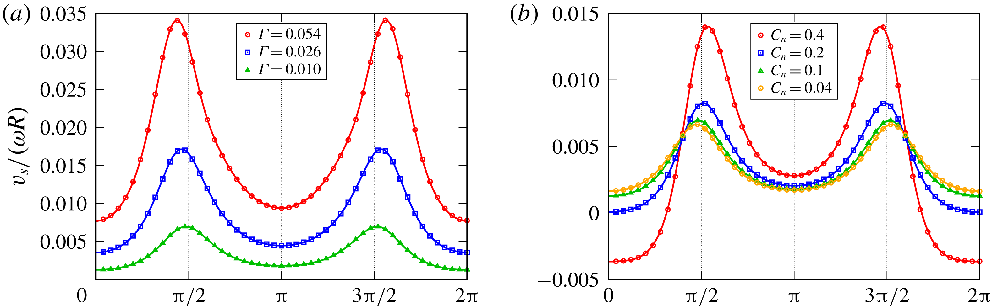
. We have also validated the correctness and the convergence of the analytical results by full numerical simulations. The comparison of swimming velocity obtained analytically and by numerical simulations is shown in figure 2 as a function of time. As can be seen, the agreement is quite satisfactory. Nevertheless, increasing
 $C_{n}$
and
 $\unicode[STIX]{x1D6E4}$
beyond the shown values leads to a noticeable deviation of the analytical results from full numerical simulations (not shown in figure 2).
The velocity of a swimmer
 $v_{s}$
as a function of time. The results of the analytical expansions (shown by continuous curves) are compared with the numerical results (shown by symbols). (a) Fixed confinement
 $C_{n}=0.1$
. (b) Fixed excess perimeter
 $\unicode[STIX]{x1D6E4}=0.010$
.

4.2 Average velocity
The instantaneous swimming velocity can be integrated in time to obtain the displacement over one stroke cycle
 $\unicode[STIX]{x0394}X$
. The resulting series is sufficiently simple to be analysed in detail. In the absence of walls, the displacement
 $\unicode[STIX]{x0394}X$
reads
 $$\begin{eqnarray}\unicode[STIX]{x0394}X=R\unicode[STIX]{x1D6E4}[2.1376-2.1621\unicode[STIX]{x1D6E4}+1.4287\unicode[STIX]{x1D6E4}^{2}+O(\unicode[STIX]{x1D6E4}^{3})]\end{eqnarray}$$
as a function of the excess perimeter.
The dependence of
 $\unicode[STIX]{x0394}X$
on confinement can be analysed by truncating the expansion in powers of
 $\unicode[STIX]{x1D6E4}$
at the leading order. The swimming speed is obtained as
 $\unicode[STIX]{x0394}X/T$
, where
 $T=2\unicode[STIX]{x03C0}/\unicode[STIX]{x1D714}$
is the cycle period,
 $$\begin{eqnarray}\displaystyle v_{s} & = & \displaystyle \frac{R\unicode[STIX]{x1D6E4}}{T}\left[2.1376-0.39748C_{n}^{2}+18.933C_{n}^{4}-52.316C_{n}^{6}+151.86C_{n}^{8}-448.34C_{n}^{10}\right.\nonumber\\ \displaystyle & & \displaystyle +\left.1374.5C_{n}^{12}-4230.7C_{n}^{14}+12851.C_{n}^{16}-38256.C_{n}^{18}+O(C_{n}^{20})\right]+O(\unicode[STIX]{x1D6E4}^{2}).\qquad\end{eqnarray}$$
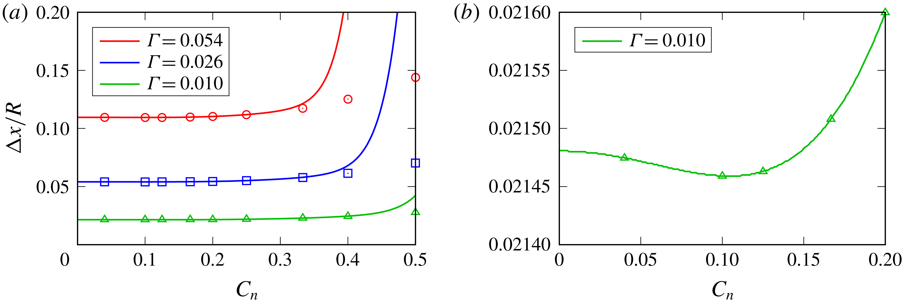
Figure 3 shows the displacement
 $\unicode[STIX]{x0394}X$
as a function of confinement for several values of the excess perimeter.
Displacement of the swimmer after one stroke cycle as a function of the confinement for several values of the reduced volume. Comparison of analytical expansions (solid curves) with numerical simulations (symbols). (b) Shows the magnified view of the case
 $\unicode[STIX]{x1D6E4}=0.010$
highlighting the initial decrease of the swimming velocity with increasing confinement.

Comparison of numerical and analytical results in figure 3 shows that the expansion (4.2) converges provided
 $C_{n}$
is small enough. The ratio of the subsequent coefficients in (4.2) is close to
 $-3$
. This suggests that the region of convergence of this expansion is about
 $C_{n}^{2}<1/3$
. Higher-order terms in
 $\unicode[STIX]{x1D6E4}$
in the expansion (4.2), however, have a smaller radius of convergence. This explains why the analytical curves in figure 3 start to deviate from the numerical results at lower values of
 $C_{n}$
as
 $\unicode[STIX]{x1D6E4}$
is increased.
5 Swimming with fixed shape
5.1 Propulsion by tangential flow
There are several swimmers for which the activity can be modelled by tangential flow. A prototypical example is the paramecium (Zhang et al. Reference Zhang, Jana, Giarra, Vlachos and Jung2015). The corresponding model is known as a squirmer, introduced by Lighthill (Reference Lighthill1952) and reconsidered later by Blake (Reference Blake1971), and has now become a very popular model (Lauga & Powers Reference Lauga and Powers2009). In a completely different field, that of mammalian cells, it was recently suggested (Aoun et al. Reference Aoun, Negre, Farutin, Garcia-Seyda, Rivzi, Galland, Michelot, Luo, Biarnes-Pelicot and Hivroz2019) that the swimming of immune cells (T-lymphocyte) is actuated by the retrograde flow of actin, which is transmitted to the outside fluid by transmembrane proteins, such as integrins. It is therefore an interesting question to see how confinement would affect this mode of locomotion.
The simplest model of a swimmer that uses tangential flow for locomotion in a shape-preserving manner is that of a squirmer. Here we consider a circular squirmer located in the centre of a channel. The flow at the boundary of the swimmer is written as
 $$\begin{eqnarray}\boldsymbol{u}(\unicode[STIX]{x1D6FC})=\boldsymbol{v}_{s}+v_{t}(\unicode[STIX]{x1D6FC})\boldsymbol{t}(\unicode[STIX]{x1D6FC})\equiv \boldsymbol{v}_{s}+(\boldsymbol{v}_{t}^{0}\boldsymbol{\cdot }\boldsymbol{t})\boldsymbol{t},\end{eqnarray}$$
in the laboratory frame. Here
 $v_{t}(\unicode[STIX]{x1D6FC})$
is the local amplitude of the tangential velocity in the swimmer frame. We take
 $v_{t}=v_{t}^{0}\sin \unicode[STIX]{x1D6FC}\equiv \boldsymbol{v}_{t}^{0}\boldsymbol{\cdot }\boldsymbol{t}$
(with
 $\boldsymbol{v}_{t}^{0}$
pointing along the swimming
 $x$
-direction), which is often considered as a model for ciliated organisms. The solution process is similar to the one used for amoeboid swimmers but is simpler because the shape of the swimmer is precisely circular and the flow field is prescribed and constant in time. We thus need to replace (3.18), used for amoeboid swimmers, with (5.1) and recalculate
 $v_{s}$
using the same procedure as before. The calculations yield
 $$\begin{eqnarray}\displaystyle & & \displaystyle \hspace{-36.0pt}v_{sx}=-v_{t}^{0}\left[{\textstyle \frac{1}{2}}-0.86219C_{n}^{2}+0.76452C_{n}^{4}-0.97679C_{n}^{6}+1.7022C_{n}^{8}-3.7459C_{n}^{10}\right.\nonumber\\ \displaystyle & & \displaystyle \hspace{-36.0pt}\quad \left.+\,9.2095C_{n}^{12}-23.687C_{n}^{14}+62.038C_{n}^{16}-163.97C_{n}^{18}+435.74C_{n}^{20}+O(C_{n}^{22})\right].\end{eqnarray}$$
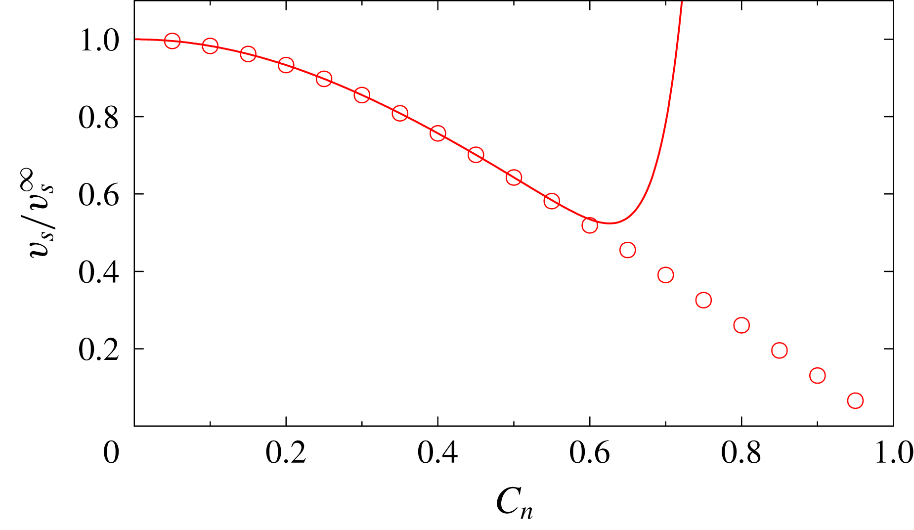
The results obtained by (5.2) and by direct numerical simulations are shown in figure 4. Here again, we see a good agreement between the numerical and analytical results up to a confinement of approximately
 $C_{n}=0.6$
.
Swimming velocity of a squirmer
 $v_{s}=|v_{sx}|$
as a function of confinement, non-dimensionalized by the swimming velocity in unbounded fluid. Continuous lines are calculated by (5.2), symbols are numerical simulations.

5.2 Propulsion by normal flow
Following Zhu et al. (Reference Zhu, Lauga and Brandt2013), we consider another case where the velocity at the surface is prescribed to be normal. This means that the swimmer pumps fluid through its membrane, ingesting it at the front region and expelling it at the rear, and this is the source of its motion. This swimmer will be referred to as pumper.
The velocity at the pumper surface is prescribed as
 $$\begin{eqnarray}\boldsymbol{u}(\unicode[STIX]{x1D6FC})=\tilde{\boldsymbol{v}}_{s}+v_{n}(\unicode[STIX]{x1D6FC})\boldsymbol{n}(\unicode[STIX]{x1D6FC}),\end{eqnarray}$$
where we used the tilde for the swimming velocity for reasons that will become clear below;
 $v_{n}(\unicode[STIX]{x1D6FC})$
is a function of
 $\unicode[STIX]{x1D6FC}$
, that we shall write (as for the tangential flow) as
 $v_{n}(\unicode[STIX]{x1D6FC})=v_{n}^{0}\cos (\unicode[STIX]{x1D6FC})\equiv \boldsymbol{v}_{n}^{0}\boldsymbol{\cdot }\boldsymbol{n}$
(with
 $\boldsymbol{v}_{n}^{0}$
pointing along the swimming
 $x$
-direction). We can alternatively rewrite (5.3) as
 $$\begin{eqnarray}\boldsymbol{u}(\unicode[STIX]{x1D6FC})=\tilde{\boldsymbol{v}}_{s}+(\boldsymbol{v}_{n}^{0}\boldsymbol{\cdot }\boldsymbol{n})\boldsymbol{n}=\tilde{\boldsymbol{v}}_{s}+\boldsymbol{v}_{n}^{0}-(\boldsymbol{v}_{n}^{0}\boldsymbol{\cdot }\boldsymbol{t})\boldsymbol{t}=\tilde{\boldsymbol{V}}_{s}+(\tilde{\boldsymbol{v}}_{t}^{0}\boldsymbol{\cdot }\boldsymbol{t})\boldsymbol{t},\end{eqnarray}$$
with
 $\tilde{\boldsymbol{v}}_{t}^{0}=-\boldsymbol{v}_{n}^{0}$
and
 $\tilde{\boldsymbol{V}}_{s}=\tilde{\boldsymbol{v}}_{s}+\boldsymbol{v}_{n}^{0}$
. This means that the pumper problem is equivalent to the squirmer one (see (5.1)). This automatically yields the following identity between the two swimming speeds
 $$\begin{eqnarray}\frac{v_{sx}}{v_{t}^{0}}=\frac{\tilde{V}_{sx}}{\tilde{v}_{t}^{0}}=\frac{\tilde{v}_{sx}+v_{n}^{0}}{-v_{n}^{0}}.\end{eqnarray}$$
Whence, since
 $v_{sx}/v_{tx}$
and
 $\tilde{v}_{sx}/v_{nx}$
are both negative, we can write
 $$\begin{eqnarray}\frac{\tilde{v}_{s}}{v_{n}^{0}}+\frac{v_{s}}{v_{t}^{0}}=1.\end{eqnarray}$$
If the swimming speed is rescaled by the speed obtained for the unconfined geometry (denoted as
 $v_{s}^{\infty }=v_{t}/2$
and
 $\tilde{v}_{s}^{\infty }=v_{n}/2$
for squirmer and pumper, respectively) the above identity reads (see (5.2))
 $$\begin{eqnarray}\frac{\tilde{v}_{s}}{\tilde{v}_{s}^{\infty }}+\frac{v_{s}}{v_{s}^{\infty }}=2.\end{eqnarray}$$
In three dimensions one has
 $$\begin{eqnarray}\frac{\tilde{v}_{s}}{\tilde{v}_{s}^{\infty }}+2\frac{v_{s}}{v_{s}^{\infty }}=3.\end{eqnarray}$$
The difference in numerical prefactors between (5.7) and (5.8) follows from the fact that the unbounded squirmer velocity in three dimensions is equal to
 $2/3$
and is equal to
 $1/3$
for the pumper (Zhu et al.
Reference Zhu, Lauga and Brandt2013). The swimming speeds of the squirmer and pumpers have been calculated numerically by Zhu et al. (Reference Zhu, Lauga and Brandt2013), and we have checked that identity (5.7) is consistent with their numerical results (see their figures 4 and 21).
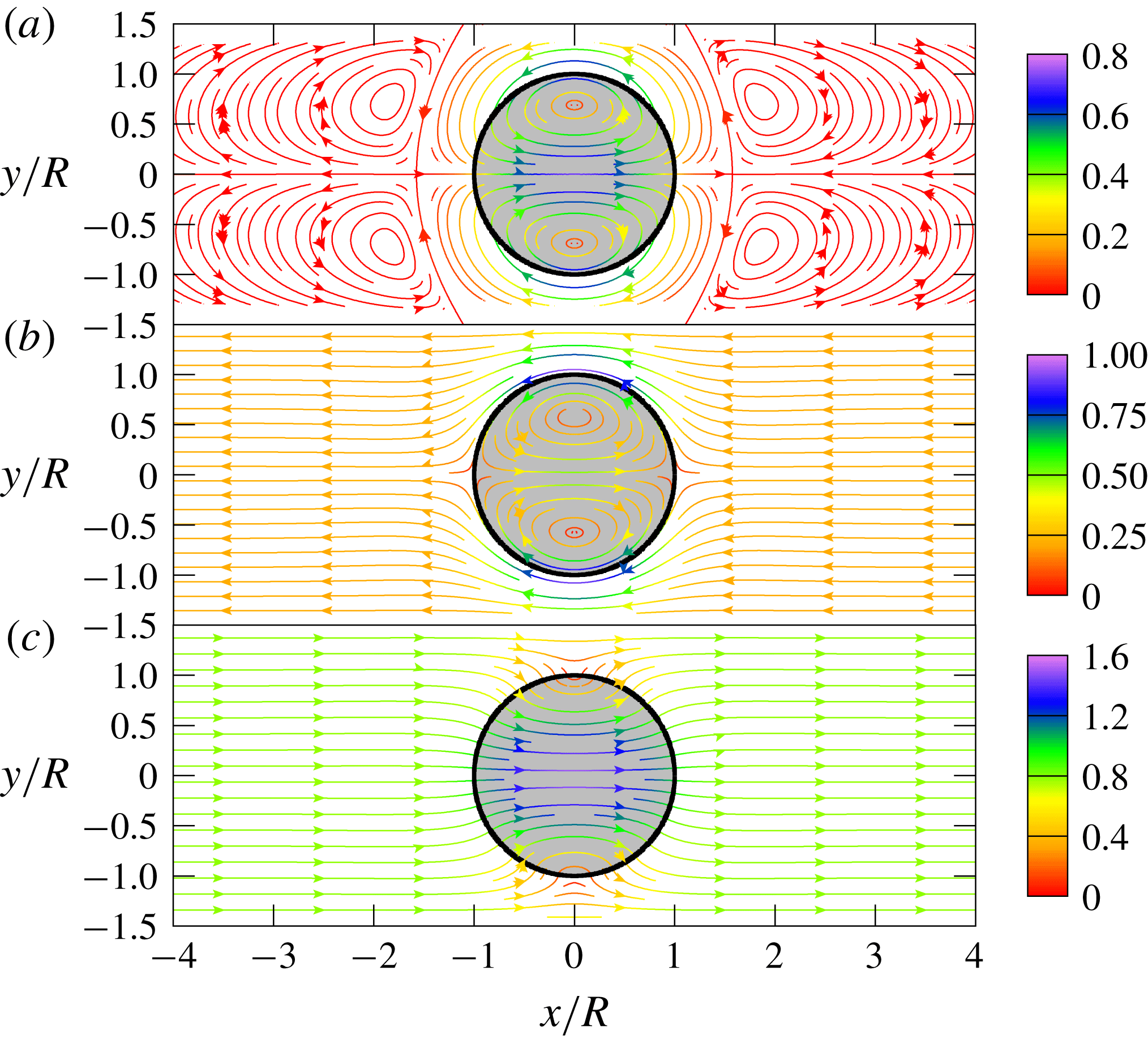
We highlight the link between the squirmer and pumper by drawing the flow lines for each swimmer. The flow lines in a channel were calculated from full numerical solution and are shown in figure 5. The flow is exactly the same for both swimmer types in the wall frame of reference (figure 5 a). The difference of the flow lines in the swimmer frame (figure 5 b,c) arises from the difference of the swimming speed for squirmer and pumper.
Flow lines around a confined circular swimmer. (a) Flow lines in the wall frame both for squirmer and pumper. (b) Flow lines in the swimmer frame for a squirmer. (c) Flow lines in the swimmer frame for a pumper. Numerical simulations. Swimmers are located in the centre of the channel with
 $W=3R$
.

6 Discussion
The main result of our analysis is (4.2) and (5.2) which presents the speeds of the amoeboid and squirmer swimmers as a function of the confinement. Interestingly, the only coefficient in (4.2) (amoeboid swimmer) that does not follow the same trend in term of amplitude is the one corresponding to
 $C_{n}^{2}$
. This smallness is a consequence of the almost perfect cancellation of the two contributions which make up this coefficient: the first one is due to the source dipole of the swimmer, which gets scattered off the walls, creating a flow opposite to the swimming direction. The second one is due to the stresslet of the swimmer, which creates a linear flow at the swimmer position when scattered off the walls. This linear flow modifies the swimming velocity by interacting with the deformations of the swimmer. The absence of this trend (smallness of the leading-order coefficient) for the squirmer is attributed to the absence of shape deformation.
The
 $C_{n}^{2}$
coefficient is negative for both swimmers, which means that
 $v_{s}$
decreases with increasing
 $C_{n}$
for small values of
 $C_{n}.$
However, since the coefficient of the
 $C_{n}^{2}$
is anomalously small for an amoeboid swimmer, the next term becomes dominant for
 $C_{n}$
much smaller than would otherwise be expected from the radius of convergence of (4.2). The
 $C_{n}^{4}$
coefficient in (4.2) is positive, which means that
 $\unicode[STIX]{x0394}X$
increases with
 $C_{n}$
for moderate confinements. We find that the minimum of
 $\unicode[STIX]{x0394}X$
occurs at
 $C_{n}=0.1048$
. Numerical simulations (Wu et al.
Reference Wu, Thiébaud, Hu, Farutin, Rafaï, Lai, Peyla and Misbah2015, Reference Wu, Farutin, Hu, Thiebaud, Rafai, Peyla, Lai and Misbah2016) show that
 $\unicode[STIX]{x0394}X$
goes through a maximum for high values of
 $C_{n}$
and starts decreasing with increasing
 $C_{n}.$
This region of parameters, however, is beyond the radius of convergence of (4.2) and thus cannot be analysed with the present calculation. Furthermore, the numerical simulations (Wu et al.
Reference Wu, Thiébaud, Hu, Farutin, Rafaï, Lai, Peyla and Misbah2015, Reference Wu, Farutin, Hu, Thiebaud, Rafai, Peyla, Lai and Misbah2016) were performed for large but finite values of the saturation number
 $S$
. The approximation of fully saturated strokes becomes inadequate for strongly confined swimmers because of the slowdown of the lubrication dynamics as the gaps between the swimmer and the walls are narrow enough. Eventually, the channel becomes too narrow for the deformation amplitudes attained in fully saturated regime to be possible to deploy. The situation is different for the squirmer (or pumper) since the leading term in
 $C_{n}^{2}$
dominates causing the squirmer (pumper) to be monotonous.
The fact that the leading-order term is negative for the amoeboid swimmer and squirmer can be intuitively understood as follows. In order to move forward, the swimmer has to drag fluid from front to rear, and the presence of walls makes this operation more difficult, leading to a decrease of speed. The amoeboid swimmer has the ability to adapt its shape to reflection of the flow on the wall, taking advantage of its deformation to increase the gap between its shape and the wall. We believe that this is the source of the smallness of the
 $C_{n}^{2}$
coefficient. The pumper pumps fluid from the front to the rear so that it can drag the fluid through its body rather than on the side. The existence of a pumping alternative may be the reason for the increase of its velocity with confinement.
The present study uses a two-dimensional model of the swimmer. Nevertheless, some of the results can be expected to remain valid in three dimensions. The hydrodynamic interactions have a faster decay rate in three dimensions than in two dimensions: the flow field due to a point force depends as
 $1/r$
in three dimensions and as
 $\ln r$
in two dimensions on the distance
 $r$
from the origin of the force. Thus, the flow field due to a force dipole decays as
 $1/r^{2}$
in three dimensions, while the flow field of a force quadrupole (equivalent to source dipole) decays as
 $1/r^{3}$
. This suggests that the leading effect of confinement would be characterized by a term of order
 $O(C_{n}^{3})$
both for a tube and for a slit geometry.
Similarly to the two-dimensional case, the leading-order contribution of the confinement to the swimming velocity comes from two sources: the effect of the source dipole of the swimmer scattered off the walls and the linear flow at the swimmer position, which is created by the stresslet of the swimmer scattered off the walls. The coefficients with which these two effects enter the swimming velocity depend on the geometry of the confinement. A detailed analysis in three dimensions represents an important question for further research.
Acknowledgements
We thank CNES (Centre National d’Etudes Spatiales), ESA (European Space Agency), and the French–German university program ‘Living Fluids’ (grant CFDA-Q1-14). The simulations were performed on the Cactus cluster of the CIMENT infrastructure, which is supported by the Rhône-Alpes region (GRANT CPER07_13 CIRA).
Appendix A. Flow representation
Let us introduce a potential function
 $\unicode[STIX]{x1D6EC}(z,z^{\ast },t)$
to be related to the complex velocity field
 $\hat{u}$
. The divergence-free condition
 $\unicode[STIX]{x1D735}\boldsymbol{\cdot }\boldsymbol{u}=0$
can be satisfied by introducing a real-valued scalar potential
 $\unicode[STIX]{x1D6EC}(z,z^{\ast },t)$
, related to the velocity field
 $\hat{u}$
as
 $$\begin{eqnarray}\hat{u} =\frac{\unicode[STIX]{x2202}\unicode[STIX]{x1D6EC}}{\unicode[STIX]{x2202}y}-\text{i}\frac{\unicode[STIX]{x2202}\unicode[STIX]{x1D6EC}}{\unicode[STIX]{x2202}x}.\end{eqnarray}$$
Taking the curl of the first equation (2.2) entails that
 $\unicode[STIX]{x1D6EC}$
is a biharmonic function
 $$\begin{eqnarray}\unicode[STIX]{x1D6FB}^{4}\unicode[STIX]{x1D6EC}=0.\end{eqnarray}$$
Upon using the relations between
 $x,y$
and
 $z,z^{\ast }$
one obtains that this equation transforms into
 $$\begin{eqnarray}\frac{\unicode[STIX]{x2202}^{4}\unicode[STIX]{x1D6EC}}{\unicode[STIX]{x2202}z^{2}\unicode[STIX]{x2202}{z^{\ast }}^{2}}=0.\end{eqnarray}$$
The general solution of which is
 $$\begin{eqnarray}2\unicode[STIX]{x1D6EC}(z,z^{\ast })=f(z)+f_{1}(z^{\ast })+z^{\ast }g(z)+zg_{1}(z^{\ast }),\end{eqnarray}$$
where the four functions on the right-hand side are arbitrary analytic functions of their respective complex argument (the factor 2 on the left-hand side is introduced for practical purposes). It is necessary that
 $g_{1}(z^{\ast })=(g(z))^{\ast }$
and
 $f_{1}(z^{\ast })=(f(z))^{\ast }$
in order to guarantee that
 $\unicode[STIX]{x1D6EC}$
is a real-valued function. This allows us to write finally that
 $$\begin{eqnarray}\unicode[STIX]{x1D6EC}(z,z^{\ast })=\text{Re}[f(z)+z^{\ast }g(z)].\end{eqnarray}$$
The velocity field can then be written as
 $$\begin{eqnarray}\hat{u} =-2\text{i}\frac{\unicode[STIX]{x2202}\unicode[STIX]{x1D6EC}}{\unicode[STIX]{x2202}z^{\ast }}=-2\text{i}[g(z)+f{(z)^{\ast }}^{\prime }+zg{(z)^{\ast }}^{\prime }]\equiv A(z)-zA^{\prime }(z)^{\ast }+B(z)^{\ast },\end{eqnarray}$$
where
 $A$
and
 $B$
are two analytic functions obviously related to
 $f$
and
 $g$
.