INTRODUCTION
The Cordilleran Ice Sheet (CIS) repeatedly covered the mountainous regions of western North America during the Pleistocene and formed part of the North American Ice Sheet Complex during the last glacial maximum (LGM). The CIS had an ice volume sea level equivalent of 7–9 m (Seguinot et al., Reference Seguinot, Rogozhina, Stroeven, Margold and Kleman2016), which is similar to the present-day Greenland Ice Sheet. Recent studies indicate that the CIS underwent substantial ice mass loss during the Bølling warming, after which the last stage of deglaciation is largely unknown (Peltier et al., Reference Peltier, Argus and Drummond2015; Lambeck at al., Reference Lambeck, Purcell and Zhao2017; Menounos et al., Reference Menounos, Goehring, Osborn, Margold, Ward, Bond and Clarke2017). This makes the CIS one of the least understood ephemeral Pleistocene ice sheets.
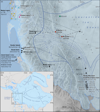
The interaction between the Cordilleran and Laurentide ice sheets east of the Rocky Mountains at the LGM has been debated for many decades, with some researchers arguing for the coalescence of the two ice sheets on the westernmost Interior Plains (e.g., Mathews, Reference Mathews1978; Dyke and Prest, Reference Dyke and Prest1987; Stumpf et al., Reference Stumpf, Broster and Levson2000; Dyke et al., Reference Dyke, Moore and Robertson2003; Dyke, Reference Dyke, Ehlers and Gibbard2004; Bednarski and Smith, Reference Bednarski and Smith2007), while others argue that the CIS did not extend over the Rocky Mountains at the local LGM (lLGM) (e.g., Bobrowsky and Rutter, Reference Bobrowsky and Rutter1992; Catto et al., Reference Catto, Liverman, Bobrowsky and Rutter1996). Recently, empirical evidence supporting the coalescence of the two ice sheets has grown (Atkinson et al., Reference Atkinson, Pawley and Utting2016; Hickin et al., Reference Hickin, Lian and Levson2016; Hartman et al., Reference Hartman, Clague, Barendregt and Reyes2018), and it is now generally accepted that they coalesced at the lLGM (Fig. 1). Recent studies based on glacial isostatic adjustment (GIA) analysis indicate substantial ice thickness in the area of coalescence, with an ice saddle connecting the dome areas of the two ice sheets (Peltier et al., Reference Peltier, Argus and Drummond2015; Lambeck at al., Reference Lambeck, Purcell and Zhao2017). However, the lLGM ice sheet configuration of the CIS is still not fully understood.
(a) Configuration of the Cordilleran Ice Sheet at 22.1 cal ka BP, based on Kleman et al. (Reference Kleman, Jansson, De Angelis, Stroeven, Hättestrand, Alm and Glasser2010), Margold et al. (Reference Margold, Stokes and Clark2018, Reference Margold, Gosse, Hidy, Woywitka, Young and Froese2019), and Dalton et al. (Reference Dalton, Margold, Stokes, Tarasov, Dyke, Adams and Allard2020). The approximate position of the ice divide at the lLGM is shown with thick blue lines; ice flow direction is indicated by thin blue lines. The locations of Mount Morfee and Mount Spieker are given by the red stars; remaining stars show the locations of selected 10Be cosmogenic nuclide ages relating to the deglaciation of the CIS from Margold et al. (Reference Margold, Stroeven, Clague and Heyman2014, Reference Margold, Gosse, Hidy, Woywitka, Young and Froese2019), Darvill et al. (Reference Darvill, Menounos, Goehring, Lian and Caffee2018), and Lesnek et al. (Reference Lesnek, Briner, Lindqvist, Baichtal and Heaton2018, Reference Lesnek, Briner, Baichtal and Lyles2020). All ages have been recalculated using the online calculator of Balco et al. (Reference Balco, Stone, Lifton and Dunai2008; version 3.0) and corrected for glacioisostatic rebound. The ages in bold also have been corrected for snow cover. All ages are given in thousands of years (ka) and are reported with a 1σ external error. In most cases the weighted mean age of a specific number of samples (n) is given. The green square gives the location of a 36Cl exposure age from Bednarski and Smith (Reference Bednarski and Smith2007) that has not been recalculated. The abbreviation PH shows the location of the Porcupine Hills. The location of the transect shown in Fig. 8 is given by the black dashed line B–B’. (b) Inset map of the North American Ice Sheet Complex showing the location of the Cordilleran Ice Sheet and the ice extent at 22.1 cal ka BP. The approximate positions of the ice divides and ice domes are shown by the thick blue lines (K = Keewatin dome, Q-L = Québec-Labrador dome, F-B = Foxe-Baffin dome; Margold et al., Reference Margold, Stokes and Clark2018). (For interpretation of the references to color in this figure legend, the reader is referred to the web version of this article.)

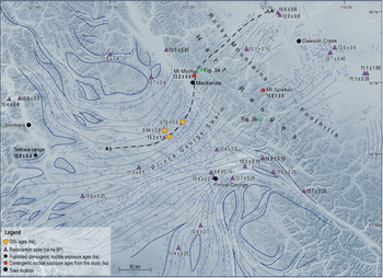
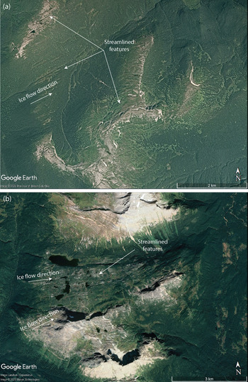
Empirical evidence indicates that ice flowed over the Rocky Mountains at the Hart Ranges (Fig. 2), the lowest and least rugged section of the mountain range (summits averaging 2300 m above sea level [asl]). This evidence includes (1) sets of attenuated bedforms on either side of the Hart Ranges, which record fast ice flow towards the Rocky Mountains (Prince George swarm; Kleman et al., Reference Kleman, Jansson, De Angelis, Stroeven, Hättestrand, Alm and Glasser2010; Sacco et al., Reference Sacco, Ward, Lian, Maynard and Geertsema2017) and fast ice flow radiating from the Rocky Mountain Foothills (Fig. 2; Prest et al., Reference Prest, Grant and Rampton1968; Kleman et al., Reference Kleman, Jansson, De Angelis, Stroeven, Hättestrand, Alm and Glasser2010; Shaw et al., Reference Shaw, Sharpe and Harris2010; Atkinson et al., Reference Atkinson, Pawley and Utting2016; Hickin et al., Reference Hickin, Lian and Levson2016), (2) northeast-trending streamlined landforms on mountain summits between 55°N and 56°N (Fig. 3a), (3) geomorphological evidence of ice drainage through a system of broad mountain cols located between 54.5°N and 55°N (Fig. 3b), (4) eastwardly transported glacial erratics along the Rocky Mountain Foothills (Bednarski and Smith, Reference Bednarski and Smith2007), and (5) the presence of volcanic-rich Cordilleran till east of the Rocky Mountains (Mathews, Reference Mathews1978; Bednarski and Smith, Reference Bednarski and Smith2007; Hartman et al., Reference Hartman, Clague, Barendregt and Reyes2018).
Regional map of the ice flow surrounding the Hart Ranges. The thin blue lines represent the empirical ice flow evidence (drumlins and crag and tails) mapped by Shaw et al. (Reference Shaw, Sharpe and Harris2010); the continuous, thick blue lines show the ice flow pattern interpreted by Kleman et al. (Reference Kleman, Jansson, De Angelis, Stroeven, Hättestrand, Alm and Glasser2010). Purple triangles show the median calibrated radiocarbon ages in cal ka BP surrounding the Hart Ranges from Dalton et al. (Reference Dalton, Margold, Stokes, Tarasov, Dyke, Adams and Allard2020). The orange hexagons show the optically stimulated luminescence ages from Sacco et al. (Reference Sacco, Ward, Lian, Maynard and Geertsema2017). The locations of the two study sites are shown by the red stars with their weighted-mean exposure ages. The location of Figure 3a and 3b is shown by the green circles. The location of the ice surface profile shown in Figure 7 is given by the black dashed line A–A’. (For interpretation of the references to color in this figure legend, the reader is referred to the web version of this article.)

(color online) Google Earth images of (a) the streamlined features observed on some of the mountain peaks in the Hart Ranges of the Rocky Mountains with a maximum elevation of 1780 m asl and (b) evidence of ice flow through a broad mountain col in the Hart Ranges at an elevation of 1500 m asl. The locations of these figures are shown in Figure 2.

Margold et al. (Reference Margold, Stokes and Clark2018, Reference Margold, Gosse, Hidy, Woywitka, Young and Froese2019) incorporated ice flow over the Hart Ranges into a broader, regional picture of the ice sheet configuration, showing the ice drainage pattern at, and shortly after, the lLGM. According to their reconstructions, which integrated data on the glacial geomorphology (Margold et al., Reference Margold, Stokes, Clark and Kleman2015a, Reference Margold, Stokes and Clarkb) with information from glacial isostasy (Peltier, Reference Peltier2004; Peltier et al., Reference Peltier, Argus and Drummond2015, Lambeck et al., Reference Lambeck, Purcell and Zhao2017) and numerical ice sheet modelling (Tarasov and Peltier, Reference Tarasov and Peltier2004; Tarasov et al., Reference Tarasov, Dyke, Neal and Peltier2012), an ice saddle connecting the CIS and Laurentide Ice Sheet (LIS) was located east of the Rocky Mountains at the lLGM. Cordilleran ice flowed over the Rocky Mountains and into the Rocky Mountain Foothills Ice Stream, a tributary of an anastomosing ice stream system draining the Keewatin ice dome of the LIS at the lLGM (Fig. 1).
Ice flow over the Rocky Mountains has thus far remained unconstrained in time, with the lLGM being defined by sub-till radiocarbon ages along the marine-terminating margin (e.g., Clague, et al., Reference Clague, Armstrong and Mathews1980; Blaise et al., Reference Blaise, Clague and Mathewes1990; Ward et al., Reference Ward, Wilson, Nagorsen, Nelson, Driver and Wigen2003; Al-Suwaidi et al., Reference Al-Suwaidi, Ward, Wilson, Hebda, Nagorsen, Marshall, Ghaleb, Wigen and Enkin2006) and by the timing of the early stages of ice retreat along the ice sheet perimeter (Stroeven et al., Reference Stroeven, Fabel, Codilean, Kleman, Clague, Miguens-Rodriguez and Xu2010, Reference Stroeven, Fabel, Margold, Clague and Xu2014; Darvill et al., Reference Darvill, Menounos, Goehring, Lian and Caffee2018; Lesnek et al., Reference Lesnek, Briner, Lindqvist, Baichtal and Heaton2018, Reference Lesnek, Briner, Baichtal and Lyles2020; Margold et al., Reference Margold, Gosse, Hidy, Woywitka, Young and Froese2019). Here we use in situ produced cosmogenic 10Be dating on glacial erratic boulders located on two summit peaks on opposite sides of the Hart Ranges of the Rocky Mountains to determine when Cordilleran ice stopped flowing over the mountain range.
METHODS
Boulder surface sampling
Glacial erratics located on mountain summits that contain geomorphological evidence of ice flow (e.g., streamlined landforms) were examined (Fig. 3a) and two sites that are accessible by foot were chosen for sampling: one site on the western side (Mount Morfee, 1660 m asl) and one site on the eastern side of the Hart Ranges (Mount Spieker, 1971 m asl). Four boulders were sampled at each location in order to minimize the impact of choosing a sample with a complex exposure history. Additionally, where possible, erratics with a different lithology to the surrounding bedrock were targeted in order to minimize the chance of cosmogenic nuclide inheritance (Heyman et al., Reference Heyman, Stroeven, Harbor and Caffee2011).
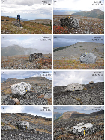
Samples from Mount Morfee (RM18-01 to RM18-04) were collected on a flattish, glacially eroded western secondary summit (main summit elevation 1775 m asl) that is situated right at the western mountain front of the Hart Ranges. Sample RM18-01 was collected on the slope west of the secondary summit, samples RM18-02 and RM18-03 were collected directly on the secondary summit, and sample RM18-04 on a col between the secondary summit and the main summit of Mount Morfee (see Fig. 4a-d).
(color online) Photographs of the sampled boulders presented with their apparent exposure ages ± 1σ external error. (a–d) Boulders RM18-01 to RM18-04 that are located at Mount Morfee. (e–h) Boulders RM18-05 to RM18-08 that are located at Mount Spieker. Boulder RM18-06 is considered an outlier. Note the person and chisel for scale.

Mount Spieker has a flat, elongated summit surface bordered by steep headwalls of large cirques in all directions. We collected samples RM18-05 to RM18-08 on this summit surface. The boulders from which we collected samples RM18-05 and RM18-06 were situated 60 m and 100 m, respectively, from the eastern rim of the summit, and the boulders of samples RM18-07 and RM18-08 were situated an equal distance between the western and eastern rim of the summit surface. All of the Mount Spieker boulders were perched on the bedrock (see Fig. 4e–h).
Samples were collected from the top surface of the erratics with a hammer and chisel. Sample locations and elevations were marked with a handheld GPS (~4 m horizontal accuracy), and a clinometer was used to measure the topographic shielding. The selected boulders showed no evidence of denudation and were not covered by moss or other vegetation. In addition, at Mount Morfee, we collected ~30 well-rounded cobbles of glacial drift that littered the surface to determine their provenance in order to test the hypothesis that ice flowed in an easterly direction across the western mountain front.
Sample preparation and AMS measurements
Measuring the 10Be concentration in quartz requires several purification steps before the sample can be brought to the accelerator mass spectrometer (AMS) to measure its 10Be/9Be ratio (Gosse and Phillips, Reference Gosse and Phillips2001). The samples were crushed, sieved, and cleaned with a mixture of HCl and H2SiF6. A weighed amount (~ 0.1 g) of a 3025 ± 9 ppm 9Be solution of was added as a carrier to the decontaminated quartz. Beryllium was separated from the solution by successive anionic and cationic resin extractions and precipitations. The final precipitates were dried, heated to 800°C to obtain BeO, and mixed with niobium powder. The 10Be/9Be ratio of each sample was measured at the French 5 MV AMS National Facility ASTER (CEREGE, Aix-en-Provence). The measurements were calibrated directly against STD11 inhouse standard (10Be/9Be value of 1.191 ± 0.013 × 10⁻¹¹; Braucher et al., Reference Braucher, Guillou, Bourlès, Arnold, Aumaître, Keddadouche and Nottoli2015). A process blank was also analyzed and used to subtract 10Be introduced during target preparation and analysis. This blank (10Be/9Be = 2.65 ± 0.36 × 10⁻¹⁵) accounts at maximum for 1.6% of the measured ratios.
10Be age calculations
The exposure ages were calculated using the online calculator of Balco et al. (Reference Balco, Stone, Lifton and Dunai2008; version 3.0), with the ‘primary’ calibration set of Borchers et al. (Reference Borchers, Marrero, Balco, Caffee, Goehring, Lifton, Nishiizumi, Phillips, Schaefer and Stone2016). The ages are reported here using the time-dependent CRONUS LSDn production rate scaling model (Lifton et al., Reference Lifton, Sato and Dunai2014). Individual ages are reported with an external error (reported as 1σ), which accounts for both measurement uncertainties, including uncertainties associated with AMS counting statistics, chemical blank measurements, and AMS internal error (0.5%), as well as uncertainties in the reference nuclide production rate for spallation and the nuclide production rate by muons (Balco et al., Reference Balco, Stone, Lifton and Dunai2008). At each site, a weighted mean exposure age was calculated and reported with a weighted mean standard deviation. A chi-squared (χ2) test was used to examine the distribution of exposure ages at each site (Ward and Wilson, Reference Ward and Wilson1978). The 95% critical value for χ2 with n-1 degrees of freedom was calculated for each site and compared with the theoretical value (χ2crit; supplementary material D4). If the calculated value was less than the theoretical value, all ages were used to calculate the mean exposure age. However, if the site did not pass this test, the ages with the largest calculated χ2 value were successively excluded until the distribution passed the χ2 test (Dunai, Reference Dunai2010). Additionally, following the procedure presented by Blomdin et al. (Reference Blomdin, Stroeven, Harbor, Lifton, Heyman, Gribenski and Petrakov2016), the reduced chi-squared statistic and the standard deviation to arithmetic mean exposure age ratio was used to determine the approximate scatter in the data and classify the sites as well, moderately, or poorly clustered (see supplementary material D4).
Processes affecting terrestrial cosmogenic nuclide production rates
A number of processes can affect terrestrial cosmogenic nuclide production rates, including boulder surface denudation, snow and vegetation cover, elevation changes from GIA, and variations in the atmospheric mass distribution over time (Gosse and Phillips, Reference Gosse and Phillips2001; Jones et al., Reference Jones, Whitehorse, Bentley and Dalton2019). There is currently no universal method for addressing and accounting for these processes, and we assessed the effect of each process at our sample sites individually.
We did not correct the apparent exposure ages for surface denudation because most of the boulders consist of highly resistant rocks. The Rocky Mountain range creates a marked topographic barrier to the prevailing westerly winds, causing significant present-day snow cover to occur for eight months of the year at both sample sites. The average snow depth per month exceeds the height of all boulders, therefore, we applied a snow shielding correction to the apparent exposure ages. This snow shielding factor was calculated at each site for each month of the year (monthly snow depth and density data was obtained from nearby manual weather stations; see supplementary material S1; Government of Canada, 2019) and averaged to give an annual snow shielding factor for each sample. The snow depth was calculated individually for each boulder by subtracting the boulder height from the monthly snow depth. The snow shielding factor was then calculated according to the exponential attenuation equation for snow shielding presented in Gosse and Phillips (Reference Gosse and Phillips2001, equation 3.76; see supplementary material S1).
The monthly snow depth and density data provide a reasonably good estimate of the present-day snow cover at each site because the data are available over a 50 year period and the weather stations are located at similar elevations and within 50 km of the sample sites. However, our snow cover correction does not account for long term changes in climate over the Holocene, such as the early Holocene thermal maximum (ca. 11.5–8.0 ka) when temperatures were ~2–4°C warmer than present in western Canada (Pellatt and Mathewes, Reference Pellatt and Mathewes1997; Edwards et al., Reference Edwards, Birks, Luckman and MacDonald2008; Gavin et al., Reference Gavin, Henderson, Westover, Fritz, Walker, Leng and Hu2011; Schwörer et al., Reference Schwörer, Gavin, Walker and Hu2017). This variation in climate introduces a large uncertainty into our snow cover corrected apparent exposure ages.
The LSDn production rate scaling model was used to determine the specific 10Be production rate at each of our sample sites as a function of altitude (atmospheric pressure) and latitude. This scaling model assumes that the atmospheric pressure has remained constant over time. However, at our sample sites, atmospheric pressure has varied due to (1) changes in altitude caused by GIA; and (2) changes in the atmospheric density distribution during the glacial-interglacial cycle due to a range of processes, such as the displacement of atmospheric mass, katabatic winds, and atmospheric cooling (Staiger et al., Reference Staiger, Gosse, Toracinta, Oglesby, Fastook and Johnson2007; Jones et al., Reference Jones, Whitehorse, Bentley and Dalton2019). It has been hypothesized that the changes in atmospheric pressure due to GIA might be offset to some degree by the changes in the atmospheric density distribution caused by changes in the climate over time (Staiger et al., Reference Staiger, Gosse, Toracinta, Oglesby, Fastook and Johnson2007; Young et al., Reference Young, Schaefer, Briner and Goehring2013), and there has recently been some debate about our ability to properly account for these changes (e.g., Staiger et al., Reference Staiger, Gosse, Toracinta, Oglesby, Fastook and Johnson2007; Jones et al., Reference Jones, Whitehorse, Bentley and Dalton2019; Balco, Reference Balco2020). Here we assess both the time-varying effects of GIA and the changing atmospheric thickness on the 10Be production rate at our sites since deglaciation.
We used the published relative sea level change (ΔRSL) data from Lambeck et al. (Reference Lambeck, Purcell and Zhao2017; currently the highest resolution GIA model available with a 0.25 x 0.25° resolution and 500 year intervals) to determine the average elevation of the sample sites since deglaciation. According to their model, the Mount Morfee and Mount Spieker sites became ice free at 13.0 ka and 13.5 ka, respectively. Therefore, we extracted the ΔRSL value every 500 years since the deglaciation and then calculated the average ΔRSL for the entire period, which results in a change of -62 m at Mount Morfee and -64 m at Mount Spieker (see supplementary material D2). We then corrected the modern elevation of the sample sites by this value before the exposure ages were calculated.
We used the method developed by Cuzzone et al. (Reference Cuzzone, Clark, Carlson, Ullman, Rinterknecht, Milne, Lunkka, Wohlfarth, Marcott and Caffee2016) for assessing the effect of changing atmospheric thickness on production rates. This method uses the hypsometric equation to calculate the change in atmospheric thickness (m) between the time of deglaciation and the present-day. Simulated variations in surface pressure over time at our field sites and the average temperature since deglaciation were obtained from the output of a coupled atmosphere-ocean general circulation model (simulating global climate at 3 ka time intervals over the last 21 ka; Alder and Hostetler, Reference Alder and Hostetler2015) and used in the hypsometric equation. Although the temporal (3 ka) and spatial (3.75° x 3.68°) resolution of this model is rather coarse compared with the GIA model, the calculation indicates that the change in elevation due to variations in atmospheric density distribution between 15–0 ka is 3.4 m. This result is consistent with that of Cuzzone et al. (Reference Cuzzone, Clark, Carlson, Ullman, Rinterknecht, Milne, Lunkka, Wohlfarth, Marcott and Caffee2016) and Ullman et al. (Reference Ullman, Carlson, Hostetler, Clark, Cuzzone, Milne, Winsor and Caffee2016), who found that although this correction works in the opposite direction to that of the GIA correction, it is an order of magnitude smaller, and therefore, we excluded it from our overall topographic correction and only account of changes due to GIA.
Recalculating previously published 10Be ages
All previously published 10Be ages presented in this paper have been recalculated with the online calculator to ensure they are directly comparable (see supplementary material D3). Where multiple ages are available for a particular site, a weighted mean age has been calculated (excluding outliers identified by the original authors). A snow cover correction was applied only at the Telkwa Range because all the other sites do not receive enough snow cover to require corrections to their exposure ages. A GIA correction was applied to all ages using the method outlined above. The majority of these recalculated ages are younger than the previously published ages; this is coming from the time-dependent CRONUS LSDn production rate scaling scheme.
RESULTS
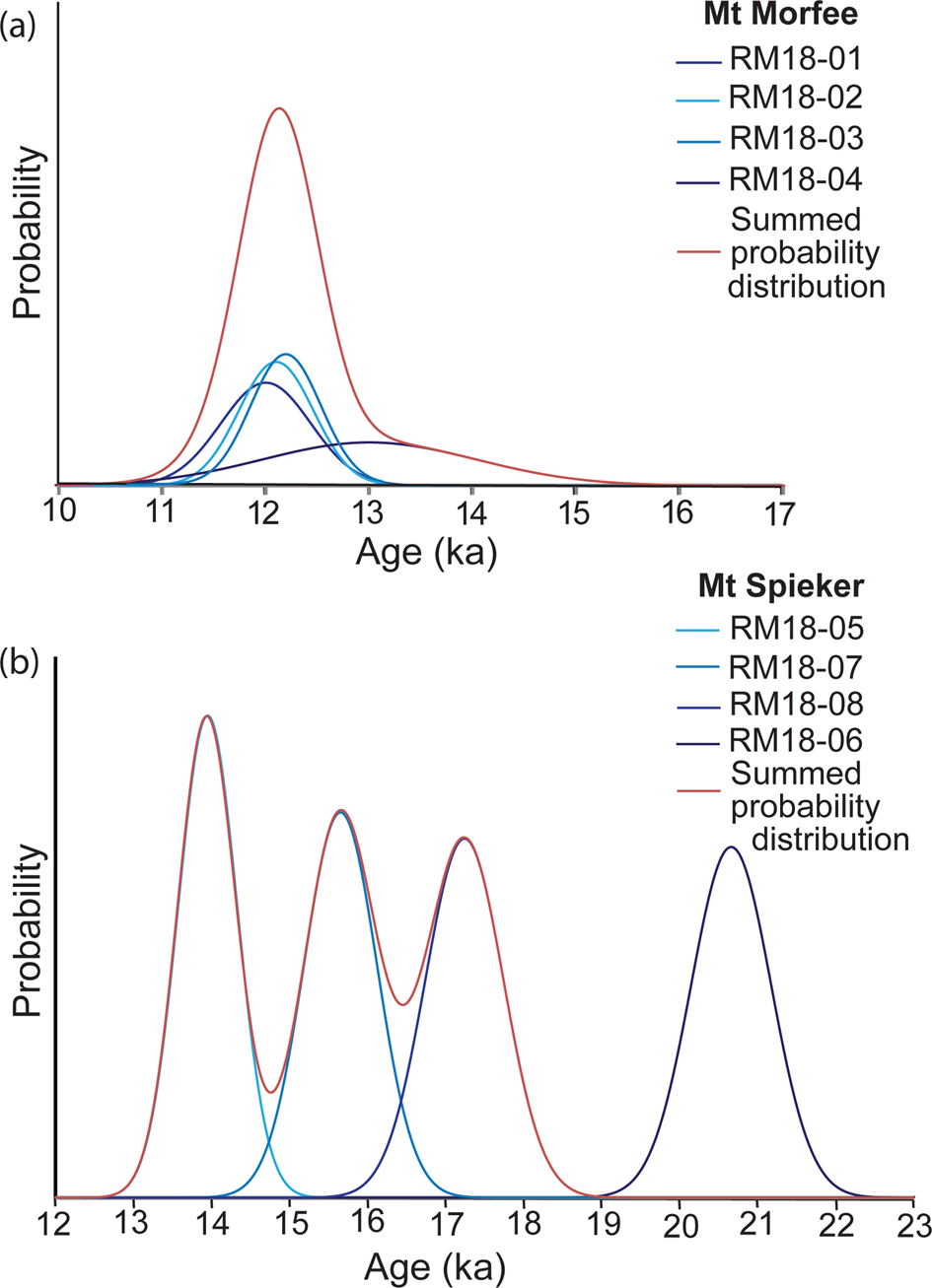
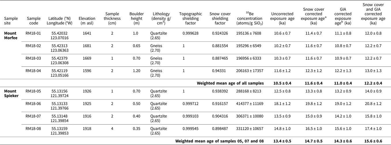
The 10Be exposure ages of each sample are given in Table 1. The four exposure ages obtained from Mount Morfee are well clustered between 12.0 ± 0.8 ka and 13.0 ± 1.3 ka, with a weighted mean age and weighted mean standard deviation of 12.2 ± 0.4 ka (Fig. 5A). At Mount Spieker, sample number RM18-06, with an exposure age of 20.8 ± 1.2 ka, was identified as an outlier and excluded from the weighted mean exposure age calculation for the site based on the results of the χ2 calculation (see supplementary material D4). The remaining three samples give moderately clustered exposure ages between 14.0 ± 0.9 ka and 17.4 ± 1.0 ka, with a weighted mean exposure age and weighted mean standard deviation of 15.6 ± 0.6 ka (Fig. 5B).
(color online) Probability distributions for the apparent exposure ages at (a) Mount Morfee and (b) Mount Spieker. At Mount Spieker, sample RM18-06 has been omitted from the summed probability distribution.

Location and description of the samples collected at Mount Morfee and Mount Spieker during this study. The uncorrected and snow cover and GIA corrected surface exposure ages are given for the individual samples RM18-01 to RM18-08 as well as the calculated weighted mean exposure age for each sample site. Only the snow cover and GIA corrected exposure ages are referred to in the text.

a The snow cover correction makes the ages 6.0–13.7% older.
b The GIA correction makes the ages 4.7–5.8% older.
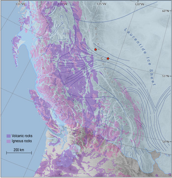
A number of the cobbles collected from the till at Mount Morfee originated from felsic and mafic intrusive and extrusive rocks, with the following lithologies identified: rhyolite with alkali feldspar, dacite, tonalite, alkali feldspar granite, gabbro, and basalt. Because the Rocky Mountains and Alberta Plateau (Canadian Prairies) both consist of sedimentary bedrock, these volcanic cobbles were almost certainly sourced from the Northern Cordilleran Volcanic Province, which extends in a north-northwest direction across central British Columbia (Fig. 6). The western provenance of these volcanic cobbles confirms the easterly flow of Cordilleran ice over the Hart Ranges.
Distribution of intrusive (pink) and extrusive (purple) igneous rocks across part of western North America, overlaid on the ice sheet extent at 22.1 cal ka BP based on the radiocarbon chronology of Dalton et al. (Reference Dalton, Margold, Stokes, Tarasov, Dyke, Adams and Allard2020). The approximate position of the ice divide at the lLGM is shown with thick blue lines; ice flow direction is indicated by thin blue lines (Kleman et al., Reference Kleman, Jansson, De Angelis, Stroeven, Hättestrand, Alm and Glasser2010; Margold et al., Reference Margold, Stokes and Clark2018, Reference Margold, Gosse, Hidy, Woywitka, Young and Froese2019). In the south, the lLGM occurred later than 22.1 cal ka BP, therefore, the maximum ice extent is not shown here. The red stars show the locations of the Mount Spieker and Mount Morfee field sites. This map demonstrates that the volcanic and igneous rocks collected at Mount Morfee were sourced from the west, confirming the easterly ice flow direction over the Rocky Mountains. (For interpretation of the references to color in this figure legend, the reader is referred to the web version of this article.)

DISCUSSION
Interpreting the 10Be concentrations
A number of geomorphic processes can cause apparent exposure ages to differ from the true depositional age of a landform (Balco, Reference Balco2020), and the two main sources of geological uncertainty are nuclide inheritance and incomplete exposure (Heyman et al., Reference Heyman, Stroeven, Harbor and Caffee2011). Incomplete exposure results from post-depositional shielding of the sample due to burial and successive exhumation, which causes the apparent exposure age to be younger than the true depositional age. However, we consider it unlikely that the boulders sampled during this study were affected by incomplete exposure because at Mount Morfee, the boulders are too tall to be buried by sediment following deposition (0.65–1.20 m tall), and the majority of boulders at Mount Spieker are resting directly on bedrock.
The four ages from Mount Morfee are well clustered between 12.0 ± 0.8 ka and 13.0 ± 1.3 ka and, therefore, it is unlikely that nuclide inheritance affected the measured 10Be concentrations within these samples. In contrast, the four exposure ages from Mount Spieker show a larger spread in apparent exposure ages, between 14.0 ± 0.9 ka and 20.8 ± 1.2 ka. It is likely that nuclide inheritance affected the oldest measured sample, RM18-06, because the apparent exposure age of 20.8 ± 1.2 ka is in conflict with the surrounding deglaciation chronology (e.g., Margold et al., Reference Margold, Gosse, Hidy, Woywitka, Young and Froese2019; Dalton et al., Reference Dalton, Margold, Stokes, Tarasov, Dyke, Adams and Allard2020; Fig. 1). Consequently, this sample is considered an outlier and has been excluded from the weighted mean calculation at Mount Spieker. The remaining three samples are moderately clustered according to the criterion of Blomdin et al. (Reference Blomdin, Stroeven, Harbor, Lifton, Heyman, Gribenski and Petrakov2016).
Comparison of the exposure ages with regional deglaciation data
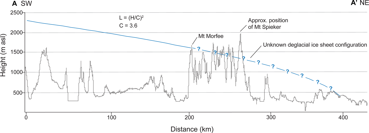
The coalescence of the CIS and LIS east of the Rocky Mountains is now well established (Atkinson et al., Reference Atkinson, Pawley and Utting2016; Hartman et al., Reference Hartman, Clague, Barendregt and Reyes2018; Margold et al., Reference Margold, Stokes and Clark2018), with this study providing further evidence for ice flow over the Rocky Mountains at the lLGM. In contrast, the timing and style of deglaciation in the interior of the ice sheet is very poorly constrained with the mountainous topography thus far impeding the reconstruction of ice sheet-wide glacial retreat patterns. Regionally, deglaciation of the CIS is often characterized by early emergence of mountain peaks due to downwasting and stagnation of ice in valleys (Fulton, Reference Fulton1967, Reference Fulton1991), however, in some areas, active ice retreat occurred during deglaciation, with active ice retreat of outlet glaciers documented in the Northern Rocky Mountain Foothills (Atkinson et al., Reference Atkinson, Pawley and Utting2016) and west of the Rocky Mountain Trench (Margold et al., Reference Margold, Jansson, Kleman, Stroeven and Clague2013; Sacco et al., Reference Sacco, Ward, Lian, Maynard and Geertsema2017). In the Rocky Mountains, the style and pattern of ice retreat is not well understood and may differ from other areas of the CIS because the mountain range forms a pronounced topographic barrier perpendicular to ice flow. While it is likely that the mountain summits of Mount Morfee and Mount Spieker emerged from the ice sheet ahead of the retreating ice margin, the relationship between downwasting versus active ice margin retreat remains uncertain (Fig. 7).
Hypothetical ice surface profile of the CIS when the ice margin is located at Mount Morfee, created using the empirical formula derived by Ng et al. (Reference Ng, Barr and Clark2010). We used a length of 400 km that spans 200 km west of Mount Morfee to the approximate position of the ice divide (solid blue line) and 200 km east to an imaginary ice margin (dashed blue line). Using a C coefficient of 3.6, which is similar to the C coefficient of the present-day Greenland Ice Sheet (3.1), the resulting ice surface profile has a height of 1600 m at Mount Morfee. The ice surface profile has been drawn along the flowline A–A’ shown in Figure 2. (For interpretation of the references to color in this figure legend, the reader is referred to the web version of this article.)

The available 36Cl and 10Be exposure ages, optically stimulated luminescence (OSL) dates, and radiocarbon dates that relate to the timing of ice retreat across the Hart Ranges are shown in Figures 1 and 2. The timing of deglaciation at Mount Spieker (weighted mean exposure age of 15.6 ± 0.6 ka) is consistent with the age of the Foothills Erratics Train, a group of quartzite boulders scattered linearly along the eastern foothills of the Rocky Mountains (Fig. 1; Jackson et al., Reference Jackson, Phillips, Shimamura and Little1997; Margold et al., Reference Margold, Gosse, Hidy, Woywitka, Young and Froese2019). The deposition of the Foothills Erratics Train at 15.0 ± 0.3 ka (n = 12; Margold et al., Reference Margold, Gosse, Hidy, Woywitka, Young and Froese2019), immediately preceding the onset of the Bølling warming (14.6–12.9 ka; Rasmussen et al., Reference Rasmussen, Bigler, Blockley, Blunier, Buchardt, Clausen and Cvijanovic2014), marks the beginning of the separation of the Laurentide, Cordilleran, and local mountain ice masses ~700 km southeast of the Hart Ranges. However, erratics at elevations of ~1650 m asl in the Porcupine Hills (Fig. 1) brought by the last (LGM) ice advance (Jackson et al., Reference Jackson, Phillips and Little1999) indicate that significant ice surface lowering occurred prior to the deposition of the Foothills Erratics Train and the separation of the ice sheets. We therefore suggest that deglaciation at Mount Spieker could have occurred contemporaneously with the separation of the LIS and CIS farther south.
The weighted mean exposure age at Mount Morfee of 12.2 ± 0.4 ka indicates the CIS extended to the western front of the Rocky Mountains during the Younger Dryas (YD) stadial (12.9–11.7 ka; Rasmussen et al., Reference Rasmussen, Bigler, Blockley, Blunier, Buchardt, Clausen and Cvijanovic2014). This age broadly agrees with the ice-sheet-scale radiocarbon-based ice margin chronology of Dyke (Reference Dyke, Ehlers and Gibbard2004) and Dalton et al. (Reference Dalton, Margold, Stokes, Tarasov, Dyke, Adams and Allard2020), according to which the eastern margin of the Cordilleran Ice Sheet detached from the western front of the Hart Ranges at some point between 12.8 cal ka BP and 12.1 cal ka BP. The corrected apparent exposure ages are older than the majority of radiocarbon ages and OSL dates, located immediately west of the Rocky Mountains, with two exceptions highlighted in bold text in Figure 2. The youngest age (12.8 ± 0.15 cal ka BP, wood, lab. no. GSC-2964; Lowdon and Blake., Reference Lowdon and Blake1980) is from the upper Fraser River area that likely deglaciated earlier than the Interior Plateau to the northwest, which led to the formation of Glacial Lake Fraser (Clague, Reference Clague1987; Margold et al., Reference Margold, Jansson, Kleman, Stroeven and Clague2013).
There are very few cosmogenic nuclide exposure ages for the interior of the former ice sheet that directly date the deglaciation, with the majority of exposure ages presented by Menounos et al. (Reference Menounos, Goehring, Osborn, Margold, Ward, Bond and Clarke2017) for the central sector of the CIS corresponding to a late glacial readvance of smaller mountain glaciers rather than the deglaciation of the CIS. This readvance of cirque glaciers has also been identified in the southern Rocky Mountains (locally termed the Crowfoot Advance; Reasoner et al., Reference Reasoner, Osborn and Rutter1994; Menounos et al., Reference Menounos, Osborn, Clague and Luckman2009). However, although the weighted mean exposure age at Mount Morfee falls within the YD stadial, we infer that there is no connection to the regional mountain glacier readvance because there is no geomorphological evidence for it (e.g., readvance moraines) in the Hart Ranges and the sample site is located on a summit peak that does not contain cirques.
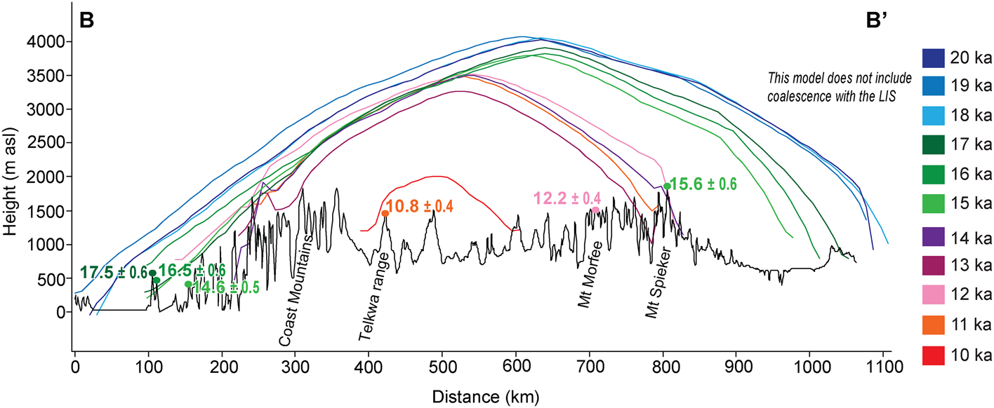
Figure 8 shows selected cosmogenic nuclide exposure ages along a west-east transect (shown in Fig. 1) and simulated ice surface profiles along the same transect from Seguinot et al. (Reference Seguinot, Rogozhina, Stroeven, Margold and Kleman2016) and Seguinot (Reference Seguinot2020). It can be seen that deglaciation at Mount Spieker occurred at roughly the same time as deglaciation along the Pacific Coast, with the ice margin retreating to the mainland coastline by ca. 14 ka (Darvill et al., Reference Darvill, Menounos, Goehring, Lian and Caffee2018; Lesnek et al., Reference Lesnek, Briner, Lindqvist, Baichtal and Heaton2018, Reference Lesnek, Briner, Baichtal and Lyles2020). The weighted mean age of 12.2 ± 0.4 ka at Mount Morfee then corresponds to a later stage of deglaciation, being only 1400 years older than that of the Telkwa Range (10.8 ± 0.4 ka; Margold et al., Reference Margold, Stroeven, Clague and Heyman2014), which was likely located close to the ice divide. Figure 8 also shows that the cosmogenic exposure ages along the transect broadly fit with the simulated thickness and extent of the CIS at 20–10 ka from the numerical model of Seguinot (Reference Seguinot2020). However, the GRIP ice core temperature data used to drive the Seguinot (Reference Seguinot2020) simulation induces a dramatic regrowth of the CIS due to the YD cooling, while the empirical evidence to support any such considerable advance is limited.
(color online) Simulated thickness and extent of the CIS from 20–10 ka from the numerical model of Seguinot (Reference Seguinot2020) using the GRIP ice core temperature forcing (note the pronounced YD regrowth of the ice sheet at 12 ka that might, at least partially, be an artefact of using the GRIP forcing). The location of the cross profile (B–B’) is shown in Figure 1. This cross profile passes through exposure age sample sites at Calvert and King Island (Darvill et al., Reference Darvill, Menounos, Goehring, Lian and Caffee2018), Telkwa range (Margold et al., Reference Margold, Stroeven, Clague and Heyman2014), Mount Morfee (this study), and Mount Spieker (this study). The weighted mean exposure ages from these studies are plotted in their approximate position along the elevation transect.

While our corrected apparent exposure ages from Mount Morfee and Mount Spieker generally fit the surrounding published numerical ages, our poor understanding of the deglacial ice sheet configuration over the Rocky Mountains means our exposure ages cannot be used to constrain the timing of the ice saddle collapse or opening of the ice free corridor east of the Rocky Mountains. However, regardless of the deglaciation style, our exposure ages indicate that the CIS still had a considerable extent during the YD with a surface elevation at the ice divide possibly reaching over 2000 m (Fig. 7). This finding conflicts with the GIA-based ice thickness models of Lambeck et al. (Reference Lambeck, Purcell and Zhao2017) and Peltier et al. (Reference Peltier, Argus and Drummond2015), which indicate deglaciation of the Hart Ranges ca. 13.0 ka after the CIS underwent substantial melting, losing up to half its mass, during the Bølling warming (Menounos et al., Reference Menounos, Goehring, Osborn, Margold, Ward, Bond and Clarke2017). A recent paper by Pico et al. (Reference Pico, Mitrovica and Mix2020), based on gravitationally self-consistent sea level simulations made to fit sea level records over the Bering Strait, has suggested that this meltwater flux instead happened during the YD stadial (13–11.5 ka).
We therefore suggest that further efforts combining paleoglaciological reconstructions, based on geomorphological mapping, with numerical dating are needed to understand the deglaciation of the central sector of the CIS and to explain the discrepancy between the numerical ages and ice thickness models. This will allow us to constrain the timing and style of deglaciation in the interior of the ice sheet and to gain a better understanding of how the CIS was affected by the climatic oscillations in the Late Glacial.
CONCLUSIONS
This study confirms the flow of CIS ice over the Hart Ranges of the Rocky Mountains and uses 10Be cosmogenic nuclide exposure dating at two sites, one on the western side (Mount Morfee) and one of the eastern side (Mount Spieker) of the Hart Ranges, to determine when ice flow over the mountain range ceased. Samples from our eastern sampling site, Mount Spieker, are moderately clustered in time and yield a weighted mean exposure age of 15.6 ± 0.6 ka, while samples from our western sampling site, Mount Morfee, are well clustered in time and yield a weighted mean exposure age of 12.2 ± 0.4 ka.
Our exposure age at Mount Spieker indicates that the timing of ice retreat at this site occurred roughly contemporaneously with the detachment of the Cordilleran and Laurentide ice sheets to the south. The Hart Ranges might then have been inundated with ice from the west for several thousand years before the CIS retreated from the western front of the mountain range during the YD stadial. The YD timing of ice retreat at Mount Morfee agrees with the available numerical ages that date the deglaciation within the interior of the ice sheet. However, it is difficult to reconcile the age against a number of ice thickness models that predict substantial ice mass loss during the Bølling warming. Further efforts are therefore required to better understand the deglaciation of the central sector of the CIS.
Supplementary material
The supplementary material for this article can be found at https://doi.org/10.1017/qua.2020.122
Acknowledgments
We thank Alessandro Fabbrizio for assistance in identifying the lithologies of the glacial drift hand samples and Tereza Dlabáčková for her assistance with the sample preparation. Chris Darvill is thanked for a useful discussion on the cosmogenic nuclide dating results and Sophie Norris is thanked for discussions about GIA corrections. We thank two anonymous referees and senior editor Nicholas Lancaster for their constructive comments that helped to improve the manuscript.
Financial support
This research was supported by the Charles University Grant Agency (GAUK 432119) and the ASTER AMS national facility (CEREGE, Aix-en-Provence) is supported by the INSU/CNRS, the ANR through the “Projets thématiques d’excellence” program for the “Equipements d’excellence” ASTER-CEREGE action and IRD.