


1 Introduction
The propagation of wave disturbances accounting for both gravity and compressibility effects has been increasingly attracting attention for studying acoustic–gravity wave (AGW) theory, due to its broad applications with high societal and scientific impact. To name a few, AGW theory has been employed in the context of early detection of tsunamis (Yamamoto Reference Yamamoto1982; Stiassnie Reference Stiassnie2010; Kadri & Stiassnie Reference Kadri and Stiassnie2012; Cecioni et al. Reference Cecioni, Bellotti, Romano, Abdolali and Sammarco2014; Oliveira & Kadri Reference Oliveira and Kadri2016; Kadri Reference Kadri2017); volcanic eruptions and storms (Caplan-Auerbach et al. Reference Caplan-Auerbach, Dziak, Bohnenstiehl, Chadwick and Lau2014; Renzi & Dias Reference Renzi and Dias2014); nonlinear interaction and energy exchange with the upper ocean (Kadri & Stiassnie Reference Kadri and Stiassnie2013; Kadri Reference Kadri2015, Reference Kadri2016b ; Kadri & Akylas Reference Kadri and Akylas2016); deep ocean water transport (Kadri Reference Kadri2014); and the effect of earth–sea system coupling, which has led to a better understanding of the propagation of wave disturbances at the interface between two media (Chierici, Pignagnoli & Embriaco Reference Chierici, Pignagnoli and Embriaco2010; Eyov et al. Reference Eyov, Klar, Kadri and Stiassnie2013; Abdolali, Kirby & Bellotti Reference Abdolali, Kirby and Bellotti2015; Kadri Reference Kadri2016a ).
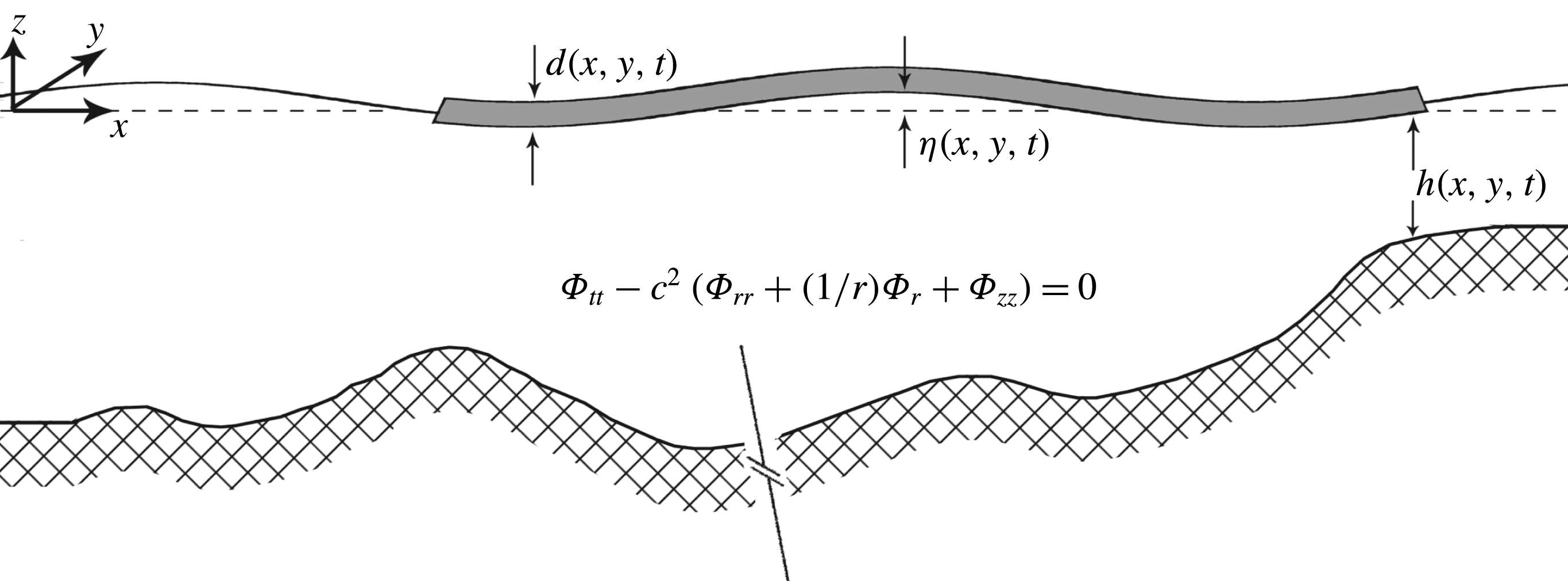
Schematic view of the fluid domain.
Due to the increasing effects of climate change and sea level rise, a rise in the frequency and destructiveness of natural disasters in arctic zones is foreseen (Hansen Reference Hansen2007). These include, but are not limited to, submarine earthquakes, and mass failure and oscillation of large ice blocks. The latter can be possibly triggered by storms, atmospheric and ocean currents, ice block shrinkage, ice slides and ice-quakes. To tackle this problem, a proper surface boundary condition is thus required. The vast majority of literature on the propagation of wave disturbances in a compressible ocean under the effects of gravity considers the upper boundary as a free surface, leading to the mutual generation of surface-gravity waves and AGWs. In the presence of a layer of ice on the surface, the properties of the aforementioned waves may change fundamentally. Recently, Kadri (Reference Kadri2016a ) studied the generation of AGWs by a vertically oscillating rigid ice block, and argued that at the given settings, and without elasticity, gravity waves cannot be accounted for, and acoustic modes propagate at very specific frequencies.
In the present paper, we examine the effects of elasticity, focusing on AGWs in a water column of depth
 $h(x,y,t)$
bounded by a rigid bottom, and allowing either a free surface or an elastic ice sheet at the surface of thickness
 $d(x,y,t)$
. The vertical coordinate,
 $z$
, is measured positively upwards from the undisturbed surface, and
 $x$
and
 $y$
denote the horizontal Cartesian coordinates, as illustrated in figure 1. The presence of an ice layer often requires deriving proper orthogonality relations (Zakharov Reference Zakharov2008). Nevertheless, note that here the acoustic–gravity length scale far exceeds the width of the ice layer, which is confined to the surface, and thus all energy initially found in the AGWs will effectively remain in the liquid layer. Therefore, transmission to or reflection from the ice layer is neglected. The governing equations are described in a velocity potential form and applied to a circular disturbance (§ 2). The role of an elastic ice sheet on the surface compared to a free surface and rigid ice sheet is investigated in § 3. An analytical closed form solution of the bottom pressure is derived, and computations are carried out for the case of constant depth (§ 4). Then, in order to emphasise the role of the ice sheets, we consider variable ice thickness, water depth and source, and a depth-integrated mild-slope equation is developed and validated (§§ 5 and 6). Finally, concluding remarks are given in § 7.
2 Governing equations
For a circular disturbance of radius
 $R$
, the governing equation in cylindrical form (
 $x^{2}+y^{2}=r^{2}$
) for linearised, inviscid motion in a compressible medium with velocity determined by the gradient of a potential,
 $\boldsymbol{u}=\unicode[STIX]{x1D735}\unicode[STIX]{x1D6F7}$
, is given by
 $$\begin{eqnarray}\unicode[STIX]{x1D6F7}_{tt}-c^{2}\left(\unicode[STIX]{x1D6F7}_{rr}+\frac{1}{r}\unicode[STIX]{x1D6F7}_{r}+\unicode[STIX]{x1D6F7}_{zz}\right)=0,\quad -h\leqslant z\leqslant 0,\end{eqnarray}$$
where
 $c$
is the sound speed in water. The bottom boundary condition is given by
 $$\begin{eqnarray}\displaystyle & \displaystyle \unicode[STIX]{x1D6F7}_{z}+h_{t}+\unicode[STIX]{x1D6F7}_{r}h_{r}=0,\hspace{14.45377pt}z=-h, & \displaystyle\end{eqnarray}$$
 $$\begin{eqnarray}\displaystyle & \displaystyle h_{t}=-\frac{\unicode[STIX]{x1D701}_{0}}{\unicode[STIX]{x1D70F}}{\mathcal{H}}\left(R^{2}-r^{2}\right){\mathcal{H}}(t(\unicode[STIX]{x1D70F}-t)), & \displaystyle\end{eqnarray}$$
where
 ${\mathcal{H}}$
is the Heaviside step function,
 $\unicode[STIX]{x1D701}_{0}$
is its final vertical displacement, and
 $\unicode[STIX]{x1D70F}$
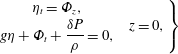
is the duration of its displacement. The kinematic and dynamic boundary conditions at the free surface, with an overlying ice sheet layer, are
 $$\begin{eqnarray}\left.\begin{array}{@{}c@{}}\unicode[STIX]{x1D702}_{t}=\unicode[STIX]{x1D6F7}_{z},\\ g\unicode[STIX]{x1D702}+\unicode[STIX]{x1D6F7}_{t}+\displaystyle \frac{\unicode[STIX]{x1D6FF}P}{\unicode[STIX]{x1D70C}}=0,\end{array}\quad z=0,\right\}\end{eqnarray}$$
where
 $g$
is the gravitational acceleration,
 $\unicode[STIX]{x1D70C}$
is the density of water and
 $\unicode[STIX]{x1D6FF}P$
is the pressure exerted by the moving ice sheet on the water column. Note that (2.1) neglects the background compressibility of the static water column. This effect is important for the long-range propagation of tsunamis, for example, but has been shown to be negligible for the acoustic modes of propagation; see Abdolali & Kirby (Reference Abdolali and Kirby2017). The equation for pressure exerted by an elastic ice sheet on the underlying water column is given by Schulkes, Hosking & Sneyd (Reference Schulkes, Hosking and Sneyd1987),
 $$\begin{eqnarray}\displaystyle \unicode[STIX]{x1D6FF}P=\unicode[STIX]{x1D70C}_{i}\,\text{d}\unicode[STIX]{x1D702}_{tt}+D\unicode[STIX]{x1D6FB}_{r}^{4}\unicode[STIX]{x1D702}+T\unicode[STIX]{x1D6FB}_{r}^{2}\unicode[STIX]{x1D702}, & & \displaystyle\end{eqnarray}$$
which includes the effect of the weight of the ice layer relative to its vertical motion, the effect of bending stress, and the effect of in-plane tension or compression in the ice layer (
 $T>0$
corresponds to compression). Note that the lateral stress
 $T$
has to be effectively large to impact wave propagation, therefore
 $T=0$
is taken in this study. Here we consider an ice sheet of density
 $\unicode[STIX]{x1D70C}_{i}=917~\text{kg}~\text{m}^{-3}$
, thickness
 $d$
, Young’s elastic modulus
 $E=10^{9}~\text{N}~\text{m}^{-2}$
and Poisson’s ratio
 $\unicode[STIX]{x1D708}=1/3$
. The flexural rigidity of ice is defined by Hosking, Sneyd & Waugh (Reference Hosking, Sneyd and Waugh1988),
 $$\begin{eqnarray}\displaystyle D=\frac{d^{3}E}{12(1-\unicode[STIX]{x1D708}^{2})}=c_{i}^{2}\unicode[STIX]{x1D70C}_{i}\frac{d^{3}}{12}, & & \displaystyle\end{eqnarray}$$
where
 $c_{i}=3700~\text{m}~\text{s}^{-1}$
is the sound speed in the ice layer. Combining the dynamic and kinematic boundary conditions at the surface equations (2.4) and (2.5) yields
 $$\begin{eqnarray}\unicode[STIX]{x1D70C}g\unicode[STIX]{x1D6F7}_{z}+\unicode[STIX]{x1D70C}\unicode[STIX]{x1D6F7}_{tt}+\unicode[STIX]{x1D70C}_{i}\,d\unicode[STIX]{x1D6F7}_{ttz}+D\unicode[STIX]{x1D6FB}_{r}^{2}(\unicode[STIX]{x1D6FB}_{r}^{2}\unicode[STIX]{x1D6F7}_{z})+T\unicode[STIX]{x1D6FB}_{r}^{2}\unicode[STIX]{x1D6F7}_{z}=0,\quad z=0.\end{eqnarray}$$
3 The role of the ice sheet
A calculation was carried out for the case of constant depth for different flexible ice sheet thicknesses on the surface compared to a free surface (
 $d=0$
). The governing equation in fluid and boundary conditions at the surface and bottom are defined in (2.1), (2.2), and (2.4). We used
 $h=1500~\text{m}$
,
 $\unicode[STIX]{x1D70C}=1024~\text{kg}~\text{m}^{-3}$
,
 $\unicode[STIX]{x1D70C}_{i}=917~\text{kg}~\text{m}^{-3}$
,
 $c=1500~\text{m}~\text{s}^{-1}$
,
 $c_{i}=3700~\text{m}~\text{s}^{-1}$
, for a unit source area with semilength
 $b=15$
km and
 $h_{t}=\sin (2\unicode[STIX]{x03C0}f_{0}t)$
for a rise time
 $\unicode[STIX]{x1D70F}=2/f_{0}=5$
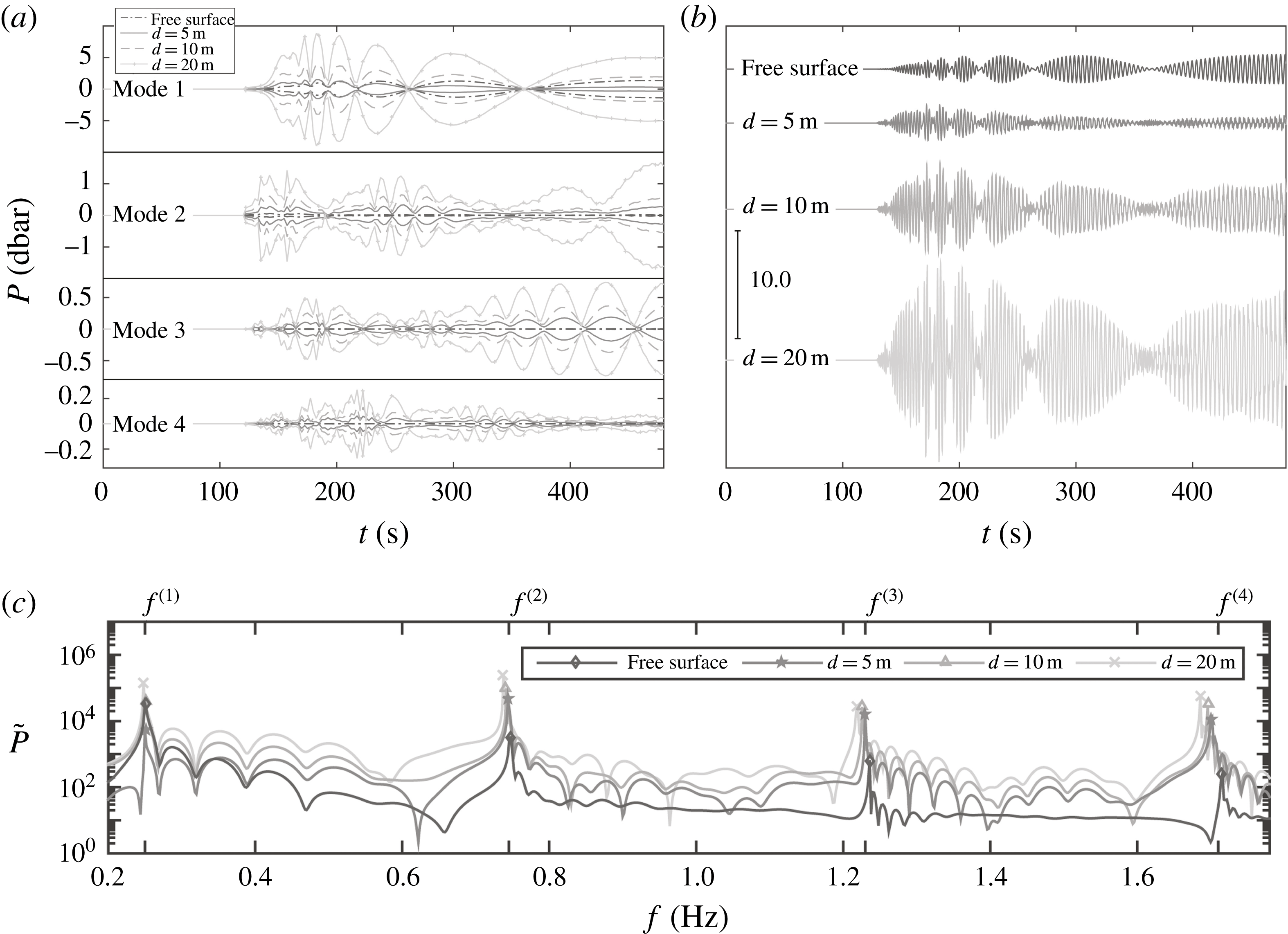
s. The results are depicted in figure 2 for the case of ice sheet thickness
 $d=0$
(black) and
 $d~=~5,~10$
and 20 m at 200 km from the epicentre. Panel (a) shows the envelope of pressure time series for the first four modes; panel (b) shows the superposition of acoustic modes
 $P$
; and panel (c) shows the corresponding frequency spectrum
 $\tilde{P}$
. For the free-surface boundary condition case (
 $d=0$
), the majority of energy is in the first mode. Increasing the ice thickness amplifies the pressure below the surface and also manifests in higher modes (unlike the case of the free surface).
The pressure time series and corresponding spectrum plotted 200 km from the epicentre at
 $z=0$
with varying ice thickness,
 $d=0$
(free surface), 5, 10 and 20 m, in a constant depth
 $h=1500$
m, for a unit source area with semilength
 $b=15$
km and
 $h_{t}=\sin (2\unicode[STIX]{x03C0}f_{0}t)$
for a rise time
 $\unicode[STIX]{x1D70F}=2/f_{0}=5$
s. (a) Envelope for the first four modes for different ice thicknesses. The comparison in each subplot is for each ice thickness comparing the amplitude of corresponding modes. (b) Superposition of the acoustic modes. (c) Frequency spectrum for the whole time series.
Pressure spectrum at
 $z=0$
for the cases of a free surface, and a rigid and flexible ice sheet (
 $d=30$
m), in a constant depth
 $h=3000$
m, for a unit source area with semilength
 $b=30$
km and
 $h_{t}=\sin (2\unicode[STIX]{x03C0}f_{0}t)$
for
 $f_{0}=0.55$
Hz, shown by the vertical dotted line, and a rise time
 $\unicode[STIX]{x1D70F}=2/f_{0}$
. The peak frequencies for the case of a rigid ice sheet on the surface can be evaluated using
 $f^{(n)}=nc/2h=0.25,0.5,0.75,1,\ldots$
Hz, while the cases of a free surface and flexible ice sheet can be approximated using
 $f^{(n)}=(2n-1)c/4h=0.125,0.375,0.625,0.825,\ldots$
Hz.

The frequency spectra of pressure signals at
 $z=0$
calculated from sets of computations, for the cases of a free surface, and rigid and flexible ice sheets on the surface are shown in figure 3. The water depth is
 $h=3000$
m, the semifault length
 $b=30$
km and
 $h_{t}=\sin (2\unicode[STIX]{x03C0}f_{0}t)$
for
 $f_{0}=0.55$
Hz. For the case of a rigid bottom, the peak frequencies are calculated using
 $f^{(n)}=nc/2h$
, whereas for the cases of a free surface and a flexible ice sheet, it can be evaluated using
 $f^{(n)}=(2n-1)c/4h$
, where
 $\unicode[STIX]{x1D714}=2\unicode[STIX]{x03C0}f$
.
4 Analytical solution
4.1 Dispersion relation
Defining the Fourier transform of the velocity potential
 $$\begin{eqnarray}\unicode[STIX]{x1D711}(r,z,\unicode[STIX]{x1D714})=\frac{1}{\sqrt{2\unicode[STIX]{x03C0}}}\int _{-\infty }^{\infty }\unicode[STIX]{x1D6F7}(r,z,t)\exp (-\text{i}\unicode[STIX]{x1D714}t)\,\text{d}t,\end{eqnarray}$$
the governing equation and boundary conditions become
 $$\begin{eqnarray}\displaystyle & \displaystyle \frac{\unicode[STIX]{x1D714}^{2}}{c^{2}}\unicode[STIX]{x1D711}+\unicode[STIX]{x1D6FB}_{r}^{2}\unicode[STIX]{x1D711}+\unicode[STIX]{x1D711}_{zz}=0,\quad -h\leqslant z\leqslant 0, & \displaystyle\end{eqnarray}$$
 $$\begin{eqnarray}\displaystyle & \displaystyle -\unicode[STIX]{x1D714}^{2}\unicode[STIX]{x1D711}+(g-\tilde{\unicode[STIX]{x1D70C}}\,\text{d}\unicode[STIX]{x1D714}^{2})+\tilde{D}\unicode[STIX]{x1D6FB}_{r}^{2}\left(\unicode[STIX]{x1D6FB}_{r}^{2}\unicode[STIX]{x1D711}_{z}\right)+\tilde{T}\unicode[STIX]{x1D6FB}_{r}^{2}\unicode[STIX]{x1D711}_{z}=0,\quad z=0, & \displaystyle\end{eqnarray}$$
 $$\begin{eqnarray}\displaystyle & \displaystyle \unicode[STIX]{x1D711}_{z}+\frac{\text{i}\unicode[STIX]{x1D701}_{0}}{\unicode[STIX]{x1D70F}\sqrt{2\unicode[STIX]{x03C0}}}\frac{1-\text{e}^{-\text{i}\unicode[STIX]{x1D714}\unicode[STIX]{x1D70F}}}{\unicode[STIX]{x1D714}}{\mathcal{H}}(R^{2}-r^{2}),\quad z=-h, & \displaystyle\end{eqnarray}$$
where
 $\unicode[STIX]{x1D6FB}_{r}^{2}$
is the horizontal gradient,
 $\tilde{\unicode[STIX]{x1D70C}}=\unicode[STIX]{x1D70C}_{i}/\unicode[STIX]{x1D70C}$
,
 $\tilde{D}=D/\unicode[STIX]{x1D70C}g$
,
 $\tilde{T}=T/\unicode[STIX]{x1D70C}g$
. Using the method of separation of variables, the field equation results in two ordinary differential equations, which upon substitution in the boundary conditions result in the dispersion relation,
 $$\begin{eqnarray}\unicode[STIX]{x1D714}^{2}=-\frac{g\unicode[STIX]{x1D706}_{n}\tan (\unicode[STIX]{x1D706}_{n}h)}{1-\tilde{d}\unicode[STIX]{x1D706}_{n}\tan (\unicode[STIX]{x1D706}_{n}h)}\left(1+\tilde{D}k_{n}^{4}-\tilde{T}k_{n}^{2}\right),\end{eqnarray}$$
where
 $\tilde{d}=\tilde{\unicode[STIX]{x1D70C}}d$
, subscript
 $n$
denotes the mode number, and
 $$\begin{eqnarray}\unicode[STIX]{x1D706}_{n}^{2}=\frac{\unicode[STIX]{x1D714}^{2}}{c^{2}}-k_{n}^{2}.\end{eqnarray}$$
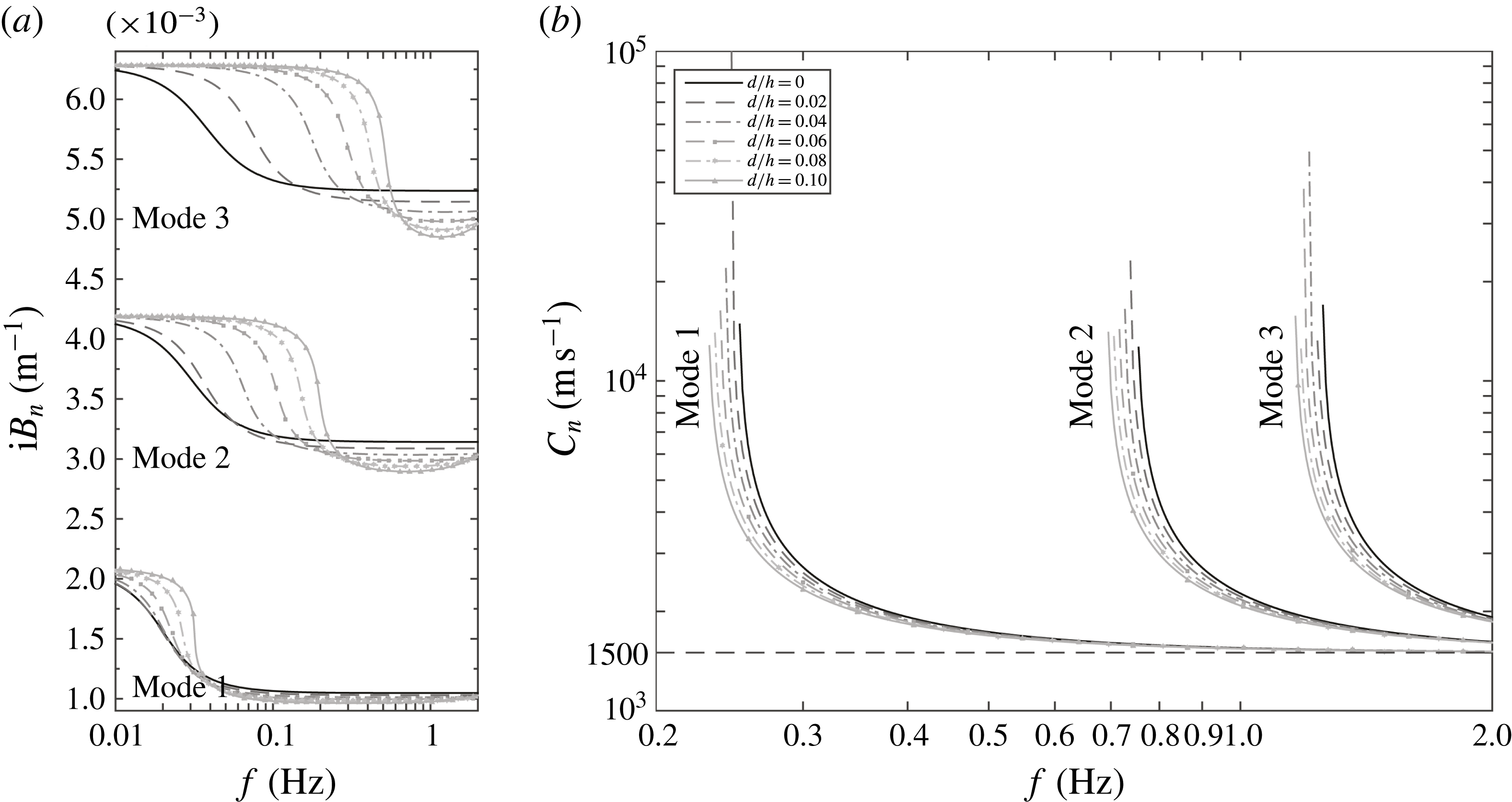
Gravity wavenumber
 $k_{r}^{2}=\unicode[STIX]{x1D714}^{2}/c^{2}+\unicode[STIX]{x1D706}_{0}^{2}$
for the imaginary roots of the dispersion relation
 $\unicode[STIX]{x1D706}_{0}$
(4.5) for varying ice sheet thickness
 $d/h$
(
 $a$
); corresponding phase celerity
 $c_{r}$
(
 $b$
). The solid black line is for the case of a free surface.

Dispersion relation solution for acoustic–gravity modes (
 $\unicode[STIX]{x1D706}_{n=1,2,3}$
) obtained from (4.5) for varying ice sheet thickness
 $d/h$
(
 $a$
); corresponding phase celerity (
 $b$
). The frequency range where
 $k_{n}^{2}=\unicode[STIX]{x1D714}^{2}/c^{2}+\unicode[STIX]{x1D706}_{n}^{2}\leqslant 0$
represents the evanescent mode where mode
 $n$
is not propagating. The solid black line is for the case of a free surface.
For AGWs,
 $\unicode[STIX]{x1D706}_{n}$
and
 $k_{n}$
are real, and
 $n=1,2,\ldots ,N$
, where
 $N$
is the highest possible AGW number; for the surface-gravity mode,
 $\unicode[STIX]{x1D706}_{0}$
is imaginary and
 $k_{0}$
is real; and for the evanescent modes,
 $k_{n}$
is imaginary, with
 $n>N$
. When there is no overlying ice sheet,
 $d=0$
, equation (4.5) reduces to the classical dispersion relation given by
 $\unicode[STIX]{x1D714}^{2}=-g\unicode[STIX]{x1D706}_{n}\tan (\unicode[STIX]{x1D706}_{n}h)$
. In figure 4, the gravity wavenumber
 $k_{r}$
and phase celerity
 $c_{r}=\unicode[STIX]{x1D714}/k_{r}$
are shown in panels (
 $a$
) and (
 $b$
), respectively, for varying ice sheet thickness
 $0\leqslant d/h\leqslant 0.1$
, where
 $h=1500$
m. Comparison between wavenumbers in the presence of an ice sheet and for the case of a free surface,
 $d=0$
, shows that, for lower frequencies, the gravity wavenumbers are identical, and at higher frequencies, the wavenumber is reduced with respect to the free-surface condition. It shows that inclusion of the elastic ice sheet in the dispersion relation is negligible for long-period waves such as tsunamis, tides and surges, while, for shorter waves, this effect is significant. On the other hand, in figure 5, the solutions of the dispersion relation for real separation variables
 $\unicode[STIX]{x1D706}_{n}$
are shown for the first three acoustic modes. For a given frequency, if
 $k_{n}^{2}=\unicode[STIX]{x1D714}^{2}/c^{2}-\unicode[STIX]{x1D706}_{n}^{2}\leqslant 0$
, the acoustic mode is evanescent, whereas for
 $k_{n}^{2}>0$
, the acoustic mode is progressive. In order to compare the separation variable changes due to the presence or absence of an ice sheet on the surface, values of
 $\unicode[STIX]{x1D706}_{n}$
are plotted for
 $0\leqslant d/h\leqslant 0.1$
in panel (
 $a$
). The corresponding phase celerity compared to the
 $d=0$
case is shown in panel (
 $b$
).
Rearranging (4.5) by isolating
 $\tan (\unicode[STIX]{x1D706}_{n}h)$
leads to the form
 $$\begin{eqnarray}\tan \left(\unicode[STIX]{x1D706}_{n}h\right)=\frac{1}{\unicode[STIX]{x1D706}_{n}\tilde{d}\left(1-\mathfrak{Ka}\right)\left(1+\tilde{D}k_{n}^{4}-\tilde{T}k_{n}^{2}\right)},\end{eqnarray}$$
where
 $\mathfrak{Ka}\equiv g/\tilde{d}\unicode[STIX]{x1D714}^{2}$
is a dimensionless quantity that accounts for the effects of gravity relative to oscillations in the ice sheet layer. This quantity can also be described by
 $\mathfrak{Ka}=Fr^{-1}St^{-2}$
, where
 $Fr$
and
 $St$
represent the Froude and Strouhal numbers. For the leading AGWs with corresponding
 $k_{n}\ll 1$
, the term
 $(\tilde{D}k_{n}^{4}-\tilde{T}k_{n}^{2})$
can be neglected, and the contribution of the ice sheet is encapsulated in the thickness of the ice sheet, or equivalently by
 $\mathfrak{Ka}$
. The eigenvalues change fundamentally depending on whether
 $\mathfrak{Ka}\gg 1$
or
 $\mathfrak{Ka}\ll 1$
, and can be approximated by
 $$\begin{eqnarray}\unicode[STIX]{x1D706}_{n}h=\left\{\begin{array}{@{}ll@{}}\displaystyle \left(n-{\textstyle \frac{1}{2}}\right)\unicode[STIX]{x03C0},\quad & \mathfrak{Ka}\gg 1,\\ \displaystyle (n-1)\unicode[STIX]{x03C0},\quad & \mathfrak{Ka}\ll 1.\end{array}\right.\end{eqnarray}$$
These unique characteristics for the propagation of AGWs under elastic ice sheets are illustrated in the graphical solution of (4.7) presented in figure 6. Note that for the physical AGW problem at hand, the prescribed frequency is
 $O(1)$
or more; for frequencies much smaller than unity the eigenvalues can be approximated by the rigid solution, though this scenario is not considered here as it is not physical.
Dispersion relation for
 $\unicode[STIX]{x1D714}=2\unicode[STIX]{x03C0}/10$
at depth
 $h=4000$
m with
 $\mathfrak{Ka}=25,~0.25$
and
 $0.025$
. The dash-dot lines and solid lines represent
 $\tan (\unicode[STIX]{x1D706}_{n}h)$
and the right-hand side (RHS) of (4.7), respectively. The solution of (4.7) at cross points are shown for each ice thickness. An asymmetric signature can be seen at higher modes when
 $\mathfrak{Ka}\ll 1$
.

Far-field bottom-pressure record for the first four AGW modes evaluated by analytical solution (4.19) at 1000 km from the epicentre for disturbance radius
 $R=15$
km, depth
 $h=4$
km, duration
 $\unicode[STIX]{x1D70F}=10$
s and vertical amplitude
 $\unicode[STIX]{x1D701}_{0}=1$
m. (a) Gravity wavenumber and the first four imaginary roots of the dispersion relation given by
 $k_{n}^{2}=\unicode[STIX]{x1D714}^{2}/c^{2}-\unicode[STIX]{x1D706}_{n}^{2}$
. Time series of the first four AGW modes (b) and the corresponding spectrum (c).
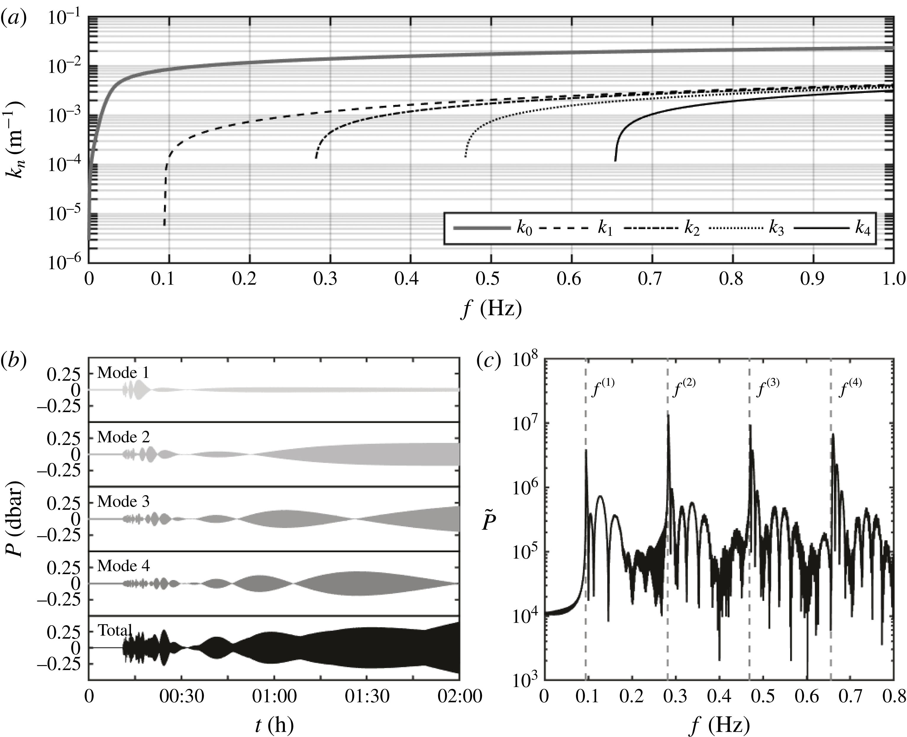
In figure 7(
 $a$
), gravity
 $k_{0}$
and the first four acoustic wavenumbers
 $k_{n}$
are shown for ice sheet thickness
 $d=20$
m with
 $h=4000$
m. For a given frequency, the wavenumber can be either evanescent if
 $k^{2}=\unicode[STIX]{x1D714}^{2}/c^{2}-\unicode[STIX]{x1D706}^{2}\leqslant 0$
or progressive if
 $k^{2}>0$
.
4.2 Far-field bottom pressure
The velocity potential is found by constructing inner
 $(r<R)$
and outer (
 $r>R$
) regions, following similar steps as presented by Hendin & Stiassnie (Reference Hendin and Stiassnie2013). For the inner region one needs to include a particular solution,
 $$\begin{eqnarray}s(z)=\frac{\text{i}\unicode[STIX]{x1D701}_{0}c}{\unicode[STIX]{x1D70F}\sqrt{2\unicode[STIX]{x03C0}}}\frac{1-\text{e}^{-\text{i}\unicode[STIX]{x1D714}\unicode[STIX]{x1D70F}}}{\unicode[STIX]{x1D714}^{2}}{\displaystyle \frac{\unicode[STIX]{x1D6FC}\cos \left({\displaystyle \frac{\unicode[STIX]{x1D714}}{c}}z\right)+\sin \left({\displaystyle \frac{\unicode[STIX]{x1D714}}{c}}z\right)}{\cos \left({\displaystyle \frac{\unicode[STIX]{x1D714}}{c}}h\right)+\unicode[STIX]{x1D6FC}\sin \left({\displaystyle \frac{\unicode[STIX]{x1D714}}{c}}h\right)}},\quad \unicode[STIX]{x1D6FC}={\displaystyle \frac{g-\tilde{d}\unicode[STIX]{x1D714}^{2}+\tilde{D}k^{4}}{\unicode[STIX]{x1D714}\,c}}.\end{eqnarray}$$
In the inner region the effect of the overlying ice sheet on the propagating modes is amplified. For a free surface,
 $\unicode[STIX]{x1D6FC}$
reduces to
 $g/\unicode[STIX]{x1D714}c$
and the solution originally obtained by Hendin & Stiassnie (Reference Hendin and Stiassnie2013) for a circular disturbance at the sea floor with a free-surface condition is retrieved. Following a standard matching technique between the inner and outer regions, and applying continuity at
 $r=R$
, we obtain a solution for the AGW modes in the outer region of the form
 $$\begin{eqnarray}\displaystyle & & \displaystyle \displaystyle \unicode[STIX]{x1D6F7}^{(out)}(r,z,t)=-\frac{4R\unicode[STIX]{x1D701}_{0}}{\unicode[STIX]{x1D70F}}\mathop{\sum }_{n=1}^{N}\int _{\unicode[STIX]{x1D714}_{sn}}^{\infty }\frac{\unicode[STIX]{x1D706}_{n}}{\unicode[STIX]{x1D714}k_{n}}\frac{\cos \unicode[STIX]{x1D706}_{n}(z+h)\sin (\unicode[STIX]{x1D714}\unicode[STIX]{x1D70F}/2)}{\sin (2\unicode[STIX]{x1D706}_{n}h)+2\unicode[STIX]{x1D706}_{n}h}\nonumber\\ \displaystyle & & \displaystyle \displaystyle \quad \times \,\text{J}_{1}(k_{n}R)\left[\text{J}_{0}(k_{n}r)\sin \left(\unicode[STIX]{x1D714}t-\frac{\unicode[STIX]{x1D714}\unicode[STIX]{x1D70F}}{2}\right)-\text{Y}_{0}(k_{n}r)\cos \left(\unicode[STIX]{x1D714}t-\frac{\unicode[STIX]{x1D714}\unicode[STIX]{x1D70F}}{2}\right)\right]\,\text{d}\unicode[STIX]{x1D714},\end{eqnarray}$$
where
 $\text{J}$
and
 $\text{Y}$
are Bessel functions of the first and second kinds. Finally, the bottom pressure is given by
 $p_{b}=-\unicode[STIX]{x1D70C}\unicode[STIX]{x1D6F7}_{t}$
; substituting into (4.10) yields the far-field bottom pressure
 $$\begin{eqnarray}\displaystyle p_{b}^{(out)} & = & \displaystyle \frac{4\unicode[STIX]{x1D70C}R\unicode[STIX]{x1D701}_{0}}{\unicode[STIX]{x1D70F}}\mathop{\sum }_{n=1}^{N}\int _{\unicode[STIX]{x1D714}_{sn}}^{\infty }\frac{\unicode[STIX]{x1D706}_{n}}{k_{n}}\frac{\sin \left(\unicode[STIX]{x1D714}\unicode[STIX]{x1D70F}/2\right)}{\sin (2\unicode[STIX]{x1D706}_{n}h)+2\unicode[STIX]{x1D706}_{n}h}\text{J}_{1}(k_{n}R)\nonumber\\ \displaystyle & & \displaystyle \times \,\left[\text{J}_{0}(k_{n}r)\cos \left(\unicode[STIX]{x1D714}t-\frac{\unicode[STIX]{x1D714}\unicode[STIX]{x1D70F}}{2}\right)+\text{Y}_{0}(k_{n}r)\sin \left(\unicode[STIX]{x1D714}t-\frac{\unicode[STIX]{x1D714}\unicode[STIX]{x1D70F}}{2}\right)\right]\,\text{d}\unicode[STIX]{x1D714}.\end{eqnarray}$$
In the far field, when
 $r$
is very large, the Bessel functions can be approximated asymptotically:
 $$\begin{eqnarray}\displaystyle \text{J}_{0}(k_{n}r)=\sqrt{\frac{2}{\unicode[STIX]{x03C0}k_{n}r}}\cos \left(k_{n}r-\frac{\unicode[STIX]{x03C0}}{4}\right), & & \displaystyle\end{eqnarray}$$
 $$\begin{eqnarray}\displaystyle \text{Y}_{0}(k_{n}r)=\sqrt{\frac{2}{\unicode[STIX]{x03C0}k_{n}r}}\sin \left(k_{n}r-\frac{\unicode[STIX]{x03C0}}{4}\right). & & \displaystyle\end{eqnarray}$$
Substituting the Bessel approximations back into the pressure relation gives
 $$\begin{eqnarray}\displaystyle p_{b}^{(out)} & = & \displaystyle \frac{4\unicode[STIX]{x1D70C}R\unicode[STIX]{x1D701}_{0}}{\unicode[STIX]{x1D70F}}\mathop{\sum }_{n=1}^{N}\int _{\unicode[STIX]{x1D714}_{sn}}^{\infty }\sqrt{\frac{2}{\unicode[STIX]{x03C0}k_{n}r}}\frac{\unicode[STIX]{x1D706}_{n}}{k_{n}}\frac{\sin \left(\unicode[STIX]{x1D714}\unicode[STIX]{x1D70F}/2\right)}{\sin (2\unicode[STIX]{x1D706}_{n}h)+2\unicode[STIX]{x1D706}_{n}h}\text{J}_{1}(k_{n}R)\nonumber\\ \displaystyle & & \displaystyle \times \,\cos \left(k_{n}r-\unicode[STIX]{x1D714}t+\frac{\unicode[STIX]{x1D714}\unicode[STIX]{x1D70F}}{2}-\frac{\unicode[STIX]{x03C0}}{4}\right)\,\text{d}\unicode[STIX]{x1D714}.\end{eqnarray}$$
Defining the phase of the
 $n$
-mode as
 $$\begin{eqnarray}g_{n}(\unicode[STIX]{x1D714})=k_{n}(\unicode[STIX]{x1D714})\frac{r}{t}-\unicode[STIX]{x1D714}\left(1-\frac{\unicode[STIX]{x1D70F}}{2t}\right)-\frac{\unicode[STIX]{x03C0}}{4t}\quad \text{where }k_{n}(\unicode[STIX]{x1D714})=\sqrt{\frac{\unicode[STIX]{x1D714}^{2}}{c^{2}}-\unicode[STIX]{x1D706}_{n}^{2}},\end{eqnarray}$$
the point of stationary phase is then at
 $\unicode[STIX]{x1D714}=\unicode[STIX]{x1D714}_{s,n}$
, where
 $\unicode[STIX]{x2202}g_{n}/\unicode[STIX]{x2202}\unicode[STIX]{x1D714}=0$
, so that
 $$\begin{eqnarray}\frac{\unicode[STIX]{x2202}g_{n}}{\unicode[STIX]{x2202}\unicode[STIX]{x1D714}}=\frac{\unicode[STIX]{x1D714}_{s,n}}{\sqrt{\unicode[STIX]{x1D714}_{s,n}^{2}/c^{2}-\unicode[STIX]{x1D706}_{n}^{2}}}\frac{r}{c^{2}t}-\left(1-\frac{\unicode[STIX]{x1D70F}}{2t}\right)=0,\end{eqnarray}$$
or by isolating
 $\unicode[STIX]{x1D714}_{s,n}$
,
 $$\begin{eqnarray}\unicode[STIX]{x1D714}_{s,n}=\frac{\unicode[STIX]{x1D706}_{s,n}c}{\sqrt{1-[r/c(t-\unicode[STIX]{x1D70F}/2)]^{2}}},\quad k_{s,n}=\frac{\unicode[STIX]{x1D706}_{s,n}}{\sqrt{[r/c(t-\unicode[STIX]{x1D70F}/2)]^{2}-1}},\end{eqnarray}$$
where
 $\unicode[STIX]{x1D706}_{s,n}$
obeys (4.8) and
 $$\begin{eqnarray}\frac{\unicode[STIX]{x2202}^{2}g_{n}}{\unicode[STIX]{x2202}^{2}\unicode[STIX]{x1D714}}=\frac{\unicode[STIX]{x1D706}_{s,n}^{2}r/c^{2}t}{\left(\unicode[STIX]{x1D714}_{s,n}^{2}/c^{2}-\unicode[STIX]{x1D706}_{s,n}^{2}\right)^{3/2}}.\end{eqnarray}$$
So finally we can write
 $$\begin{eqnarray}p_{b}=\frac{8\unicode[STIX]{x1D70C}R\unicode[STIX]{x1D701}_{0}c}{r\unicode[STIX]{x1D70F}}\mathop{\sum }_{n=1}^{N}\frac{\unicode[STIX]{x1D706}_{s,n}}{k_{s,n}}\frac{\sin \left(\displaystyle \frac{\unicode[STIX]{x1D714}_{s,n}\unicode[STIX]{x1D70F}}{2}\right)}{2\unicode[STIX]{x1D706}_{s,n}h}\text{J}_{1}\left(k_{s,n}R\right)\cos \left[k_{s,n}r-\unicode[STIX]{x1D714}_{s,n}\left(t-\frac{\unicode[STIX]{x1D70F}}{2}\right)-\frac{\unicode[STIX]{x03C0}}{4}\right].\end{eqnarray}$$
When
 $\mathfrak{Ka}\gg 1$
then (4.19) reduces to the free-surface solution (see e.g. Hendin & Stiassnie Reference Hendin and Stiassnie2013), whereas when
 $\mathfrak{Ka}\ll 1$
the eigenvalues change fundamentally. The solution of (4.19) for a circular disturbance of
 $R=15$
km with duration
 $\unicode[STIX]{x1D70F}=10$
s, residual displacement
 $\unicode[STIX]{x1D701}_{0}=1$
m,
 $d=20$
m and
 $h=4$
km are shown in figure 7. The results are presented in terms of bottom-pressure time series for the first four AGW modes, at a distance of 1000 km from the epicentre in panel (
 $b$
) with the corresponding spectrum in panel (
 $c$
).
5 Mild-slope equation for an elastic ice sheet
Next we develop a mild-slope equation (MSE) based on the eigenfunction structure for the problem with constant layer depths
 $h$
. Similar to the ideas of MSE, presented in Kirby (Reference Kirby1992) for an incompressible fluid, the solution of a system of ice–water–bottom as a waveguide is sought by wave equations in the water layer that satisfy the boundary conditions imposed by a possibly moving rigid sea bottom (i.e. an earthquake) and the flexible ice plate. Employing the governing equation and boundary conditions described in § 2, we derive a mild-slope model following a similar approach as described by Sammarco et al. (Reference Sammarco, Cecioni, Bellotti and Abdolali2013) and Abdolali et al. (Reference Abdolali, Kirby and Bellotti2015). Using the separation,
 $\unicode[STIX]{x1D6F7}=f(z)\unicode[STIX]{x1D713}(x,y,t)$
, we write the governing equation (2.1), which yields
 $$\begin{eqnarray}\frac{1}{c^{2}}(f\unicode[STIX]{x1D713})_{tt}-\unicode[STIX]{x1D6FB}_{r}^{2}(f\unicode[STIX]{x1D713})-f_{zz}\unicode[STIX]{x1D713}=0.\end{eqnarray}$$
Upon multiplication by
 $f$
and integration over the depth, followed by using Leibniz’s rule and the boundary conditions at the free surface and the bottom, we neglect second-order terms in the substrate slope, staying within the classic mild-slope framework and obtain the MSE:
 $$\begin{eqnarray}\displaystyle \left[\left(\frac{I_{1}^{n}}{c^{2}}+\frac{1}{g}\right)\unicode[STIX]{x1D713}_{n,t}\right]_{,t}-\unicode[STIX]{x1D735}_{r}\boldsymbol{\cdot }(I_{1}^{n}\unicode[STIX]{x1D735}_{r}\unicode[STIX]{x1D713}_{n})+I_{2}^{n}\unicode[STIX]{x1D713}_{n}+\frac{1}{\unicode[STIX]{x1D70C}g}\frac{\unicode[STIX]{x2202}}{\unicode[STIX]{x2202}t}(\unicode[STIX]{x1D6FF}P)-\frac{h_{n,t}}{\cosh (\unicode[STIX]{x1D706}_{n}h)}=0. & & \displaystyle\end{eqnarray}$$
Substituting (2.5) in (5.2) yields
 $$\begin{eqnarray}\displaystyle & & \displaystyle \displaystyle \left[\left(\frac{I_{1}^{n}}{c^{2}}+\frac{1}{g}\right)\unicode[STIX]{x1D713}_{n,t}\right]_{,t}-\unicode[STIX]{x1D735}_{r}\boldsymbol{\cdot }(I_{1}^{n}\unicode[STIX]{x1D735}_{r}\unicode[STIX]{x1D713}_{n})+I_{2}^{n}\unicode[STIX]{x1D713}_{n}\nonumber\\ \displaystyle & & \displaystyle \displaystyle \quad +\,\unicode[STIX]{x1D6FB}_{r}^{2}(\tilde{D}\unicode[STIX]{x1D6FB}_{r}^{2}\unicode[STIX]{x1D702}_{t})+\unicode[STIX]{x1D735}_{r}(\tilde{T}\unicode[STIX]{x1D735}_{r}\unicode[STIX]{x1D702}_{t})+\frac{\tilde{d}}{g}\unicode[STIX]{x1D702}_{ttt}-\frac{h_{n,t}}{\cosh (\unicode[STIX]{x1D706}_{n}h)}=0.\end{eqnarray}$$
Using the kinematic boundary condition at surface,
 $\unicode[STIX]{x1D702}_{t}=f_{z}|_{0}\unicode[STIX]{x1D713}_{n}=\unicode[STIX]{x1D706}_{n}\tanh (\unicode[STIX]{x1D706}_{n}h)\unicode[STIX]{x1D713}_{n}$
, we obtain the final form of the hyperbolic MSE for weakly compressible fluid in the arctic zones,
 $$\begin{eqnarray}\displaystyle & & \displaystyle \displaystyle \left[\left(\frac{I_{1}^{n}}{c^{2}}+\frac{1+\tilde{d}\unicode[STIX]{x1D706}_{n}\tanh (\unicode[STIX]{x1D706}_{n}h)}{g}\right)\unicode[STIX]{x1D713}_{n,t}\right]_{,t}-\unicode[STIX]{x1D735}_{r}\boldsymbol{\cdot }(I_{1}^{n}\unicode[STIX]{x1D735}_{r}\unicode[STIX]{x1D713}_{n})+I_{2}^{n}\unicode[STIX]{x1D713}_{n}\nonumber\\ \displaystyle & & \displaystyle \displaystyle \quad +\,\unicode[STIX]{x1D6FB}_{r}^{2}\left[\tilde{D}\unicode[STIX]{x1D6FB}_{r}^{2}\left(\unicode[STIX]{x1D706}_{n}\tanh (\unicode[STIX]{x1D706}_{n}h)\unicode[STIX]{x1D713}_{n}\right)\right]+\unicode[STIX]{x1D735}_{r}\left[\tilde{T}\unicode[STIX]{x1D735}_{r}\left(\unicode[STIX]{x1D706}_{n}\tanh (\unicode[STIX]{x1D706}_{n}h)\unicode[STIX]{x1D713}_{n}\right)\right]=\frac{h_{n,t}}{\cosh (\unicode[STIX]{x1D706}_{n}h)}.\end{eqnarray}$$
We allow slow variations in the ice properties (
 $D(x)$
and
 $T(x)$
). The model coefficients are
 $$\begin{eqnarray}I_{1}^{n}=\int _{-h}^{0}f^{2}\,\text{d}z=\frac{\sinh (2\unicode[STIX]{x1D706}_{n}h)+2\unicode[STIX]{x1D706}_{n}h}{4\unicode[STIX]{x1D706}_{n}\cosh ^{2}(\unicode[STIX]{x1D706}_{n}h)},\quad I_{2}^{n}=\int _{-h}^{0}f_{z}^{2}\,\text{d}z=\unicode[STIX]{x1D706}_{n}\frac{\sinh (2\unicode[STIX]{x1D706}_{n}h)-2\unicode[STIX]{x1D706}_{n}h}{4\cosh ^{2}(\unicode[STIX]{x1D706}_{n}h)}.\end{eqnarray}$$
It should be noted that the depth-integrated models cannot consider sharp changes, either of the ice properties or of the bottom topography. This is due to mild-slope variation of the parameters and also due to the absence of higher-order terms. Moreover, depth-integrated models cannot take into account any vertical variability of parameters, such as sound speed profile, which affect high-frequency signals.
6 Model validation
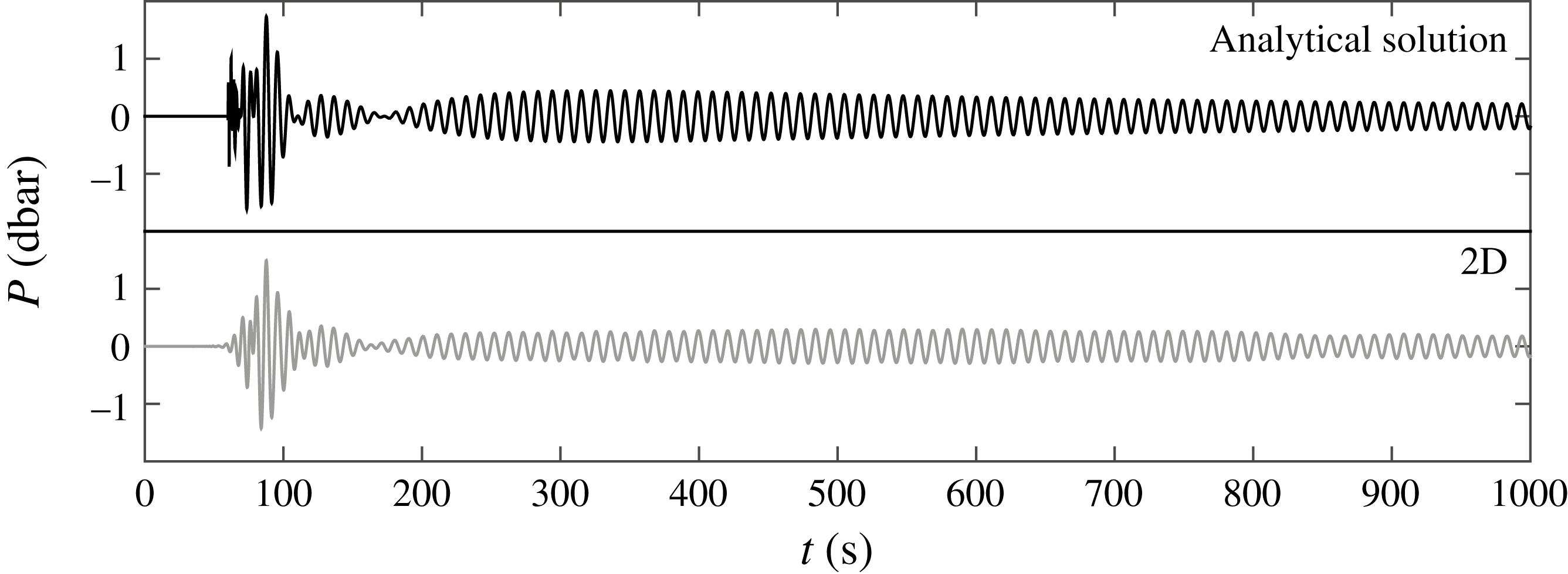
Sample computations have been carried out to verify if the 2D model in the form of a mild-slope approximation (5.4) along with the analytical solution (4.19) can replace the 3D model concerning the direct numerical solution of (2.1). Note that the 3D model refers to the numerical solution of (2.1) with boundary conditions defined by (2.2) and (2.4). To start with, the analytical solution is compared to the 2D model for the first AGW mode at a distance of
 $90$
km from the epicentre of a circular disturbance (
 $R=15$
) in a domain with 100 km radius. Although the analytical solution is based on an approximation for a relatively large distance (far field), we have chosen
 $90$
km from the epicentre to avoid lengthy numerical computations for the 2D model. For the 2D model, frequency bands of width
 $\unicode[STIX]{x0394}f=0.02$
Hz have been selected to discretise the forcing spectrum. The Sommerfeld radiation condition is applied at the outer open boundary, so that the waves leave the domain freely. To correctly reproduce the wavefield, for a given frequency the maximum mesh size is selected as
 $\unicode[STIX]{x0394}x=L/20$
, where
 $L$
is the wavelength. The time step is chosen according to the Courant number
 ${\leqslant}1$
. The summation of model output for narrow frequency bands (
 $0.05\leqslant f\leqslant 0.2$
) is in good agreement in terms of signal modulation, arrival time and peak frequency,
 $f^{(1)}=0.093$
Hz, with the analytical solution for the first acoustic mode (figure 8).
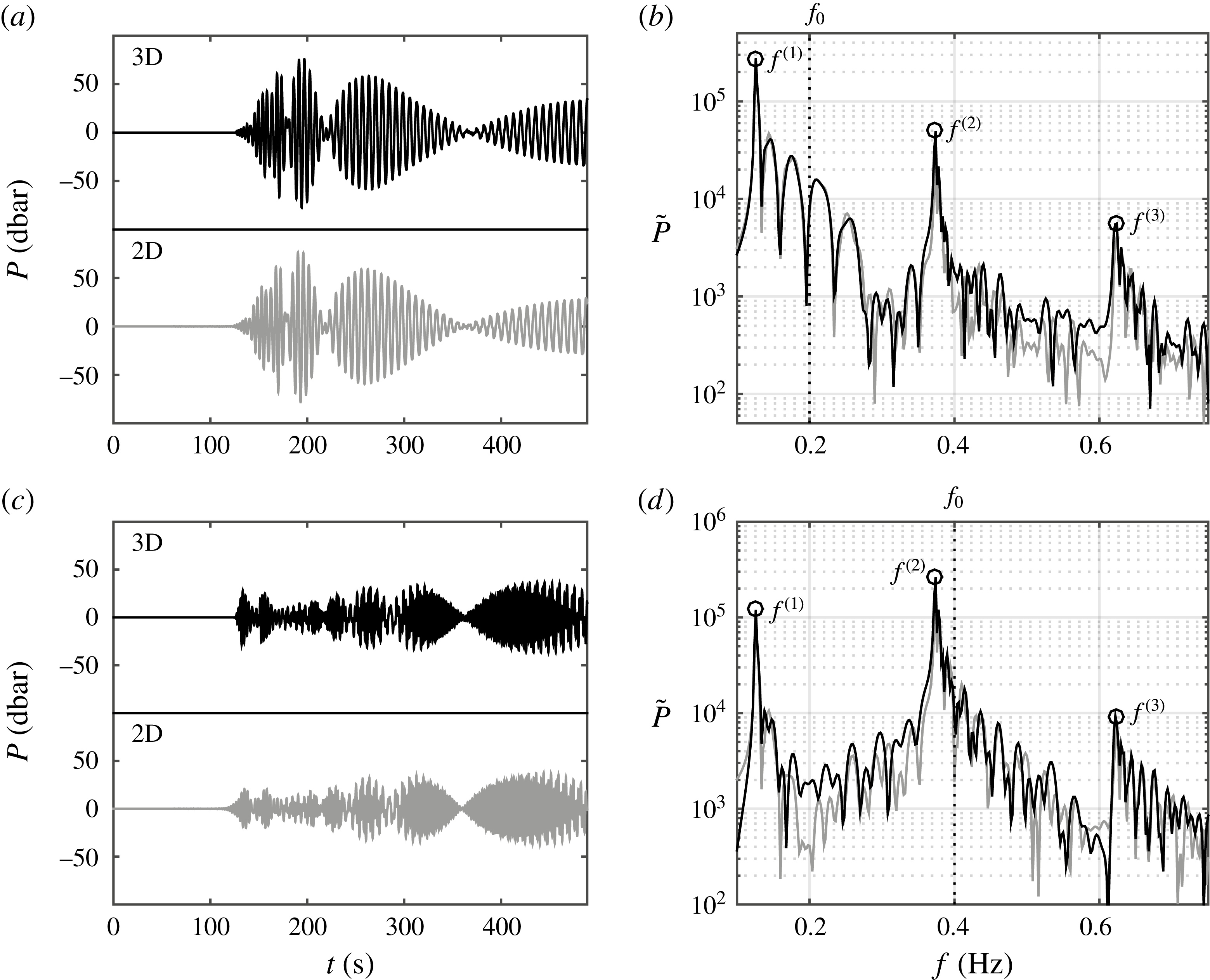
Bottom-pressure time series (a,c) and corresponding spectra (b,d) according to the 3D (black) and depth-integrated (light grey) models at
 $X=200$
km from the source and in a constant depth,
 $h=3000$
m,
 $d=20$
m; the water and ice characteristics are the same as in figure 7. For a unit source area with semilength
 $b=15$
km and
 $h_{t}=\sin (2\unicode[STIX]{x03C0}f_{0}t)$
with a rise time
 $\unicode[STIX]{x1D70F}=2/f_{0}$
. (a,b)
 $f_{0}=0.2$
Hz and
 $\unicode[STIX]{x1D70F}=10$
s and (c,d)
 $f_{0}=0.4$
Hz and
 $\unicode[STIX]{x1D70F}=5$
s.
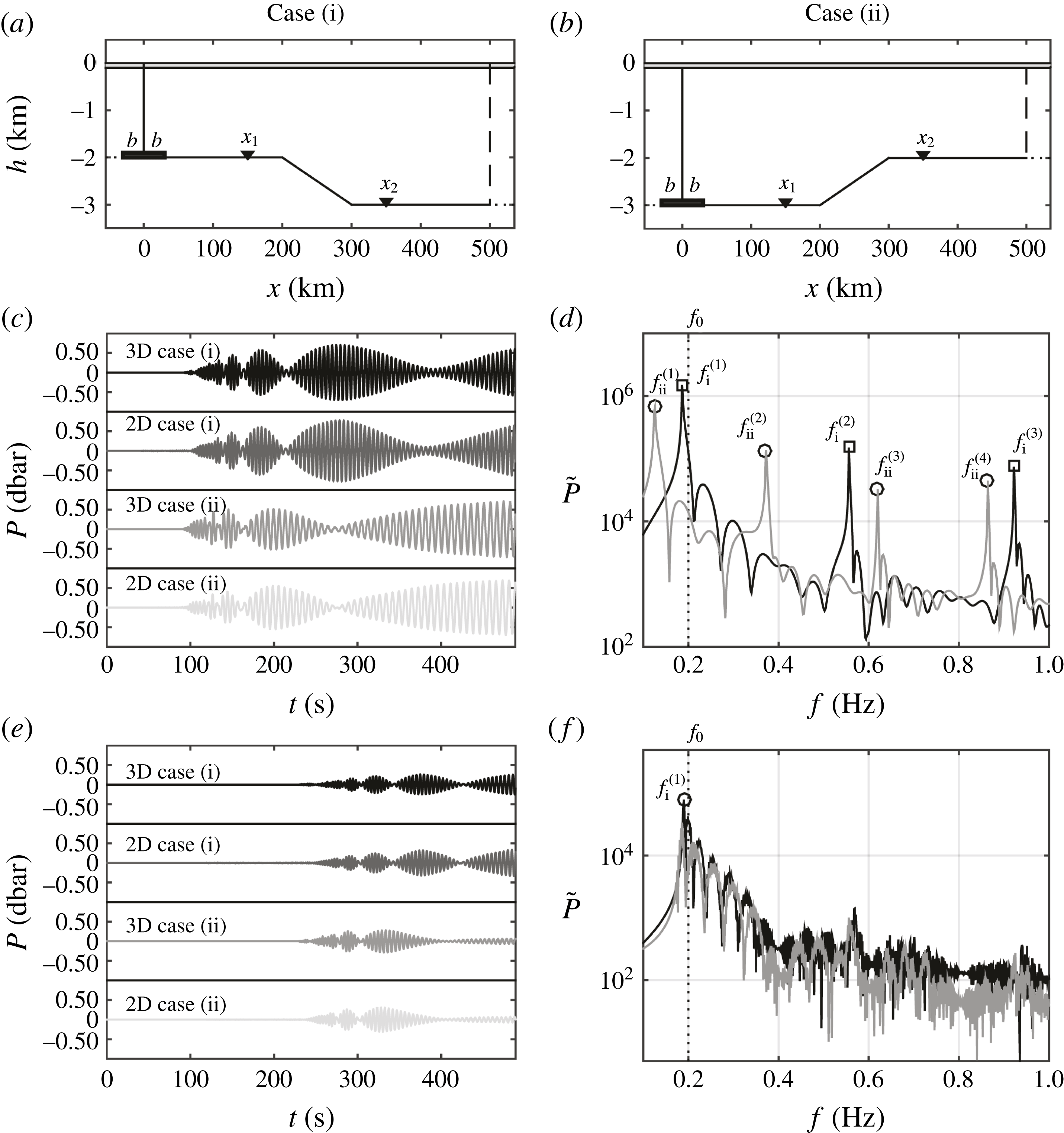
The case of varying sea bottom and constant ice sheet thickness with a tsunamigenic source at the shallower part (case i) and deeper part (case ii). (a,b) The computational domain. (c,e) Bottom-pressure time series and (d,f) corresponding spectra at point
 $X_{1}$
, 150 km, and point
 $X_{2}$
, 350 km from the source, respectively. For a unit source area with semilength
 $b=15$
km,
 $d=20$
m and
 $h_{t}=\sin (2\unicode[STIX]{x03C0}f_{0}t)$
with a rise time
 $\unicode[STIX]{x1D70F}=1/f_{0}=5$
s.
The case of varying sea bottom and partial ice sheet coverage over the surface with a tsunamigenic source at the shallower part. (a) The computational domain. (b,c) Bottom-pressure time series and corresponding spectrum at point
 $X_{1}$
, 100 km from the tsunamigenic source; (d,e) bottom-pressure time series and corresponding spectrum at point
 $X_{2}$
, 360 km from the tsunamigenic source. The water and ice sheet characteristics are the same as in figure 2. For a unit source area with semilength
 $b=15$
km,
 $d=15$
m and
 $h_{t}=\sin (2\unicode[STIX]{x03C0}f_{0}t)$
with a rise time
 $\unicode[STIX]{x1D70F}=1/f_{0}=5$
s.
In the second case, we validate the solutions for the case of constant depth
 $h=3$
km and ice coverage
 $d=20$
m. The domain consists of a vertical section in
 $x$
–
 $z$
through laterally uniform domains with no
 $y$
-dependency. The source fault has a semilength of
 $b=15$
km with a maximum vertical displacement of
 $\unicode[STIX]{x1D701}_{0}=1$
m. The numerical solvers are applied on a computational domain 500 km in length; given the symmetry of the problem about the middle of the earthquake (
 $x=0$
), a fully reflective boundary condition is applied and computations are undertaken only for half of the physical domain. The computational time needed to reproduce 500 s of real-time simulation was approximately an order of magnitude less than for the 3D model. The results are presented for a virtual bottom gauge at
 $x=200$
km in figure 9 in terms of the bottom pressure
 $P$
and the corresponding spectrum
 $\tilde{P}$
. Results in panels (a,b) relate to the case of
 $f_{0}=0.2$
Hz and
 $\unicode[STIX]{x1D70F}=10$
s, while those in panels (c,d) relate to the case of
 $f_{0}=0.4$
Hz and
 $\unicode[STIX]{x1D70F}=5$
s. The 3D model (black) and depth-integrated model (light grey) are in optimal agreement. The first three peak frequencies correspond to the cutoff frequency. The maximum number of AGW modes,
 $N_{max}$
, is determined from (4.6) and (4.8), with
 $k_{n}=0$
(corresponding to the cutoff frequency), so that
 $$\begin{eqnarray}N_{max}=\left\{\begin{array}{@{}ll@{}}\left\lfloor \unicode[STIX]{x1D714}h/c\unicode[STIX]{x03C0}+\frac{1}{2}\right\rfloor , & \mathfrak{Ka}\gg 1,\\ \left\lfloor \unicode[STIX]{x1D714}h/c\unicode[STIX]{x03C0}+1\right\rfloor , & \mathfrak{Ka}\ll 1,\end{array}\right.\end{eqnarray}$$
where the special brackets represent the floor function, i.e. largest integer from below. In the case
 $\mathfrak{Ka}\ll 1$
all progressive acoustic modes have to be considered in order to capture the whole spectrum properly, in particular upon transmission to shallower waters.
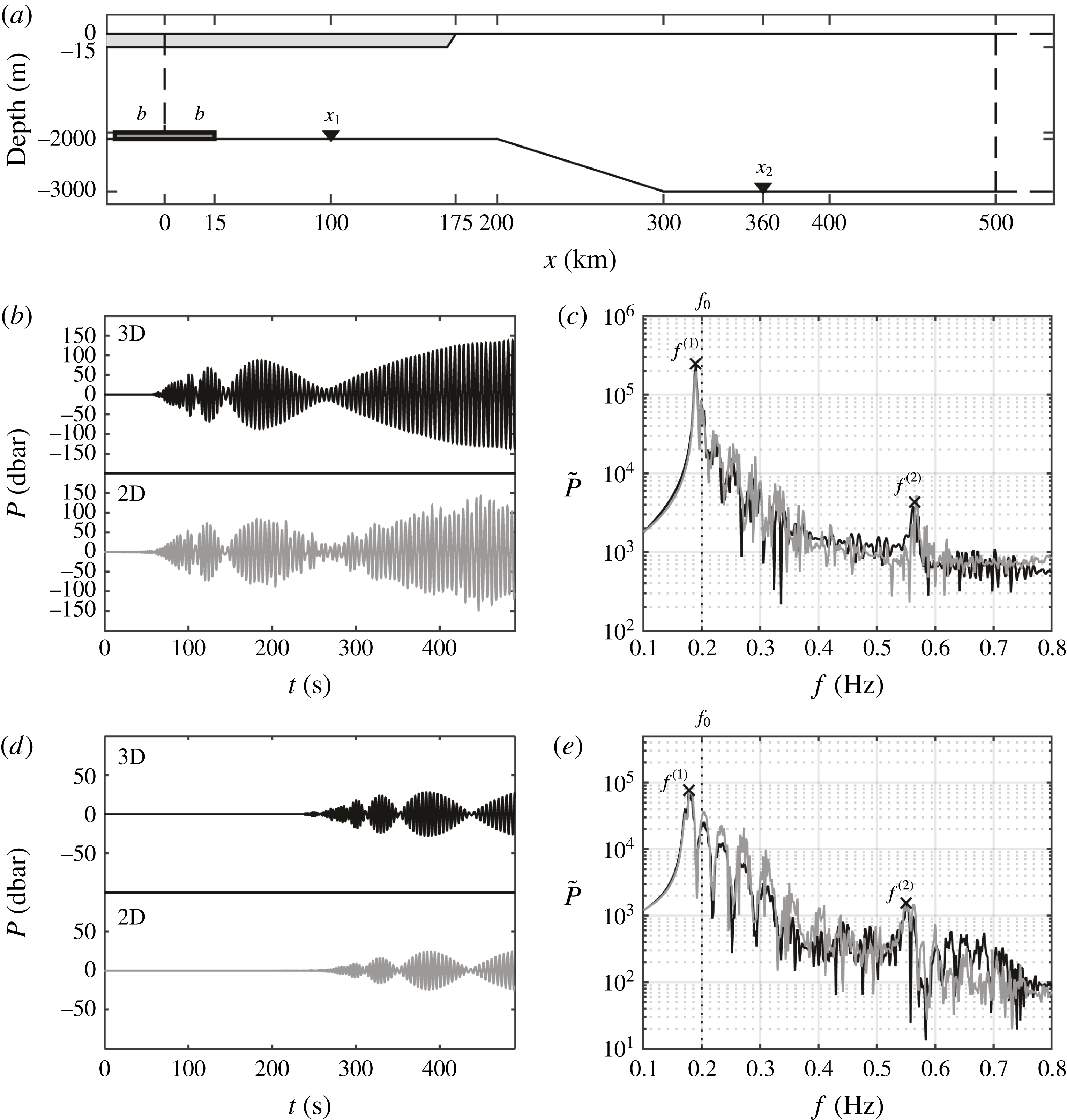
In the third case, a varying sea water depth with constant ice sheet thickness is considered in order to reveal AGW properties in deep and shallow water for the case of an earthquake in the shallower part of the continental shelf (case i) and in the deeper part of the computational domain (case ii). In figure 10, panels (a,b) depict the domain geometries, while panels (c,d) and (e,f) present the results in terms of bottom pressure at distances of
 $X_{1}=150$
and
 $X_{2}=350$
km, respectively, from the moving sea bed. For case i, where the water depth at the generation zone is 2 km, the first three peak frequencies are approximately
 $0.187$
,
 $0.56$
and
 $0.93$
Hz, which can propagate towards points
 $X_{1}$
and
 $X_{2}$
, as there is enough room in the wave guide. On the other hand, for case ii, the shallower part on the right-hand side of the domain filters out the first acoustic mode at the source depth and, therefore, only the signals at frequencies higher than
 $0.187$
Hz can reach point
 $X_{2}$
. The results from the 3D and 2D solvers are in good agreement in terms of amplitude, modulation and peak frequencies.
In the fourth case, the domain is partially covered by a 175 km long ice sheet with
 $d=15$
m thickness (figure 11). The rest of the numerical domain is subjected to barometric pressure (
 $d=0$
). The bed deformation, ice and water characteristics have the same values as previously. The bottom-pressure time series are plotted at
 $X_{1}=100$
km in 2 km depth with an ice sheet on the surface in panels (b,c) and at
 $X_{2}=360$
km in 3 km depth with a free-surface boundary in panels (d,e). As is shown in figure 11, the formation of acoustic–gravity waves in the source region is characterised by the local depth and ice sheet properties, where both 3D (black) and 2D (light grey) models have similar time series and frequency spectra.
7 Concluding remarks
We studied the effects of ice sheets on propagating acoustic–gravity waves (AGWs) in both constant and varying water depths. To this end, we present an analytical model along with numerical 2D depth-integrated and 3D models. The analytical model is only valid for constant depths, though it is computationally fast and accurate and can be employed for sensitivity analysis, as well as to estimate the source geometry. For large domains, the 3D model becomes computationally demanding, and thus a validation of the 2D model against the analytical solution was carried out. Note that the 2D model is in addition validated against the 3D model on a transect which resembles an infinite fault. The 2D model enables relatively fast calculations for real ocean floor geometries with partial ice coverage. It turns out that the dynamics of bed deformation affect the leading mode, which is determined by
 $N_{max}$
given by (6.1).
This work extends the capabilities of previous compressible models (Hendin & Stiassnie Reference Hendin and Stiassnie2013; Sammarco et al. Reference Sammarco, Cecioni, Bellotti and Abdolali2013; Abdolali et al. Reference Abdolali, Kirby and Bellotti2015) to include the effect of an elastic ice sheet on the sea surface, following the ideas in Kirby (Reference Kirby1992). Indeed, by expanding the capabilities of the model equation, the AGW field can be investigated in an integrated system of either bounded or free-surface oceans.
Acknowledgement
A.A. and J.T.K. acknowledge the support of the NSF Engineering for Natural Hazards program, grant CMMI-1537232.



