1 Introduction
We may say that plasma-based accelerators (Tajima & Dawson Reference Tajima and Dawson1979; Katsouleas & Dawson Reference Katsouleas and Dawson1983; Joshi & Katsouleas Reference Joshi and Katsouleas2003) and cosmic-ray acceleration (Fermi Reference Fermi1949; Carlson Reference Carlson2012; Ohsawa Reference Ohsawa2014) are both major unsolved problems in plasma physics. Rather than offer a global perspective on them, this paper focuses on specific plasma phenomena that have been found in the studies related to the two subjects.
In plasma-based accelerators, dephasing, i.e. energized electrons’ outrunning the accelerating phase of the wave, is one of the major factors limiting energy gain. In 2012, Schmit and Fisch proposed a new method to overcome this effect by modulating the phase velocity of an accelerating plasma wave by using an externally generated time-varying, uniform axial magnetic field (Schmit & Fisch Reference Schmit and Fisch2012). Gueroult and Fisch (referred to as GF below) then studied, with one-dimensional particle-in-cell (PIC) simulations, the practicality of magnetic compression for plasma density control (Gueroult & Fisch Reference Gueroult and Fisch2016). Generating two counter-propagating shock waves, they investigated compression of the plasma. Their simulations show that these shock waves reflect some ions and that these reflected ions lead to a non-uniform plasma density profile. In addition to the contributions to the research of plasma-based accelerators, as is shown below, their simulations have important implications for basic plasma physics and astrophysics.
Yamauchi and Ohsawa (referred to as YO below) explored in 2007 how shock waves are created from explosions in collisionless plasmas, such as solar flares and supernova explosions (Yamauchi & Ohsawa Reference Yamauchi and Ohsawa2007, Reference Yamauchi and Ohsawa2008). With one-dimensional PIC simulations, they studied the collision of exploding and surrounding plasmas; initially, the exploding plasma has a high velocity
 $v$
perpendicular to a magnetic field toward the surrounding plasma at rest. It is found that forward and backward shock waves form around the time
 $\unicode[STIX]{x1D6FA}_{i0}t\sim 1$
after the collision of the two plasmas, where
 $\unicode[STIX]{x1D6FA}_{i0}$
is the ion gyrofrequency for the external magnetic field, away from the initial boundary of the two plasmas by
 ${\sim}v/\unicode[STIX]{x1D6FA}_{i0}$
.
The beams of reflected ions in GF’s simulations have lower speeds and densities than those of the exploding ions in YO’s simulations. The maximum beam speed in GF’s simulations is
 $v\sim 5v_{A}\sim 0.02c$
, where
 $v_{A}$
is the Alfvén speed and
 $c$
is the speed of light, and the beam density is lower than that of the background plasma. The initial speed of the exploding ions in YO’s simulations is taken to be of the order of
 $c$
, and their density is greater than that of the surrounding plasma. (When looking at these values, we must note that the basic parameters of the two simulations are not the same; for instance, the ion-to-electron mass ratio is
 $m_{i}/m_{e}=1846$
in GF’s simulations, while it is
 $m_{i}/m_{e}=100$
in YO’s simulations.) Since YO’s ion speed is high, the ion gyroradius is large unless the magnetic field is too strong; for this reason, the system size of the simulations must be large. In fact, shock formation processes in the interstellar medium are large-scale phenomena (Spitzer Reference Spitzer1978, p. 255): a proton with a speed
 $v=10^{9}~\text{cm}~\text{s}^{-1}$
in a magnetic field
 $B=10^{-6}$
G has a gyroradius
 $\unicode[STIX]{x1D70C}_{i}~(=v/\unicode[STIX]{x1D6FA}_{i0})=1.0\times 10^{11}$
cm.
Interestingly, despite these differences, we find surprising similarities between the phenomena arising from the reflected ions (Gueroult & Fisch Reference Gueroult and Fisch2016) and those from the exploding ions (Yamauchi & Ohsawa Reference Yamauchi and Ohsawa2007).
The exploding ions penetrating into the surrounding plasma across a magnetic field in YO’s simulations can be viewed as unmagnetized in the early phase (
 $\unicode[STIX]{x1D6FA}_{i0}t\ll 1$
), while all the electrons are always magnetized. Because of the magnetic force, however, those exploding ions are significantly deflected around the time
 $\unicode[STIX]{x1D6FA}_{i0}t\sim 1$
, when the plasma density and the magnetic-field strength increase near the front of the exploding ions; a bump of magnetic field and plasma density forms.
If we replace the phrase ‘exploding ions’ by ‘reflected ions’ and ‘surrounding plasma’ by ‘background plasma’, the description in the above paragraph is also applicable to the phenomena in GF’s simulations.
After the creation of the bump, however, its evolution and effects on the plasma in GF’s simulations show some differences from those in YO’s simulations. The differences arise because the beam of YO’s exploding ions is much more intense (faster and denser) than the beam of GF’s reflected ions.
In this paper, we examine the similarities and differences of the plasma phenomena in the two papers. Although the main concern of the GF’s paper is plasma-based accelerators, we discuss the phenomena from the aspects of beam dynamics in a magnetized plasma, nonlinear wave evolution and pulse formation processes. In § 2, we compare some of the results of GF’s and YO’s simulations. In both simulations, a bump appears at
 $\unicode[STIX]{x1D6FA}_{i0}t\sim 1$
near the front part of the ion beam and affects the motion of neighbouring particles. The pulse created by YO’s exploding ions grows larger and reflects exploding ions backward and surrounding ions forward. Through these processes, YO’s pulse evolves into two magnetosonic pulses; one propagating backward in the exploding plasma and the other propagating forward in the surrounding plasma. Section 3 gives a summary of our analysis and a discussion on the effect of basic simulation parameters.
2 Comparison of two simulations
2.1 Reflected ions and foot
Ion reflection by a shock wave in a magnetic field has been studied by many authors (Morawetz Reference Morawetz1961; Biskamp & Welter Reference Biskamp and Welter1972; Forslund, Quest, Brackbill & Lee Reference Forslund, Quest, Brackbill and Lee1984; Ohsawa Reference Ohsawa1985; Tokar, Gary & Quest Reference Tokar, Gary and Quest1987; Ohsawa Reference Ohsawa1990, Reference Ohsawa2014). In GF’s simulations, the size of the foot ahead of a shock wave is rather large,
 ${\sim}10$
per cent of the plasma width, so that we can precisely observe the motion of reflected ions and their effects on the background plasma.
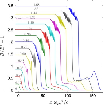
Spatial profile of magnetic field for different times. Growing and steepening are seen in the front part of the foot. Reproduction of figure 6(a) in Gueroult & Fisch (Reference Gueroult and Fisch2016).

In GF’s simulations, a one-dimensional (one space coordinate and three velocities), fully electromagnetic, relativistic PIC code is used to model plasma dynamics. Initially, the plasma slab is in the region
 $0<x<2\unicode[STIX]{x0394}x^{\circ }$
, where the superscript
 $\circ$
denotes the initial value. The plasma width is
 $2\unicode[STIX]{x0394}x^{\circ }=22$
mm, which is nearly
 $375c/\unicode[STIX]{x1D714}_{pe}^{\circ }$
, where
 $\unicode[STIX]{x1D714}_{pe}$
is the electron plasma frequency. The plasma is surrounded by a vacuum region with the width
 $3\unicode[STIX]{x0394}x^{\circ }/2$
on each side. These plasma and vacuum regions are immersed in a uniform external magnetic field that points in the
 $z$
direction. Magnetic compression ramps are generated at the left and right boundaries of the simulation domain and propagate toward the plasma region.
Figure 1, which is figure 6(a) in GF’s 2016 paper, shows spatial profiles of the magnetic field of a shock wave in the left half of the plasma domain. In the right half of the domain, which is not shown here, we have a left-going shock wave with its field profiles nearly symmetrical to those in the left domain. We find a foot in the magnetic-field profile upstream of the shock wave. This foot is formed owing to the reflection of the upstream ions by the shock wave. The plasma density also has a foot with a profile similar to that of the magnetic field (see figure 6b in GF’s paper).
The magnetic field and plasma density are growing in the front part of the foot around the time
 $\unicode[STIX]{x1D6FA}_{i0}t\sim 1$
; a bump is being created. It is stated in GF’s paper that the deflection of reflected ions by the magnetic field is responsible for the formation of the local field maximum upstream of the shock.
The author believes that this bump is evolving into a magnetosonic pulse. The fact that the magnetic field and plasma density have nearly the same profile and propagation speed suggests that collective effects are working in the bump. If this conjecture is correct, the following phenomena are expected:
-
(i) The bump has an electric potential
 $\unicode[STIX]{x1D719}$
with a profile nearly the same as the magnetic field and plasma density (if the influence of the beam on
$\unicode[STIX]{x1D719}$
is weak),
-
(ii) electron currents stronger than ion currents flow on both sides of the bump and
-
(iii) the magnetic, density and potential bumps all propagate with a speed slightly higher than the Alfvén speed, as magnetosonic solitary waves do (Adlam & Allen Reference Adlam and Allen1958; Gardner & Morikawa Reference Gardner and Morikawa1965).


The second point is a result of momentum conservation in perpendicular magnetosonic waves (see Ohsawa Reference Ohsawa2014, p. 156). The bump that is thought to be a magnetosonic pulse is called the (magnetosonic) pulse below.
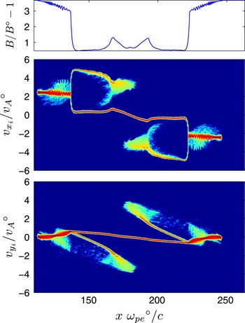
Figure 2, which is figure 7(a) in GF’s 2016 paper, gives a magnetic-field profile and ion phase space plots in the whole plasma region. Since the profile is nearly symmetric with respect to the central axis, we only look at the left half of the domain. The shapes of reflected and background ions in the phase space significantly change near the peak position of the pulse (
 $x\unicode[STIX]{x1D714}_{pe}^{\circ }/c\simeq 166$
), indicating that the pulse is affecting the ion motion considerably. We clearly see that the background ions are pushed forward (to the right) near the pulse. The pulse would be exerting a force in the negative
 $x$
direction on the reflected ions that have reached the pulse from the left side.
Ion phase space and magnetic-field profile prior to the interaction of the counter-propagating ion beams. The change in the structure of the phase space is noticeable near the two magnetic bumps. Reproduction of figure 7(a) in Gueroult & Fisch (Reference Gueroult and Fisch2016).

Ion reflection by a shock wave is not a rare phenomenon. Its study is therefore important. The number of ions reflected by a large-amplitude shock wave can be great even in a low beta plasma, where beta is the ratio of the plasma to magnetic pressures. The number is determined primarily by the ion thermal speed
 $v_{Ti}$
, the Alfvén speed
 $v_{A}$
and the Mach number
 $M$
. If
 $v_{Ti}$
is much lower than
 $v_{A}$
, then
 $f(Mv_{A})$
, the value of the ion velocity distribution function at the pulse speed
 $v_{ix}=Mv_{A}$
, would be quite small. However, nonlinear magnetosonic pulses can reflect ions with
 $v_{ix}$
greater than the velocity
 $$\begin{eqnarray}v_{ref}=Mv_{A}-(2e\unicode[STIX]{x1D719}/m_{i})^{1/2},\end{eqnarray}$$
where
 $\unicode[STIX]{x1D719}$
is the potential in the pulse (Ohsawa Reference Ohsawa2014, p. 241). The potential
 $\unicode[STIX]{x1D719}$
is approximately given by
 $$\begin{eqnarray}e\unicode[STIX]{x1D719}=2m_{i}v_{A}^{2}(M-1),\end{eqnarray}$$
for
 $1<M<2$
, indicating that
 $\unicode[STIX]{x1D719}$
can be quite large if the external magnetic field is strong and the Mach number is
 $M-1\sim O(1)$
. Thus,
 $v_{ref}$
can be much smaller than
 $Mv_{A}$
, and
 $f(v_{ref})$
can be comparable to
 $f(v_{Ti})$
; accordingly, a large number of ions can be reflected even in low beta plasmas. For shock waves with
 $M>2$
, the electric potential is given by
 $$\begin{eqnarray}e\unicode[STIX]{x1D719}=m_{i}v_{A}^{2}\left(\sin ^{2}\unicode[STIX]{x1D703}+\frac{\sin \unicode[STIX]{x1D703}\cos \unicode[STIX]{x1D703}}{\unicode[STIX]{x1D6FE}_{sh}(1+\unicode[STIX]{x1D6FE}_{sh}^{2}\tan ^{2}\unicode[STIX]{x1D703})^{1/2}}\right)\left[\left(1+\frac{2v_{sh}^{2}}{v_{A}^{2}\sin ^{2}\unicode[STIX]{x1D703}}\right)^{1/2}-1\right],\end{eqnarray}$$
where
 $\unicode[STIX]{x1D703}$
is the angle between the external magnetic field and the direction of the shock propagation (
 $\unicode[STIX]{x1D703}=90^{\circ }$
indicates perpendicular propagation),
 $v_{sh}$
is the shock speed and
 $\unicode[STIX]{x1D6FE}_{sh}$
is the Lorentz factor corresponding to
 $v_{sh}$
(Miyahara, Kawashima & Ohsawa Reference Miyahara, Kawashima and Ohsawa2003). If we substitute
 $e\unicode[STIX]{x1D719}$
given by (2.3) for
 $e\unicode[STIX]{x1D719}$
in (2.1) and replace
 $Mv_{A}$
with
 $v_{sh}$
, we obtain
 $v_{ref}$
for
 $M>2$
.
The sharp rise of the magnetic field in the front part of a shock wave also contributes to ion reflection (Kawashima, Miyahara & Ohsawa Reference Kawashima, Miyahara and Ohsawa2003). This effect is not taken into account in (2.1) because the magnetic field is assumed to be uniform in its derivation. For a more quantitative discussion on the fraction of reflected ions, we need to include the effect of the spatial variation of the magnetic field.
2.2 Collision of two plasmas and formation of forward and backward magnetosonic pulses
Now let us discuss the simulations of pulse formation from a collision of exploding and surrounding plasmas (Yamauchi & Ohsawa Reference Yamauchi and Ohsawa2007). Although the pulses discussed here were called shock waves in YO’s 2007 article, we here use the term ‘pulse’ to avoid confusion with the shock wave in GF’s 2016 paper: the bump in their paper corresponds to the pulse (or shock wave) in YO’s paper. A one-dimensional PIC code is also used here: at
 $t=0$
, the exploding plasma is in the region
 $x<b$
(
 $b$
is the
 $x$
position of the initial boundary) with a velocity
 $v_{0}/c=0.5$
in the
 $x$
direction, while the surrounding plasma in
 $x>b$
is at rest. A uniform external magnetic field is in the
 $z$
direction. The system length is
 $L=4100c/\unicode[STIX]{x1D714}_{pe}$
.
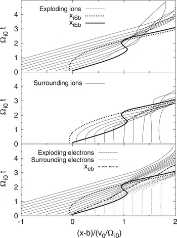
Trajectories of exploding ions, surrounding ions and electrons. After
 $x_{iEb}$
has been considerably decelerated, high-density regions appear on both sides of
 $x_{eb}$
. Reproduction of figure 3 in Yamauchi & Ohsawa (Reference Yamauchi and Ohsawa2007).

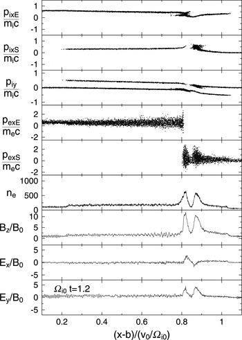
Ion and electron phase spaces and field profiles. Here,
 $p$
denotes the momentum. The two pulses seen in the field profiles reflect exploding ions to the left and surrounding ions to the right. Reproduction of figure 7 in Yamauchi & Ohsawa (Reference Yamauchi and Ohsawa2007).

As mentioned in § 1, the ions can be viewed as unmagnetized in the early phase (
 $\unicode[STIX]{x1D6FA}_{i0}t\ll 1$
), while the electrons are magnetized and move primarily with the
 $\boldsymbol{E}\times \boldsymbol{B}$
drift. Since the density
 $n$
of the exploding plasma is high (
 $n_{E}=2n_{S}$
for the case shown here, where the subscripts
 $E$
and
 $S$
indicate the exploding and surrounding plasmas, respectively), its motion across the magnetic field induces an electric field in the
 $y$
direction. Thus, in the regions where the exploding ions are present, electrons move in the
 $x$
direction with the
 $E_{y}\times B_{z}$
drift.
Figure 3, which is figure 3 in YO’s 2007 paper, shows trajectories of exploding ions, surrounding ions and electrons. The three thick lines
 $x_{iEb}$
,
 $x_{iSb}$
, and
 $x_{eb}$
represent the trajectories of particles that were initially at the boundary
 $x=b$
. Roughly speaking,
 $x_{iEb}$
shows the motion of the front of the exploding ions and
 $x_{iSb}$
the rear end of the surrounding ions. In the early phase,
 $x_{iEb}$
goes ahead of
 $x_{iSb}$
and
 $x_{eb}$
, which indicates the penetration of the exploding ions into the surrounding plasma. The surrounding ions that have been overtaken by the front part of the exploding ions are accelerated in the
 $y$
direction by the induced
 $E_{y}$
. However, owing to the magnetic force, the velocity of the exploding ions in the front part and that of the surrounding ions in the rear end part both soon change their directions, and thus
 $\text{d}x_{iEb}/\text{d}t$
goes down and
 $\text{d}x_{iSb}/\text{d}t$
goes up; as a result,
 $x_{iSb}$
passes
 $x_{iEb}$
at
 $\unicode[STIX]{x1D6FA}_{i0}t=2.1$
. During the time
 $\unicode[STIX]{x1D6FA}_{i0}t\simeq 1.5$
through
 $\unicode[STIX]{x1D6FA}_{i0}t\simeq 2$
, the exploding ions in the front part move backward (
 $\text{d}x_{iEb}/\text{d}t$
becomes negative), and on both sides of
 $x_{eb}$
there appear high-density regions, where ion and electron trajectories are concentrated. These are magnetosonic pulses moving away from each other, one propagating forward (to the right) in the surrounding plasma and the other backward (to the left) in the exploding plasma.
Figure 4, which is figure 7 in YO’s 2007 paper, displays ion and electron phase space plots and density and field profiles at
 $\unicode[STIX]{x1D6FA}_{i0}t=1.2$
. These profiles have two noticeable peaks, which are the forward (right-going) and backward (left-going) magnetosonic pulses. Although they are both in the region
 $x>x_{eb}(t)$
at this moment (see the fourth to the sixth panels in figure 4), the left pulse soon enters the region of the exploding plasma. The right pulse eventually passes the front of the exploding ions (figures 8 and 9 of YO’s 2007 paper). The ion phase space plots show that some exploding ions are reflected backward by the left pulse and some surrounding ions forward by the right pulse.
The two pulses have grown from a wide, gentle bump in the region
 $x_{eb}<x<x_{iEb}$
(Yamauchi & Ohsawa Reference Yamauchi and Ohsawa2007, figure 5). As the magnetic field in the bump is further compressed, it begins to reflect exploding ions to the left and surrounding ions to the right. This leads to the splitting of the pulse into two.
3 Summary and discussion
Comparing the two different simulations, one for the study of practicality of magnetic compression for plasma density control for plasma-based accelerators (Gueroult & Fisch Reference Gueroult and Fisch2016) and the other for the study of shock formation processes arising from an explosion in an interstellar, collisionless plasma (Yamauchi & Ohsawa Reference Yamauchi and Ohsawa2007), we have found strong similarities in their plasma phenomena. Ions reflected by the shock wave for plasma compression generate a magnetic bump, and exploding ions penetrating the surrounding plasma also create a bump. In both cases, the bump forms around the time
 $\unicode[STIX]{x1D6FA}_{i0}t\sim 1$
near the front of the beam. In YO’s simulations, because the ion beam is quite intense, the bump further grows and reflects exploding ions backward and surrounding ions forward; as a result, the bump evolves into backward and forward magnetosonic pulses.
The results of YO’s simulations suggest that the bump in GF’s simulations would grow to a magnetosonic pulse; or it might already have developed to a magnetosonic pulse. If GF’s beam of reflected ions is more intense, it would produce a greater pulse that would affect nearby particles more strongly.
Finally, we discuss the effect of the values of basic simulation parameters such as
 $m_{i}/m_{e}$
and
 $c/v_{Te}$
. Generally speaking, if we interpret simulation results without theories, it could be dangerous. It is desirable that we have or create reliable theories that quantitatively explain simulation results. In the present case, we have nonlinear theories of magnetosonic waves based on the two-fluid model, which contains
 $m_{i}$
and
 $m_{e}$
in the basic equations. The wave properties predicted by these theories are valid for a wide range of
 $m_{i}/m_{e}$
; even the magnetosonic waves in electron–positron plasmas with
 $m_{i}/m_{e}=1$
have been studied (Takahashi, Sato & Ohsawa Reference Takahashi, Sato and Ohsawa2008). Furthermore, our acceleration theories are based on these wave theories, thus they are also valid for a wide range of
 $m_{i}/m_{e}$
. The simulation results have been quantitatively compared with these wave and particle acceleration theories (Ohsawa Reference Ohsawa2014).
The parameters
 $m_{i}/m_{e}=100$
and
 $c/v_{Te}=4$
are used in YO’s 2007 paper while
 $m_{i}/m_{e}=1846$
and
 $c/v_{Te}=1.7\times 10^{2}$
in GY’s 2016 paper. Bearing this in mind, let us look at the effect of these parameters more specifically.
One of the important effects of large
 $m_{i}/m_{e}$
is that it makes the gyroradius
 $\unicode[STIX]{x1D70C}_{i}$
of reflected ions large, compared with, say, the shock width, which is
 ${\sim}c/\unicode[STIX]{x1D714}_{pe}$
. (This
 $\unicode[STIX]{x1D70C}_{i}$
also depends on other quantities such as shock strength and magnetic-field strength. We fix those values here.) The speed of reflected ions, which is approximately
 $2v_{sh}$
, is of the order of the Alfvén speed, and thus their gyroradius is
 $\unicode[STIX]{x1D70C}_{i}\sim v_{A}/\unicode[STIX]{x1D6FA}_{i}$
. We therefore see that the ratio of this gyroradius to the shock width increases with
 $m_{i}/m_{e}$
:
 $\unicode[STIX]{x1D70C}_{i}/(c/\unicode[STIX]{x1D714}_{pe})=(m_{i}/m_{e})^{1/2}$
.
Similarly, if
 $c/v_{Te}$
is large, it makes the speed of reflected ions much larger than the ion thermal velocity
 $v_{Ti}$
, which can be seen from the relation
 $$\begin{eqnarray}v_{A}/v_{Ti}=(c/v_{Te})(T_{e}/T_{i})^{1/2}(|\unicode[STIX]{x1D6FA}_{e}|/\unicode[STIX]{x1D714}_{pe}).\end{eqnarray}$$
With high
 $m_{i}/m_{e}$
and
 $c/v_{Te}$
, therefore, reflected ions have large orbits in the phase space
 $(x,v_{ix})$
. Another effect of high
 $c/v_{Te}$
is that
 $f(Mv_{A})$
becomes small. However, this does not necessarily mean that
 $f(v_{ref})$
is also small. We see this from a discussion similar to the one in § 2.1 on
 $f(v_{ref})$
in low beta plasmas. Inspection of (2.2) and (3.1) shows that the magnitude of electric potential increases with
 $c/v_{Te}$
:
 $e\unicode[STIX]{x1D719}/(m_{i}v_{Ti}^{2}/2)$
is proportional to
 $(c/v_{Te})^{2}$
. The minimum velocity for reflection,
 $v_{ref}$
given by (2.1), can be comparable to
 $v_{Ti}$
even if
 $c/v_{Te}$
is large. This explains why shock waves in GF’s simulations with a high
 $c/v_{Te}$
reflect a great number of ions.
If one carries out a series of shock simulations, gradually raising
 $M$
from unity, shock waves would begin to reflect ions at some value of
 $M$
. This critical value will go up as one decreases
 $v_{Ti}$
. At the same time, however, the critical value will be lower than
 ${\sim}2$
even for small values of
 $v_{Ti}$
.
Acknowledgements
The author is grateful to Professor N. J. Fisch and Dr R. Gueroult at Princeton Plasma Physics Laboratory for stimulating discussions and for allowing him to use some of the figures in their 2016 paper. The author would also like to thank Professor S. Usami at National Institute for Fusion Science for his helpful advice on the use of LaTex for the Journal of Plasma Physics.