1. Introduction
1.1. Large-scale structures in wall-bounded turbulence
In wall-bounded turbulent flows, large-scale structures in the outer layer contribute significantly to the transfer of momentum and to the turbulent kinetic energy. These motions possess both temporal and spatial coherence, which scales with the outer length scale
 ${\it\delta}$
, where
 ${\it\delta}$
is the channel half-height, the pipe radius, or the boundary layer thickness. Large-scale motions (LSMs) are the bulges in the outer region of turbulent boundary layers with a streamwise length of the order of 1–3
 ${\it\delta}$
(Adrian Reference Adrian2007). Adrian, Meinhart & Tomkins (Reference Adrian, Meinhart and Tomkins2000) showed that LSMs are in the form of hierarchical structures of hairpin vortex packets, where the mature hairpin packets are associated with the bulges. The groups of vortices induce coherent induction and thus form relatively low-momentum zones. These structures contribute a significant fraction of the Reynolds shear stress in turbulent boundary layers (Ganapathisubramani, Longmire & Marusic Reference Ganapathisubramani, Longmire and Marusic2003; Balakumar & Adrian Reference Balakumar and Adrian2007; Lee & Sung Reference Lee and Sung2011) and internal flows (Liu, Adrian & Hanratty Reference Liu, Adrian and Hanratty2001; Guala, Hommema & Adrian Reference Guala, Hommema and Adrian2006; Balakumar & Adrian Reference Balakumar and Adrian2007; Wu, Baltzer & Adrian Reference Wu, Baltzer and Adrian2012; Lee & Sung Reference Lee and Sung2013; Ahn et al.
Reference Ahn, Lee, Lee, Kang and Sung2015).
Structures with very long streamwise extent have received particular attention. Their spectral signature was detected in the premultiplied energy spectra of turbulent pipe flow by Kim & Adrian (Reference Kim and Adrian1999). Those authors found two distinct peaks, one of which was at a wavelength significantly longer than the characteristic length of LSMs – they termed the associated structures ‘very-large-scale motions’ (VLSMs). Subsequently, experimental and numerical studies (e.g. del Álamo & Jiménez Reference del Álamo and Jiménez2003; Guala et al.
Reference Guala, Hommema and Adrian2006; Balakumar & Adrian Reference Balakumar and Adrian2007; Hutchins & Marusic Reference Hutchins and Marusic2007a
; Monty et al.
Reference Monty, Stewart, Williams and Chong2007; Lee & Sung Reference Lee and Sung2011, Reference Lee and Sung2013; Wu et al.
Reference Wu, Baltzer and Adrian2012) reported the presence of elongated turbulence structures
 $O$
(
 $6{-}20{\it\delta}$
). Guala et al. (Reference Guala, Hommema and Adrian2006) defined VLSMs as streamwise wavelengths greater than
 $3{\it\delta}$
, and computed their contributions to the streamwise turbulent energy and the Reynolds shear stress in pipe flows. Balakumar & Adrian (Reference Balakumar and Adrian2007) extended this approach to turbulent boundary layers and channel flows in order to differentiate LSMs and VLSMs. Direct numerical simulation (DNS) of 30
 ${\it\delta}$
-long turbulent pipe flow (
 $Re_{{\it\tau}}=685$
) by Wu et al. (Reference Wu, Baltzer and Adrian2012) showed a weak peak associated with VLSMs. They reported the distinct behaviour of LSMs and VLSMs in the net force spectra; the wavelength associated with LSMs decelerates the mean streamwise flow profile in the log layer while the VLSMs accelerate the flow even near the wall. Ahn et al. (Reference Ahn, Lee, Lee, Kang and Sung2015) performed a DNS of a 30
 ${\it\delta}$
-long turbulent pipe flow at
 $Re_{{\it\tau}}=3008$
, and observed a bimodal distribution with a distinct outer peak that is related to VLSMs in the premultiplied energy spectra of the streamwise velocity fluctuations and the Reynolds shear stress.
1.2. Near-wall influence of large-scale structures
A robust feature of very long motions is their influence on the near-wall region. Using DNS data of turbulent channel flow at
 $Re_{{\it\tau}}=934$
, the footprint of very long low-speed motions was shown to extend to the wall and thus maintains the large scales in the near-wall region (Hutchins & Marusic Reference Hutchins and Marusic2007a
). This near-wall impression contradicts scaling of the streamwise turbulence intensity using the friction velocity and the viscous length scale (del Álamo & Jiménez Reference del Álamo and Jiménez2003; Hoyas & Jiménez Reference Hoyas and Jiménez2006; Hutchins & Marusic Reference Hutchins and Marusic2007a
), and underscores that the large scales and the near-wall region are interlinked. Furthermore, Hutchins & Marusic (Reference Hutchins and Marusic2007b
) demonstrated that the outer large scales modulate the small-scale energy in the near-wall region. Subsequently, Mathis, Hutchins & Marusic (Reference Mathis, Hutchins and Marusic2009) quantified this influence using the Hilbert transform. They defined the amplitude modulation coefficient using the correlation between the large-scale component of the streamwise fluctuating velocity (
 $u$
) and the low-pass-filtered envelope of the small scales. The coefficient is positive in the near-wall region, which represents the top-down influence of outer large-scale structures on the near-wall region. In addition, the wall-normal and spanwise velocity fluctuations, as well as the instantaneous Reynolds shear stresses, associated with the small scales are all modulated in an analogous manner to that reported for the streamwise velocity perturbations (Talluru et al.
Reference Talluru, Baidya, Hutchins and Marusic2014).
Baltzer, Adrian & Wu (Reference Baltzer, Adrian and Wu2013) defined VLSMs as low-speed regions longer than
 $3{\it\delta}$
in a DNS of pipe flow at
 $Re_{{\it\tau}}=685$
, which is consistent with earlier definitions based on the streamwise wavelength (Guala et al.
Reference Guala, Hommema and Adrian2006; Balakumar & Adrian Reference Balakumar and Adrian2007; Wu et al.
Reference Wu, Baltzer and Adrian2012). Very long meandering motions of low-speed fluid in the log layer contribute a large fraction of the Reynolds shear stress and of the streamwise kinetic energy in turbulent flows (Hutchins & Marusic Reference Hutchins and Marusic2007a
; Monty et al.
Reference Monty, Hutchins, Ng, Marusic and Chong2009). These structures were therefore the focus of a number of previous studies that noted the dominant contribution of the Q2 (ejection) events (e.g. Ganapathisubramani et al.
Reference Ganapathisubramani, Longmire and Marusic2003; Tomkins & Adrian Reference Tomkins and Adrian2003; Lee & Sung Reference Lee and Sung2011; Baltzer et al.
Reference Baltzer, Adrian and Wu2013). These low-speed motions are, however, flanked by high-speed regions (Hutchins & Marusic Reference Hutchins and Marusic2007a
; Monty et al.
Reference Monty, Stewart, Williams and Chong2007) which also contribute to the Reynolds shear stress through the Q4 (sweep) events. Dennis & Nickels (Reference Dennis and Nickels2011) evaluated the length and wall-normal extent of both the very-long low- and high-speed structures. The distribution of the latter was similar to that of low-speed streaks, but relatively shorter in streamwise extent. A similar trend was reported by Lee & Sung (Reference Lee and Sung2013) and Sillero, Jiménez & Moser (Reference Sillero, Jiménez and Moser2014) who compared the streamwise and spanwise length scales of the high- and low-momentum regions. In addition, large-scale positive-
 $u$
events amplify near-wall small-scale energy but the negative-
 $u$
events attenuate the small-scale fluctuations (Hutchins & Marusic Reference Hutchins and Marusic2007b
; Mathis et al.
Reference Mathis, Hutchins and Marusic2009; Ganapathisubramani et al.
Reference Ganapathisubramani, Hutchins, Monty, Chung and Marusic2012). These observations suggest different near-wall influence of low- and high-speed regions associated with LSMs and VLSMs – the footprint effects that are explored in the present study.
1.3. Organization of large-scale structures with outer roll cells
Although the role of large-scale structures in wall-bounded turbulence can be quantified using conventional statistical measures, e.g. in terms of their contribution to the Reynolds stresses, their dynamics remain the subject of active research. Kim & Adrian (Reference Kim and Adrian1999) conjectured that VLSMs are the concatenation of LSMs in the form of hairpin vortex packets. Using time-resolved instantaneous flow fields from DNS of a turbulent boundary layer (
 $Re_{{\it\tau}}=850$
), Lee & Sung (Reference Lee and Sung2011) presented evidence in support of that mechanism. In a later study, Baltzer et al. (Reference Baltzer, Adrian and Wu2013) showed the concatenation of LSMs with extended streamwise alignment and along preferred azimuthal offset to form VLSMs in DNS of pipe flow (
 $Re_{{\it\tau}}=685$
). Alternative views include that VLSMs arise from a linear amplification mechanism (del Álamo & Jiménez Reference del Álamo and Jiménez2006; McKeon & Sharma Reference McKeon and Sharma2010), and that LSMs and VLSMs can self-sustain autonomously (Hwang & Cossu Reference Hwang and Cossu2010). In this work, we focus on the genesis of VLSMs from the concatenation of LSMs. Recently, Lee et al. (Reference Lee, Lee, Choi and Sung2014) examined the spatial and temporal relationship between LSMs and VLSMs statistically. They found that the low-speed streaks with length 1–3
 ${\it\delta}$
in the outer region undergo merging. The merging process is facilitated by the difference in convection speed, which depends on the magnitude of the streamwise velocity fluctuations,
 $u$
. The results by Lee et al. (Reference Lee, Lee, Choi and Sung2014) motivate a detailed analysis of the merging process starting from its precursors through its completion and its impact on the near-wall dynamics. The connection between the outer large scales and the near-wall motions was explored by Toh & Itano (Reference Toh and Itano2005) in the streamwise minimal channel at
 $Re_{{\it\tau}}=349$
. They reported that the large-scale outer structures are situated between a pair of large-scale circulations, and induce a collective aggregation of low-speed near-wall streaks. In turn, the intense near-wall motions reach up and can potentially have a bottom-up influence on the strength of outer velocity fluctuations (Adrian Reference Adrian2007). Based on evidence from several instantaneous cross-stream flow fields, Mito et al. (Reference Mito, Hanratty, Zandonade and Moser2007) pointed out the vortices in the log layer, which could lift fluid upwards and establish this bottom-up effect.
The presence of large-scale circulations, or roll cells, in the conditional averages of turbulent channel flow data (
 $Re_{{\it\tau}}=934$
) was also reported by Hutchins & Marusic (Reference Hutchins and Marusic2007b
). The conditional average based on the negative-
 $u$
event showed the presence of a counter-rotating roll mode, and that the amplitude of small scales was strongly connected with the large-scale structures. Chung & McKeon (Reference Chung and McKeon2010) also found a similar counter-rotating circulation on either side of the large-scale low-speed events in the conditionally averaged fields of large-eddy simulations of channel flow. They noted that the outer and near-wall regions of the flow are interlinked through the roll-cell patterns. The counter-rotating circulations were examined by Baltzer et al. (Reference Baltzer, Adrian and Wu2013) who analysed turbulent pipe flow using conditional averaging and proper orthogonal decomposition. The roll-cell motions centred above the log layer were attributed to the preferred spanwise offset of LSMs that concatenated to form long low-momentum regions along a helical angle of
 $4^{\circ }{-}8^{\circ }$
. These earlier studies thus conjectured that the large-scale circulation in the outer region is associated with the large-scale structures as well as the intense near-wall velocity fluctuations which, in turn, potentially have a bottom-up influence on the outer dynamics – an interaction that is examined in detail in the present study.
The objective of the present study is to investigate the influence of low- and high-speed large-scale structures on the near-wall region by focusing on their associated large-scale circulations. We examine the induced dispersive or congregative near-wall motions, and the connection of this process to the formation of long low-speed structures in the log layer. Our approach relies on the analysis of data from DNS of turbulent channel flow at
 $Re_{{\it\tau}}=930$
in a long computational domain of length
 $10{\rm\pi}{\it\delta}$
, which is sufficient for the study of very long structures. A brief description of the computational approach and the conditional sampling techniques for identifying the low- and high-speed instantaneous flow structures is provided in § 2. In § 3, the low- and high-speed structures are compared based on their spatial extent. Next, those structures associated with LSMs and VLSMs are examined using the conditional two-point correlations to reveal the spatial relationship with the surrounding velocity perturbations. We then perform conditional sampling of the footprints of wall-attached large-scale structures to see the impact on the near-wall region. The evolutions of near-wall and outer structures are reported based on instantaneous flow fields, with particular focus on their interaction, which facilitates merging of the large outer scales. Finally, a summary of the main findings is provided in § 4.
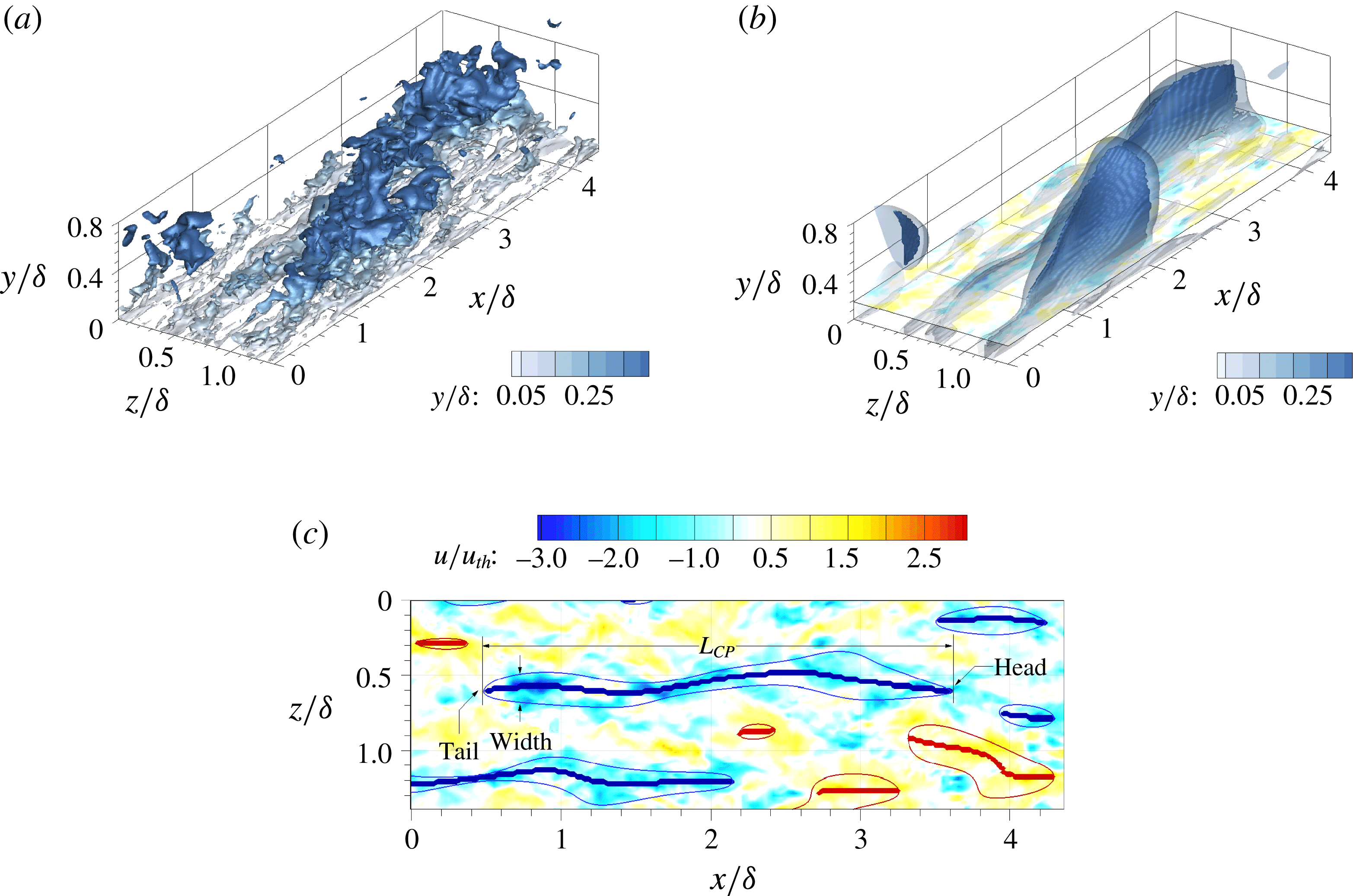
Isosurfaces of (a) the negative streamwise velocity fluctuations (
 $u=-u_{th,raw}$
) and (b) the Gaussian and long-wavelength-pass-filtered flow field (
 $\hat{u} =-u_{th}$
) with the characteristic projections (
 $CP$
). (c) The wall-parallel plane
 $y/{\it\delta}=0.15$
at the same instance as frame (b); the thick and thin blue (red) lines represent the
 $CP=-1$
(
 $CP=+1$
) and
 $\hat{u} =-u_{th}$
(
 $\hat{u} =+u_{th}$
), respectively.

2. Numerical details
2.1. Direct numerical simulation
The Navier–Stokes equations for incompressible flow are solved using the fully implicit decoupling method by Kim, Baek & Sung (Reference Kim, Baek and Sung2002). The configuration corresponds to fully developed turbulent channel flow, and details of the DNS and the validation are provided in the earlier study by Lee et al. (Reference Lee, Lee, Choi and Sung2014). In the present study,
 $x$
,
 $y$
and
 $z$
denote the streamwise, wall-normal and spanwise directions, respectively, and the associated components of velocity fluctuations are
 $u$
,
 $v$
and
 $w$
; capital letters are used to indicate mean quantities. An angle bracket
 $\langle \cdot \rangle$
denotes ensemble averaging. The superscript
 $+$
represents quantities normalized by the viscous scales, namely the friction velocity,
 $u_{{\it\tau}}$
, and viscosity,
 ${\it\nu}$
. The Reynolds number based on the channel half-height,
 ${\it\delta}$
, and the laminar centreline velocity,
 $U_{CL}$
, is
 $Re_{{\it\delta}}=28\,000$
, and the friction Reynolds number is
 $Re_{{\it\tau}}=930$
. The domain size in the streamwise and spanwise directions is
 $(L_{x},L_{z})=(10{\rm\pi}{\it\delta},3{\rm\pi}{\it\delta})$
. A staggered mesh is employed with
 $4993\times 401\times 2497$
grid points in the
 $x$
,
 $y$
and
 $z$
directions, respectively. The grid sizes in the homogeneous directions are
 ${\rm\Delta}x^{+}=5.86$
and
 ${\rm\Delta}z^{+}=3.51$
. The minimum and maximum wall-normal grid spacings are
 ${\rm\Delta}y_{min}^{+}=0.0287$
and
 ${\rm\Delta}y_{max}^{+}=7.31$
, respectively. The simulation is performed at a constant mass flow rate, and the time step is
 ${\rm\Delta}t=0.002{\it\delta}/U_{CL}$
, or
 ${\rm\Delta}t^{+}=0.0618$
, and the averaging period spans
 $220{\it\delta}/U_{CL}$
, corresponding to seven sweeps across the flow domain. A total of 2010 snapshots are stored, with each two consecutive fields separated by
 $0.1{\it\delta}/U_{CL}$
(or
 ${\rm\Delta}t^{+}=3.09$
). In the present study, the following wall-normal regions are defined: the near-wall region
 $y^{+}<30$
; the log layer
 $30<y^{+}<0.15{\it\delta}^{+}$
; and the channel core
 $y^{+}>0.15{\it\delta}^{+}$
.
2.2. Structure-detection method
To investigate the formation of elongated
 $u$
structures in space and time, streak detection and conditional sampling techniques are applied to the instantaneous fields. The streak-detection algorithm is based on the work by Nolan & Zaki (Reference Nolan and Zaki2013), where local extrema of
 $u$
are used to reconstruct the three-dimensional (3D) streamwise-elongated structures. Further detailed descriptions of the methodology can be found in Zaki (Reference Zaki2013). Figure 1 displays an example of the outcome of the detection method. The threshold
 $u_{th,raw}=0.1U_{b}$
, where
 $U_{b}$
is the bulk velocity, is used in the present study (Dennis & Nickels Reference Dennis and Nickels2011; Baltzer et al.
Reference Baltzer, Adrian and Wu2013; Lee et al.
Reference Lee, Lee, Choi and Sung2014). The procedure is outlined below.
Step 1: Gaussian filter. A two-dimensional Gaussian filter is applied in the
 $y$
–
 $z$
plane to the instantaneous
 $u$
field. The standard deviation (
 ${\it\sigma}$
) of the Gaussian filter is determined as a function of the wall-normal distance, because the spanwise length scale of the
 $u$
motions varies with height from the wall. The standard deviation is set to the half-width of the spanwise two-point correlation of
 $u$
at a level of 0.5. This choice prevents adjacent negative
 $u$
from counterbalancing the positive
 $u$
, and vice versa. The curve-fitted standard deviation function
 ${\it\sigma}(y/{\it\delta})$
is
 $$\begin{eqnarray}{\it\sigma}/{\it\delta}=0.1513(y/{\it\delta})^{3}-0.5142(y/{\it\delta})^{2}+0.4992(y/{\it\delta})+0.0176.\end{eqnarray}$$
Step 2: Long-wavelength-pass filter. A long-wavelength-pass filter is applied to the Gaussian-filtered flow fields in order to isolate structures longer than
 $1{\it\delta}$
in the streamwise direction. If the streamwise filter is applied alone, it leads to discontinuous isosurfaces of the velocity field, which are not suitable for identifying contiguous
 $u$
structures along the streamwise direction (Lee et al.
Reference Lee, Lee, Choi and Sung2014). Hence, the Gaussian filter is also needed in order to ensure that the
 $u$
isosurfaces are smooth.
The smoothed isosurfaces in figure 1(b) illustrate the filtered flow field,
 $\hat{u}$
. Owing to the weakened magnitude of
 $u$
by the filters, the velocity threshold is corrected,
 $u_{th}(y)=f(y)u_{th,raw}$
, where
 $f(y)=\langle u(\boldsymbol{x})\hat{u} (\boldsymbol{x})\rangle /\langle u(\boldsymbol{x})u(\boldsymbol{x})\rangle$
. Then local extrema are identified in the filtered fields along lines in the spanwise direction. Note that
 $\hat{u}$
is a smooth function due to the Gaussian filter and, as a result, the computed local extrema at the core of each flow structure are contiguous (see figure 14 in Lee et al. (Reference Lee, Lee, Choi and Sung2014)). Neighbouring extrema thus mark the cores of the velocity disturbances. The extrema that are connected in the streamwise direction are linked and labelled as a unique object, which can be regarded as the characteristic projections (
 $CP$
) of the flow structures. In this manner,
 $CP$
represents the streamwise and wall-normal extents of LSMs:
 $$\begin{eqnarray}CP(x,y,z)=\left\{\begin{array}{@{}ll@{}}+1 & \text{where }\partial \hat{u} /\partial z=0\text{ and }\hat{u} >u_{th},\\ -1 & \text{where }\partial \hat{u} /\partial z=0\text{ and }\hat{u} <-u_{th},\\ 0 & \text{otherwise}.\end{array}\right.\end{eqnarray}$$
Based on the above definition,
 $CP=+1$
marks high-speed structures and
 $CP=-1$
identifies low-speed ones. Figure 1(b) shows a transparent isosurface of the filtered velocity field, along with the surface
 $CP=-1$
coloured by wall-normal height. Figure 1(c) shows a top view of the
 $u$
-perturbation contours at
 $y/{\it\delta}=0.15$
. The thick solid lines show the intersection of the wall-parallel plane with the
 $CP$
surface and they mark the streamwise and spanwise positions of the organized motion. The most downstream and upstream ends of
 $CP$
denote the head and the tail of the streak, respectively. The streamwise length,
 $L_{CP}$
, of each streak is measured and the spanwise boundary of the streak is defined by identifying lower and upper bounds (
 $\hat{u} =\pm u_{th}$
) on either side of the streak core (see figure 1
c). If there are multiple adjacent streaks (for example, near
 $x/{\it\delta}=4{-}6$
in figure 3
b), the boundaries of each streak are adjusted to the spanwise location where
 $\partial \hat{u} /\partial z$
changes sign.
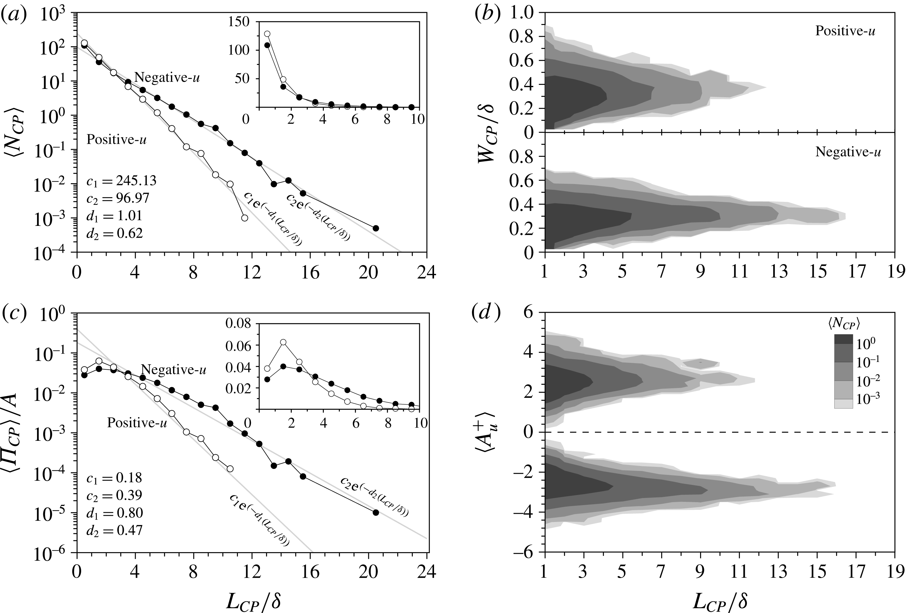
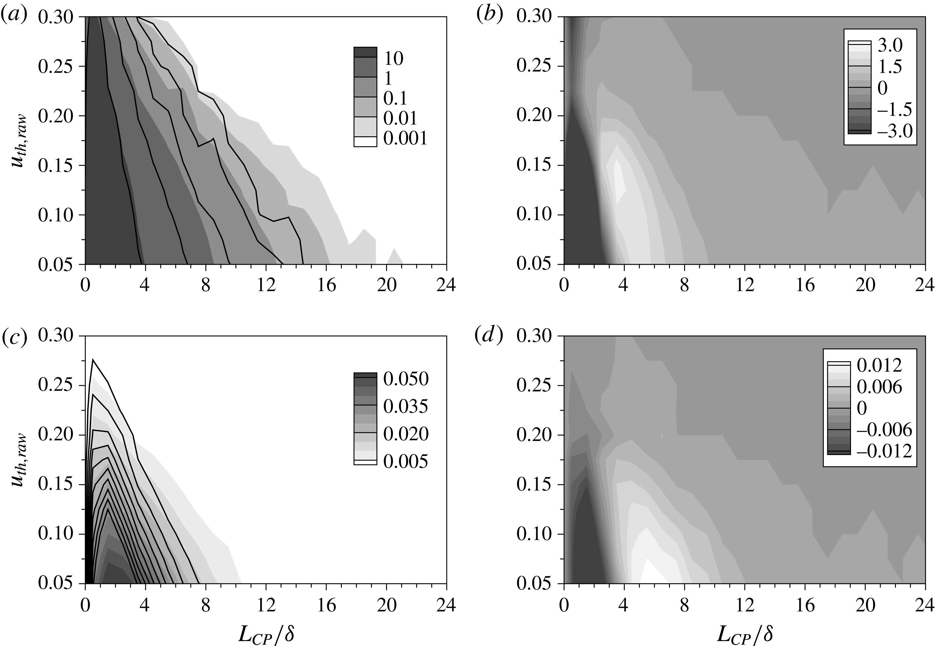
Histograms of the streamwise length (
 $L_{CP}$
) of low- and high-speed streaks at
 $y/{\it\delta}=0.15$
. (a) The mean number of the streaks per field (
 $\langle N_{CP}\rangle$
) in the wall-parallel plane. (b) The spanwise width (
 $W_{CP}$
) of low- and high-speed streaks. (c) The mean area occupied by the structures per field (
 $\langle {\it\Pi}_{CP}\rangle$
) versus their streamwise length;
 $\langle {\it\Pi}_{CP}\rangle$
is normalized by the total area of the wall-parallel plane (
 $A=L_{x}\times L_{z}$
). (d) The mean amplitude (
 $A_{u}$
) of the low- and high-speed streaks of a particular length. In (a,c), the closed and open symbols represent low- and high-speed streaks, respectively. The grey lines mark an exponential curve fit, and the insets show the results in linear scale. In (b,d), the contour lines indicate
 $\langle N_{CP}\rangle$
. The bin size for
 $L_{CP}$
is
 $1{\it\delta}$
.

3. Results and discussion
3.1. Long streaks of streamwise velocity fluctuations
In this section, the length and area of long negative- and positive-
 $u$
regions are examined using the structure-detection algorithm (§ 2.2). Figure 2 shows the populations of negative- and positive-
 $u$
structures versus their streamwise length,
 $L_{CP}$
, at
 $y/{\it\delta}=0.15$
. The mean number (
 $\langle N_{CP}\rangle$
) of negative-
 $u$
(closed symbol) and positive-
 $u$
(open symbol) regions is displayed in figure 2(a). A single occurrence,
 $\langle N_{CP}\rangle =1$
, means that an average of one structure with the specified length is observed in this wall-parallel plane per unit time. Structures that are recorded more than once per field have a streamwise length less than
 $8{\it\delta}$
for the negative-
 $u$
regions and
 $6{\it\delta}$
for the positive counterparts. The vast majority of detected streaks have a streamwise length less than
 $1{\it\delta}$
. The maximum streamwise extent of negative-
 $u$
regions is approximately
 $20{\it\delta}$
, while that of positive structures is only
 $12{\it\delta}$
. Although the populations of both negative- and positive-
 $u$
regions decrease logarithmically with their length, the negative-
 $u$
regions tend to be longer than their positive counterparts and the latter are relatively biased towards shorter lengths. Beyond 3
 ${\it\delta}$
in particular, the disparity between the populations of low and high speed becomes more pronounced. The slope of the populations,
 $d_{i}$
, is found to be steeper for positive-
 $u$
regions, where
 $d_{1}=1.01$
and
 $d_{2}=0.62$
for positive and negative
 $u$
, respectively. The results based on the present detection algorithm are in agreement with those by Dennis & Nickels (Reference Dennis and Nickels2011) and by Baltzer et al. (Reference Baltzer, Adrian and Wu2013) despite the difference in the structure identification procedure. Dennis & Nickels (Reference Dennis and Nickels2011) counted both low- and high-speed structures whose streamwise lengths were greater than
 $2{\it\delta}$
in a turbulent boundary layer. For low-speed structures, 44 % of the structures were below 3
 ${\it\delta}$
while 54 % of the high-speed structures were in the same range. The distributions evaluated using the present algorithm show similar trends: 43 % and 60 % for low- and high-speed regions, respectively. The predicted ratio of long low- and high-speed structures (
 ${>}2{\it\delta}$
) are also similar in the two studies, approximately 1.3–1.5. Low-speed regions that are longer than
 $7{\it\delta}$
are less than 5 % of the total population, consistent with Baltzer et al. (Reference Baltzer, Adrian and Wu2013).
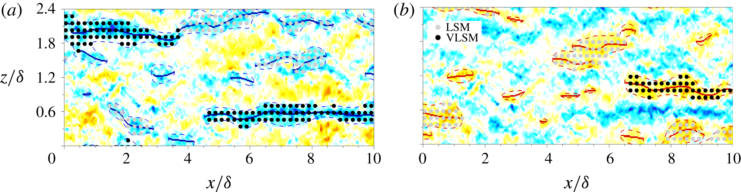
Area identification at
 $y/{\it\delta}=0.15$
: (a) nLSM (
 $u_{1}$
) and nVLSM (
 $u_{2}$
); (b) pLSM (
 $u_{3}$
) and pVLSM (
 $u_{4}$
); here n = negative and p = positive. The contour levels are the same as in figure 1(c). The solid and dashed lines represent
 $CP=\pm 1$
and
 $\hat{u} =\pm u_{th}$
, respectively.

The population trends of the positive- and negative-
 $u$
regions classified based on their streamwise length (
 $L_{CP}$
) and spanwise width (
 $W_{CP}$
) are displayed in figure 2(b). The width of each region is computed by measuring lower and upper bounds along
 $CP=\pm 1$
(see figure 1),
 $$\begin{eqnarray}W_{CP}(L_{CP})=\frac{1}{L_{CP}}\int _{z_{1}}^{z_{2}}\!\int _{tail}^{head}{\it\zeta}(x,z;L_{CP})\,\text{d}x\,\text{d}z,\end{eqnarray}$$
where
 $z_{1}$
and
 $z_{2}$
are lower and upper bounds along
 $CP=\pm 1$
and
 $$\begin{eqnarray}{\it\zeta}(x,z;L_{CP})=\left\{\begin{array}{@{}ll@{}}1, & \text{if }|\hat{u} |>u_{th},\\ 0, & \text{otherwise.}\end{array}\right.\end{eqnarray}$$
The contour lines represent
 $\langle N_{CP}\rangle$
and only streaks with length greater than
 $1{\it\delta}$
are shown. As the length of the streaks increases, the streaks maintain their spanwise width around
 $0.3{\it\delta}$
. While the most probable width of positive- and negative-
 $u$
streaks remains comparable,
 $W_{CP}\approx 0.3{\it\delta}$
, the maximum width of negative-
 $u$
streaks is generally narrower than its positive-
 $u$
counterpart. The width of short positive-
 $u$
streaks (
 ${<}3{\it\delta}$
) reaches up to
 $0.8{\it\delta}$
. In general, the positive-
 $u$
streaks are shorter and wider than the negative-
 $u$
ones. To analyse the spatial extent occupied by the positive- and negative-
 $u$
structures, figure 2(c) shows the mean area
 $\langle {\it\Pi}_{CP}\rangle$
of the streaks in the
 $y/{\it\delta}=0.15$
plane. The area occupied by streaks of a particular length
 ${\it\Pi}_{CP}(L_{CP})$
is defined as
 $$\begin{eqnarray}{\it\Pi}_{CP}(L_{CP})=\mathop{\sum }_{i=1}^{N_{CP}}A_{i}(L_{CP}),\end{eqnarray}$$
where
 $A_{i}$
is the area for each streak,
 $$\begin{eqnarray}A_{i}(L_{CP})=\int _{z_{1}}^{z_{2}}\!\int _{tail}^{head}{\it\zeta}(x,z;L_{CP})\,\text{d}x\,\text{d}z.\end{eqnarray}$$
The area
 ${\it\Pi}_{CP}$
is normalized by the total area of the wall-parallel plane (
 $A=L_{x}\times L_{z}$
). The sum of
 ${\it\Pi}_{CP}$
indicates the total area fraction occupied by streamwise velocity fluctuations greater than the threshold value. The area fraction of the weak region, where the perturbation field is weaker than the threshold value, is not included here. The total area fractions of the negative and positive
 $u$
are similar in the log layer,
 $21\,\%$
and
 $19\,\%$
, respectively, although the area fractions depend on the streamwise length of the structures. Each short-length streak has a smaller area compared to the longer streaks while
 ${\it\Pi}_{CP}$
for short-length structures is greater than the longer structures due to the higher number density in the flow field. The area fraction has a peak between
 $1{\it\delta}$
and
 $3{\it\delta}$
. In addition, the area fraction of the positive-
 $u$
regions crosses the negative counterpart around
 $L_{CP}=3{\it\delta}$
, similar to the trend of their respective populations reported in figure 2(a). Owing to the smaller population of the positive-
 $u$
regions (
 ${>}3{\it\delta}$
), their area fraction rapidly drops in comparison to the negative-
 $u$
structures. The slopes of the area fraction are
 $d_{1}=0.80$
and
 $d_{2}=0.47$
for positive and negative
 $u$
, respectively. Moreover, the area fraction of the negative-
 $u$
regions with lengths longer than
 $3{\it\delta}$
is approximately
 $10\,\%$
(
 $11\,\%$
for
 $L_{CP}<3{\it\delta}$
) and of the positive counterparts is
 $5\,\%$
(
 $14.5\,\%$
for
 $L_{CP}<3{\it\delta}$
). Although the population of long negative-
 $u$
structures is small (logarithmic decrease in their population in figure 2
a), they occupy a similar area fraction as the shorter structures. On the other hand, the area of the positive-
 $u$
regions is mainly occupied by the relatively short structures (
 $L_{CP}<3{\it\delta}$
) at
 $y/{\it\delta}=0.15$
. It should be noted that the effect of the threshold
 $u_{th}$
employed in our structure identification was examined (see Appendix). We found that the general trends reported in this section remain qualitatively unchanged.
To compare the magnitude of the streamwise velocity fluctuations within the organized motions, the strength of the streamwise streaks was evaluated along
 $L_{CP}$
. The mean amplitude for each streak,
 $A_{u}$
, is
 $$\begin{eqnarray}A_{u}(L_{CP},y)=\frac{1}{L_{CP}}\int _{tail}^{head}u|_{CP=\pm 1}\,\text{d}x.\end{eqnarray}$$
The distributions of
 $A_{u}(L_{CP},y^{+}=0.15{\it\delta}^{+})$
are shown in figure 2(d). The contours at
 $A_{u}>0$
illustrate the distribution of the positive-
 $u$
streaks and those of the negative-
 $u$
streaks are shown as
 $A_{u}<0$
. Both distributions are relatively wider for the shorter length and become narrower as the length of the streaks increases. Although the distributions of the streak amplitudes are similar for both negative and positive
 $u$
, the long streaks (
 ${\geqslant}12{\it\delta}$
) are only observed in negative
 $u$
. In addition, these long streaks carry significantly higher disturbance amplitude (
 $|A_{u}^{+}|\approx 3$
) compared with
 $u_{rms}^{+}=1.87$
at
 $y/{\it\delta}=0.15$
. Their long streamwise extent indicates that the very long-
 $u$
regions contribute a significant fraction of the Reynolds stresses.
The VLSMs are motions whose streamwise wavelengths are greater than 3
 ${\it\delta}$
(Guala et al.
Reference Guala, Hommema and Adrian2006; Balakumar & Adrian Reference Balakumar and Adrian2007; Wu et al.
Reference Wu, Baltzer and Adrian2012). Several studies have therefore used the energy contained within this wavelength range to differentiate LSMs and VLSMs (Dennis & Nickels Reference Dennis and Nickels2011; Baltzer et al.
Reference Baltzer, Adrian and Wu2013; Lee et al.
Reference Lee, Lee, Choi and Sung2014; Lee, Ahn & Sung Reference Lee, Ahn and Sung2015). In particular, Baltzer et al. (Reference Baltzer, Adrian and Wu2013) defined the VLSMs as the negative-
 $u$
streaks longer than 3
 ${\it\delta}$
at
 $y/{\it\delta}=0.15$
, and their contribution to the Reynolds shear stress at that wall-normal position was computed by Lee & Sung (Reference Lee and Sung2011, Reference Lee and Sung2013). In the present study, streamwise-extended regions of contiguous
 $CP$
in the
 $x$
–
 $z$
plane (
 $y/{\it\delta}=0.15$
) were classified into LSM and VLSM using a
 $3{\it\delta}$
limit, and these motions were further differentiated according to their sign (n
 $=$
negative and p
 $=$
positive). This classification yields the following four categories (Lee et al.
Reference Lee, Ahn and Sung2015): nLSM (
 $1{\it\delta}\leqslant L_{CP}|_{CP=-1}<3{\it\delta}$
); nVLSM (
 $L_{CP}|_{CP=-1}\geqslant 3{\it\delta}$
); pLSM (
 $1{\it\delta}\leqslant L_{CP}|_{CP=+1}<3{\it\delta}$
); and pVLSM (
 $L_{CP}|_{CP=+1}\geqslant 3{\it\delta}$
). Figure 3 shows an example of these
 $u$
structures. For convenience, we introduce an area indicator
 $I(x,z)$
, which represents the bounded area of each motion based on its sign and length:
 $$\begin{eqnarray}I(x,z)=\left\{\begin{array}{@{}l@{}}1\quad \text{where }{\it\zeta}(x,z;L_{CP})|_{nLSM}=1,\\ 2\quad \text{where }{\it\zeta}(x,z;L_{CP})|_{nVLSM}=1,\\ 3\quad \text{where }{\it\zeta}(x,z;L_{CP})|_{pLSM}=1,\\ 4\quad \text{where }{\it\zeta}(x,z;L_{CP})|_{pVLSM}=1.\end{array}\right.\end{eqnarray}$$
The velocity perturbations associated with each motion can thus be conditionally sampled based on the area indicator
 $I$
. For example, the streamwise velocity fluctuation
 $u$
corresponding to the specific motion (
 $I$
) is expressed as
 $u_{I}(x,z;y_{ref})=u(x,y_{ref},z)\mid I(x,z)$
, where
 $y_{ref}$
is 0.15
 ${\it\delta}$
. The conditional sampling was performed using the instantaneous raw streamwise velocity fluctuations
 $u$
, and the results were differentiated into the four categories given by (3.6).
3.2. Conditional velocity correlations
The spatial characteristics of long-
 $u$
streaks are explored by computing the conditional two-point correlations. For the streamwise structures (
 $u_{I}$
) identified by the area indicator function
 $I$
, the conditional correlation coefficient
 $(R)$
with the fluctuating velocity field (
 $u_{j}$
) is defined as
 $$\begin{eqnarray}R[u_{I},u_{j}](r_{x},y,r_{z};y_{ref})=\frac{\langle u_{I}(x,z;y_{ref})u_{j}(x+r_{x},y,z+r_{z})\rangle }{{\it\sigma}_{u_{I}}(y_{ref}){\it\sigma}_{j}(y)},\end{eqnarray}$$
where the subscript
 $j$
represents different components of the velocity perturbations (
 $u,v,w$
) and
 ${\it\sigma}$
is the standard deviation. For brevity, we will refer to
 $R$
simply as the correlation. The present conditional correlations (3.7) are similar to the expression by Ganapathisubramani (Reference Ganapathisubramani2008), who studied the velocity field in the vicinity of momentum sources and sinks. The evaluation of
 $R[u_{I},u_{j}]$
reflects the fluctuating velocity field associated with the specific events (
 $u_{I}$
), which can reveal the statistical structure of the flow around the long-
 $u$
motions.
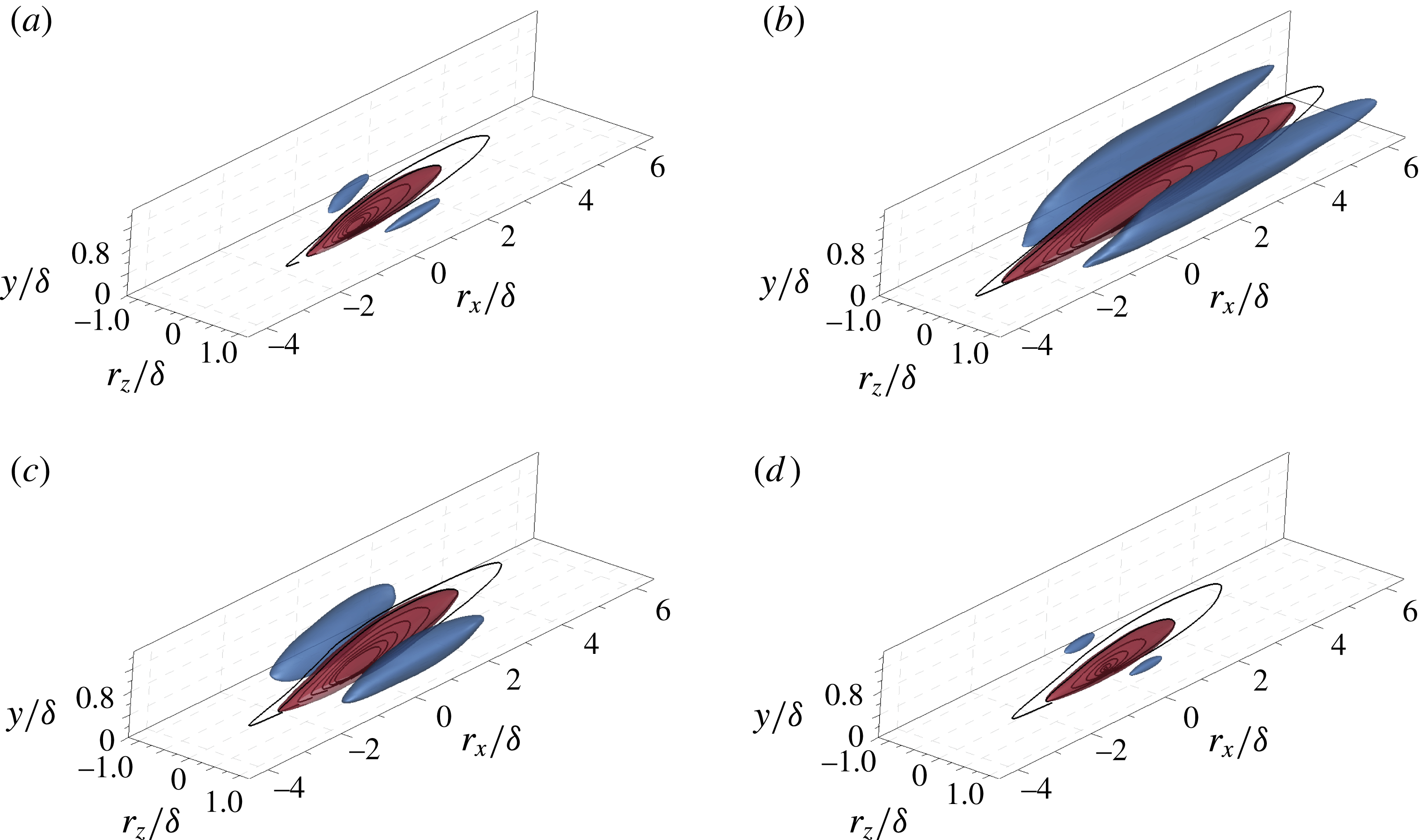
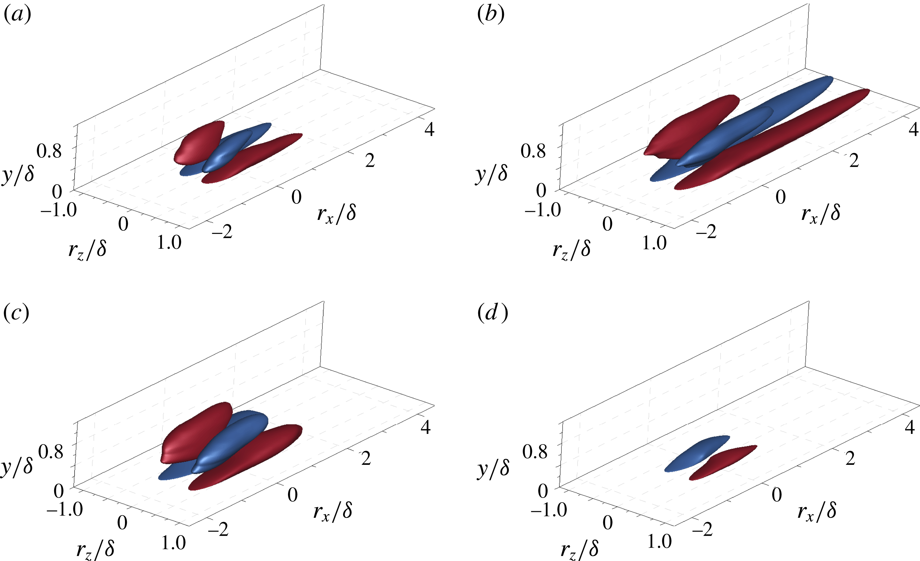
Conditional correlations of the streamwise velocity fluctuations,
 $R[u_{I},u]$
, in 3D perspective view: (a) nLSM (
 $u_{1}$
); (b) nVLSM (
 $u_{2}$
); (c) pLSM (
 $u_{3}$
); and (d) pVLSM (
 $u_{4}$
). The isosurfaces mark
 $R[u_{I},u]=0.03$
(red) and
 $-$
0.015 (blue). The inserted contour lines represent
 $R[u_{I},u]$
in the
 $x$
–
 $y$
plane (
 $r_{z}/{\it\delta}=0$
) and range from 0.02 to 0.08 with an increment of 0.01.

Figure 4 shows the 3D representation of the conditional two-point correlations
 $R[u_{I},u]$
at
 $y_{ref}/{\it\delta}=0.15$
with the contour lines in the
 $x$
–
 $y$
plane (
 $r_{z}/{\it\delta}=0$
). There is a positive isosurface of the correlations elongated in the streamwise direction and inclined with respect to the wall. The positive values have a ramp-like shape, which is a general feature of the unconditional two-point correlations (
 $R[u,u]$
) in the log layer (Hutchins & Marusic Reference Hutchins and Marusic2007a
; Lee & Sung Reference Lee and Sung2011; Baltzer et al.
Reference Baltzer, Adrian and Wu2013). Despite the general similarities to the characteristics of the unconditional correlation (
 $R[u,u]$
), the magnitude and shape of
 $R[u_{I},u]$
depend on the conditions. In particular, the correlations of nVLSM (
 $R[u_{2},u]$
) and pLSM (
 $R[u_{3},u]$
) have higher values and longer isosurfaces than the others, indicating that those structures are the most strongly correlated with the surrounding perturbation fields. The correlation of nVLSMs extends longer than that of nLSMs in the upstream and downstream directions (
 $10{\it\delta}$
and
 $6{\it\delta}$
for each case based on
 $R=0.02$
), and the maximum correlation values for nLSM and nVLSM are 0.12 and 0.17, respectively. The streamwise velocity fluctuations are more correlated with nVLSMs in both the streamwise and wall-normal directions, although the population of nVLSMs is less dominant than that of nLSMs in the log region as shown in figure 2(a). In addition, the correlation of nLSMs is inclined at a larger angle (
 ${\sim}8^{\circ }$
) in the streamwise direction compared to the nVLSMs (
 ${\sim}6^{\circ }$
). The ramp-like character of the correlations indicates that nLSMs and nVLSMs are correlated with the streamwise fluctuations in both the near-wall and core regions along the streamwise direction. The correlations are extended as footprints down to the wall and the footprint of nVLSMs is more evident than that of nLSMs. The conditional correlations of the positive-
 $u$
conditions (pLSM and pVLSM) are illustrated in figure 4(c,d). The correlations of pLSMs are more dominant than those of pVLSMs; the maximum correlation values are 0.16 and 0.09 and persist over streamwise extents of
 $7{\it\delta}$
and
 $5{\it\delta}$
, respectively. The pLSMs are organized motions of the positive-
 $u$
regions in the log layer, and this result is also consistent with the population trend and the dominant area fraction of pLSMs (14.5 %) relative to pVLSMs (5 %) at
 $y/{\it\delta}=0.15$
(figure 2
a,c).
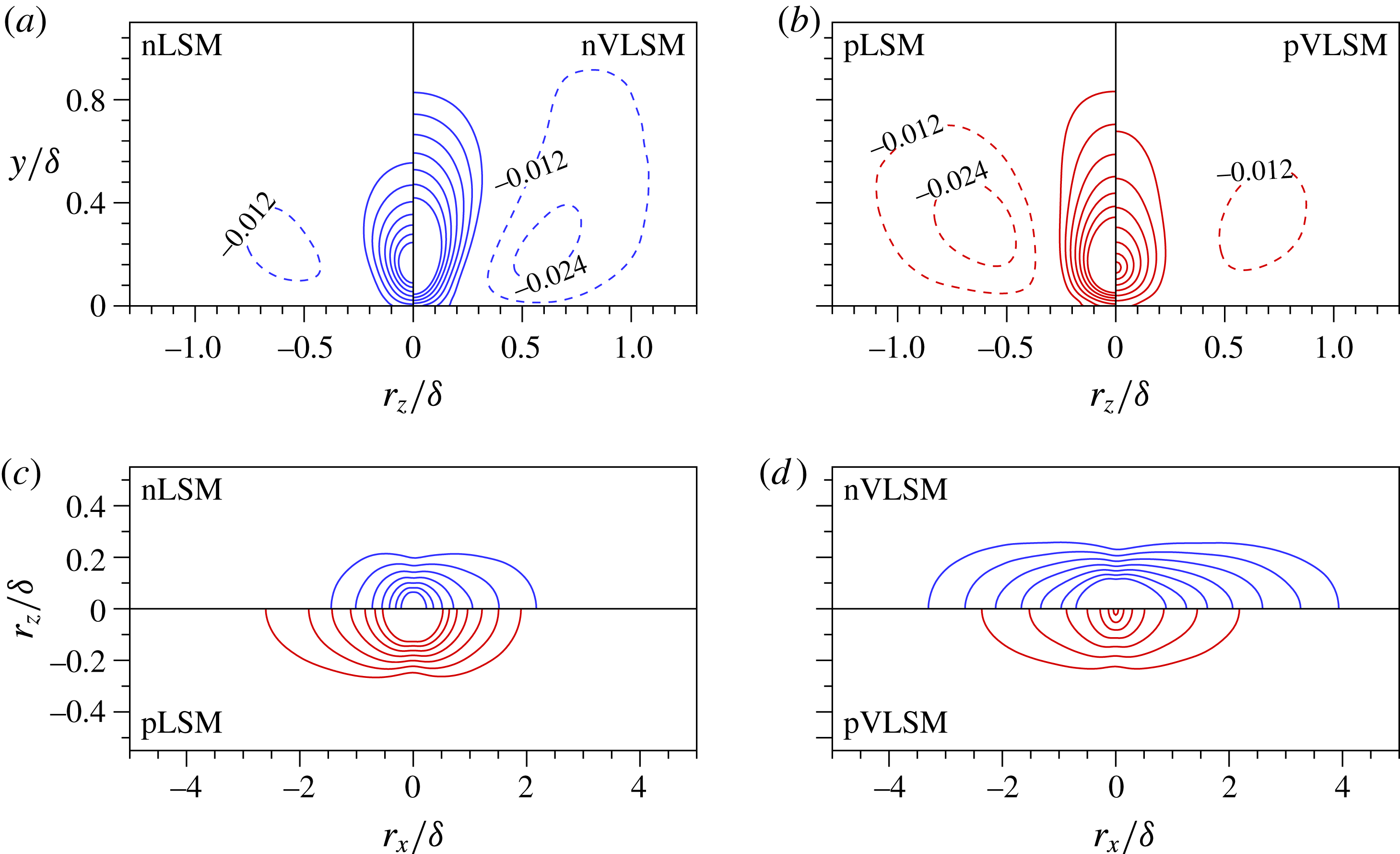
Figure 5(a,b) displays the spatial organization of the correlations in the cross-flow plane (
 $r_{x}/{\it\delta}=0$
). Note that the correlations are shown side by side in each panel, with LSMs on the left (red) and VLSMs on the right (blue) since each is symmetric in the spanwise direction. The heights of the positive correlations (
 $r_{z}/{\it\delta}=0$
) are
 $0.55{\it\delta}$
(nLSM) and
 $0.8{\it\delta}$
(nVLSM), indicating the dominance of nVLSMs up to the core region of the channel flow. The positive correlations with width
 ${\rm\Delta}z/{\it\delta}\approx 0.3$
are centred at the reference position and are flanked on both sides by weaker negative values at a distance of the order of
 $1{\it\delta}$
. The anticorrelated regions of nVLSMs are similar in height compared to the positive correlation. The distinct negative patterns observed in the correlations of nVLSMs show that relatively strong positive-
 $u$
structures are flanked on both sides of nVLSMs. A comparable spanwise size of the conditional correlations of the nLSMs and nVLSMs (
 ${\rm\Delta}z/{\it\delta}\sim 0.3$
) indicates that the two classes of structures have similar spanwise scales, which is a prerequisite for VLSMs to be formed by the streamwise concatenation of LSMs (Kim & Adrian Reference Kim and Adrian1999).
Conditional correlations
 $R[u_{I},u]$
, (a,b) in the
 $y$
–
 $z$
plane (
 $r_{x}/{\it\delta}=0$
) and (c,d) in the
 $x$
–
 $z$
plane (
 $y=y_{ref}$
): (a) nLSM (
 $u_{1}$
) and nVLSM (
 $u_{2}$
); (b) pLSM (
 $u_{3}$
) and pVLSM (
 $u_{4}$
); (c) nLSM (
 $u_{1}$
) and pLSM (
 $u_{3}$
); and (d) nVLSM (
 $u_{2}$
) and pVLSM (
 $u_{4}$
). The blue and red lines represent the negative- and positive-
 $u$
conditions. The positive contours (solid) range from 0.02 to 0.08 with an increment of 0.01 and the values of the negative contours (dashed) are reported in (a,b).

The conditional correlations of pLSMs and pVLSMs are illustrated in figure 5(b). The correlation of pLSMs reaches up to the core region similar to nVLSMs. However, the patterns of the positive-
 $u$
correlations (figure 5
b) differ appreciably in the wall-normal direction from the negative-
 $u$
correlations (figure 5
a). They retain their width along the wall-normal direction while their negative counterparts gradually decrease close to the wall. In other words, the footprint of the positive-
 $u$
structure is wider than that of the negative-
 $u$
one, which suggests that the near-wall region which is affected by the outer large scales is larger for positive-
 $u$
motions; this point will be discussed in detail in § 3.3.
Wall-parallel cross-sections (
 $y=y_{ref}$
) of the correlations are presented in figure 5(c,d). The correlations of LSMs (figure 5
c) show a bias: the pLSM is biased in the upstream direction whereas the nLSM is biased downstream. However, the correlations of VLSMs are nearly symmetric in the streamwise direction (figure 5
d). Lee & Sung (Reference Lee and Sung2013) also reported a bias in the correlation when conditioned on the sign of
 $u$
only (but not the size of the structure). The present results thus attribute this bias to the dominant contribution by
 $u$
regions with length 1–3
 ${\it\delta}$
(LSMs). In addition, the correlations that represent the prominent length scales in the streamwise and spanwise directions are pLSMs and nVLSMs (figure 5
c,d). Lee & Sung (Reference Lee and Sung2013) and Sillero et al. (Reference Sillero, Jiménez and Moser2014) used the two-point correlation to estimate the streamwise and spanwise length scales at various wall-normal locations. They found that the negative-
 $u$
structures are slightly longer and narrower than the positive-
 $u$
ones. The present correlations reveal that the relatively longer (negative-
 $u$
) and wider (positive-
 $u$
) length scales observed in those previous studies are due to the contributions of nVLSMs and pLSMs, respectively.
Conditional cross-correlations,
 $R[u_{I},w]$
, in 3D perspective view: (a) nLSM (
 $u_{1}$
); (b) nVLSM (
 $u_{2}$
); (c) pLSM (
 $u_{3}$
); and (d) pVLSM (
 $u_{4}$
). The red and blue isosurfaces are
 $R[u_{I},w]=0.01$
and
 $-0.01$
, respectively.

Next, the conditional cross-correlations between the specific
 $u$
events and the spanwise velocity fluctuations (
 $w$
),
 $R[u_{I},w]$
, are examined. The 3D representations of
 $R[u_{I},w]$
are illustrated in figure 6. Each of figures 6(a)–6(c) includes four isosurfaces, two of which are attached to the wall. Figure 6(d) for pVLSM only displays two isosurfaces due to the weak correlation level. The sign of the correlation reflects the dominant direction of spanwise velocity fluctuations associated with the
 $u$
events. For the negative-
 $u$
events, the positive correlation is associated with negative
 $w$
and the anticorrelation corresponds to positive
 $w$
. In other words, the attached and detached pairs represent converging and diverging motions in the spanwise direction, respectively. The interpretation of the sign of the correlation reverses for positive-
 $u$
events. A clear feature of these correlations is their elevated levels below the reference position, close to the wall. The streamwisely organized motions in the log layer have a strong correlation with the near-wall spanwise velocity fluctuations. The
 $R[u_{2},w]$
(nVLSM), in particular, shows a very long streamwise extent of attached isosurfaces. For positive
 $u$
,
 $R[u_{3},w]$
(pLSM) shows highly correlated regions relative to
 $R[u_{4},w]$
(pVLSM) and the attached pairs are more elongated upstream than downstream.
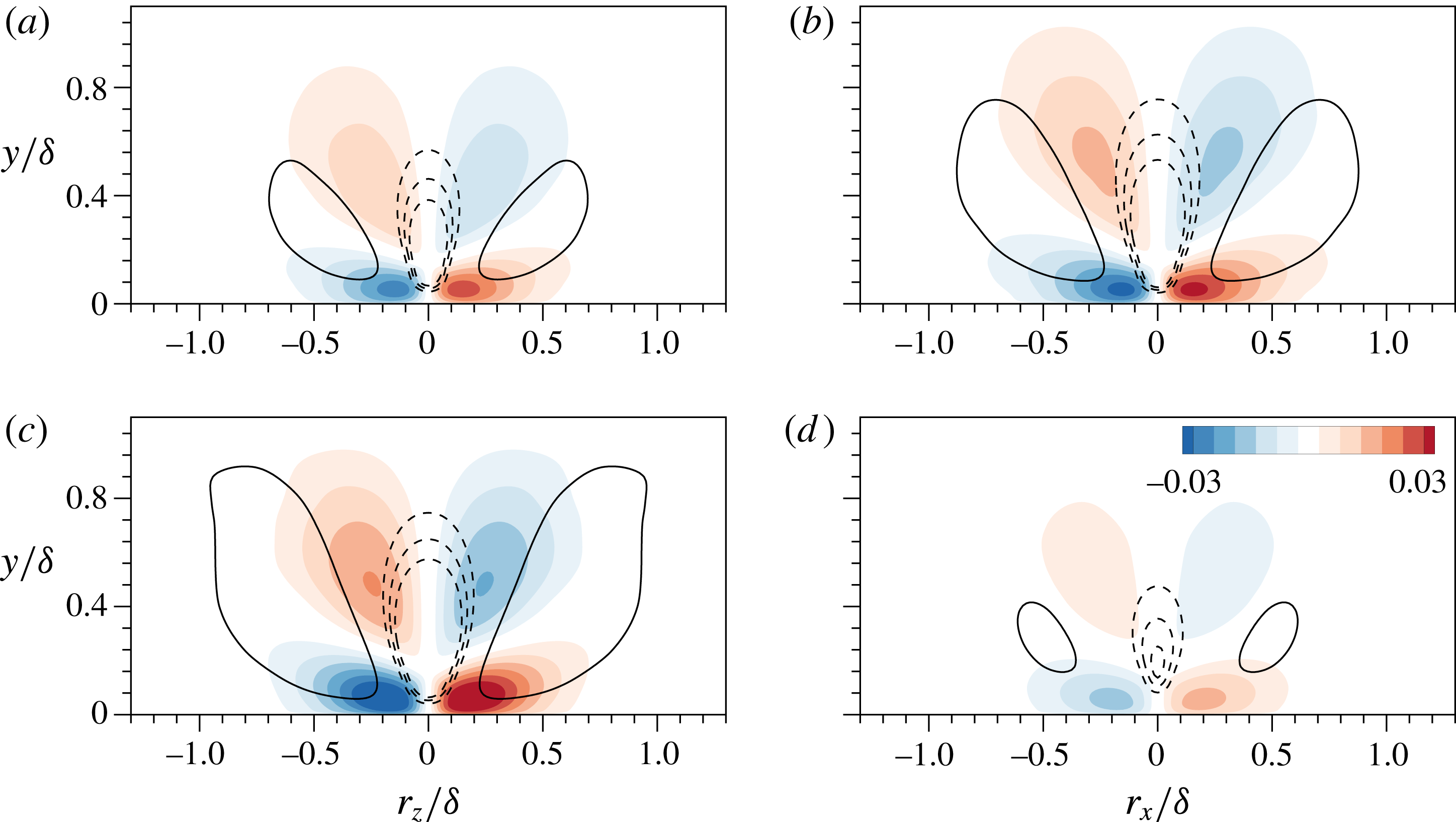
Conditional correlations (
 $R[u_{I},w]$
) in the
 $y$
–
 $z$
plane (
 $r_{x}/{\it\delta}=0$
): (a) nLSM (
 $u_{1}$
); (b) nVLSM (
 $u_{2}$
); (c) pLSM (
 $u_{3}$
); and (d) pVLSM (
 $u_{4}$
). The filled contours are
 $R[u_{I},w]=\pm$
(0.005 : 0.005 : 0.03). The inserted line contours represent
 $R[u_{I},v]$
varied from
 $-$
0.015 to
 $-$
0.025 with an interval of 0.005 (dashed) and
 $R[u_{I},v]=0.006$
(solid).

To investigate the cross-correlation
 $R[u_{I},w]$
in further detail, a cross-section at
 $r_{x}/{\it\delta}=0$
is shown in figure 7. As illustrated by the filled contours, the attached pairs have larger correlations close to the wall and their peaks occur at
 $y^{+}=42$
even though the reference position of the events is located at
 $y/{\it\delta}=0.15$
. Compared to the negative values of
 $R[u_{I},v]$
(dashed lines), the spanwise velocity fluctuations penetrate more deeply towards the wall, which reflects that the footprints of outer large-scale structures are more directly related to near-wall spanwise velocity fluctuations – a result that is consistent with the amplitude modulation of
 $w$
recently reported by Talluru et al. (Reference Talluru, Baidya, Hutchins and Marusic2014). The spanwise locations of the peaks are
 $r_{z}/{\it\delta}=\pm 0.13$
and
 $\pm 0.18$
for the negative- and positive-
 $u$
events, respectively. In other words, the peak distance is wider for the positive-
 $u$
events due to the dispersive motions in the spanwise direction, indicating that the outer large-scale positive
 $u$
could affect near-wall
 $w$
over a larger spanwise extent. Additionally, the contours of
 $R[u_{I},u]$
for negative
 $u$
are gradually narrower under the reference position whereas those for positive
 $u$
are relatively wider in figure 5(a,b). This difference in the shape is due to the opposite direction of spanwise motions in the vicinity of the wall; the congregative motions for negative-
 $u$
and dispersive for positive-
 $u$
footprints.
The line contours of
 $R[u_{I},v]$
which represent the wall-normal fluctuations (
 $v$
) associated with specific
 $u$
events are displayed in figure 7. Around the reference point, the correlations are negative, which is characteristic of Q2 ejections (
 $u<0$
and
 $v>0$
) for the outward motions and Q4 sweeps (
 $u>0$
and
 $v<0$
) for the inward motions (Wallace, Eckelmann & Brodkey Reference Wallace, Eckelmann and Brodkey1972). In particular, nVLSMs and pLSMs are most strongly correlated to the surrounding wall-normal fluctuations,
 $R[u_{2},v]$
and
 $R[u_{3},v]$
. The Reynolds shear stress associated with the ejection and sweep events is therefore dominated by nVLSMs and pLSMs in the log layer. By comparing
 $R[u_{I},v]$
with
 $R[u_{I},w]$
, a pair of large-scale circulations is observed on both sides of the ejection (negative-
 $u$
condition) and sweep (positive-
 $u$
condition). The association between low-speed, large-scale structures and a pair of counter-rotating roll modes was reported in previous studies (e.g. Hutchins & Marusic Reference Hutchins and Marusic2007b
; Chung & McKeon Reference Chung and McKeon2010; Baltzer et al.
Reference Baltzer, Adrian and Wu2013; Talluru et al.
Reference Talluru, Baidya, Hutchins and Marusic2014). Those works mentioned that large-scale circulations have an important influence on the near-wall fluctuations. These opposite wall-normal motions of ejections (
 $v>0$
) and sweeps (
 $v<0$
) each induce opposite spanwise near-wall movements, which can be described as congregative and dispersive, respectively. This highlights an important difference in inner–outer interactions involving large-scale low- versus high-speed events. In addition, the maximum correlation values for nLSM (
 $R[u_{1},w]$
) and nVLSM (
 $R[u_{2},w]$
) are 0.034 and 0.048, respectively, which suggests that the strong congregative motions reside under the nVLSM. In common with
 $R[u_{I},u]$
, the pLSM has the greater maximum value (0.05) relative to the pVLSM (0.025). Hence, the nVLSM and pLSM are the dominant structures that have an effect on the near-wall spanwise velocity fluctuations by inducing strong converging and diverging motions in the near-wall region. In the next section, the influence of the footprints of nVLSM and pLSM are examined by conditionally sampling the near-wall fluctuations that are associated with outer large-scale structures.
3.3. Footprint of outer large-scale structures
The large-scale features with streamwise extent over
 $1{\it\delta}$
are frequently observed near the top of the log layer. Very long motions (
 ${>}3{\it\delta}$
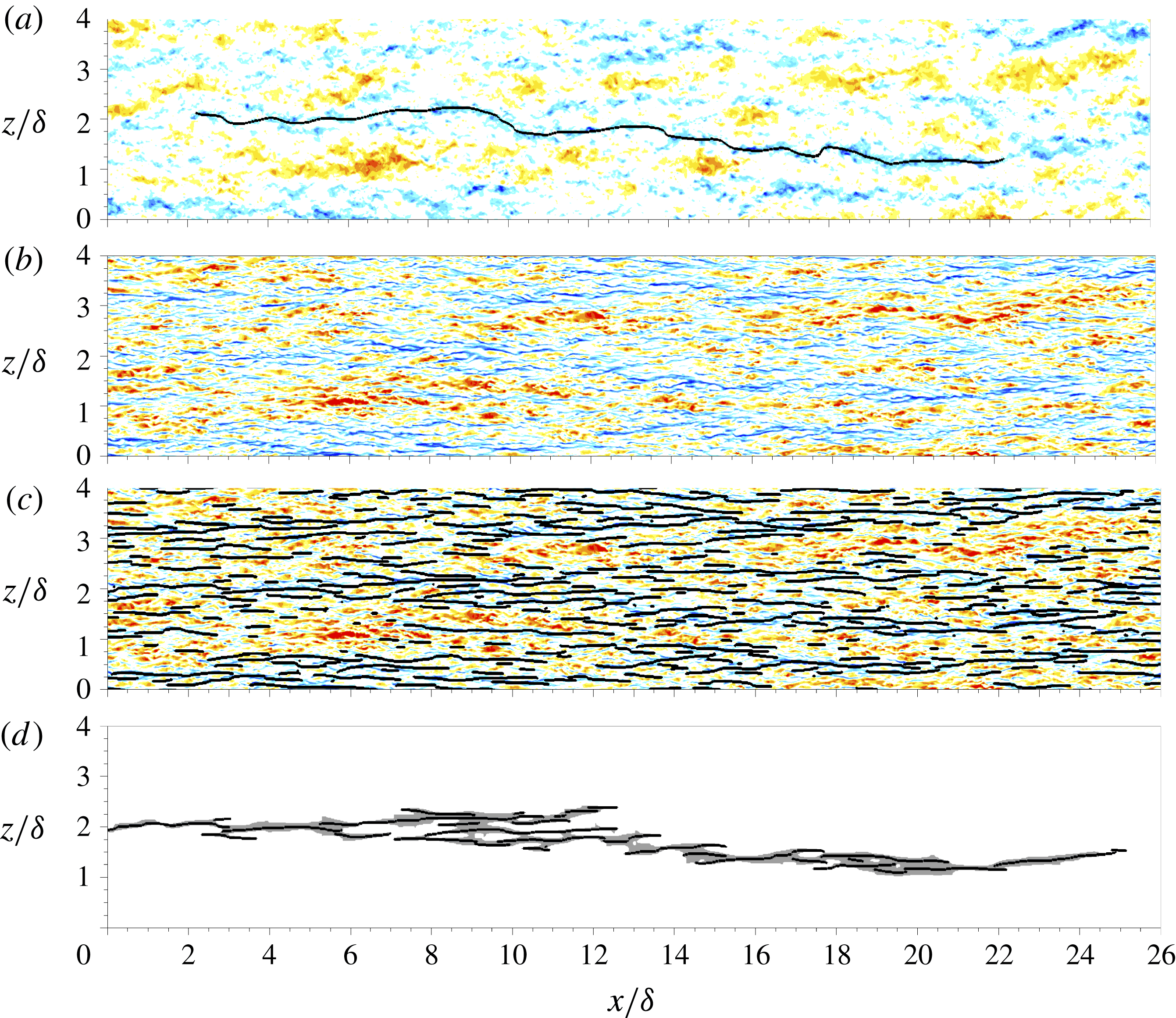
), in particular, are predominantly low-speed events compared to high-speed ones (figure 2). Figure 8(a) shows the streamwise velocity fluctuations in the wall-parallel plane
 $y/{\it\delta}=0.15$
. There are several elongated structures of negative and positive
 $u$
with stripiness over the plane and long low-speed structures are flanked by relatively short high-speed regions. The inserted line represents a conditionally sampled low-speed event with length over
 $21{\it\delta}$
. This structure is visibly similar (typically
 $O(20{\it\delta})$
in length) to that reported by Monty et al. (Reference Monty, Stewart, Williams and Chong2007) and by Hutchins & Marusic (Reference Hutchins and Marusic2007a
), although the present structure is identified using a different technique. Hutchins & Marusic (Reference Hutchins and Marusic2007a
) applied a Gaussian filter in two planes, located in the log and buffer regions of turbulent channel data, and noted the visual similarity between the velocity patterns for both wall-normal positions. They interpreted their observation as the footprints of very long low-speed regions extending down to very near the wall. In figure 8(b) the streamwise velocity fluctuations are plotted at
 $y^{+}=14.5$
. To identify the near-wall regions associated with outer large-scale events (footprints), we conditionally sampled the near-wall
 $CP$
lines (shown in figure 8
c), which are vertically connected to the long
 $CP$
lines (
 $L_{CP}>1{\it\delta}$
) at
 $y/{\it\delta}=0.15$
. The procedure of the footprint identification is summarized below.
-
(1) As noted in § 2.2, the contiguous regions of streamwise velocity fluctuations are identified based on the
 $CP$
in the wall-parallel plane at
$y/{\it\delta}=0.15$
. By measuring the streamwise length of the signed
$CP$
(
$L_{CP}$
), the
$u$
streaks are conditionally sampled in the flow field.
-
(2) To identify the near-wall extent of these long
$u$
motions, the connectivity of the
$CP$
s is traced in the wall-normal direction by comparing adjacent wall-parallel planes (
$j$
and
$j-1$
planes). Neighbouring
$CP$
s connected in the
$j-1$
plane are continuously identified down to the wall. -
(3) Among the near-wall
$CP$
s (figure 8
c), only those that are vertically connected to the reference
$CP$
are conditionally sampled (black lines in figure 8
d). The areas of the near-wall
$CP$
s are determined by measuring their lower and upper bounds similar to figure 1(c). In this manner, we quantify the footprints of outer long
$u$
motions, as marked by the grey shading in figure 8(d).


The detected footprint of nVLSMs (grey area in figure 8
d) is remarkably similar to its outer low-speed event. The collective length of the near-wall
 $CP$
s is over 20
 ${\it\delta}$
. This near-wall arrangement affirms the correlation between near-wall and outer structures, and the view that the near-wall ones are modulated by the outer large scales, consistent with Hutchins & Marusic (Reference Hutchins and Marusic2007b
) and Mathis et al. (Reference Mathis, Hutchins and Marusic2009). To examine this relation further, the near-wall regions which are connected to outer large-scale structures are conditionally sampled from each instantaneous field and their characteristics are analysed.
Instantaneous flow fields in the
 $x$
–
 $z$
plane. The contours show the streamwise velocity fluctuations at (a)
 $y/{\it\delta}=0.15$
and (b–d)
 $y^{+}=14.5$
. In (a), the inserted solid line (
 $CP=-1$
) identifies an nVLSM with 21
 ${\it\delta}$
. The lines in (c) mark
 $CP=-1$
in that wall-parallel plane. In (d), at
 $y^{+}=14.5$
, the solid lines identify the near-wall
 $CP$
that are vertically connected to the line that marks the nVLSM in (a).

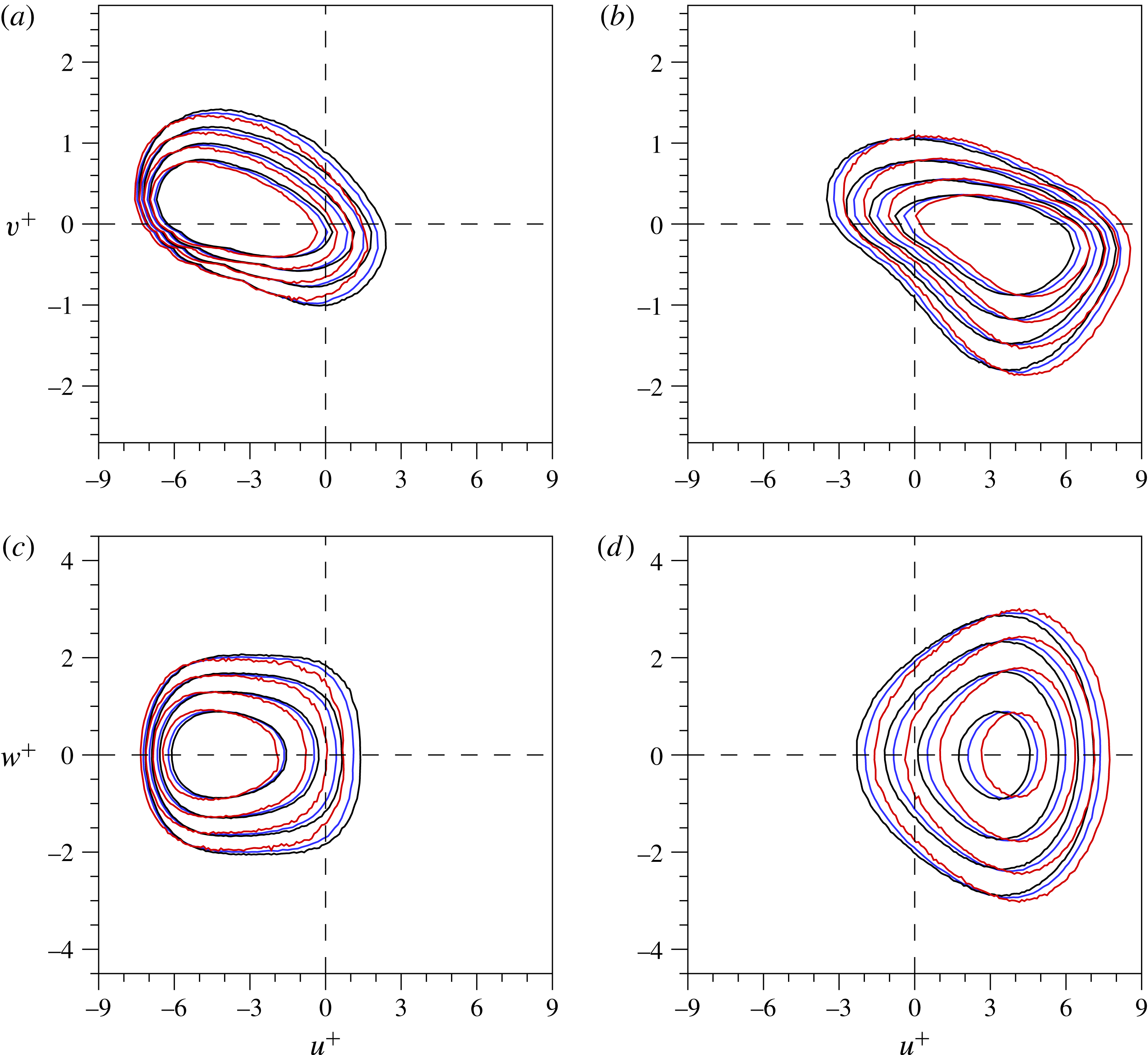
Joint p.d.f.s of (a)
 $u$
–
 $v$
and (b)
 $u$
–
 $w$
at
 $y^{+}=14.5$
. The thinner upper panels show the p.d.f. of
 $u$
and the thinner right panels show the p.d.f. of
 $v$
and
 $w$
. The velocity fluctuations are computed from the detected near-wall
 $CP$
s, which are vertically connected to the outer structures. The blue and red lines represent the velocity fluctuations associated with the footprints of nVLSM (blue) and pLSM (red), respectively. Contour levels are distributed exponentially from 0.005 to 0.05.

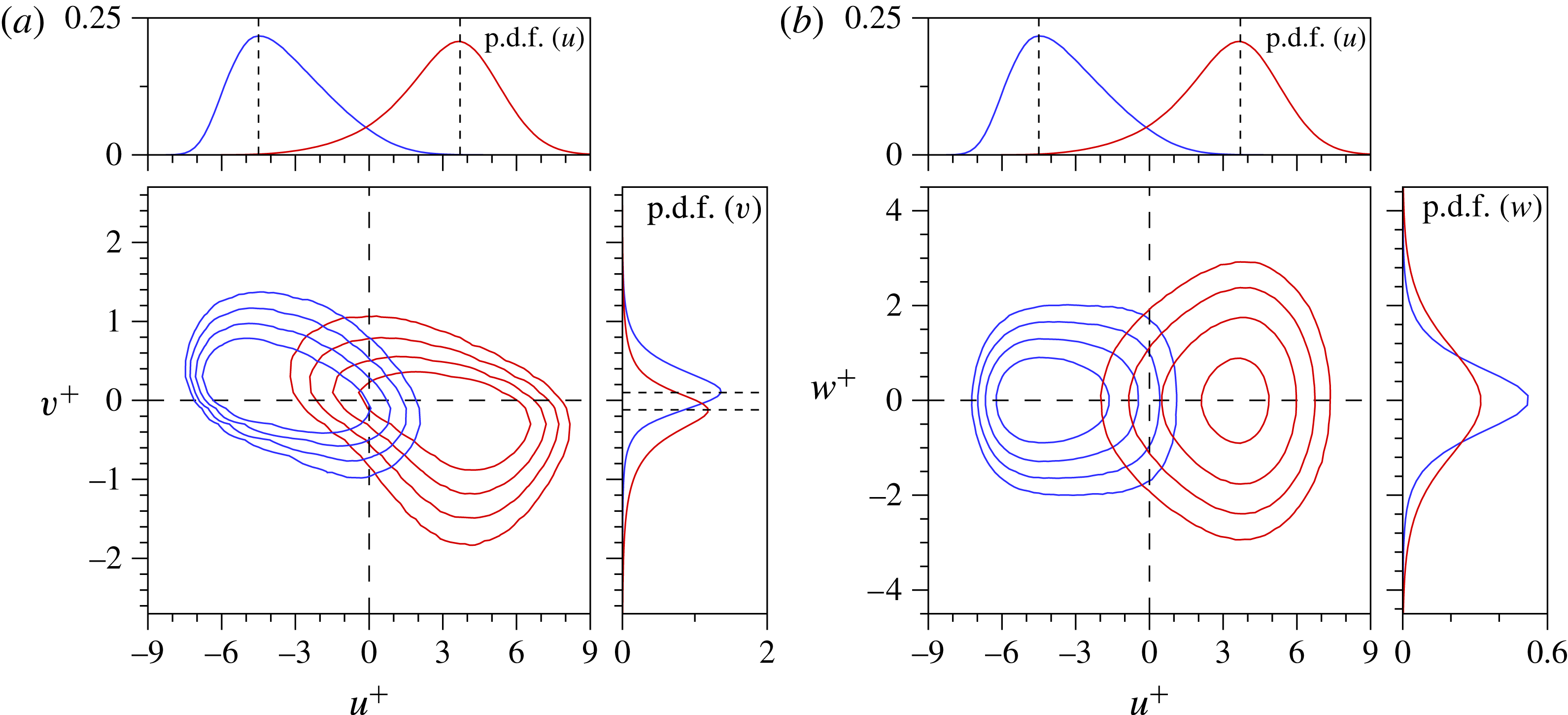
Figure 9 shows the joint probability density function (joint p.d.f.) of (a)
 $u$
–
 $v$
and (b)
 $u$
–
 $w$
at
 $y^{+}=14.5$
. The velocity fluctuations associated with the footprints are identified using the conditionally sampled
 $CP$
s in the near-wall region. Here, the joint p.d.f.s of the nVLSMs (blue) and pLSMs (red) are shown because these are the dominant motions that have an influence on the near-wall region (cf. § 3.2). The joint p.d.f. of
 $u$
–
 $v$
is presented in figure 9(a) and the adjacent upper (right) panel shows the p.d.f. of
 $u$
(
 $v$
). Ejections and sweeps are the principal perturbations on the footprints of nVLSM and pLSM, respectively. However, their distributions are not symmetric with respect to the origin; the contour line of the pLSMs reaches
 $u^{+}=8$
and
 $v^{+}=-1.8$
, whereas that of the nVLSMs reaches
 $u^{+}=7$
and
 $v^{+}=-1.8$
. This difference also appears as a spread in the
 $u$
and
 $v$
p.d.f.s of the pLSMs. The inserted lines mark the peak locations of the p.d.f.s; the characteristic
 $u$
of the footprint of nVLSMs (
 $u^{+}=-4.5$
) is greater than that of the pLSMs (
 $u^{+}=3.7$
). The asymmetry between negative- and positive-
 $u$
events demonstrates that the influence of large-scale structures depends on their sign, consistent with the work by Agostini & Leschziner (Reference Agostini and Leschziner2014). This trend is prominent in the joint p.d.f. of
 $u$
–
 $w$
(figure 9
b). The
 $w$
of pLSMs are widely distributed, while those of nVLSMs are narrowly distributed. The intense
 $w$
are apparent on the footprints of the large-scale positive-
 $u$
event. The wider (narrower) distributions for the pLSMs (nVLSMs) arise due to the spanwise dispersive (congregative) motions shown in figure 7.
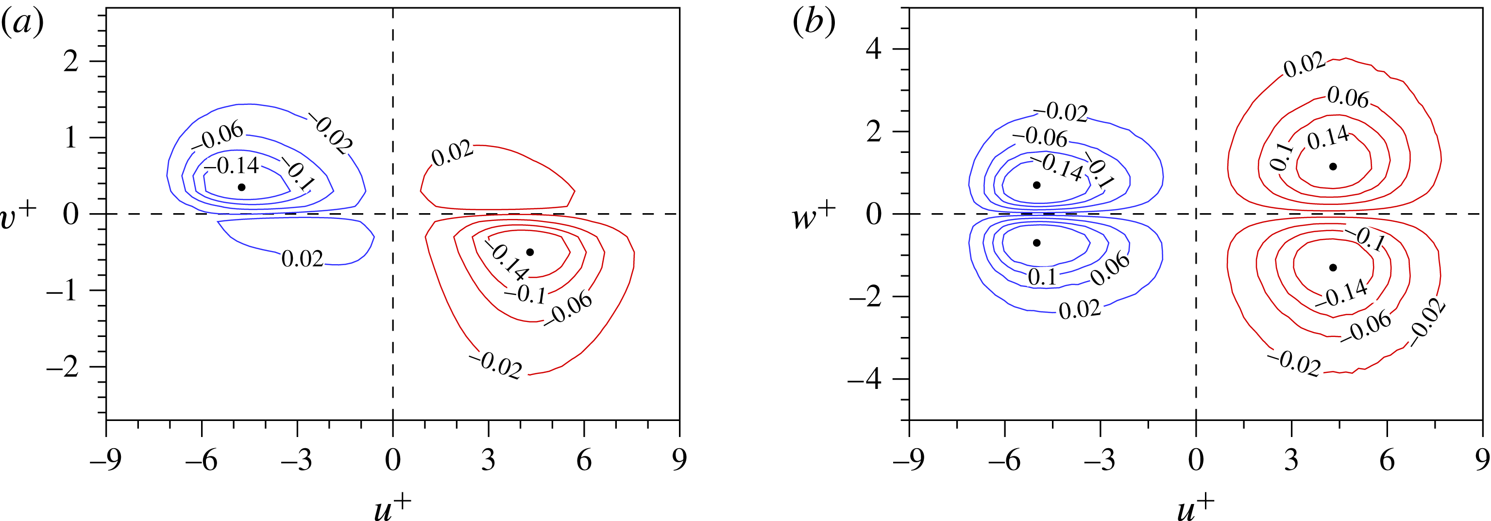
In order to quantify the contributions of the various outer events to the Reynolds shear stress, the weighted joint p.d.f. of
 $u$
–
 $v$
is shown in figure 10(a). The weighted joint p.d.f. is computed by multiplying the joint p.d.f. by
 $uv$
. Note that the results for nVLSM and pLSM are plotted side by side in each panel, with nVLSMs at left and pLSMs at right. The maximum values of the weighted joint p.d.f. are denoted by the black filled circles. For the nVLSMs, the maximum values are
 $u^{+}=-4.75$
and
 $v^{+}=-0.35$
, which are located in the second quadrant. In contrast, the maximum is
 $v^{+}=-0.5$
for the pLSMs. These strong downward motions driven by sweeps of outer positive
 $u$
lead to intense velocity fluctuations even inside the viscous sublayer (not shown here). The difference between the nVLSMs and pLSMs is also apparent in the spanwise velocity fluctuations. Figure 10(b) shows the weighted joint p.d.f. of
 $u$
–
 $w$
, where
 $w$
on the footprints of the pLSMs are clearly greater than those of the nVLSMs. The maximum values of the spanwise component are
 $\pm 1.15$
and
 $\pm 0.7$
for pLSMs and nVLSMs, respectively. The outer large-scale positive-
 $u$
event not only strengthens the near-wall
 $u$
, but also enhances the near-wall
 $w$
. The
 $w$
are appreciably modulated by the pLSMs, even more than
 $u$
and
 $v$
; this is the origin of the highest amplitude modulation coefficient for
 $w$
in the near-wall region, which was reported by Talluru et al. (Reference Talluru, Baidya, Hutchins and Marusic2014). In addition, the discrepancy in the distributions of outer positive- and negative-
 $u$
events in figure 10(b) reflects that the downward motions carried by the positive-
 $u$
structures (sweeps) move the higher-momentum fluid towards the wall where it is spread laterally.
Weighted joint p.d.f.s of (a)
 $u$
–
 $v$
and (b)
 $u$
–
 $w$
at
 $y^{+}=14.5$
. The velocity fluctuations are computed from the detected near-wall
 $CP$
s, which are vertically connected to the outer structures. The blue and red lines represent the velocity fluctuations associated with the footprints of nVLSM (blue) and pLSM (red), respectively. The black circles mark the maximum value of the velocity fluctuations.

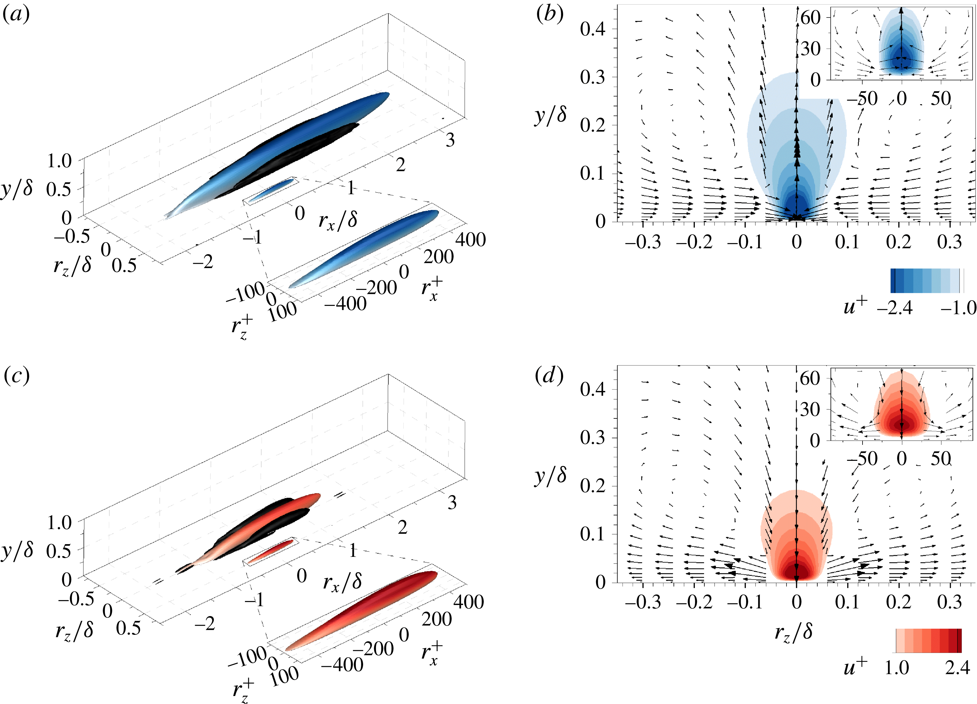
Conditional structures associated with the footprints of nVLSMs (a,b) and pLSMs (c,d) at
 $y^{+}=14.5$
. (a,c) Isosurfaces of the streamwise velocity fluctuations
 $u^{+}|_{FP_{I}}=-1.0$
(blue) and
 $+1.0$
(red). Black isosurfaces are 7 % of the maximum swirling strength. The conditional structures of near-wall streaks that are not connected to outer large scales (
 $u^{+}|_{NWS}$
) are shifted in the spanwise direction by
 $0.5{\it\delta}$
and their magnified views are shown in wall units. (b,d) Conditionally averaged fields in the
 $y$
–
 $z$
plane (
 $r_{x}/{\it\delta}=0$
). Vectors represent the in-plane velocity components.

To examine the flow field around the footprints of nVLSM (
 $u_{I}=2$
) and pLSM (
 $u_{I}=3$
), the conditionally averaged velocity is defined,
 $$\begin{eqnarray}\boldsymbol{u}|_{FP_{I}}(r_{x},y,r_{z})=\langle \boldsymbol{u}(x+r_{x},y,z+r_{z})|CP_{I}(x,y_{ref},z)\rangle ,\end{eqnarray}$$
where
 $CP_{I}$
denotes the streaks that are vertically connected to the outer large scales (
 $u_{I}$
). The reference wall-normal position is
 $y_{ref}^{+}=14.5$
. Figure 11(a,c) illustrates isosurfaces of conditional streamwise velocity fluctuation
 $u|_{FP_{I}}$
. Although the reference wall-normal position was chosen at
 $y_{ref}^{+}=14.5$
, the conditional structures have long streamwise lengths, extending over 4
 ${\it\delta}$
(nVLSM) and 2
 ${\it\delta}$
(pLSM) in the streamwise direction. On the contrary, the conditional averages based on the negative- and positive-
 $u$
streaks that are not connected to the outer large-scale events (
 $u|_{NWS}$
) have streamwise lengths of approximately 1000 wall units and are confined within the near-wall region. Figure 11 clearly shows the scale separation in the near-wall region. In addition, the black isosurface represents the swirling strength educed of the conditionally averaged fields (Zhou et al.
Reference Zhou, Adrian, Balachandar and Kendall1999). Conditional structures of both nVLSMs and pLSMs have a long pair of roll modes on both sides of large negative- and positive-
 $u$
structures. These large-scale circulations are quite different from the smaller rolls associated with the velocity contours of
 $\boldsymbol{u}|_{NWS}$
and which are shown in the zoomed view (insets of figure 11
b,d). The centres of the small rolls are located at
 $y^{+}=40$
and
 $r_{z}^{+}=50$
while those of large-scale circulations are located at
 $y/{\it\delta}=0.2$
and their spanwise width is
 $0.4{\it\delta}$
. Although the large-scale circulations of negative- and positive-
 $u$
structures have similar widths, the maximum swirling strength of the pLSM is 1.3 times greater than that of the nVLSM.
3.4. Formation of long negative-
$u$
structure

The previous section demonstrated that long negative-
 $u$
structures (
 ${>}3{\it\delta}$
) are frequently observed in the log layer compared to positive-
 $u$
ones which prevail in relatively short streamwise extent (
 ${<}3{\it\delta}$
). The analysis also showed that the different flow patterns around
 $u_{I}$
contribute to their distinct near-wall signatures, i.e. congregative versus dispersive. This section focuses on the long negative-
 $u$
structures (
 ${>}3{\it\delta}$
) linked with a pair of large-scale circulations around those structures in order to explain their dominance compared to the positive counterparts. The work by Lee et al. (Reference Lee, Lee, Choi and Sung2014) provides an important background. They found that the low-speed regions with lengths 1–3
 ${\it\delta}$
dominantly undergo merging, and that the merging process was facilitated by the different convection velocities between the upstream and downstream structures. Using conditional spatiotemporal correlations of negative-
 $u$
structures, they showed that the convection velocities of the structures depend on their strength,
 $u$
: weak negative-
 $u$
structures have a relatively higher convection velocity than strong negative-
 $u$
ones. To understand the merging process, it is necessary to explain the cause of the variation in the strength of
 $u$
between the tail and the head of the two structures involved.
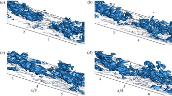
Three-dimensional isosurfaces of negative-
 $u$
structures (
 $u=-0.9u_{th,raw}$
). The time of each instantaneous field is: (a)
 $t_{ref}-3.0{\it\delta}/U_{CL}$
, (b)
 $t_{ref}-1.5{\it\delta}/U_{CL}$
, (c)
 $t_{ref}$
and (d)
 $t_{ref}+1.5{\it\delta}/U_{CL}$
. The isosurfaces are coloured according to their wall-normal distance:
 $y/{\it\delta}<0.1$
(white) and
 $y/{\it\delta}\geqslant 0.1$
(blue).

The merging process of two low-speed structures is captured in figure 12. The blue isosurface represents the outer region,
 $y/{\it\delta}\geqslant 0.1$
. Initially a gap with streamwise length of the order of
 $0.5{\it\delta}$
separates the upstream and downstream structures (figure 12
a). At
 $t=t_{ref}$
, the outer structures start to merge by narrowing the gap, and ultimately form a very long negative-
 $u$
structure. During the merging process, the tail of the downstream structure has a slower convective speed than the head of the upstream one. The slower convection speed of the downstream structure is partly due to the relatively higher magnitude of
 $u$
in that region relative to around the head of the upstream structure. However, the origin of this difference in
 $u$
is unclear and, in light of the correlation between the events in the outer and near-wall flow, a simultaneous investigation of the two regions during the merging process is required. We will demonstrate that this merging process is tightly connected to the spanwise congregative motion under the footprint of large-scale low-speed event.
3.4.1. Time-evolving fields
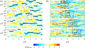
A time series of the velocity perturbation field is shown in figure 13, and captures the merging of two LSMs at
 $y/{\it\delta}=0.15$
. The black lines in figure 13(a) mark the
 $CP$
in the wall-parallel plane, and represent continuous regions of negative
 $u$
. At
 $t_{ref}-1.5{\it\delta}/U_{CL}$
, there are two distinct LSMs, which are marked ‘A’ and ‘B’, and which are not connected to each other; they are separated by a region of positive velocity perturbation. The streamwise lengths of the upstream LSM-A and the downstream LSM-B are of the order of
 $1{-}2{\it\delta}$
, and their spanwise widths are approximately
 $0.4{\it\delta}$
. They advect in the downstream direction with different speeds, with ‘A’ moving faster than ‘B’ even when visualized in the same wall-parallel plane. The downstream structure (LSM-B) is continuously stretched due to the slower advection velocity of its tail relative to its head. On the other hand, LSM-A maintains its length. The gap between the two structures progressively narrows, and they ultimately merge into a single long streak whose streamwise extent is longer than
 $3{\it\delta}$
. The evolution of the near-wall perturbation field during the outer merging process is illustrated in figure 13(b). The black dot identifies the tail position of the LSM-B, and the vertical blue lines are inserted to isolate a region of length
 $1.5{\it\delta}$
beneath the LSM-B. The solid black isocontour marks
 $\hat{u} =0$
. In the marked region, several streaky structures of negative
 $u$
are distributed in the span, separated by a weak perturbation field, and each is initially narrow in width. As the outer LSMs approach one another in the merging process, the near-wall structures congregate within a narrowing window (shown by the blue arrows) and will ultimately form a wide high-amplitude negative-
 $u$
region in the vicinity of the black dot.
Time sequence of instantaneous flow fields in the
 $x$
–
 $z$
plane: (a)
 $y/{\it\delta}=0.15$
and (b)
 $y^{+}=14.5$
. The time of each instantaneous field is marked in each panel. The labels ‘A’ and ‘B’ identify the upstream and downstream LSMs, respectively. In (a), the dashed lines are added to indicate the head and tail positions of the LSMs. In (b), the black circles are the tail positions of LSM-B and the black solid lines indicate
 $\hat{u} =0$
.

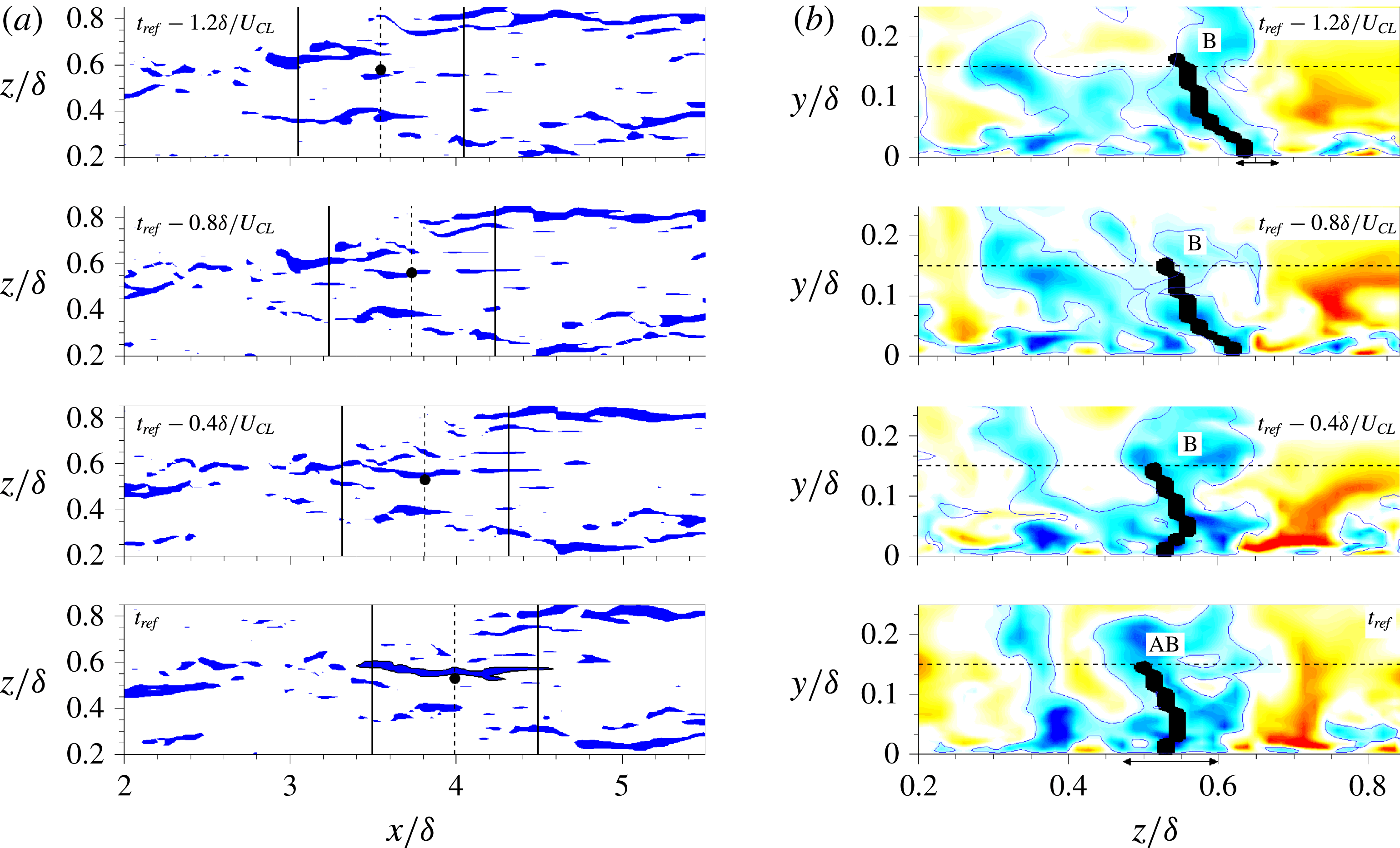
To observe this process in detail, the time sequence of relatively strong near-wall perturbations is shown in figure 14(a). Here, the blue contours illustrate the near-wall streamwise velocity fluctuations lower than
 $-0.2U_{b}$
, which is 1.5 times larger than the local streamwise turbulence intensity. The solid lines are inserted to highlight the behaviour of near-wall structures under the downstream LSM-B; the streamwise distance between the lines is 1000 wall units. Within the bounds of the vertical solid lines, several strong streaky structures are distributed around the dark circle (the tail position of LSM-B in figure 13
a). They gradually congregate under the tail of downstream LSM-B and then form a long streaky structure at later time; the emergent structure is highlighted by the line contour at
 $t=t_{ref}$
(see the supplementary movies available at http://dx.doi.org/10.1017/jfm.2016.3). The formation of concentrated low-speed regions beneath the tail of LSM-B could bring about the retardation of the trailing edge by ejecting the lower streamwise velocity fluid (Toh & Itano Reference Toh and Itano2005).
Time sequence of instantaneous flow fields before the merging event. (a) Streamwise velocity fluctuations (
 $u<-0.2U_{b}$
) in the wall-parallel plane
 $y^{+}=14.5$
. The black circles identify the tail positions of LSM-B. (b) Cross-stream plane at the tail position of downstream LSM-B in figure 13(a). The thick black lines are the cross-stream cut of the characteristic planes (
 $CP$
). The blue line contour indicates
 $u=-0.05U_{b}$
. The dashed horizontal line is at
 $y/{\it\delta}=0.15$
. The contour levels are consistent with figure 13. See also the supplementary movies.

Next, a cross-stream view of the tail of the LSM B is illustrated in figure 14(b). The streamwise position is at the tail of B, which is marked by vertical dashed lines in figure 14(a), and the black line displays a transverse cut of the
 $CP$
which is vertically connected to the outer LSM-B. The solid line extends from the wall since the LSM-B is attached to the wall. At early time, its near-wall spanwise location is
 $z/{\it\delta}=0.64$
and subsequently shifts to
 $z/{\it\delta}=0.53$
later in time. The height of the solid line is largely unchanged, and its terminus away from the wall is insignificantly displaced. Only its origin in the near-wall region is shifted appreciably in the span as the two LSMs A and B merge. As a result, it becomes a relatively straight line through the concentrative movement of the near-wall region under the tail of LSM-B. To highlight the variation in the spanwise size of the structure, the blue line (
 $u=-0.05U_{b}$
) is inserted in the figure. At
 $t_{ref}-1.2{\it\delta}/U_{CL}$
, the near-wall velocity perturbation in the vicinity of the black line switches sign within
 $100{\it\nu}/u_{{\it\tau}}$
in the spanwise direction. Later in time, as the outer structures merge, the width of the near-wall negative-
 $u$
region around the root of the solid line increases significantly. At
 $t=t_{ref}$
, the width becomes
 $0.15{\it\delta}$
, which is greater than the characteristic spanwise width of near-wall structures, through the spanwise merging of surrounding negative
 $u$
that were initially separated by positive
 $u$
.
The instantaneous realizations invoked in the above discussion suggest the possibility of a coupling between the dynamics of a large-scale structure (which induces a congregative motion) and near-wall structures during the merging of outer low-speed streaks. The near-wall negative
 $u$
gradually converge under the outer low-speed region. The driving force behind this congregative motion is the outer large-scale circulations revealed in the conditional correlations in the previous section. The agglomerated negative
 $u$
can lead to the much lower
 $u$
around the tail of the downstream structure if ejected into the outer region. This locally different magnitude of
 $u$
induces the different convection speed of the structure and causes the merging of low-speed streaks. In the remaining sections, conditionally averaged fields are examined in order to provide a statistical account of this merging process and the formation of very-long negative-
 $u$
regions in the log layer.
3.4.2. Streamwise organization of conditional structures
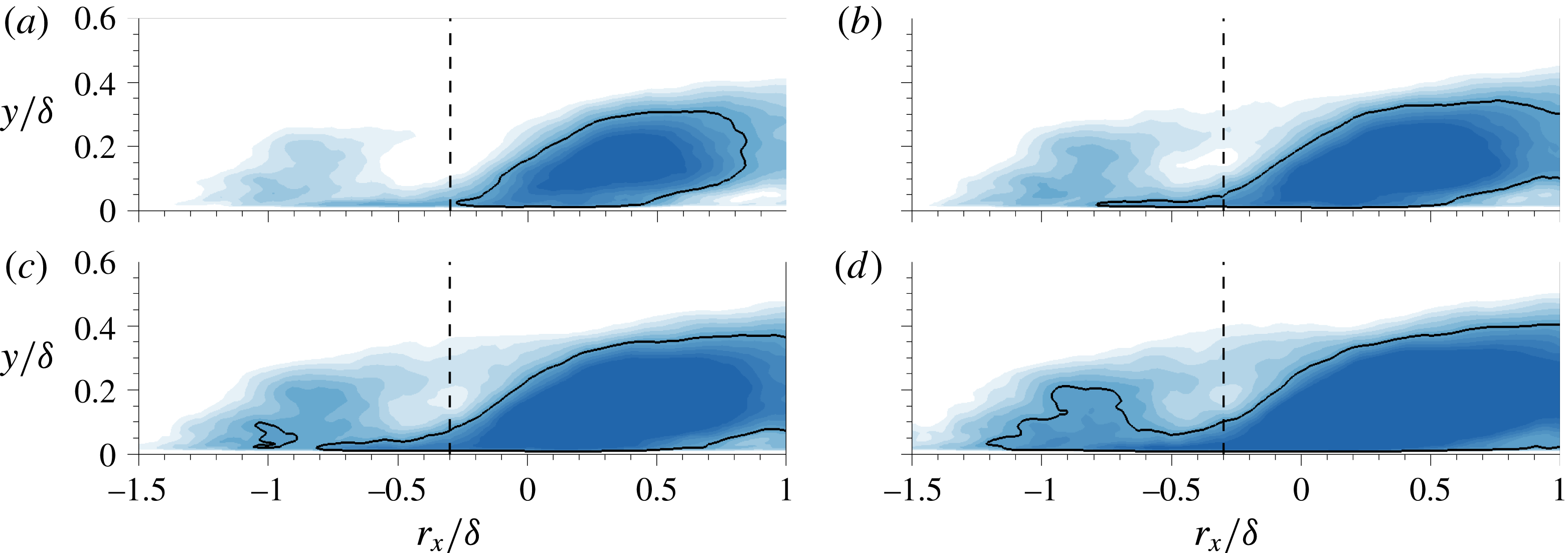
Time sequence of the conditionally averaged velocity fields,
 $u^{+}|_{m}$
, in the
 $x$
–
 $y$
plane (
 $r_{z}/{\it\delta}=0$
): (a)
 $t_{ref}-0.8{\it\delta}/U_{CL}$
, (b)
 $t_{ref}-0.6{\it\delta}/U_{CL}$
, (c)
 $t_{ref}-0.4{\it\delta}/U_{CL}$
and (d)
 $t_{ref}-0.2{\it\delta}/U_{CL}$
. The filled contours range from
 $-0.76$
to
 $-1.2$
with an increment of
 $0.04$
. The line isocountour is
 $u^{+}|_{m}=-1$
.

The formation of very long negative-
 $u$
regions (
 ${\geqslant}3{\it\delta}$
) via the merging process was conditionally sampled from the DNS time series. This enables computation of the averaged flow field associated with merging from the raw velocity fluctuations. The conditionally averaged velocity field is defined as
 $$\begin{eqnarray}\boldsymbol{u}|_{m}(r_{x},y,r_{z};r_{t})=\langle \boldsymbol{u}(x+r_{x},y,z+r_{z};,t-r_{t})|CP^{DT}(x,y_{ref},z;t_{ref})\rangle ,\end{eqnarray}$$
where the superscript
 $DT$
refers to the reference point being the tail position of the downstream structure. The reference position for the conditional averaging is
 $y/{\it\delta}=0.15$
(
 $y^{+}=101$
), and time is measured relative to a reference time,
 $t_{ref}$
, where merging takes place.
A time sequence of conditionally averaged velocity fields,
 $u^{+}|_{m}$
, is shown in figure 15. Although the reference location for the conditional average is at the tail of an outer LSM, another velocity structure of the order of
 $1{\it\delta}$
in length is predicted upstream of the reference position (see figure 15
a). At early time, the two outer structures are separated, but their relative distance decreases in time up to the merging event. The solid contour marks a relatively strong negative-
 $u$
region which is initially restricted to the downstream structure but is gradually enlarged to include the upstream structure. At
 $t_{ref}-0.8{\it\delta}/U_{CL}$
, the most upstream position of the isocontour line represents the tail of the downstream structure,
 $r_{x}/{\it\delta}=-0.3$
. As time evolves, the isocontour line extends in the upstream direction although the velocity structure convects downstream. The streamwise velocity fluctuation intensifies pronouncedly around
 $r_{x}/{\it\delta}\approx -0.3$
, which is near the tail of the downstream structure:
 $u(r_{x}=-0.3,y^{+}=14.5,r_{z}=0)=-1.22$
in figure 15(d), which is 1.3 times enhancement compared to
 $u$
in figure 15(a). The conditionally averaged velocity fields therefore demonstrate a link between the merging of outer structures and intensifying near-wall disturbances. In the instantaneous fields (figure 14
a), the negative-
 $u$
regions under the tail of the downstream LSM progressively intensify prior to merging. The same trends are evident in the conditionally averaged velocity, where the streamwise fluctuations in the near-wall region significantly intensify near the tail of the downstream structure and lead to a slower local convection speed.
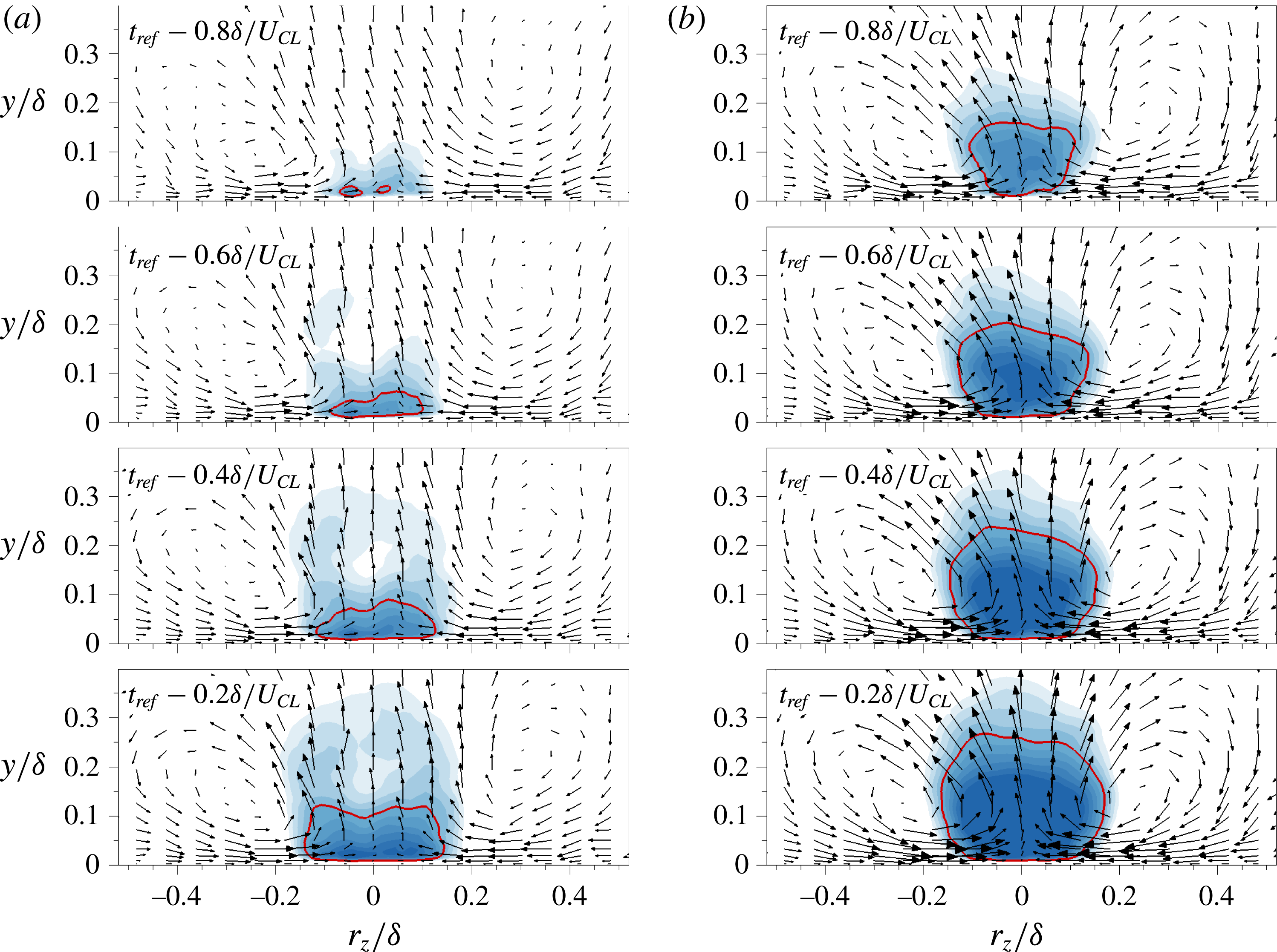
Time sequence of the conditionally averaged velocity fields,
 $u^{+}|_{m}$
, in the
 $y$
–
 $z$
plane for (a)
 $r_{x}/{\it\delta}=-0.3$
and (b)
 $r_{x}/{\it\delta}=0$
. Filled contours range from
 $-0.8$
to
 $-1.25$
with an increment of 0.05, and vectors represent the in-plane velocity components. The red isocontour is
 $u^{+}|_{m}=-1$
.

3.4.3. Near-wall structures and large-scale circulation
The
 $x$
–
 $y$
planes of conditionally averaged fields (
 $u^{+}|_{m}$
) demonstrated that an intense near-wall perturbation is generated at the tail of the downstream structure that partakes in the merging event. Here the focus is placed on the outer roll-cell motion, which is the driving force that leads to this strong near-wall perturbation. Figure 16 shows the time evolution of the near-wall disturbances in the
 $y$
–
 $z$
plane. The vectors are the conditionally averaged in-plane velocities, and the contours show the streamwise velocity perturbation. In figure 16(a), the reference location for conditional averaging is
 $r_{x}/{\it\delta}=-0.3$
, which is marked by vertical dashed lines in figure 15. This position is the most upstream end of the strong negative disturbance
 $(u^{+}|_{m}=-1.0)$
associated with the downstream structure at
 $t_{ref}-0.8{\it\delta}U_{CL}$
. The solid line shows the isocontour level
 $u^{+}|_{m}=-1.0$
in order to mark relatively strong streamwise perturbations, similar to figure 15. At early time, the wall-normal extent of the lowest contour level,
 $u^{+}|_{m}=-0.8$
, is confined within
 $y/{\it\delta}\leqslant 0.1$
. Moreover, there is a pair of large-scale circulations without a strong low-speed event – a notable feature that should be contrasted to previous work on the conditional averages where rolls and low-speed structures coexist (e.g. Hutchins & Marusic Reference Hutchins and Marusic2007b
; Chung & McKeon Reference Chung and McKeon2010; Baltzer et al.
Reference Baltzer, Adrian and Wu2013; Talluru et al.
Reference Talluru, Baidya, Hutchins and Marusic2014). In those studies, both the diameter and the wall-normal location of the core of the large-scale rolls increase downstream. They are therefore inclined relative to the wall at a similar angle as low-speed structures (Talluru et al.
Reference Talluru, Baidya, Hutchins and Marusic2014). In contrast, the cores of the present large-scale circulations observed during the merging process are located at
 $y/{\it\delta}\approx 0.2$
and are not accompanied by a large-scale low-speed event. Close to the wall, the roll modes induce the near-wall congregative motion. As time evolves, the flow response to these large-scale rolls is observed in the form of an amplifying negative-
 $u$
perturbation. Based on the contour level,
 $u^{+}|_{m}=-1.0$
, the width of the
 $u$
response varies from 0.005 to 0.35. Therefore, there is a rapid growth and intensification of the negative-
 $u$
field via the congregative motion induced by the large-scale circulation. In terms of the wall-normal extent, the solid contour in figure 16 initially reaches up to
 $y/{\it\delta}=0.032$
(
 $y^{+}=30$
). It subsequently expands and extends beyond
 $y/{\it\delta}=0.3$
, where the outer merging event takes place (see figure 15). Thus, the intense near-wall congregative motion induced by the outer large-scale circulation transforms into strong streamwise velocity fluctuations at the tail of the downstream structure. Because the local convection speed is proportional to the streamwise velocity fluctuations (Lee et al.
Reference Lee, Lee, Choi and Sung2014), the intense near-wall motions reduce the convection velocity of the downstream large-scale structure and, ultimately, lead to the merging event with the upstream structure.
The conditionally averaged velocity field at the reference streamwise location
 $r_{x}/{\it\delta}=0$
is shown in figure 16(b). The negative-
 $u$
structures, flanked on both sides by high-speed regions, have a width
 ${\rm\Delta}z/{\it\delta}\simeq 0.4$
centred on the event location. Here, the centre of the in-plane circulation is at
 $y/{\it\delta}\simeq 0.15$
and
 $r_{z}/{\it\delta}\simeq \pm 0.25$
, which is similar to the swirling patterns in figure 16(a). The scale of negative-
 $u$
structures is enlarged in both the spanwise and the wall-normal directions. Simultaneously the adjoining large-scale circulations intensify and the near-wall vectors, which are parallel to the boundary, show larger spanwise velocity throughout the merging event. In addition, the large-scale circulation shows that the peripheral sweeps are followed by the opposing spanwise motions near the wall that probably enhance the negative
 $u$
beneath the outer structures. The congregative motion and the increase in the negative
 $u$
in the near-wall region thus accompany and facilitate the formation of the very long low-speed structures during the merging event.
4. Summary and conclusions
Conditional sampling of wall-bounded turbulent flows facilitates the study of the dynamics of turbulence structures, and in particular extracting specific events of interest within the flow field. By applying this technique to flow fields from DNS of turbulent channel flow at
 $Re_{{\it\tau}}=930$
, the spatial feature of long streaks associated with LSM and VLSM, and the accompanying near-wall behaviour, were investigated. Although the negative- and positive-
 $u$
regions occupy similar area fractions within the flow field, their characteristics differ when divided into LSM (
 $1{-}3{\it\delta}$
) and VLSM (
 ${>}3{\it\delta}$
). In the log layer, the positive LSM (
 $1{-}3{\it\delta}$
) occupy a larger area fraction than the negative counterpart. On the other hand, the very long positive-
 $u$
regions (
 ${>}3{\it\delta}$
) are less frequent than the negative ones. The area fractions are consistent with positive perturbations being generally shorter and wider than negative-
 $u$
structures. Based on the conditional two-point correlation, both the footprints of the positive- and negative-
 $u$
structures penetrate into the near-wall region. In addition, the magnitude and patterns of the correlations reveal that nVLSM and pLSM are the dominant structures in the log layer and are directly connected to the near-wall region. The footprints associated with positive
 $u$
are relatively wider than their negative counterpart. The different spanwise scale is due to the character of the near-wall perturbation field induced by the roll motions. The large-scale circulation associated with sweeps generates diverging wall jets in the spanwise direction, while the large-scale circulation associated with negative
 $u$
has the form of ejections with near-wall opposing jets. These different spanwise near-wall motions of the positive and negative structures are parallelled by a difference in their contribution to near-wall Reynolds stresses.
The particular near-wall streaks that are connected to outer large-scale structures were conditionally sampled and their characteristics were analysed. The near-wall
 $u$
under the footprints of positive LSMs are enhanced even in the viscous sublayer compared to the negative-
 $u$
case. Also, the spanwise velocity fluctuations (
 $w$
) are significantly modulated by positive-
 $u$
LSMs, even more than
 $u$
and
 $v$
, which indicates that the large-scale positive-
 $u$
events play a material role in the amplitude modulation of the near-wall small scales. The positive-
 $u$
events also influence a relatively wider near-wall region by inducing the dispersive motion. On the other hand, the near-wall congregative motions of negative-
 $u$
footprints contribute to the formation of very long negative-
 $u$
regions (
 ${>}3{\it\delta}$
) in the log layer. The congregation of near-wall streaks beneath the outer counter-rotating rolls generates intense velocity perturbations which are lifted away from the wall towards the outer large-scale structures. This process enhances the spatial coherence of the negative-
 $u$
structures in the log layer. This same process was shown to take place during, and to partake into, the merging of negative large-scale perturbations to form VLSMs. The dynamics of merging of LSMs were examined using conditional averages with the condition being a merging event at
 $y/{\it\delta}=0.15$
. The results confirmed that the intense near-wall regions are a robust feature during the merging process, although further studies are needed in order to determine whether the generation of intense near-wall perturbations can be fully attributed to the congregation of near-wall streaks. Owing to the existence of large-scale circulations, the intense
 $u$
regions are lifted up and evolve into the trailing edge of the downstream LSM. Since the convection velocity is slower around the strong
 $u$
regions, the downstream LSM is retarded and merges with the upstream structure. As such, the formation of very long negative-
 $u$
regions via merging events is directly related to the evolution of intense near-wall perturbations.
Our results demonstrate the different top-down influence of high- and low-speed large-scale structures, i.e. the dispersive and congregative motions associated with their respective outer large-scale circulations. Furthermore, the retardation of the outer low-speed structure was linked to the evolution of intense near-wall streamwise velocity fluctuations as part of a bottom-up process. The inner–outer interactions of negative-
 $u$
structures lead to their locally different convection velocities. We also directly verify the dynamic role of the outer roll cell, which generates the intense near-wall motions, and ultimately facilitates merging of low-speed streaks into the very long low-speed regions that characterize the outer layer.
Histograms of the streamwise lengths (
 $L_{CP}$
) of low- and high-speed streaks when using various velocity thresholds,
 $u_{th,raw}$
. The bin size is
 ${\rm\Delta}L_{CP}=1{\it\delta}$
. (a) The mean number of the streaks per field (
 $\langle N_{CP}\rangle$
) in the wall-parallel plane. (c) The mean area occupied by the structures per field (
 $\langle {\it\Pi}_{CP}\rangle$
) versus their streamwise lengths. (a,c) The flood and line contours represent low- and high-speed streaks, respectively. Difference in (b) mean number and (d) mean area between low- and high-speed regions; negative values indicate larger mean quantity for the high-speed streaks.

Joint p.d.f.s of (a,b)
 $u$
–
 $v$
and (c,d)
 $u$
–
 $w$
at
 $y^{+}=14.5$
: (a,c) nVLSM and (b,d) pLSM. The threshold values are
 $u_{th,raw}=0.05U_{b}$
(black),
 $0.1U_{b}$
(blue) and
 $0.2U_{b}$
(red). Contour levels are distributed exponentially from 0.005 to 0.05.

Acknowledgements
This work was supported by the Creative Research Initiatives (no. 2015-001828) programme of the National Research Foundation and was partially supported by KISTI under the Strategic Supercomputing Support Program.
Supplementary movies
Supplementary movies are available at http://dx.doi.org/10.1017/jfm.2016.3.
Appendix. Effect of the structure-identification threshold
To address the influence of the threshold value adopted in the structure identification, the populations and area fractions of the structures are re-evaluated over a range of thresholds from 0.05 to 0.3. The contour lines in figure 17(a) represent
 $\langle N_{CP}\rangle$
of the streaks as a function of the threshold level. When the magnitude of
 $u_{th,raw}$
is low, new contiguous regions are detected and previously detected regions combine to form longer structures. Thus the total number of the structures and number of those which reach the maximum length increase. However, the general trends do not change qualitatively, and the quantitative change in inappreciable. Regardless of the threshold value, the populations of the structures decrease logarithmically and the negative-
 $u$
regions are longer than their positive counterparts. Figure 17(b) shows the difference in
 $\langle N_{CP}\rangle$
between the negative- and positive-
 $u$
streaks. The darker grey contours indicate a lower
 $\langle N_{CP}\rangle$
for the negative-
 $u$
streaks. The sign of the contours changes around
 $3{\it\delta}$
independently of
 $u_{th,raw}$
. Figure 17(c) shows the mean area
 $\langle {\it\Pi}_{CP}\rangle$
occupied by the streaks as a function of the threshold value. The peak remains between
 $1{\it\delta}$
and
 $3{\it\delta}$
independent of the threshold. The difference between the low- and high-speed regions is plotted in figure 17(d). Since the area fraction of the very long positive-
 $u$
regions (
 ${>}3{\it\delta}$
) drops rapidly compared to the negative ones for all values of
 $u_{th,raw}$
, the sign of the contours changes at
 $L_{CP}=3{\it\delta}$
.
Figure 18 depicts the effect of three values of the threshold,
 $u_{th,raw}=0.05,0.10,0.20U_{b}$
, on the joint p.d.f.s of
 $u$
–
 $v$
and
 $u$
–
 $w$
at
 $y^{+}=14.5$
. The blue line is a reproduction of the results in figure 9. Although in figure 17 the total number of the detected regions depends on the threshold, the joint p.d.f.s collapse well regardless of
 $u_{th,raw}$
. As the threshold value is doubled, the joint p.d.f.s shift very slightly to a higher magnitude of
 $u$
. The shift is insignificant compared to the change in the threshold value because the present detection method extracts the long
 $u$
regions based on the local maxima in the field. The asymmetry between the distributions of positive- and negative-
 $u$
events in figure 9 persists independently of the threshold for the same reason.