1 Introduction
Interest in flight at hypersonic speeds has led to renewed research efforts on laminar boundary layer transition in hypersonic flows. Besides the interest in fundamental mechanisms, the prediction and control of hypersonic boundary layer transition has a practical importance to surface heating, which increases significantly when the boundary layer becomes turbulent.
Turbulence transition on hypersonic lifting bodies is likely to be dominated by a mean cross-flow velocity component that is subject to a cross-flow instability. The first stage of cross-flow instability dominated transition starts with the process of receptivity (Morkovin Reference Morkovin1990a ,Reference Morkovin b ; Saric, Reed & Kerschen Reference Saric, Reed and Kerschen2002; Reshotko Reference Reshotko2008). Based on linear stability theory, travelling cross-flow modes are more amplified than stationary cross-flow modes. However, the stationary modes are highly receptive to surface roughness which can provide higher initial amplitudes that compensate for their lower amplification rate. As a result, except in instances of higher free-stream turbulence levels (Bippes Reference Bippes1999), the stationary modes are the leading mechanism in cross-flow dominated transition. As stationary cross-flow modes grow in amplitude, they form co-rotating vortices. As a result of their approximate alignment with the inviscid streamlines of the baseline flow, the vortices have a strong integrated effect on the boundary layer. As they reach larger amplitudes, they produce a mean flow distortion that includes the formation of an inflected mean velocity profile (Malik, Li & Chang Reference Malik, Li and Chang1994; Malik et al. Reference Malik, Li, Choudhari and Chang1999; Chernoray et al. Reference Chernoray, Dovgal, Kozlov and Loefdahl2005; White & Saric Reference White and Saric2005). The inflectional velocity profile leads to a secondary inviscid instability that generates small-scale velocity fluctuations and eventually turbulence. These stages of development of the cross-flow instability are presented in comprehensive reviews by Reed & Saric (Reference Reed and Saric1989), Wassermann & Kloker (Reference Wassermann and Kloker2002), Saric, Reed & White (Reference Saric, Reed and White2003) and Bonfigli & Kloker (Reference Bonfigli and Kloker2007).
Experimental efforts on hypersonic cross-flow transition have largely focused on generic shapes such as right-circular cones at an angle of attack, and elliptic cones. The conical flow at incidence generates a streamline-normal pressure gradient which, if properly designed, can lead to a mean cross-flow. Recent experiments by Craig & Saric (Reference Craig and Saric2016) on a right-circular cone at an angle of attack at Mach 6 indicated that the growth and development of stationary and travelling cross-flow modes was largely consistent with that observed in low-speed experiments. However following amplitude saturation, the secondary instability development was slower. This difference can ultimately impact transition, and transition control which is almost completely based on low Mach number experiments.
The approach to control cross-flow dominated transition stems from the extreme receptivity of the instability to surface roughness. This feature was exploited by Corke & Knasiak (Reference Corke and Knasiak1998b ) and Corke, Matlis & Othman (Reference Corke, Matlis and Othman2007) to excite selected wavenumbers of cross-flow modes in the boundary layer over a rotating disk, which is a canonical three-dimensional flow that exemplifies the cross-flow instability.
Saric, Ruben & Reibert (Reference Saric, Ruben and Reibert1998) and Radeztsky, Reibert & Saric (Reference Radeztsky, Reibert and Saric1999) exploited this property in their swept wing experiments to excite fixed spanwise wavenumber stationary cross-flow modes using arrays of micron-sized circular distributed roughness elements. They demonstrated that stationary cross-flow modes at the forced spanwise wavenumber exclusively appeared in the boundary layer. Super-harmonic wavenumbers of the forced wavenumber were also possible to appear, however lower wavenumbers were always completely suppressed.
These observations led to the concept of exciting less-amplified stationary cross-flow modes as a means of controlling transition to turbulence in these flows. The key element was that the spanwise wavenumber of the forced mode had to be higher than those of the naturally amplified band. This would guarantee that no disturbance energy would cascade through nonlinear interactions to lower, more-amplified wavenumbers. Saric et al. (Reference Saric, Ruben and Reibert1998) referred to this approach of cross-flow transition control as ‘subcritical forcing’. This was in reference to the band of initially amplified spanwise wavenumbers being the ‘critical’ wavenumbers. Forcing of that amplified band of wavenumbers is then referred to as ‘critical forcing’.
Transition control comes by biasing the natural selection mechanism by raising the initial amplitude of the less-amplified cross-flow mode at the subcritical wavenumber, so that it initially dominates the instability growth process. The growth of the forced mode inhibits the growth of the more-amplified (critical wavenumber) stationary mode by modifying the basic state. Ultimately the forced mode decays and the flow eventually becomes turbulent. However, in swept wing experiments (Saric et al. Reference Saric, Ruben and Reibert1998; Radeztsky et al. Reference Radeztsky, Reibert and Saric1999; Saric & Reed Reference Saric and Reed2002), the approach has been shown to produce a substantial increase in the transition Reynolds number.
A majority of the experiments on cross-flow dominated transition to turbulence have been performed on swept wings at low, subsonic Mach number. In such experiments (Saric et al.
Reference Saric, Ruben and Reibert1998) patterned surface roughness in the form of hemispherical ‘dots’ with a height of
 $50~\unicode[STIX]{x03BC}\text{m}$
, was found to provide an effective transition delay. The effect of distributed roughness on swept wings at supersonic Mach numbers was investigated by Saric & Reed (Reference Saric and Reed2002), Saric, Reed & Banks (Reference Saric, Reed and Banks2004), Semionov, Kosinov & Levchenko (Reference Semionov, Kosinov, Levchenko and Govindarajan2006) and Semionov & Kosinov (Reference Semionov and Kosinov2007).
There have been a number of cross-flow transition experiments at supersonic Mach numbers. These have primarily been on right-circular cones at angles of attack. These include experiments by King (Reference King1992) at Mach 3.5, and by Wolf & Laub (Reference Wolf and Laub1997) at Mach 1.6. Both of these studies were concerned with correlating transition data between wind tunnel and free-flight experiments. However, King (Reference King1992) was the first to mention the cross-flow instability as a transition mechanism.
In general, the cross-flow instability growth rate is a maximum where the cross-flow Reynolds number is a maximum. The cross-flow Reynolds number is defined as
 $Re_{CF}=V_{max}\unicode[STIX]{x1D6FF}/\unicode[STIX]{x1D708}$
, where
 $V_{max}$
is the maximum cross-flow velocity, normal to the edge inviscid streamline. For a cone at an angle of attack, the cross-flow Reynolds number increases and then decreases from the windward side of the cone to the leeward side. The maximum occurs towards an azimuthal location,
 $\unicode[STIX]{x1D703}\simeq 130^{\circ }$
, where
 $\unicode[STIX]{x1D703}=0^{\circ }$
is the windward most ray on the cone, and
 $\unicode[STIX]{x1D703}=180^{\circ }$
is the leeward most ray.
The recent experiment by Schuele, Corke & Matlis (Reference Schuele, Corke and Matlis2013) was the first to investigate passive and active patterned roughness for transition control on a sharp-tipped right-circular cone at an angle of attack in a supersonic flow. The model consisted of a
 $14^{\circ }$
right-circular cone placed at a
 $4.2^{\circ }$
angle of attack. This gave a ratio of the angle of attack to half-cone angle of
 $\unicode[STIX]{x1D6FC}/\unicode[STIX]{x1D719}_{c}=0.6$
in which the cross-flow instability was the dominant mechanism of transition. The experiments were performed in the Mach 3.5 supersonic low disturbance tunnel (SLDT) at NASA Langley Research Center that is specially designed to minimize acoustic disturbances.
The cone model had removable tips with different discrete roughness configurations. The passive roughness consisted of indentations (dimples) that were evenly spaced around the cone at an axial location that was just upstream of the first linear stability neutral growth branch for cross-flow modes. The active roughness consisted of an azimuthal array of micron-sized plasma actuators that were designed to produce the effect of passive surface bumps. Two roughness azimuthal wavenumbers were examined: one that was in the band of most-amplified stationary cross-flow modes, representing the ‘critical’ roughness condition; and the second being at a 1.5-times higher azimuthal wavenumber that represented the ‘subcritical’ roughness condition intended to suppress transition.
The results showed that the stationary cross-flow modes were receptive to the patterned roughness. Transition front measurements using the Preston tube approach indicated that the transition Reynolds number had increased by 35 % with the subcritical wavenumber roughness compared to a baseline smooth tip, and by 40 % compared to the critical wavenumber roughness.
Given this background, the objective of the present work was to extend the work of Schuele et al. (Reference Schuele, Corke and Matlis2013) into the hypersonic regime to determine if cross-flow dominated turbulent transition could be suppressed with an appropriately patterned discrete roughness. The experiment would be conducted at Mach 6. However contrary to the previous experiment (Schuele et al. Reference Schuele, Corke and Matlis2013), the wind tunnel would be of a conventional (non-quiet) design. Thus, the experiments would examine both the effect of a higher Mach number and the receptivity of the stationary cross-flow modes to the discrete roughness under a higher free-stream disturbance condition. The cone model would be the same as in the previous experiment, but placed at an angle of attack that would allow the same roughness cone tips (azimuthal wavenumber and streamwise location) to be used, therefore allowing a direct comparison to the experiments at the lower Mach number. A pair of high bandwidth total pressure probes mounted on a three-dimensional (3-D) traversing mechanism would be used to document the boundary layer. The probe frequency response would be sufficient to measure pressure fluctuations associated with the travelling cross-flow modes. Azimuthal profiles of the time-averaged total pressure would be used to document the mean flow distortion produced by the stationary cross-flow modes. The axial development of the mean flow would be used to determine the transition locations for the critical and subcritical patterned roughness. Time-resolved pressure fluctuations would be analysed to document the spatial development of the travelling cross-flow modes. In addition, the analysis would seek evidence of a nonlinear interaction between the stationary and travelling cross-flow modes that has been documented in the boundary layer on a rotating disk (Corke & Knasiak Reference Corke and Knasiak1998b ; Corke et al. Reference Corke, Matlis and Othman2007), which is a canonical three-dimensional flow that exemplifies the cross-flow instability.
2 Experimental set-up
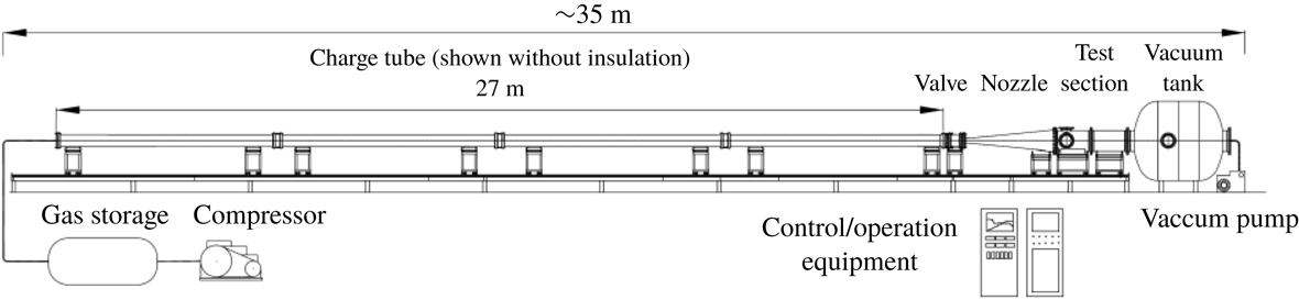
The experiments were conducted in the air force academy (AFA) Mach 6.0 Ludwieg Tube Facility. The facility is based on the design used in the Technical University at Braunschweig, Germany (Estorf, Wolf & Radespiel Reference Estorf, Wolf and Radespiel2004). A schematic of the facility is shown in figure 1. It consists of a 27 m long charge tube that is heated and insulated. The pressurized tube discharges through a converging–diverging nozzle from which a Mach 6 flow exits into an open-jet test section. A fast-acting plunger valve is located just upstream of the nozzle throat. When the valve opens, an unsteady expansion wave travels both upstream and downstream. The upstream moving expansion wave reflects at the end of the charge tube and then travels downstream until it reaches the nozzle. The time for this sets the duration of quasi-steady flow conditions in the nozzle and the hypersonic test section. At the conditions of the experiment needed to produce a unit Reynolds number of
 $10\times 10^{6}~\text{m}^{-1}$
, the run time was approximately 80 ms. Further details of the facility are given by Cummings & McLaughlin (Reference Cummings and McLaughlin2012).
Schematic of U.S. air force academy Mach 6 Ludwieg Tube where the experiments were performed.

The inside diameter of the test section is 0.5 m, and its length is 0.98 m. For optical access, it has three 0.26 m flanged windows, two on opposite sides, and one on top. Measurements in the test section of the sister facility (Estorf et al.
Reference Estorf, Wolf and Radespiel2004) confirmed a non-uniformity of the Pitot pressure in the core flow of approximately
 $\pm$
1.2 %, corresponding to Mach number variations of
 $\pm$
0.6 %. This non-uniformity results from the narrow wake of the upstream fast-acting valve. To avoid this, the cone model was offset from the centreline of the test section.
The model in the experiment was the same as that used by Schuele et al. (Reference Schuele, Corke and Matlis2013). It is a hollow, thin-walled right-circular cone with a half-angle of
 $\unicode[STIX]{x1D719}_{c}=7^{\circ }$
. The total length of the cone is 35.56 cm (14 in.). The first 4.303 cm (1.694 in) (tip) of the cone is removable. The base of the cone mounted to a hollow sting that was connected to a vertical strut. The vertical strut bolted to a base plate that attached to the wind tunnel wall, bridging the joint between the test section and the downstream diffuser section. An angled shim under the base plate was used to orient the cone at the
 $\unicode[STIX]{x1D6FC}=6^{\circ }$
angle of attack. This gave an
 $\unicode[STIX]{x1D6FC}/\unicode[STIX]{x1D719}_{c}=0.86$
, which was in the range of dimensionless angles where King (Reference King1992) had documented stationary cross-flow vortices.
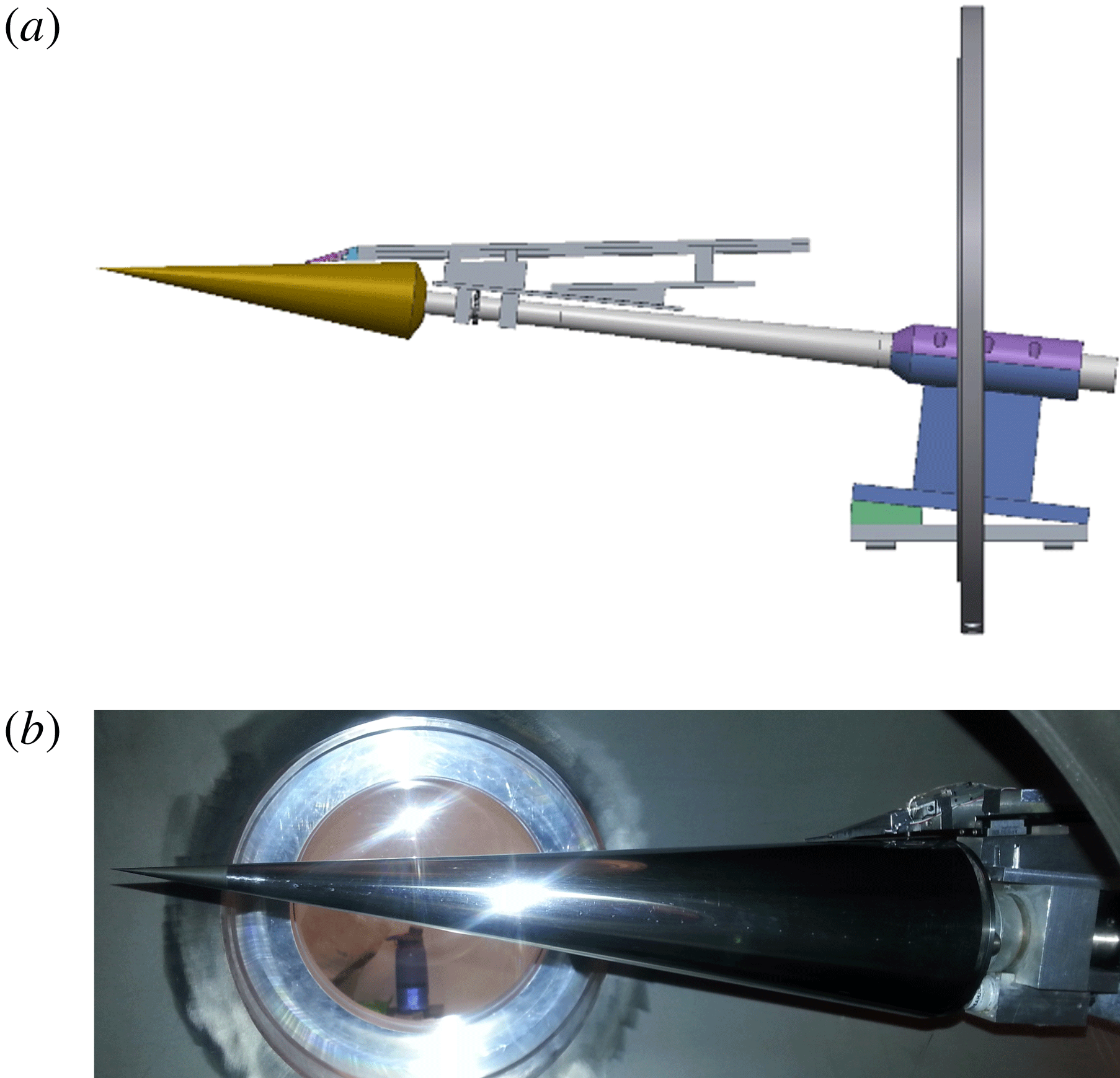
A schematic of the cone, support sting and 3-D traversing mechanism that mounted on the support sting is shown in figure 2(a). A photograph of the cone in the wind tunnel test section is shown in figure 2(b). The wedge-shaped tip of the traversing mechanism that held a pair of high bandwidth total pressure probes is visible near the base of the cone.
Schematic of cone model, sting and traversing mechanism and support base holding the model at a
 $6^{\circ }$
angle of attack (a), and photograph of the cone model inside of the test section.

The traversing mechanism moved a pair of total pressure Pitot probes in the wall-normal, axial and azimuthal directions under computer control. Details of the traversing system are given by Schuele (Reference Schuele2011). The motion resolution in the axial direction was 0.1 mm. The resolution in the azimuthal direction was
 $0.035^{\circ }$
, which was 228 times smaller than the ‘critical’ mode azimuthal wavelength, and 152 times smaller than that of the ‘subcritical’ mode. An optical angle encoder provided feedback to the azimuthal positioning. The resolution in the wall-normal direction was
 $28~\unicode[STIX]{x03BC}\text{m}$
. This utilized miniature linear variable differential transformer to provide motion feedback.
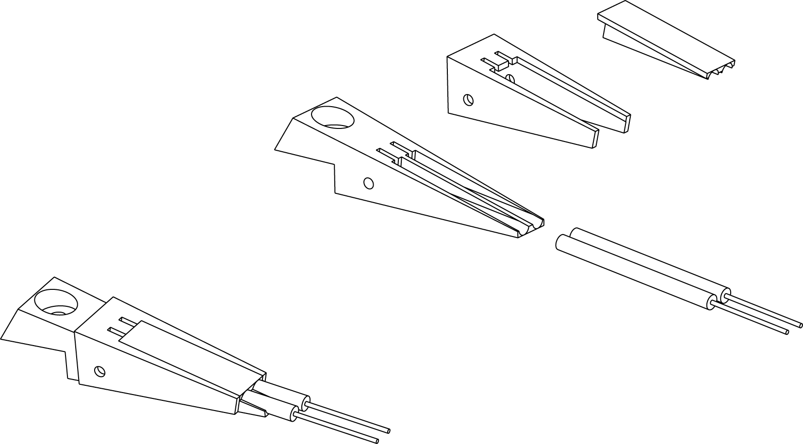
The pair of total pressure Pitot probes utilized Kulite model XCE-062-1.7A (1.7 bar, 25 psi absolute) pressure transducers that were mounted in the wedge tip of the traversing mechanism arm. A schematic of the wedge tip assembly is shown in figure 3. The outside diameter of the Kulite transducers was 1.59 mm. Each transducer was inserted into a circular sleeve whose inside diameter closely matched the outside diameter of the transducer body, and covered the diaphragm end of the pressure transducers. A series of three telescoping hypodermic tubes were then attached to the diaphragm end of the cylindrical sleeve. The hypodermic tubes stepped the outside diameter from 1.72 to 0.81 mm, and gave a final inside diameter of 0.43 mm, which was then the sensing diameter of the Pitot probes. This corresponded to 20 % of the ‘critical’ mode azimuthal wavelength, and 30 % of the ‘subcritical’ mode azimuthal wavelength measured at the middle axial location (12.7 cm) where measurements were performed. The total length of the hypodermic tube assembly was 12.5 mm, which was the same used by Schuele et al. (Reference Schuele, Corke and Matlis2013).
Schematic drawing showing assembly of dual high bandwidth total pressure probe.

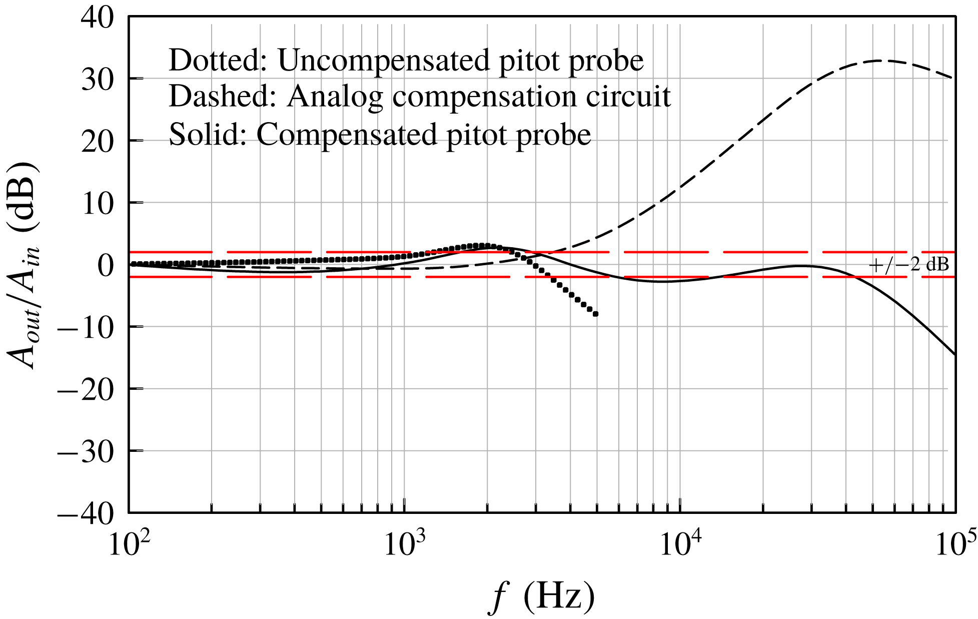
Experiments were performed to determine the frequency response of the Pitot probes. This was accomplished using a sound pressure source with a microphone as a reference. The measured response is shown as the dotted curve in figure 4. This indicates a maximum frequency response, within
 $\pm$
2 dB, of approximately 3.5 kHz. This response was too low to capture the travelling cross-flow modes which based on Li et al. (Reference Li, Choudhari, Chang and White2010) for the conditions of the experiment would be centred about a frequency of 35 kHz. Therefore the output of the Kulite transducers in the Pitot probes was passed through an analogue frequency compensation circuit of our design. The response of the compensation circuit alone is shown by the dashed curve in figure 4. The final response of the frequency compensated Pitot probes is shown by the solid curve in figure 4. The horizontal red dashed lines mark the
 $\pm$
2 dB range. Within this, the compensated Pitot probes have a frequency response of approximately 50 kHz, which is sufficient to capture the travelling cross-flow modes. The time series sampling frequency was 100 kHz.
Frequency response of the uncompensated Pitot probes, the analogue frequency compensation circuit, and the final frequency compensated Pitot probes.

A critical part of the experiment was the design of the roughness tip, specifically the azimuthal wavenumber of the ‘critical’ and ‘subcritical’ roughness, and the axial location for the roughness. The decision drew on experiments at Mach 6 on a
 $14^{\circ }$
right-circular cone at a
 $6^{\circ }$
angle of attack by Swanson & Schneider (Reference Swanson and Schneider2010), and at a close
 $5.6^{\circ }$
angle of attack by Craig & Saric (Reference Craig and Saric2016). Both of these experiments were in quiet tunnels. It also drew on the stability analysis for the conditions of the Swanson & Schneider (Reference Swanson and Schneider2010) experiments that was performed by Li et al. (Reference Li, Choudhari, Chang and White2010). These indicated that the band of most-amplified stationary cross-flow modes was centred near an azimuthal wavenumber of
 $m=45$
. This was then chosen to be the ‘critical’ wavenumber. Based on Saric et al. (Reference Saric, Ruben and Reibert1998), the ‘subcritical’ wavenumber to be excited for control of the stationary cross-flow mode would then be 1.5 times higher or
 $m=68$
.
With regard to the axial location of the roughness, information was taken from the analysis of Li et al. (Reference Li, Choudhari, Chang and White2010) for a unit Reynolds number of
 $10\times 10^{6}~\text{m}^{-1}$
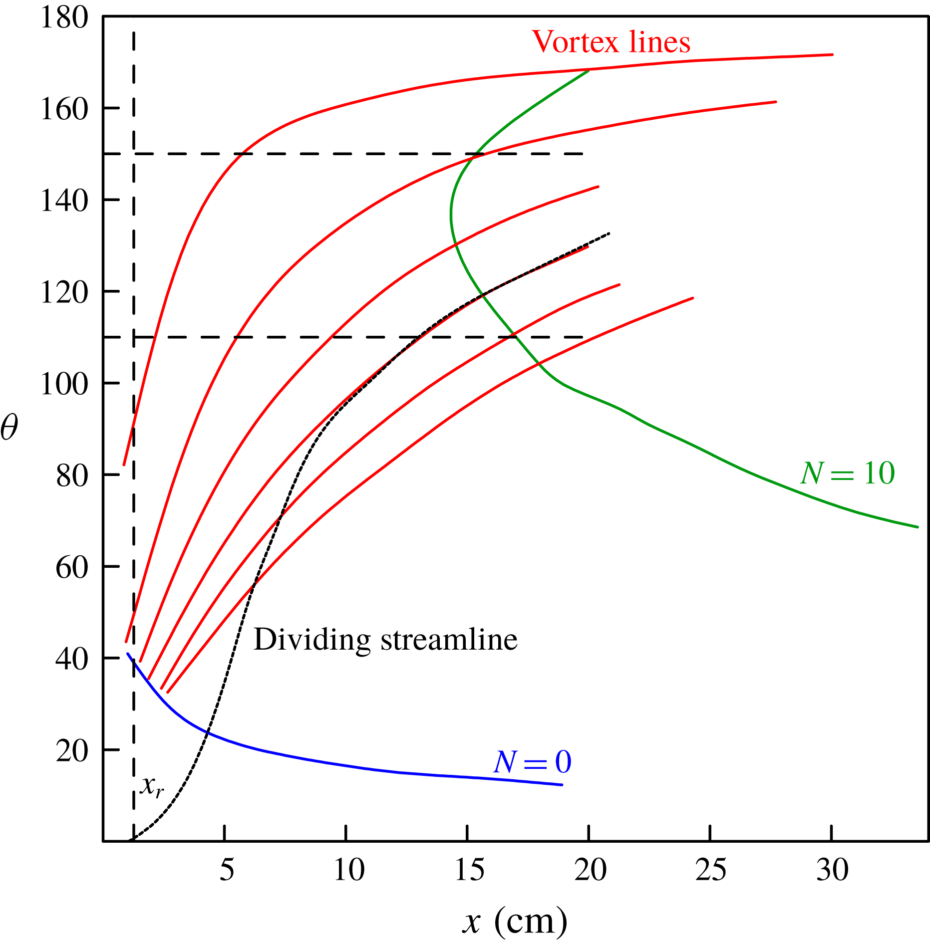
. This is shown in figure 5. The streamwise location of the roughness array is determined by taking into account Branch I (
 $N=0$
) of the linear stability neutral curve for stationary cross-flow modes, as well as the theoretical vortex lines. Placing the roughness array too far upstream of Branch I would allow the controlled disturbances to decay, potentially below the background disturbance level. Placing the roughness too far downstream could allow cross-flow modes excited by random roughness or free-stream disturbances to grow to large enough amplitudes that minimize the effect of the roughness array. An equally important consideration on the placement of the roughness are the theoretical vortex lines, along which the disturbances generated by the roughness convects. To be effective, the axial location of the roughness array needs to intersect with the vortex lines that lead to the region where the linear theory
 $N$
-factor curve reaches furthest upstream on the cone, indicating the most likely region where turbulent transition is expected to occur. For the cone at a
 $6^{\circ }$
angle of attack, this occurs in the azimuthal region on the lee side between
 $110^{\circ }$
and
 $150^{\circ }$
(where
 $0^{\circ }$
is the windward stagnation line). Based on these two factors, the discrete roughness arrays were located
 $x_{r}=1.27~\text{cm}$
from the tip of the cone. This happens to be the same axial location of the roughness as used by Schuele et al. (Reference Schuele, Corke and Matlis2013), although at a different angle of attack and Mach number. As a result, the same roughness tips and design were utilized in the present experiment.
Linear stability and vortex path map used in determining axial location of discrete roughness for cross-flow transition control based on Li et al. (Reference Li, Choudhari, Chang and White2010).

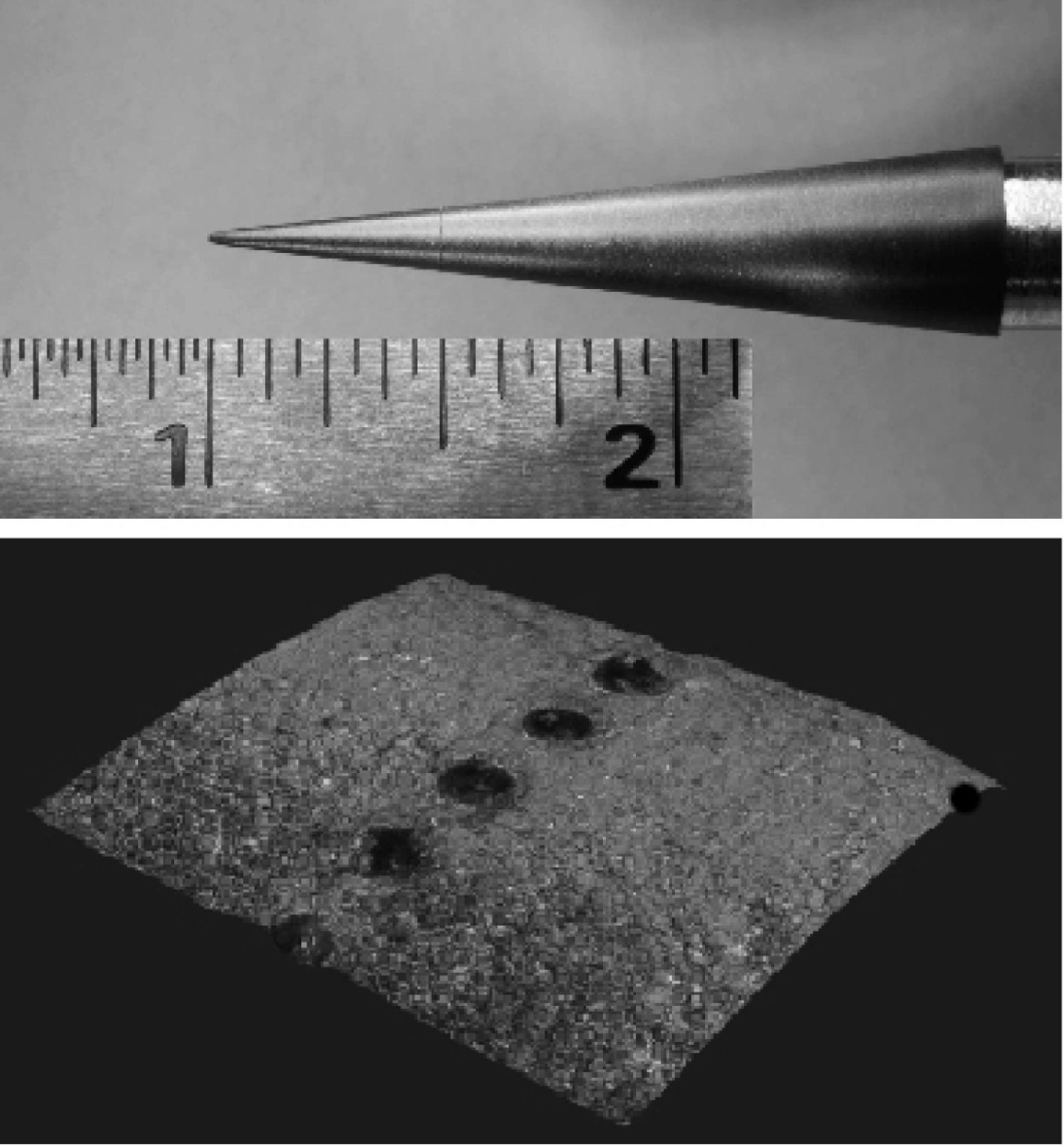
The removable cone tips were machined from Torlon (Polyamide-Imide (PAI)), which is a relatively hard polymer that can be polished. Following Schuele et al. (Reference Schuele, Corke and Matlis2013), the surface roughness patterns consisted of ‘dimples’ that were produced by plunging a conical pin into the surface of the tip. An example of the dimple roughness is shown in figure 6. This corresponds to the
 $m=68$
‘subcritical’ azimuthal wavenumber. The dimple diameter was approximately
 $80~\unicode[STIX]{x03BC}\text{m}$
, and the ratio of the diameter to dimple centreline spacing was
 $d/\unicode[STIX]{x1D706}\simeq 0.6$
. For the
 $m=45$
‘critical’ azimuthal wavenumber, the dimple diameter was approximately
 $145~\unicode[STIX]{x03BC}\text{m}$
, and the ratio
 $d/\unicode[STIX]{x1D706}=0.65$
. In both roughness cases, the spacing between dimples satisfied the discrete roughness criteria (Saric W. S. 2008 Private communication) that
 $d/\unicode[STIX]{x1D706}\geqslant 0.5$
.
The depth of the dimple holes was based on the extent that the conical pin was inserted into the surface to achieve the required dimple diameter. For the larger diameter dimples for the
 $m=45$
‘critical’ azimuthal wavenumber, the depth of the dimple holes was
 $39~\unicode[STIX]{x03BC}\text{m}$
. For the smaller diameter dimples used for the
 $m=68$
‘subcritical’ azimuthal wavenumber, the depth of the dimple holes was proportionately small at
 $21~\unicode[STIX]{x03BC}\text{m}$
. We do not think the dimple depth is a critical parameter. For example, Reibert (Reference Reibert1996) observed that for a fixed (subcritical) roughness spacing of
 $z=12~\text{mm}$
, the total disturbance amplitude grew to a constant saturation amplitude even when the roughness height was varied from 6 to
 $48~\unicode[STIX]{x03BC}\text{m}$
. Although the initial disturbance amplitude increased with larger roughness, the effects downstream relaxed and yielded similar looking mode shapes. Additionally Reibert (Reference Reibert1996) documented that as the roughness height increased from
 $6~\unicode[STIX]{x03BC}\text{m}$
to
 $18~\unicode[STIX]{x03BC}\text{m}$
, in
 $6~\unicode[STIX]{x03BC}\text{m}$
increments obtained by stacking the roughness elements, transition occurred at the same location for all three roughness heights.
Photograph of a removable cone tip with representative ‘dimples’ located at
 $x_{r}=1.27~\text{cm}$
. (0.5 in.) from the tip.

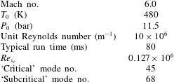
Summary of experimental conditions.

3 Results
These results document the receptivity of the stationary cross-flow mode to the passive patterned roughness with critical and subcritical azimuthal wavenumbers. These controlled stability experiments are the first to be performed at a hypersonic Mach number with free-stream disturbance conditions in which the acoustic disturbances were not minimized through a ‘quiet’ nozzle design. The experimental conditions are summarized in table 1.
3.1 Surface flow visualization
The first objective was to verify that stationary cross-flow were observable under the conditions of the AFA facility. The key issue is that the AFA Ludwieg tube is a conventional design rather than a ‘quiet’ design. There is no previous evidence in the literature of observations of stationary cross-flow modes in conventional (non-quiet) hypersonic wind tunnels. A possible reason is the potential dominance of travelling cross-flow modes, which are more amplified than the stationary modes, and sensitive to free-stream disturbances (Bippes Reference Bippes1999).
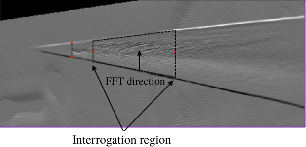
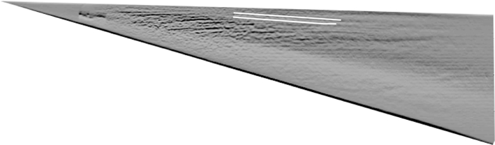
Following Schuele et al. (Reference Schuele, Corke and Matlis2013), the presence of stationary cross-flow modes was first verified using surface oil flow visualization. The approach was to apply to the surface of the cone a mixture of 15 parts 1000 cSt silicon oil, 5 parts Oleic acid and 1 part titanium-dioxide powder. The motion of the oil was recorded during the 80 ms run time of the facility using a high-speed video camera. During the run, the oil pattern would reach a steady pattern that revealed the presence of the stationary cross-flow mode. Image processing was performed on selected frames of the videos. This included Sobol edge detection to highlight the stationary pattern, rotation of the image to account for the angle of attack, mapping of the curved surface onto a flat surface. Figure 7 shows a sample image following this processing. Spatial spectral analysis was then performed in the denoted interrogation region to determine the wavenumbers of features in the oil visualization image.
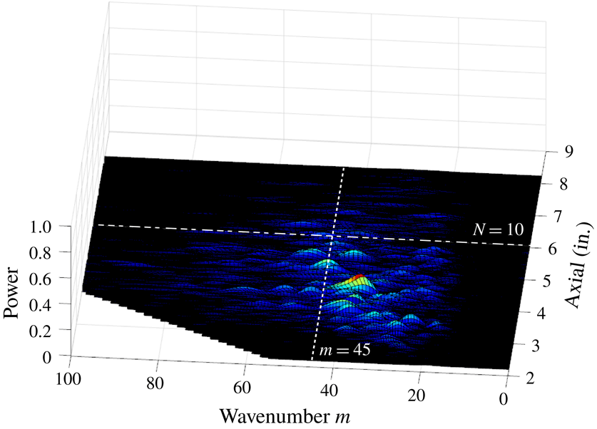
The azimuthal wavenumber distribution for the baseline (smooth tip) flow is shown in figure 8. The dashed line at
 $m=45$
represents the centre of the band of most-amplified stationary cross-flow modes based on Li et al. (Reference Li, Choudhari, Chang and White2010). The dot-dashed line indicates the axial location on the cone where transition would occur based on a linear theory
 $N$
-factor of 10.
Sample processed image of oil flow surface visualization.

Azimuthal wavenumber spectrum axial distribution based on flow visualization for baseline cone (smooth tip) condition.

Figure 8 indicates a broad distribution of energy at wavenumbers that are approximately centred on
 $m=45$
, which is consistent with the linear theory predictions. The energy in this band of wavenumbers diminishes beyond the axial location of the
 $N=10$
line. This indicates that the coherent stationary pattern in the surface visualization is lost beyond this
 $x$
-location, possibly as a result of turbulent transition. Using POD methods in the analysis of swept-wing boundary layer transition Glauser et al. (Reference Glauser, Saric, Chapman and Reibert2014) indicated that the primary mode was still correlated downstream of the transition location. Therefore a more definitive estimate of the transition location will come from the off-wall total pressure measurements presented in the next section.
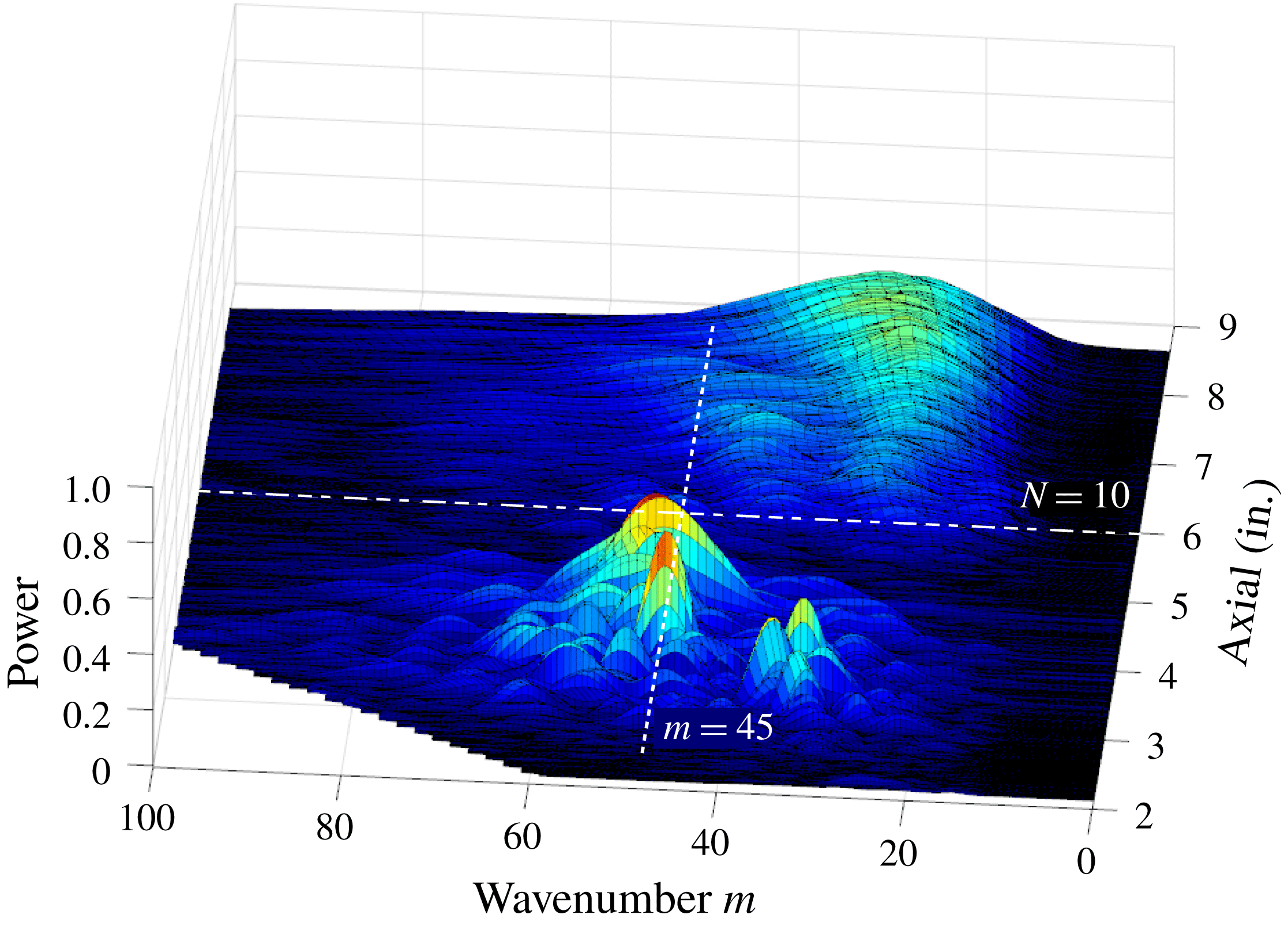
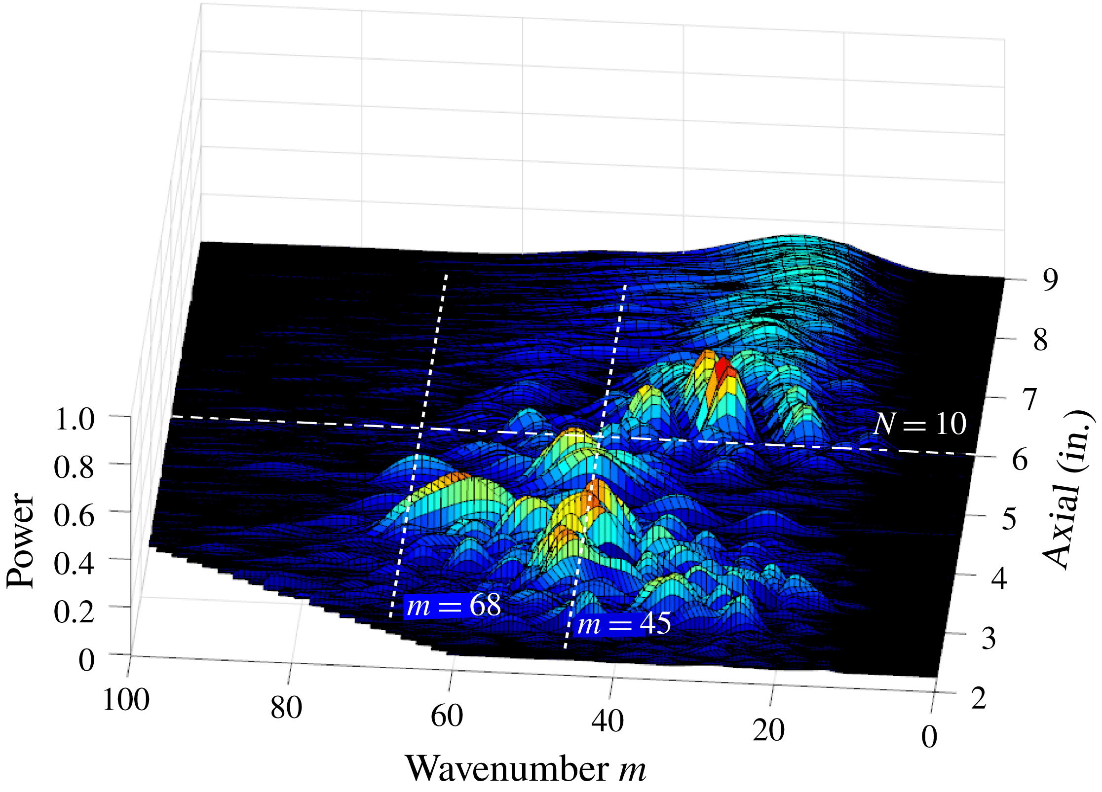
Similar surface flow visualization and image processing was performed for the cases with the ‘critical’ and ‘subcritical’ roughness cone tips. The wavenumber spectra for these are shown in figures 9 and 10, respectively. Note that the amplitude scale on these spectra plots is the same as in figure 8 for the smooth cone tip, to allow a direct comparison.
Azimuthal wavenumber spectra based on flow visualization for cone with ‘critical’ (
 $m=45$
) roughness tip.

Azimuthal wavenumber spectra based on flow visualization for cone with ‘subcritical’ (
 $m=68$
) roughness tip.

In contrast to the smooth tip case, the wavenumber spectra for the ‘critical’ roughness cone tip shows a dominant peak at
 $m=45$
. This indicates that the stationary pattern in the surface visualization was well correlated with the
 $m=45$
roughness wavenumber.
The wavenumber spectrum for the case with the ‘subcritical’ (
 $m=68$
) roughness cone tip reveals a peak around
 $m=68$
that was not previously evident with either the smooth cone tip, or the ‘critical’ roughness tip. In addition, a broad peak near
 $m=45$
is observed. The amplitude of this broad peak is approximately 30 % lower than that with with the ‘critical’ roughness tip, but larger than that with the smooth tip.
These wavenumber spectra of the surface flow visualization offers a first glimpse of the effect that the ‘subcritical’ roughness might have on the transition location. If transition is defined as a loss of coherence of the stationary pattern, then for the ‘critical’ roughness this appears to occur very close to the axial location where the
 $N=10$
line is drawn. In contrast with the ‘subcritical’ roughness, well defined spectral peaks in wavenumber spectra exist well beyond the
 $N=10$
transition line. This might suggest that the transition has been suppressed by the ‘subcritical’ roughness. Further evidence will come from off-wall Pitot probe measurements.
3.2 Pitot probe measurements
As described in § 2, the Pitot probe response was frequency compensated out to 50 kHz, and sampled at 100 kHz. This was important not only to capture a sufficient number of time series points to obtain converged statistics within the short (80 ms) run times, but also to resolve the most-amplified travelling cross-flow modes that were predicted (Li et al. Reference Li, Choudhari, Chang and White2010) to be centred at 35 kHz.
Total pressure time series were sampled at discrete
 $(\unicode[STIX]{x1D703},x)$
locations at a fixed height above the surface of the cone. The data samples at each location represented one run of the facility. In total, there were of the order of 350 runs to generate the data presented in the following figures. For efficiency, the sampled locations were grouped in a range of spatial locations where transition was first expected to occur based on an
 $N$
-factor of 10 that was indicated in figure 5. This corresponded to
 $126^{\circ }\leqslant \unicode[STIX]{x1D703}\leqslant 143^{\circ }$
, and
 $11.43~\text{cm}\leqslant x\leqslant 17.78~\text{cm}$
.
To complement and validate the results from the surface flow visualization, the Pitot probe surveys were used to provide a direct measure of the mean flow distortion produced by the stationary cross-flow modes. This involved averaging the total pressure taken over the duration of a run at each
 $(\unicode[STIX]{x1D703},x)$
location.
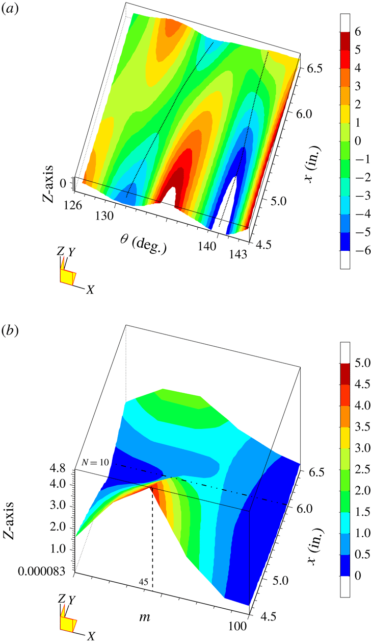
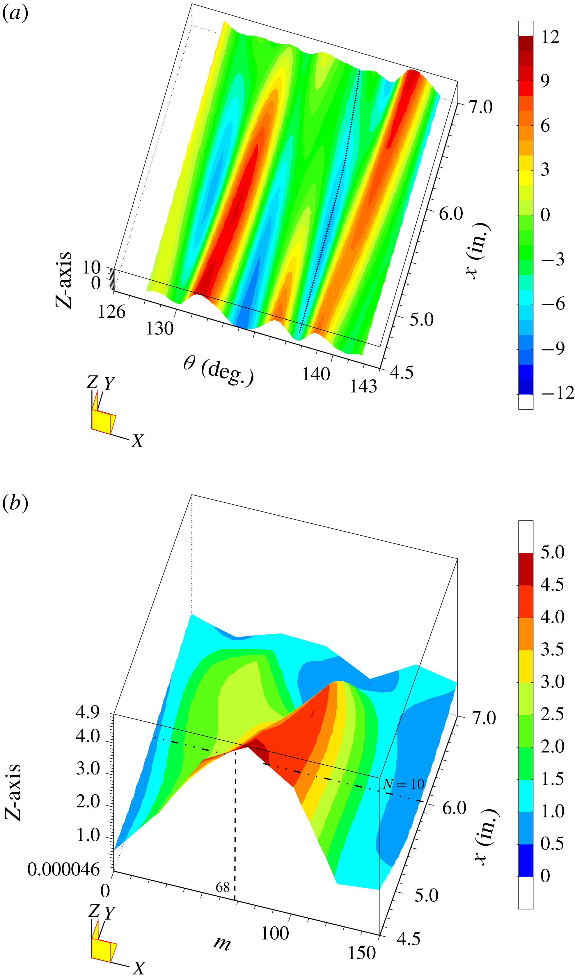
Figure 11(a) shows the azimuthal variation in the time-average total pressure at a fixed height above the cone surface with the ‘critical’ (
 $m=45$
) roughness tip. A consequence of remaining at a fixed height,
 $y$
, above the cone surface is that as the boundary layer thickens in the azimuthal direction along the lee side of the cone, the sensor moves deeper in the boundary layer so that
 $y/\unicode[STIX]{x1D6FF}$
is not constant. In order to better reveal the mean flow distortion produced by the stationary cross-flow modes, this mean trend has been removed. The colour rendering of the total pressure is then presented as the deviation (plus or minus) about the local mean value. This clearly reveals the azimuthal variation in the total pressure that is indicative of the mean flow distortion produced by the stationary cross-flow mode. Note that negative mean-removed pressures correspond to a locally thickened portion of the boundary layer, and positive mean-removed pressures to locally thinned portions. The dotted curves in the figure traces out the
 $x$
-development of two of the azimuthally thickened portions of the boundary layer. This trajectory should correspond to that of two neighbouring stationary cross-flow vortices. As a check, these trajectories have been mapped to the curved coordinate and overlaid on the surface flow visualization image for the same ‘critical’ roughness condition. This is shown in figure 12. The traces are drawn to the same scale as the image and shown in yellow. This shows a good correspondence between the azimuthal measurements of the total pressure and the flow visualization image.
Azimuthal total pressure distributions at a constant height above the surface (a) and corresponding wavenumber spectra (b) for the case with the ‘critical’ (
 $m=45$
) roughness cone tip.

The azimuthal wavenumber of the azimuthal pattern of positive and negative pressure shown in figure 11(a) has an azimuthal wavelength of approximately
 $8^{\circ }$
which coincides with that of the ‘critical’ roughness, namely
 $360^{\circ }/45$
. Evidence of this azimuthal wavenumber is further reinforced by the wavenumber spectra of this total pressure distribution that is shown in figure 11(b). This shows a dominant peak at
 $m=45$
. The energy in the
 $m=45$
mode decays to a minimum near the axial location where the
 $N=10$
factor predicts transition to occur. This agrees well with the wavenumber spectra that was derived from the flow visualization and shown in figure 9.
Overlay (white) of the
 $(\unicode[STIX]{x1D703},x)$
trajectories of the mean flow distortion-thickened boundary layer in figure 11(a) onto a surface visualization image for the same ‘critical’ roughness condition.

The azimuthal variation in the total pressure indicative of the mean flow distortion produced by stationary cross-flow modes with the ‘subcritical’ (
 $m=68$
) roughness is shown in figure 13(a). The contrast with the ‘critical’ roughness case is immediately apparent and reflects the higher azimuthal wavenumber (smaller azimuthal wavelength) that results from the closer spaced discrete roughness at the tip. For reference, the
 $m=68$
mode has an azimuthal wavelength of
 $5.3^{\circ }$
. The wavenumber spectra of the total pressure distribution for this roughness condition is shown in figure 13(b). This shows a dominant peak at
 $m=68$
. Further downstream, the peak appears to shift to higher wavenumbers of the order of 100. This is consistent with Saric et al. (Reference Saric, Ruben and Reibert1998) where subcritical roughness with azimuthal wavenumbers of 1.5-times that of the critical roughness value would not generate subharmonic mode numbers. Similarly Schuele et al. (Reference Schuele, Corke and Matlis2013) observed only higher azimuthal wavenumbers generated by the ‘subcritical’ roughness in their experiment at Mach 3.5.
Azimuthal total pressure distributions at a constant height above the surface (a) and corresponding wavenumber spectra (b) for the case with the ‘subcritical’ (
 $m=68$
) roughness cone tip.

The dominant peak in the wavenumber spectra with the subcritical roughness extends well downstream of the
 $N=10$
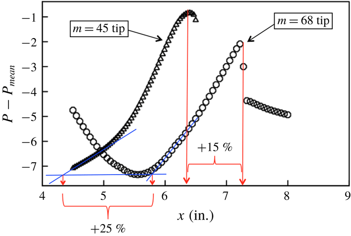
line, indicating that the transition Reynolds number has increased. As further evidence, the method of Schuele et al. (Reference Schuele, Corke and Matlis2013) was used to estimate transition location. This involved following the
 $x$
-trajectory of a minimum in the total pressure distributions in figures 11(a) and 13(a). The actual trajectories are shown by the dotted curves in those two figures. As previously mentioned, the pressure minima are indicative of a region of local thickening of the boundary layer. Such regions are known to develop an off-wall inflectional shear layer and subsequent inviscid instability that quickly leads to turbulence (Craig & Saric Reference Craig and Saric2016). The starting azimuthal locations of both of these trajectories
 $(138^{\circ }\leqslant \unicode[STIX]{x1D703}\leqslant 140^{\circ })$
is where the
 $N$
-factor
 $=$
10 curve is furthest upstream on the cone and therefore where transition is expected to occur first.
The
 $x$
-development of the total pressure along the two pressure minima for the ‘critical’ (
 $m=45$
) and ‘subcritical’ (
 $m=68$
) roughness is shown in figure 14. Estimates of the transition location were performed by two approaches. The first, shown in blue, followed a Preston tube approach in which a linear curve is fit to the rise in the total pressure near the wall that would accompany transition. The
 $x$
-location where the linear curve intersects a common reference level is designated as the transition location. Based on this approach, the subcritical roughness resulted in a 25 % increase in the transition location.
The second approach is based on the loss in the coherence of the mean flow distortion. This would be evident as saturation and abrupt decay in the axial development of the total pressure. Based on this approach, shown in red, the subcritical roughness pattern resulted in a 15 % increase in the transition location. Schuele et al. (Reference Schuele, Corke and Matlis2013) considered this as an indication of the late stage of transition, whereas the Preston tube approach was considered to be an indication of the early stage of transition.

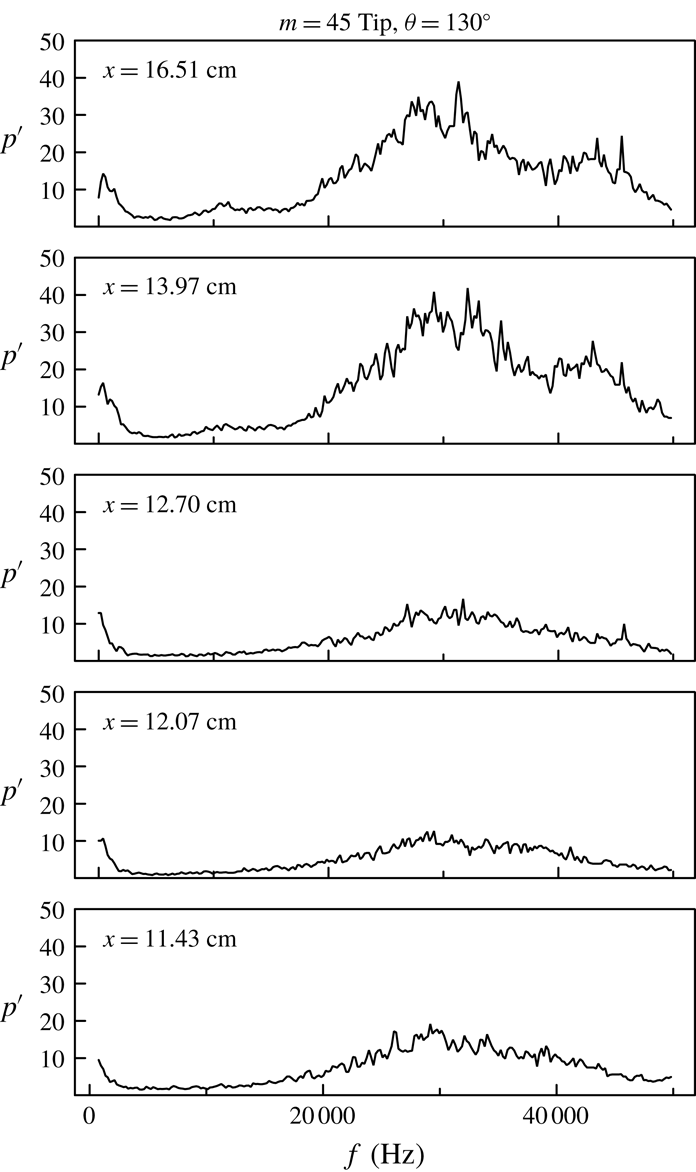
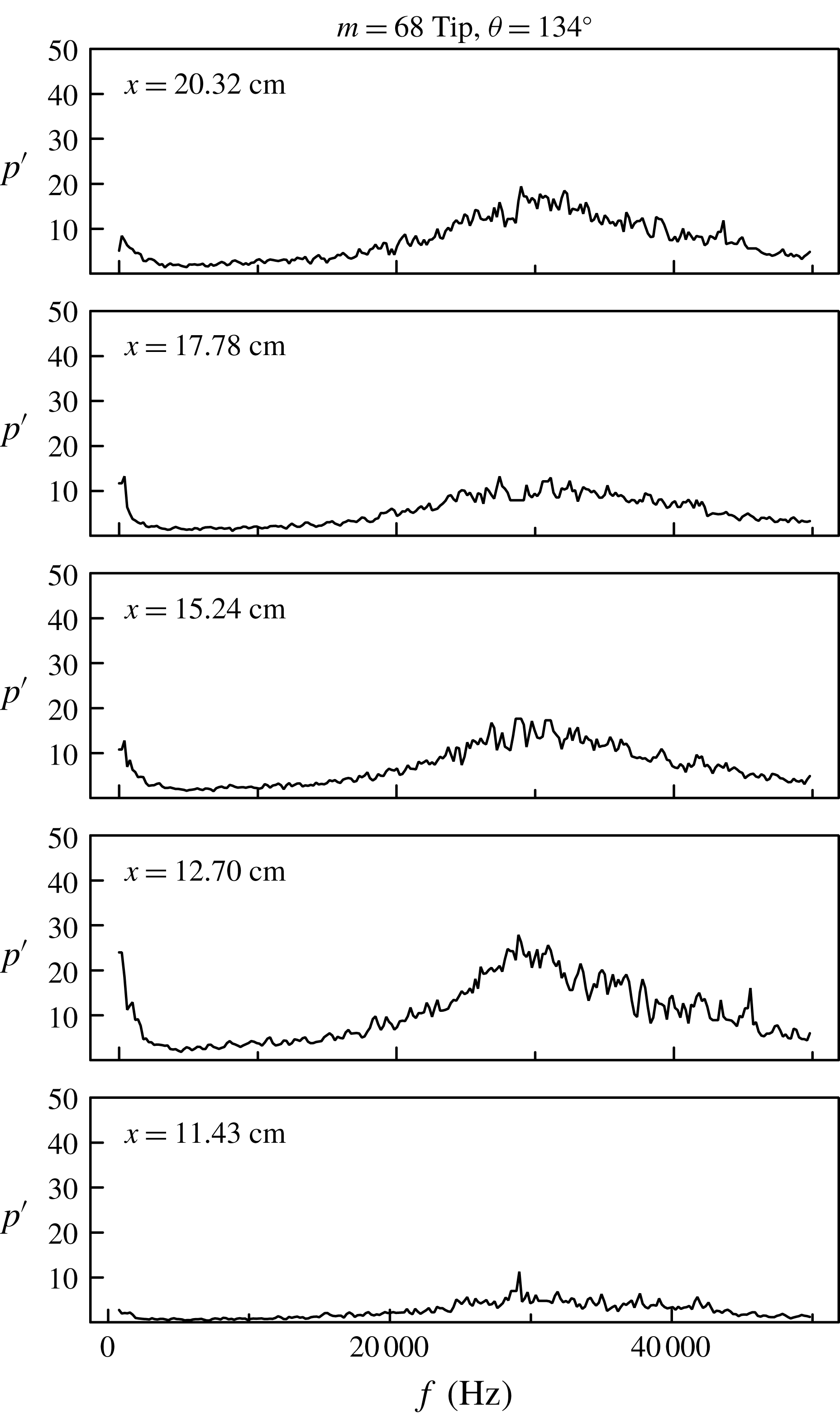
As mentioned, the total pressure Pitot probes had a frequency response that was capable of detecting the travelling cross-flow modes. Figures 15 and 16 show spectra of off-wall total pressure fluctuations at increasing
 $x$
locations for a single azimuthal angle for the critical and subcritical roughness cone tips. Both of these show a broad peak that is centred near 30 kHz that was predicted to be the frequency of the most-amplified travelling cross-flow modes (Li et al.
Reference Li, Choudhari, Chang and White2010). The azimuthal wavenumber of the most-amplified travelling mode is predicted (Li et al.
Reference Li, Choudhari, Chang and White2010) to be
 $m=40$
.
Spectra of travelling disturbances measured at different axial locations for a constant azimuthal angle for the ‘critical’ (
 $m=45$
) roughness.

Spectra of travelling disturbances measured at different axial locations for a constant azimuthal angle for the ‘subcritical’ (
 $m=68$
) roughness.

The peak values of the spectra of the travelling disturbances, for all of the measured
 $(\unicode[STIX]{x1D703},x)$
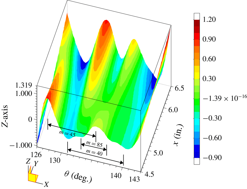
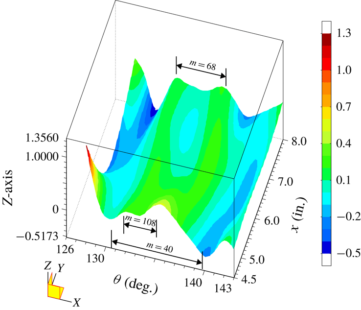
locations for the two tip roughness cases, were used to compile a view of the spatial amplitude distribution for the travelling cross-flow modes. These are shown for the critical
 $m=45$
roughness cone tip in figure 17, and for the subcritical
 $m=68$
roughness cone tip in figure 18. Examination of these reveals the presence of features with different azimuthal wavenumbers. To interpret these, one needs to consider possible interactions between the travelling and stationary cross-flow modes.
Spatial amplitude distribution of the spectral peak amplitude of the travelling disturbances for the ‘critical’ (
 $m=45$
) roughness tip.

Spatial amplitude distribution of the spectral peak amplitude of the travelling disturbances for the ‘subcritical’ (
 $m=68$
) roughness tip.

Physically, the travelling cross-flow modes ride (convect) over the stationary modes which then have the potential to modulate and interact with the travelling modes. Corke & Knasiak (Reference Corke and Knasiak1998a ), Corke & Matlis (Reference Corke and Matlis2006) and Corke et al. (Reference Corke, Matlis and Othman2007) documented a nonlinear (quadratic) sum and difference interactions between travelling and stationary cross-flow modes in 3-D boundary layers over a rotating disk. The question is if there is similar interaction occurring in this instance.
Considering the ‘critical’ roughness cone tip, the stationary modes were documented to occur at
 $m=45$
. This mode will be designated as
 $(0,45)$
, where the first index is the frequency, and the second is the azimuthal wavenumber. Li et al. (Reference Li, Choudhari, Chang and White2010) determined the most-amplified travelling cross-flow mode occurred with an azimuthal wavenumber of
 $m=40$
. This mode will be designated as
 $(f_{t},40)$
, where
 $f_{t}$
refers to the frequency of the travelling mode which figures 15 and 16 found to be centred on 30 kHz.
The first interaction between these two modes will be through a sum and difference, namely
 $$\begin{eqnarray}(0,45)\pm (f_{t},40)=(f_{t},85)\quad \text{and}\quad (f_{t},5).\end{eqnarray}$$
Both
 $(f_{t},85)$
and
 $(f_{t},5)$
are travelling modes with the same frequency as the primary travelling mode. Therefore the amplitude of the spectral peak in figure 17 should be representative of not only the primary travelling mode, but also the sum and difference modes that occur at the same frequency.
Now the result of the summing interaction,
 $(f_{t},85)$
, would have an azimuthal wave angle of approximately
 $4^{\circ }$
. That of the difference interaction,
 $(f_{t},5)$
, would have an azimuthal wave angle of
 $72^{\circ }$
. The latter is larger than the azimuthal extent of the measurements. However the former,
 $(f_{t},85)$
, is distinguishable in the spatial amplitude distribution in figure 17.
Also observable is a spatial amplitude distribution with an azimuthal wavenumber that matches that of the discrete roughness,
 $m=45$
. This is not realizable through a quadratic interaction to produce
 $(f_{t},45)$
. Therefore it is most likely due to a linear superposition that leads to a modulation of the travelling mode amplitude as it rides over the stationary mean flow distortion. Such behaviour has in fact been identified through direct Navier–Stokes simulations of subsonic 3-D boundary layers undergoing cross-flow instability by Dörr, Kloker & Hanifi (Reference Dörr, Kloker and Hanifi2017).
For the case with the ‘subcritical’,
 $m=68$
roughness cone tip, the sum and difference interaction would be
 $$\begin{eqnarray}(0,68)\pm (f_{t},40)=(f_{t},108)\quad \text{and}\quad (f_{t},28).\end{eqnarray}$$
Here
 $(f_{t},108)$
would have an azimuthal wave angle of approximately
 $3^{\circ }$
, and
 $(f_{t},28)$
an azimuthal wave angle of approximately
 $13^{\circ }$
. Both again are travelling modes with the same frequency as the primary travelling mode. Both of these are evident in the spatial amplitude distribution shown in figure 18.
As before, a spatial amplitude distribution with an azimuthal wavenumber that matches that of the discrete roughness,
 $m=68$
, is also observable. This again is most likely due to a linear superposition that produces a modulation of the travelling mode amplitude as it rides over the stationary mean flow distortion produced by the
 $m=68$
roughness.
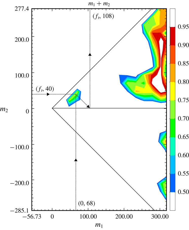
An attempt has been made to quantify these sum and difference interactions by determining the degree of phase locking between the primary stationary and travelling cross-flow modes and their sum and difference modes. This utilized the cross-bicoherence statistic previously used in documenting nonlinear interaction between stationary and travelling cross-flow modes in the boundary layer over a rotating disk (Corke & Matlis Reference Corke and Matlis2006; Corke et al. Reference Corke, Matlis and Othman2007). The cross-bicoherence (CBC) is defined as
 $$\begin{eqnarray}\unicode[STIX]{x1D6FD}_{ijk}(m_{1},m_{2})=\frac{|\tilde{R}_{ijk}(m_{1},m_{2})|^{2}}{\langle |\tilde{p}_{i}(m_{1})|^{2}|\tilde{p}_{j}(m_{2})|^{2}\rangle \langle |\tilde{p}_{k}(m_{3})|^{2}\rangle },\end{eqnarray}$$
where
 $$\begin{eqnarray}\tilde{R}_{ijk}(m_{1},m_{2})=\langle \tilde{p}_{i}(m_{1})\tilde{p}_{j}(m_{2})\tilde{p}_{k}^{\ast }(m_{3})\rangle\end{eqnarray}$$
is the cross-bispectrum, with
 $i$
,
 $j$
and
 $k$
equal to either
 $i$
or
 $j$
that refer to one of the two mean-removed pressure time series,
 $p$
, with azimuthal wavenumbers
 $m_{1}$
,
 $m_{2}$
and
 $m_{3}$
, respectively. The notation (
 $|\,|$
) is the modulus of the component,
 ${\sim}$
denotes the Fourier transformed function in wavenumber domain,
 $\langle \,\rangle$
represents the ensemble average. These wavenumbers are related to each other such that
 $m_{1}+m_{2}+m_{3}=0$
.
In the experiment, one of the data series used in the CBC was the azimuthal variation in the time-averaged total pressure,
 $\bar{p}(\unicode[STIX]{x1D703})$
, at a selected
 $x$
location on the cone. The same data were used to generate figures 11(a) and 13(a). This data series therefore represents the azimuthal mean flow distortion at one
 $x$
location. The Fourier transform of this data series is
 $\tilde{\bar{p}}(m)$
. The wavenumber spectra shown in figures 11(b) and 13(b) correspond to
 $|\tilde{\bar{p}}(m)|^{2}$
at each
 $x$
location.
The second data series used in the CBC corresponds to the total pressure time series before time averaging,
 $p(t)(\unicode[STIX]{x1D703})$
, at the same
 $x$
location as
 $\bar{p}(\unicode[STIX]{x1D703})$
. This data series contains pressure fluctuations that correspond to the travelling cross-flow modes. The squared modulus of the transformed data series,
 $|\tilde{p}(f)|^{2}$
, was used to generate the frequency spectra that are shown in figures 15 and 16.
It is necessary that the two transformed data series have the same independent variable units. In
 $|\tilde{p}(m)|^{2}$
, the independent variable is azimuthal wavenumber,
 $m$
. In
 $|\tilde{p}(f)|^{2}$
the independent variable is frequency,
 $f$
. Therefore in the case of the latter, we chose to convert frequency to azimuthal wavenumber. As previously pointed out, analysis from Li et al. (Reference Li, Choudhari, Chang and White2010) indicated that the azimuthal wavenumber in the centre of the most amplified band of frequencies of travelling cross-flow mode (35 kHz) was
 $m=40$
. This was used as a point of reference to the conversion from frequency to wavenumber of the travelling mode data series.
Another important step in computing the CBC was that the sampling rates be the same for the two data series. For the time series representing the stationary cross-flow mode,
 $\bar{p}(\unicode[STIX]{x1D703})$
(data series 1), the sampling rate was
 $8.54~\text{pts}/\circ$
. For the time series representing the travelling cross-flow mode (data series 2), the sampling rate was considerably less at
 $0.317~\text{pts}/\circ$
. Therefore in order to match the two data sampling rates, data series 2 was zero padded by the appropriate amount prior to the Fourier transform.
As with linear coherence, the value of the CBC varies between 0 and 1. High values of the CBC indicate a high degree of triple phase locking
 $$\begin{eqnarray}\unicode[STIX]{x1D703}_{i}(m_{1})+\unicode[STIX]{x1D703}_{j}(m_{2})=\unicode[STIX]{x1D703}_{k}(m_{3})\end{eqnarray}$$
from realization to realization. Here
 $\unicode[STIX]{x1D703}_{i}(m_{1})$
is the instantaneous circular phase angle of
 $\tilde{p}_{i}(m_{1})$
.
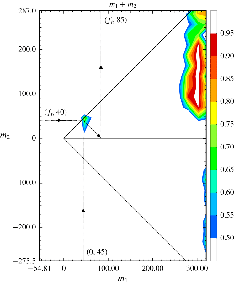
The region of validity of the CBC is set by the Nyquist criterion, where the sum of any two frequencies (or wavenumbers in this case) cannot exceed half the sampling rate. This region then takes the form of two isosceles triangles, one each for sum and difference interactions. The outline of the two triangles defining the valid regions is shown in figures 19 and 20. The region of interest has been enlarged to focus on the two summing interactions between the stationary and travelling cross-flow modes that was postulated for the ‘critical’ and ‘subcritical’ roughness tips.
For the CBC shown in figures 19 and 20, the data series 1 corresponding to the stationary cross-flow modes is designated by subscript 1, with its wavenumber read from the abscissa. The data series corresponding to the travelling cross-flow modes is designated by subscript 2, with its wavenumber read from the ordinate. The ordinate wavenumbers are either added (top triangle) or subtracted (bottom triangle) from those read on the abscissa to give the third frequency which is read as the intercept of a
 $-45^{\circ }$
line to the abscissa. This method for reading the CBC is outlined by the yellow arrows for the summing interaction in the two figures.
The decision of which of the two data series (1 or 2) corresponds to the
 $i$
,
 $j$
and
 $k$
series in the calculation of
 $\unicode[STIX]{x1D6FD}_{ijk}(m_{1},m_{2})$
in equation (3.3) is important. For example if
 $[i,j,k]=[1,1,1]$
the CBC would indicate wavenumbers in data series 1 that result from sum and difference interactions in data series 1. This is referred to as the auto-bicoherence. Similarly this could only involve data series 2 where
 $[i,j,k]=[2,2,2]$
. Based on the results in figures 17 and 18, that indicate an influence of the stationary cross-flow mode on the spatial amplitude distribution of the travelling cross-flow mode, we chose the order
 $[i,j,k]=[1,2,2]$
. Thus we were investigating an interaction between the stationary mode, 1, and the travelling mode, 2, that results in sum and difference travelling modes, 2.
CBC for ‘critical’ roughness case indicating triple phase locking for
 $(0,45)+(f_{t},40)=(f_{t},85)$
. Measured at
 $(x,\unicode[STIX]{x1D703})=(4.5~\text{in.},135^{\circ })$
.

CBC for ‘subcritical’ roughness case indicating triple phase locking for
 $(0,68)\pm (f_{t},40)=(f_{t},108)$
. Measured at
 $(x,\unicode[STIX]{x1D703})=(4.5~\text{in.},138^{\circ })$
.

The CBC statistic involved 256 ensembles. Figure 19 corresponds to the ‘critical’ roughness case. The (
 $x,\unicode[STIX]{x1D703}$
) location corresponds to the most upstream measured location (
 $x=11.43~\text{cm}$
), and an azimuthal location (
 $\unicode[STIX]{x1D703}=135^{\circ }$
) where the spatial amplitude at the centre frequency of the travelling cross-flow mode (35 kHz) was at a peak level as shown in figure 17. The CBC at that location indicates a significant triple phase locking between the stationary cross-flow mode generated by the ‘critical’ (
 $m=45$
) roughness, and the travelling cross-flow mode with azimuthal wavenumber (
 $m=40$
) to produce a travelling cross-flow mode with an azimuthal wavenumber of
 $m=85$
. This is a strong indication that the
 $m=85$
variation in the spatial amplitude distribution in figure 17 is the result of a nonlinear interaction between the stationary and travelling cross-flow modes.
The CBC does not reveal the difference interaction between the stationary and travelling modes that would result in the travelling mode at
 $m=5$
. The azimuthal span of the measurements in figure 17 was insufficient to indicate if there was an azimuthal amplitude variation of this travelling mode with this mode number. Therefore based on the CBC alone, there is no evidence of this difference interaction.
Finally the CBC reveals strong triple phase locking in summing interactions between higher stationary wavenumbers and a broad range of wavenumbers of travelling modes. The higher stationary wavenumbers might represent uncontrolled surface roughness on the cone tip. If this is the case, it points to a mechanism for spectral broadening. However, a large CBC only indicates phase locking. It does not indicate the level of energy in these modes. Based on the spectra that were shown in figure 15, the dominant travelling mode is centred near 30 kHz and associated with
 $m=40$
.
The CBC for the ‘subcritical’ roughness case is shown in figure 20. The (
 $x,\unicode[STIX]{x1D703}$
) location again corresponds to the most upstream measured location (
 $x=11.43~\text{cm}$
). The azimuthal location was
 $\unicode[STIX]{x1D703}=138^{\circ }$
, which was close to the spatial amplitude peak at that
 $x$
-location in figure 18, and aligned with the peak having the discrete roughness
 $m=68$
spacing at the downstream location. In this case, the CBC indicates a significant triple phase locking between the stationary cross-flow mode generated by the ‘subcritical’ (
 $m=68$
) roughness, and the travelling cross-flow mode with azimuthal wavenumber (
 $m=40$
) to produce a travelling cross-flow mode with an azimuthal wavenumber of
 $m=108$
. Therefore there is a strong indication of a nonlinear interaction between the stationary and travelling cross-flow modes that in this case results in a travelling mode with an azimuthal wavenumber of
 $m=108$
.
The azimuthal amplitude distribution for the travelling cross-flow mode in figure 18 had also revealed a variation with azimuthal wavenumber of
 $m=28$
that could have been the result of a nonlinear difference interaction between the stationary and travelling cross-flow modes. As with the previous case, the CBC in figure 20 does not reveal a difference interaction leading to
 $m=28$
. As with the previous case, the CBC indicates strong triple phase locking between higher stationary mode azimuthal wavenumbers and a broad band of travelling mode wavenumbers. As before, based on the travelling mode spectra in figure 16, the lower energy in these higher mode numbers makes it more likely that the phase locked interactions near the most-amplified travelling mode wavenumber will dominate at transition.
4 Discussion
The surface flow visualization and off-wall azimuthal surveys of the total pressure revealed the same picture of the mean flow distortion produced by the stationary cross-flow modes that developed in the boundary layer over the right-circular cone at the
 $6^{\circ }$
angle of attack. These measurements confirmed the receptivity of the cross-flow mode to the discrete roughness in a conventional (non-quiet design) environment.
The design of the roughness was identical in all characteristics to that used by Schuele et al. (Reference Schuele, Corke and Matlis2013) in a quiet Mach 3.5 tunnel. The passive roughness consisted of micron-sized indentations (dimples) that were located near the cone tip, just upstream of the first neutral growth branch of stationary cross-flow modes, based on linear stability analysis. The roughness dimples encircled the cone tip with a uniform spacing that defined the azimuthal wavenumber of the roughness. The disturbances produced by the roughness dimples were expected to follow the theoretical vortex path lines to the azimuthal region where turbulent transition was predicted to first occur based on linear theory
 $N$
-factors. For the cone at a
 $6^{\circ }$
angle of attack, this was expected to be in the range of azimuthal angles from
 $110^{\circ }$
to
 $150^{\circ }$
, measured from the windward stagnation line. As a result, although the dimples encircled the cone tip, only those that intersected with the theoretical vortex path lines at the axial location of the roughness were active.
Two azimuthal wavenumbers of roughness were investigated. One was in the band of the initially most-amplified (‘critical’) wavenumbers of stationary cross-flow modes. The other was at a 1.5 times higher (‘subcritical’) wavenumber. The ‘critical’ wavenumber roughness was intended to represent a controlled baseline that would favour a single wavenumber stationary cross-flow mode. The ‘subcritical’ wavenumber roughness was intended to suppress the growth of initially amplified stationary cross-flow modes and thereby increase the transition Reynolds number in a scenario first documented at subsonic Mach numbers by Saric et al. (Reference Saric, Ruben and Reibert1998).
A smooth cone tip representing an uncontrolled baseline was documented only through surface flow visualization. This was the only viable approach for a full-field survey without a defined roughness pattern that was fixed from one run to the next in the Ludwieg tube. This however did reveal a stationary pattern with azimuthal wavenumbers that were in the band predicted to be most amplified from linear theory by which our ‘critical’ roughness was selected. The transition location with the smooth tip was also in good agreement with that for the critical roughness, suggesting that the disturbance amplitude of the critical roughness was comparable to that of random roughness on the smooth tip.
Transition for the smooth cone tip, and that with the ‘critical’ roughness, indicated an
 $N$
-factor of 10 near transition. This was similar to that observed by Schuele et al. (Reference Schuele, Corke and Matlis2013) in a ‘quiet’ Mach 3.5 flow. One might expect that in the present results in the conventional non-quiet AFA tunnel, transition might occur earlier compared to the quiet tunnel. The free-stream disturbances could be any combination of entropy, vorticity and acoustic fluctuations, however in hypersonic tunnels, vorticity is highly stretched and damped leaving primarily entropy and acoustic fluctuations. With regard to stationary cross-flow modes, evidence at subsonic Mach numbers indicates a lack of sensitivity to acoustic disturbances (Radeztsky et al.
Reference Radeztsky, Reibert and Saric1999). Therefore we might not expect any difference between the cross-flow transition
 $N$
factors for ‘quiet’ and ‘noisy’ tunnels. The results appear to support that conclusion.
A corollary to that discussion is that in the process of transition of the stationary cross-flow modes, the resulting mean flow distortion develops high shear layers (Craig & Saric Reference Craig and Saric2016) that are then inviscidly unstable, and susceptible to acoustic disturbances. Therefore this might provide a mechanism by which transition might be hastened in a conventional, non-quiet, tunnel. However being an inviscid instability, the high amplification rate would lead to a rapid transition in a short distance that could be imperceptible in comparison to that in a ‘quiet’ tunnel.
Transition front measurements using the Preston tube approach indicated that the transition Reynolds number had increased by approximately 25 % with the ‘subcritical’ wavenumber roughness compared to the ‘critical’ wavenumber roughness. This is less than the 40 % increase in the transition Reynolds number in the Mach 3.5, quiet environment documented by Schuele et al. (Reference Schuele, Corke and Matlis2013). Given that the roughness design was the same in both experiments, one can question if
(i) the difference in the increase in transition Reynolds number was due to a Mach number effect, or
(ii) if the difference is due to the difference in acoustic disturbance levels between the experiments.
With regard to the latter, Neel et al. (Reference Neel, Leidy, Tichenor and Bowersox2018) have investigated the effect of free-stream disturbances on stationary cross-flow modes on elliptic cones. The disturbance levels were varied based on the position of the model within the nozzle expansion. The presence of stationary cross-flow modes was determined by thermal imaging where they appeared as elevated temperature streaks. They observed that the lower disturbance level produced more distinct streaks compared to the higher disturbance condition. Neel et al. (Reference Neel, Leidy, Tichenor and Bowersox2018) observed that the streak formation at their lower disturbance condition compared well with that obtained on the same geometric model under ‘quiet’ conditions (Juliano & Schneider Reference Juliano and Schneider2010).
Neel et al. (Reference Neel, Leidy, Tichenor and Bowersox2018) had also investigated transition on their elliptic cone model in a ‘quiet’ tunnel. The thermal images revealed extremely sharp hot streaks that suggested well defined stationary cross-flow vortices. Model surface pressure measurements in the quiet tunnel environment showed energy in a band of frequencies centred about 40 kHz. that is expected to be due to travelling cross-flow modes.
The locations of the streaks in the thermal images, associated with the stationary cross-flow modes in the Neel et al. (Reference Neel, Leidy, Tichenor and Bowersox2018) experiments did not always coincide with the azimuthal locations of the surface pressure sensors. This then offered a means of assessing any azimuthal variation in the amplitude of the 40 kHz travelling cross-flow mode in their experiments. In particular, their Run 3180 reveals such an azimuthal variation that could be evidence of an interaction between the travelling and stationary cross-flow modes.
The origin of the stationary cross-flow modes in experiments like those of Neel et al. (Reference Neel, Leidy, Tichenor and Bowersox2018), and Juliano & Schneider (Reference Juliano and Schneider2010) are expected to be due to randomly distributed surface roughness. In contrast, the patterned discrete roughness used in the experiments by Schuele et al. (Reference Schuele, Corke and Matlis2013) and the present experiments was fixed. This controlled roughness initial condition offered a more quantitative approach to explore possible interactions between the travelling and stationary cross-flow modes. Such an approach followed that used by Corke & Matlis (Reference Corke and Matlis2006) and Corke et al. (Reference Corke, Matlis and Othman2007) in the canonical cross-flow transition that occurs on a rotating disk.
The evidence of an interaction between the stationary and travelling cross-flow modes is embodied in the spatial amplitude distributions for the two roughness cases that was shown in figures 17 and 18. Recalling that these were the result of hundreds of individual wind tunnel runs, with the only constant, besides Reynolds number, being the controlled discrete roughness on the model, the coherent pattern in the spatial fluctuation amplitude is remarkable.
The spatial amplitude distribution showed evidence of a quadratic interaction between the linearly amplified travelling and stationary cross-flow modes. For the critical roughness with frequency and mode number of
 $(0,45)$
, this led to the generation of a travelling mode
 $(f_{t},85)$
with the same frequency as the primary travelling mode,
 $f_{t}$
. The quadratic interaction between
 $(f_{t},85)$
and the stationary and the primary travelling modes was confirmed with the CBC statistic. The
 $(f_{t},85)$
mode resulted from a summing interaction. One would expect a similar difference interaction that would lead to a travelling mode
 $(f_{t},5)$
. However, this was not confirmed in the experiment. If the difference mode,
 $(f_{t},5)$
, were to occur, then an interaction with the summed mode,
 $(f_{t},85)$
, could produce a harmonic travelling mode,
 $(2f_{t},90)$
, and a higher wavenumber stationary mode,
 $(0,80)$
. Evidence of the latter might be found in the thermal images of Neel et al. (Reference Neel, Leidy, Tichenor and Bowersox2018) or Juliano & Schneider (Reference Juliano and Schneider2010).
This process of successive interactions can be a mechanism to spread energy that leads to a broad spectrum associated with turbulence. Such a broadening spectrum was apparent in the wavenumber spectra based on the surface flow visualization and off-wall pressure measurements that were shown in figures 9 and 10, and figures 11(b) and 13(b) for the discrete roughness cases.
The strength of these interactions will depend on the initial amplitude of the travelling cross-flow modes. Evidence indicates that this depends on the free-stream disturbance level that particularly includes vortical disturbances, and possibly acoustic disturbances. If one excludes Mach number effects, the difference between the degree of transition suppression between the experiments of Schuele et al. (Reference Schuele, Corke and Matlis2013) and the present experiments is likely only the level of acoustic disturbances. The potentially larger amplitude travelling cross-flow modes in the higher acoustic environment, and the nonlinear interaction with the stationary mode, could hasten transition, and reduce the effectiveness of the subcritical roughness. In a broader sense, this interaction between stationary and travelling cross-flow modes might account for the difference between the transition Reynolds number in conventional (noisy) and quiet hypersonic wind tunnels.
5 Conclusions
Experiments in the 3-D boundary layer on a right-circular cone at an angle of attack demonstrated the receptivity of stationary cross-flow modes to passive patterned roughness at Mach 6.0. The experiments were performed in a Ludwieg tube that included a conventional nozzle that was not designed to suppress acoustic disturbances. The passive roughness consisted of micron-sized indentations (dimples) that were located near the cone tip, just upstream of the first neutral growth branch of stationary cross-flow modes, based on linear stability theory. The roughness dimples encircled the cone tip with a uniform spacing that defined the azimuthal wavenumber of the roughness. Roughness with two different azimuthal wavenumbers were investigated. The first was at a ‘critical’ wavenumber that was approximately centred in the band of the most-amplified stationary cross-flow modes. The other was at a ‘subcritical’ wavenumber that was 1.5 times higher than the ‘critical’ wavenumber, and intended to increase the transition Reynolds number. A smooth cone tip representing an uncontrolled baseline was used to substantiate linear theory predictions and to provide contrast to the critical wavenumber roughness case.
The results confirmed that the stationary cross-flow mode was receptive to the passive patterned roughness. Transition front measurements using the Preston tube approach indicated that the transition Reynolds number had increased by 25 % with the ‘subcritical’ wavenumber roughness. This compared to a 40 % increase in the transition Reynolds number using the same cone model and discrete roughness approach at Mach 3.5 in a ‘quiet’ tunnel by Schuele et al. (Reference Schuele, Corke and Matlis2013). The question remains if this difference is due to the difference in Mach number, or to the free-stream acoustic disturbance level.
The prescribed roughness initial conditions revealed evidence of a nonlinear (quadratic) interaction between the stationary and travelling cross-flow modes. This appeared as an azimuthal variation in the amplitude of the travelling cross-flow mode with azimuthal wavenumbers that corresponded to the sum and difference of the azimuthal wavenumbers of the primary stationary and travelling modes. Cross-bicoherence verified a triple phase locking between the two primary modes and the summed mode for both the ‘critical’ and ‘subcritical’ roughness cases. The triple phase locking for the difference mode interaction was not evident in the CBC. This was possibly due to the limited azimuthal extent required to resolve the low azimuthal wavenumbers.
The impact that this nonlinear interaction has on transition will depend on the initial amplitude of the travelling modes. The amplitudes of travelling cross-flow modes are expected to depend on the free-stream disturbance level. This may then offer a mechanism to explain the variation in cross-flow dominated transition Reynolds numbers in different facilities.
Acknowledgement
This work was supported by the Air Force Office of Scientific Research under grant FA9550-15-1-0278 that is monitored by Dr I. Leyva.