

1 Introduction
A problem of considerable interest in the theory of canonical turbulent free shear flows is the description of the far field of turbulent planar jets. For a Newtonian fluid, a vast amount of knowledge obtained from carefully conducted experiments and numerical simulations is available and a theory of the turbulent plane jet has been established (Tennekes & Lumley Reference Tennekes and Lumley1972; Townsend Reference Townsend1976; Pope Reference Pope2000), even if recently, this classical theory has been challenged by a number of experimental and numerical works (Layek & Sunita Reference Layek2018; Sadeghi, Oberlack & Gauding Reference Sadeghi, Oberlack and Gauding2018; Cafiero & Vassilicos Reference Cafiero and Vassilicos2019).
The situation is very different when one considers canonical turbulent free shear flows of viscoelastic fluids. Specifically, there is presently no theory for the behaviour of turbulent planar jets of viscoelastic fluids. Since the discovery that the addition of very small amounts of polymer additives to a Newtonian solvent can result in a substantial decrease in the friction drag, a lot of effort has been put to understanding and describing turbulence in viscoelastic fluids, but unfortunately these efforts have been mainly focused on viscoelastic fluid flows in the presence of walls.
Due to the dramatic drag reduction observed in wall turbulence of viscoelastic fluids, the first experimental studies of turbulent viscoelastic jets were aimed at investigating the origin of the drag reduction, and to understanding to what extent this phenomenon is exclusive to wall turbulence. However, contradictory conclusions were obtained in these early studies. Visualisations showed a dramatic suppression of small-scale disturbances in viscoelastic jets, compared to Newtonian jets, and a reduction in the jet spreading rate, combined with a slower transition to turbulence (Gadd Reference Gadd1965, Reference Gadd1966; White Reference White and Wells1969, Reference White1972; Wu Reference Wu and Wells1969; Shul’Man et al. Reference Shul’Man, Pokryvailo, Kovalevskaya and Kulebyakin1973; Hoyt, Taylor & Runge Reference Hoyt, Taylor and Runge1974; Filipsson, Lagerstedt & Bark Reference Filipsson, Lagerstedt and Bark1977; Usui et al. Reference Usui, Sano, Kawata and Sakai1980; Gyr Reference Gyr1996). On the other hand, quantitative measurements have indicated that in the far field the flow is unaffected by the polymers (Goren & Norbury Reference Goren and Norbury1967; Jackley Reference Jackley1967; Pownall & Kiser Reference Pownall and Kiser1970; Serth & Kiser Reference Serth and Kiser1970; Barker Reference Barker1973), or that the spreading rate is actually an increasing function of the polymer concentration (White Reference White1967).
Except for Barker (Reference Barker1973), all these early measurements were made using Pitot tubes or hot-film anemometers, which are now known to give erroneous results for flows of viscoelastic fluids. However, Usui et al. (Reference Usui, Sano, Kawata and Sakai1980) employed tracer particles visualisation techniques and obtained mean and fluctuating profiles of velocity that show a decrease in the turbulent shear stresses and turbulence intensities, and an increase in the integral length scale of the turbulence in the streamwise direction, compared to classical Newtonian jets. Usui et al. (Reference Usui, Sano, Kawata and Sakai1980) also measured the evolution of the centreline mean velocity with Pitot tubes and observed an increased decay rate, compared with a Newtonian jet. In contrast, the velocity measurements of Berman & Tan (Reference Berman and Tan1985) with a laser Doppler anemometer (LDA) showed the opposite trends regarding the centreline velocity decay and the turbulent intensity. Slower decaying and spreading rates (compared to the Newtonian jet) were also observed by Koziol & Glowacki (Reference Koziol and Glowacki1989), who employed an electromechanical technique to measure the velocity field. Vlasov, Isaeva & Kalashnikov (Reference Vlasov, Isaeva and Kalashnikov1973) also performed LDA measurements of the velocity field in turbulent jets of viscoelastic fluids and observed that the centreline velocity decay rate is not affected by the polymers, while the turbulent intensity is slightly increased. Finally, Berman (Reference Berman1986) obtained budgets of turbulent kinetic energy in turbulent jets of viscoelastic fluids, showing that the viscous dissipation rate is not affected by the polymers, while the turbulent transport is highly affected. However, his calculations were performed with expressions valid for turbulent flows of Newtonian fluids, that are not in general valid for viscoelastic fluids.
From the above description, it is clear that the behaviour of turbulent viscoelastic jets is still largely an open problem in the turbulence and fluid dynamics community, and that needs to be addressed. It is frustrating to see that the experimental studies show contradictory conclusions, and that this problem does not appear to have been addressed before in any systematic way, either theoretically or numerically. In the present paper, we carry out new direct numerical simulations (DNS) of turbulent planar jets of dilute polymer solutions, described by the finitely extensible nonlinear elastic constitutive equation closed with the Peterlin approximation (FENE-P), to investigate these flows, and to develop a theory for the far-field, fully developed region of turbulent jets of viscoelastic fluids. For simplicity, we address the case of the planar jet, instead of the more commonly found circular or round jet configuration.
Thanks to the new DNS the effects of the polymer molecules on the jet statistics can be easily accessed, and can be used to derive expressions for the spreading rate, centreline velocity decay rate and maximum polymer stresses decay rate along the streamwise direction of the jet. To the authors’ knowledge the expressions derived in this work consist of the first systematic attempt towards developing a theory for the turbulent planar jet of a viscoelastic fluid.
The new theory developed here to describe the far field of viscoelastic turbulent planar jets is largely based on the arguments put forward by Lumley (Reference Lumley1973), and independently recovered by Seyer & Metzner (Reference Seyer and Metzner1969), and makes no use of the FENE-P rheological model used in the present simulations, and therefore should in principle be valid to describe turbulent planar jets of any viscoelastic fluid.
This paper is organised as follows. Section 2 introduces the governing equations, numerical methods and the physical and computational parameters of the simulations carried out in the present study. Section 3 describes the main features of turbulent viscoelastic jets, compared with ‘classical’ Newtonian jets. In § 4 a new theory for turbulent viscoelastic jets is proposed and assessed with existing data. The work ends in § 5 with an overview of its main results and conclusions.
2 Direct numerical simulations of viscoelastic turbulent planar jets
A total of 12 direct numerical simulations of viscoelastic turbulent planar jets were carried out in the present work, that basically differ in the polymer concentration and the relaxation time of the polymer molecules. Additionally, a reference DNS of a Newtonian turbulent planar jet was carried out for comparison. The simulations use the FENE-P rheological model and are carried out with a very accurate numerical code described below.
2.1 The FENE-P fluid governing equations
The DNS are designed to simulate turbulent planar jets of a Newtonian solvent carrying a large number of long chain polymer molecules, representing, however, a very small fraction of the total fluid i.e. a diluted polymeric solution. To represent the rheological behaviour of the polymeric solutions, use is made of the finitely extensible nonlinear elastic constitutive model closed with Peterlin’s approximation i.e. the FENE-P rheological model proposed by Bird, Dotson & Johnson (Reference Bird, Dotson and Johnson1980). The FENE-P model is known to offer a good trade-off between rheological fidelity and computational demand in turbulence simulation studies. It has a solid theoretical background, based on the kinetic theory of polymeric liquids (Bird et al. Reference Bird, Curtiss, Armstrong and Hassager1987), where the macroscopic behaviour of a large ensemble of polymer molecules is represented by a simple model of the polymeric chains. In this model the effect of a large number of polymer molecules is represented by a single spring connecting two beads (the so-called dumbbell), with a nonlinear force law that prevents over-extension of the chain when large forces are applied. The FENE-P model has four parameters: the kinematic viscosity of the polymer  $\unicode[STIX]{x1D708}^{[p]}$, the solvent viscosity ratio
 $\unicode[STIX]{x1D6FD}$ (defined below), the maximum relaxation time of the polymer molecules
 $\unicode[STIX]{x1D70F}_{p}$ and the square of the maximum extensibility of the polymer molecules, normalised by the square of the equilibrium radius of the chain
 $\langle R^{2}\rangle _{0}$ (the brackets denote an ensemble average over all configurations of the chain),
 $L^{2}$.
The effect of the polymer molecules on the equations governing the flow is encapsulated in the polymer stress tensor  $\unicode[STIX]{x1D748}^{[p]}$, that appears as an extra stress in the momentum equation for the solution,
 $$\begin{eqnarray}\frac{\unicode[STIX]{x2202}\boldsymbol{u}}{\unicode[STIX]{x2202}t}+\boldsymbol{u}\boldsymbol{\cdot }\unicode[STIX]{x1D735}\boldsymbol{u}=-\frac{1}{\unicode[STIX]{x1D70C}}\unicode[STIX]{x1D735}p+\unicode[STIX]{x1D708}^{[s]}\unicode[STIX]{x1D6FB}^{2}\boldsymbol{u}+\frac{1}{\unicode[STIX]{x1D70C}}\unicode[STIX]{x1D735}\boldsymbol{\cdot }\unicode[STIX]{x1D748}^{[p]},\end{eqnarray}$$
where  $\unicode[STIX]{x1D708}^{[s]}$ is the (Newtonian) solvent kinematic viscosity,
 $\boldsymbol{u}$ is the velocity vector,
 $p$ is the pressure field and
 $\unicode[STIX]{x1D70C}$ is the solvent density. The polymer stress tensor
 $\unicode[STIX]{x1D748}^{[p]}$ is obtained from the following expression,
 $$\begin{eqnarray}\unicode[STIX]{x1D748}^{[p]}=\frac{\unicode[STIX]{x1D70C}\unicode[STIX]{x1D708}^{[p]}}{\unicode[STIX]{x1D70F}_{p}}[f(\unicode[STIX]{x1D60A}_{kk})\unicode[STIX]{x1D63E}-\unicode[STIX]{x1D644}],\end{eqnarray}$$
where  $\unicode[STIX]{x1D63E}$ is the conformation tensor,
 $f(\unicode[STIX]{x1D60A}_{kk})\equiv (L^{2}-3)/(L^{2}-\unicode[STIX]{x1D60A}_{kk})$ is the Peterlin function and
 $\unicode[STIX]{x1D644}$ is the identity matrix. The conformation tensor is defined by
 $\unicode[STIX]{x1D63E}\equiv \langle \boldsymbol{r}\boldsymbol{r}\rangle /\langle R^{2}\rangle _{0}$, where
 $\boldsymbol{r}$ is the end-to-end vector connecting the two beads in the dumbbell, and is governed by the following transport equation,
 $$\begin{eqnarray}\frac{\unicode[STIX]{x2202}\unicode[STIX]{x1D63E}}{\unicode[STIX]{x2202}t}+\boldsymbol{u}\boldsymbol{\cdot }\unicode[STIX]{x1D735}\unicode[STIX]{x1D63E}=\unicode[STIX]{x1D735}\boldsymbol{u}^{\text{T}}\boldsymbol{\cdot }\unicode[STIX]{x1D63E}+\unicode[STIX]{x1D63E}\boldsymbol{\cdot }\unicode[STIX]{x1D735}\boldsymbol{u}-\frac{1}{\unicode[STIX]{x1D70F}_{p}}[f(\unicode[STIX]{x1D60A}_{kk})\unicode[STIX]{x1D63E}-\unicode[STIX]{x1D644}],\end{eqnarray}$$
where the first two terms on the right-hand side of (2.3) represent production due to velocity–polymer interactions (polymer stretching/distortion term), while the last term is associated with the storage of elastic energy by the polymer molecules (restoring force term).
The hyperbolic nature of (2.3) poses a serious challenge for its numerical implementation, as discontinuities may arise in the form of shock waves in the solutions, a matter discussed further in § 2.2. The conformation tensor is by definition a symmetric second-order positive–definite tensor with six independent components that should be solved simultaneously (in space and time) together with the three components of the velocity vector field. Finally, the fluid incompressibility condition, imposed by the continuity equation,
 $$\begin{eqnarray}\unicode[STIX]{x1D735}\boldsymbol{\cdot }\boldsymbol{u}=0,\end{eqnarray}$$
closes the set of equations to be solved in the DNS.
2.2 Numerical methods
The DNS were carried out with an highly accurate pseudo-spectral/compact finite difference solver that has been used in several previous works (see da Silva, Lopes & Raman (Reference da Silva, Lopes and Raman2015) and references therein). Derivatives along the streamwise ( $x$) direction are calculated with a sixth-order compact scheme (Lele Reference Lele1992), while pseudo-spectral methods are employed in the normal (
 $y$) and spanwise (
 $z$) directions (Canuto et al. Reference Canuto, Hussaini, Quarteroni and Zang1987), with de-aliasing done with the
 $2/3$rd rule. A third-order low storage explicit Runge–Kutta time-stepping scheme is used for temporal advancement (Williamson Reference Williamson1980), and the pressure–velocity coupling is ensured by a fractional step method (Kim & Moin Reference Kim and Moin1985).
Both inflow and outflow boundary conditions are applied in the boundaries facing the streamwise direction. A hyperbolic–tangent shaped profile is prescribed at the inlet boundary for the mean streamwise velocity (Stanley, Sarkar & Mellado Reference Stanley, Sarkar and Mellado2002), to which a random field with a prescribed energy spectrum characteristic of isotropic turbulence is superimposed for fluctuating velocity (da Silva & Métais Reference da Silva and Métais2002). At the outlet boundary, use is made of a non-reflective outflow condition (Orlanski Reference Orlanski1976) that produces a minimum distortion to the flow quantities at the outlet and guarantees that the coherent structures leave the computational domain without being affected by the outflow condition (Comte, Silvestrini & Bégou Reference Comte, Silvestrini and Bégou1998; da Silva Reference da Silva2001). Periodic boundary conditions are imposed at the normal and spanwise directions. The numerical method is essentially the same used in da Silva & Métais (Reference da Silva and Métais2002), although using another code.
As mentioned in § 2.1, the evolution equation for the conformation tensor (2.3) has a hyperbolic nature, allowing the presence of discontinuous solutions exhibiting shocks in the polymer stress and conformation tensor. A faithful simulation of the polymer effects on the flow turbulence should then be able to correctly predict the strength of the jumps and the sharp gradients in the solution. Moreover, the solution should also have enough numerical accuracy to avoid the propagation of Hadamard instabilities that could result in the loss of the property of positive definiteness of the conformation tensor (Vaithianathan et al. Reference Vaithianathan, Robert, Brasseur and Collins2006). As described in many previous works, e.g. Cai, Li & Zhang (Reference Cai, Li and Zhang2010), pseudo-spectral methods cannot handle these numerical difficulties.
In the present work, we use the algorithm proposed by Vaithianathan et al. (Reference Vaithianathan, Robert, Brasseur and Collins2006), based on the Kurganov–Tadmor method (Kurganov & Tadmor Reference Kurganov and Tadmor2000), which ensures that the conformation tensor remains symmetric and positive definite (SPD) for sufficiently small Courant numbers and avoids the need for adding artificial diffusion in (2.3). This algorithm was modified here in order to fit the particular (mixed) pseudo-spectral/compact schemes used in the computation of the momentum equations. Specifically, for spatial discretisation, the algorithm uses a second-order central finite-differences scheme, except for the convective term, where a hybrid finite-difference/finite-volume method is adopted. The convective term of (2.3) at each grid point (with indexes  $i$,
 $j$ and
 $k$ in the
 $x$,
 $y$ and
 $z$ directions, respectively) can be expressed as,
 $$\begin{eqnarray}(\boldsymbol{u}\boldsymbol{\cdot }\unicode[STIX]{x1D735}\unicode[STIX]{x1D63E})_{i,j,k}=\frac{\boldsymbol{H}_{i+1/2,j,k}^{x}-\boldsymbol{H}_{i-1/2,j,k}^{x}}{\unicode[STIX]{x0394}x}+\frac{\boldsymbol{H}_{i,j+1/2,k}^{y}-\boldsymbol{H}_{i,j-1/2,k}^{y}}{\unicode[STIX]{x0394}y}+\frac{\boldsymbol{H}_{i,j,k+1/2}^{z}-\boldsymbol{H}_{i,j,k-1/2}^{z}}{\unicode[STIX]{x0394}z},\end{eqnarray}$$
where the convective flux tensor in each direction is given by,
 $$\begin{eqnarray}\left.\begin{array}{@{}c@{}}\boldsymbol{H}_{i+1/2,j,k}^{x}=\frac{1}{2}u_{i+1/2,j,k}(\boldsymbol{C}_{i+1/2,j,k}^{+}+\boldsymbol{C}_{i+1/2,j,k}^{-})-\frac{1}{2}|u_{i+1/2,j,k}|(\boldsymbol{C}_{i+1/2,j,k}^{+}-\boldsymbol{C}_{i+1/2,j,k}^{-}),\\ \boldsymbol{H}_{i,j+1/2,k}^{y}=\frac{1}{2}v_{i,j+1/2,k}(\boldsymbol{C}_{i,j+1/2,k}^{+}+\boldsymbol{C}_{i,j+1/2,k}^{-})-\frac{1}{2}|v_{i,j+1/2,k}|(\boldsymbol{C}_{i,j+1/2,k}^{+}-\boldsymbol{C}_{i,j+1/2,k}^{-}),\\ \boldsymbol{H}_{i,j,k+1/2}^{z}=\frac{1}{2}w_{i,j,k+1/2}(\boldsymbol{C}_{i,j,k+1/2}^{+}+\boldsymbol{C}_{i,j,k+1/2}^{-})-\frac{1}{2}|w_{i,j,k+1/2}|(\boldsymbol{C}_{i,j,k+1/2}^{+}-\boldsymbol{C}_{i,j,k+1/2}^{-}).\end{array}\right\}\end{eqnarray}$$
In (2.6) the superscripts  $\pm$ represent the limiting values of the conformation tensor at a given point when approached from the right (
 $+$) or from the left (
 $-$), respectively. The method thus allows these values to be different, as would be the case at the interface of a discontinuity. The quantities
 $u_{i\pm 1/2,j,k}$,
 $v_{i,j\pm 1/2,k}$ and
 $w_{i,j,k\pm 1/2}$ are the area-averaged velocities at the edges of the finite volumes surrounding each grid point, whose computation is described below. The conformation tensor at the surfaces of each finite volume can be expressed by using second-order, piecewise, linear approximations,
 $$\begin{eqnarray}\left.\begin{array}{@{}c@{}}\displaystyle \boldsymbol{C}_{i+1/2,j,k}^{\pm }=\boldsymbol{C}_{i+1/2\pm 1/2,j,k}\mp \frac{\unicode[STIX]{x0394}x}{2}\left({\displaystyle \frac{\unicode[STIX]{x2202}\unicode[STIX]{x1D63E}}{\unicode[STIX]{x2202}x}}\right)_{i+1/2\pm 1/2,j,k},\\ \displaystyle \boldsymbol{C}_{i,j+1/2,k}^{\pm }=\boldsymbol{C}_{i,j+1/2\pm 1/2,k}\mp \frac{\unicode[STIX]{x0394}y}{2}\left({\displaystyle \frac{\unicode[STIX]{x2202}\unicode[STIX]{x1D63E}}{\unicode[STIX]{x2202}y}}\right)_{i,j+1/2\pm 1/2,k},\\ \displaystyle \boldsymbol{C}_{i,j,k+1/2}^{\pm }=\boldsymbol{C}_{i,j,k+1/2\pm 1/2}\mp \frac{\unicode[STIX]{x0394}z}{2}\left({\displaystyle \frac{\unicode[STIX]{x2202}\unicode[STIX]{x1D63E}}{\unicode[STIX]{x2202}z}}\right)_{i,j,k+1/2\pm 1/2}.\end{array}\right\}\end{eqnarray}$$
Possible candidates for approximating the gradients are given by,
 $$\begin{eqnarray}\left(\frac{\unicode[STIX]{x2202}\unicode[STIX]{x1D63E}}{\unicode[STIX]{x2202}x}\right)_{i,j,k}=\left\{\begin{array}{@{}l@{}}(\boldsymbol{C}_{i+1,j,k}-\boldsymbol{C}_{i,j,k})/\unicode[STIX]{x0394}x,\quad \\ (\boldsymbol{C}_{i,j,k}-\boldsymbol{C}_{i-1,j,k})/\unicode[STIX]{x0394}x,\quad \\ (\boldsymbol{C}_{i+1,j,k}-\boldsymbol{C}_{i-1,j,k})/(2\unicode[STIX]{x0394}x),\quad \end{array}\right.\end{eqnarray}$$
where the choice criterion for the appropriate approximation is based on the SPD property of the conformation tensor. Specifically, we select the derivative approximation that yields a SPD result for both  $\boldsymbol{C}_{i+1/2,j,k}^{+}$ and
 $\boldsymbol{C}_{i+1/2,j,k}^{-}$. When two or more candidates meet this criterion, the one that maximises the minimum eigenvalue for the two tensors is selected. When the criterion cannot be satisfied, the derivative is automatically set to zero, reducing the accuracy of the approximation to first order at that particular grid point.
In the present code pseudo-spectral methods are used for the velocity update in the momentum equations, where the Fourier coefficients of the velocity components  $\hat{u} (x,k_{y},k_{z},t)$,
 $\hat{v}(x,k_{y},k_{z},t)$ and
 ${\hat{w}}(x,k_{y},k_{z},t)$ are known (
 $k_{y}$ and
 $k_{z}$ are the wavenumbers along the
 $y$ and
 $z$ directions, respectively). Therefore, the analytical expressions for the cell area-averaged velocities are,
 $$\begin{eqnarray}u_{i\pm 1/2,j,k}={\mathcal{F}}_{2D}^{-1}\left\{\hat{u} (x_{i}\pm \unicode[STIX]{x0394}x/2,k_{y},k_{z},t)\frac{\sin (k_{y}\unicode[STIX]{x0394}y/2)}{k_{y}\unicode[STIX]{x0394}y/2}\frac{\sin (k_{z}\unicode[STIX]{x0394}z/2)}{k_{z}\unicode[STIX]{x0394}z/2}\right\},\end{eqnarray}$$
 $$\begin{eqnarray}v_{i,j\pm 1/2,k}=\frac{1}{\unicode[STIX]{x0394}x}\int _{x_{i}-\unicode[STIX]{x0394}x/2}^{x_{i}+\unicode[STIX]{x0394}x/2}{\mathcal{F}}_{2D}^{-1}\left\{\hat{v}(x,k_{y},k_{z},t)\frac{\sin (k_{z}\unicode[STIX]{x0394}z/2)}{k_{z}\unicode[STIX]{x0394}z/2}\text{e}^{\pm \text{i}k_{y}\unicode[STIX]{x0394}y/2}\right\}\text{d}x,\end{eqnarray}$$
 $$\begin{eqnarray}w_{i,j,k\pm 1/2}=\frac{1}{\unicode[STIX]{x0394}x}\int _{x_{i}-\unicode[STIX]{x0394}x/2}^{x_{i}+\unicode[STIX]{x0394}x/2}{\mathcal{F}}_{2D}^{-1}\left\{{\hat{w}}(x,k_{y},k_{z},t)\frac{\sin (k_{y}\unicode[STIX]{x0394}y/2)}{k_{y}\unicode[STIX]{x0394}y/2}\text{e}^{\pm \text{i}k_{z}\unicode[STIX]{x0394}z/2}\right\}\text{d}x,\end{eqnarray}$$
where  $\text{i}=\sqrt{-1}$ is the imaginary unit and the operator
 ${\mathcal{F}}_{2D}^{-1}$ is the two-dimensional inverse Fourier transform (made in the
 $y$ and
 $z$ directions only). The above equations are equivalent to the ones obtained in Vaithianathan et al. (Reference Vaithianathan, Robert, Brasseur and Collins2006), but are valid for the present case, where non-periodic boundary conditions (inflow/outflow) are imposed in the streamwise direction. From (2.9)–(2.11) it is possible to show that the discrete version of the continuity equation integrated over a control volume i.e.
 $$\begin{eqnarray}\frac{u_{i+1/2,j,k}-u_{i-1/2,j,k}}{\unicode[STIX]{x0394}x}+\frac{v_{i,j+1/2,k}-v_{i,j-1/2,k}}{\unicode[STIX]{x0394}y}+\frac{w_{i,j,k+1/2}-w_{i,j,k-1/2}}{\unicode[STIX]{x0394}z}=0,\end{eqnarray}$$
is satisfied (analytically), provided the continuity equation in the Fourier space is also satisfied,
 $$\begin{eqnarray}\frac{\unicode[STIX]{x2202}\hat{u} }{\unicode[STIX]{x2202}x}+\text{i}k_{y}\hat{v}+\text{i}k_{z}{\hat{w}}=0,\end{eqnarray}$$
as implied in the momentum equations solved in the algorithm implemented in the present code.
Notice that, in the present simulations, we use a uniform grid (non-staggered), and the Fourier coefficients  $\hat{u}$ at positions
 $x=x_{i}\pm \unicode[STIX]{x0394}x/2$ are not available. This implies that (2.9) needs to be evaluated with some interpolation scheme, precluding the possibility of (2.12) being satisfied exactly. However, the value of the left-hand side of (2.12) is calculated at every grid point for all times (iterations) and, with the chosen interpolation procedure (described below), it was verified that the right-hand term in (2.12) is vanishingly small i.e. below the machine precision, for all the simulations performed in the present work. The integrals in (2.10) and (2.11) were evaluated numerically, using the three-point Gauss–Legendre rule, where fifth-order Lagrange polynomials were used whenever interpolation was needed.
Time marching was performed with a third-order low storage explicit Runge–Kutta scheme (Williamson Reference Williamson1980) – the same used for the velocity update. With the adopted time-stepping method, it is not possible to guarantee analytically the SPD property of the conformation tensor in the limit of vanishingly small Courant numbers as shown in Vaithianathan et al. (Reference Vaithianathan, Robert, Brasseur and Collins2006). However, the values of  $\unicode[STIX]{x1D63E}$ were monitored throughout the simulations and it was verified that its normal components were always positive and that the SPD property of
 $\unicode[STIX]{x1D63E}$ was maintained at all times, for all points in the computational domain. The finite extensibility of the polymer, which can be expressed by the condition
 $\text{tr}(\unicode[STIX]{x1D63E})\leqslant L^{2}$, and all the six conditions implied by the Cauchy–Schwarz inequality (e.g.
 $-\sqrt{|\unicode[STIX]{x1D60A}_{11}^{\pm }\unicode[STIX]{x1D60A}_{22}^{\pm }|}\leqslant \unicode[STIX]{x1D60A}_{12}^{\pm }\leqslant \sqrt{|\unicode[STIX]{x1D60A}_{11}^{\pm }\unicode[STIX]{x1D60A}_{22}^{\pm }|}$) were also verified for all grid points and iteration times, in all the simulations carried out in the present work.
At the inlet boundary of the domain, the values of the conformation tensor components were prescribed with expressions obtained from the analytical solution of a laminar Couette flow (Pinho et al. Reference Pinho, Li, Younis and Sureshkumar2008), considering the local value of the velocity gradient at each grid point. The lateral boundaries were treated as periodic boundary conditions.
2.3 Physical and computational parameters of the simulations
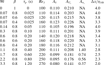
To study the effects of the polymers in the classical statistics of the jet at the far field, a set of 13 spatial direct numerical simulations were carried out. The simulations comprise 12 DNS of turbulent viscoelastic jets and a reference Newtonian simulation. Table 1 summarises the physical and computational parameters used in the simulations.
Physical and computational parameters of the DNS: global/inlet Weissenberg number ( $Wi=\unicode[STIX]{x1D70F}_{p}(U_{J}-U_{\infty }^{in})/h$); solvent viscosity ratio (
 $\unicode[STIX]{x1D6FD}=\unicode[STIX]{x1D708}^{[s]}/(\unicode[STIX]{x1D708}^{[p]}+\unicode[STIX]{x1D708}^{[s]})$); polymer relaxation time (
 $\unicode[STIX]{x1D70F}_{p}$); averaged Taylor Reynolds number in the far field (
 $Re_{\unicode[STIX]{x1D706}}$); spreading rate constant
 $A_{\unicode[STIX]{x1D6FF}}$; centreline velocity decay rate
 $A_{U_{c}}$; polymer stress decay constant
 $A_{\unicode[STIX]{x1D70E}_{c}}$; mesh resolution (normalised by the Kolmogorov length scale at the jet centreline) at
 $x/h=14$ (
 $\unicode[STIX]{x0394}x/\unicode[STIX]{x1D702}_{14h}$).

All the simulations use the same grid and the same size of the computational domain, with a total of  $N_{x}=512$,
 $N_{y}=512$ and
 $N_{z}=128$ grid points in the streamwise (
 $x$), normal (
 $y$) and spanwise (
 $z$) directions, respectively, and the computational domain (normalised by the inlet slot width
 $h$) in the three directions extends to
 $L_{x}/h=L_{y}/h=18$ and
 $L_{z}/h=4.5$. For the inflow condition, the instantaneous streamwise velocity (
 $u(x,y,z,t)$) is prescribed at the inlet for each time step, while the mean normal and spanwise velocities are set to zero
 $\bar{v}(x=0,y)=\bar{w}(x=0,y)=0$, where an over-bar stands for a statistical mean made along the homogeneous direction
 $z$, combined with a temporal average. The mean inlet velocity
 $\bar{u}(x=0,y)$ is based on a hyperbolic–tangent profile (da Silva & Métais Reference da Silva and Métais2002; Stanley et al. Reference Stanley, Sarkar and Mellado2002; da Silva et al. Reference da Silva, Lopes and Raman2015),
 $$\begin{eqnarray}\bar{u}(x=0,y)=\frac{U_{J}+U_{\infty }^{in}}{2}+\frac{U_{J}-U_{\infty }^{in}}{2}\tanh \left[\frac{h}{4\unicode[STIX]{x1D703}}\left(1-\frac{2|y|}{h}\right)\right],\end{eqnarray}$$
where  $U_{J}=\overline{u}(x=0,y=0)$ is the maximum mean streamwise velocity,
 $U_{\infty }^{in}=\overline{u}(x=0,y=L_{y}/2)$ is a small co-flow velocity and
 $\unicode[STIX]{x1D703}$ is the momentum thickness of the initial shear layer. Notice that (2.14) has to be mirrored about the plane
 $(x,z)$ in order to obtain the desired jet top-hat profile. In all simulations the ratio between the inlet slot width and momentum thickness was set to
 $h/\unicode[STIX]{x1D703}=30$ and random perturbations were prescribed for all velocity components at the inlet. As detailed in e.g. da Silva et al. (Reference da Silva, Lopes and Raman2015), these inlet velocity fluctuations are only imposed within the shear-layer region through a proper convolution function, and are prescribed with an energy spectrum providing an energy input concentrated at the small scales of motion. A relatively high amplitude noise, with a maximum instantaneous amplitude of the turbulent velocity fluctuations set to
 $u^{\prime }(x,y,z,t)/U_{J}=0.1$, was prescribed for all velocity fluctuations at the inlet. As discussed in Stanley et al. (Reference Stanley, Sarkar and Mellado2002), da Silva & Métais (Reference da Silva and Métais2002), da Silva et al. (Reference da Silva, Lopes and Raman2015) and references therein, this amplitude merely speeds up the transition to turbulence, without affecting the far-field fully developed region of the flow. The value of the inlet Reynolds number, defined by,
 $$\begin{eqnarray}Re_{h}=\frac{(U_{J}-U_{\infty }^{in})h}{\unicode[STIX]{x1D708}^{[s]}},\end{eqnarray}$$
was set to  $Re_{h}=3500$ for all the simulations (the ratio between the maximum and co-flow velocities at the jet inlet was set to
 $U_{\infty }^{in}/(U_{J}-U_{\infty }^{in})=0.091$).
As shown in da Silva & Métais (Reference da Silva and Métais2002), Stanley et al. (Reference Stanley, Sarkar and Mellado2002) and references therein, this small co-flow does not affect the turbulent jet statistics, since the lateral boundaries of the computational domain are sufficiently far away from the jet centre plane. Here, we adopt a procedure that allows one to compare the present statistics (jet with co-flow) with data obtained in experimental free jets (see da Silva & Métais (Reference da Silva and Métais2002) and references therein). This procedure is valid provided the co-flow does not affect the jet statistics, which is the case here since  $U_{\infty }/U_{J}<0.1$ (Youssef Reference Youssef2012), and consists in computing the streamwise velocity (and related statistics) in a reference frame moving with the co-flow velocity e.g. the initial jet velocity
 $U_{J}$ is actually
 $U_{J}-U_{\infty }^{in}$. Likewise, the centreline mean velocity is subtracted from the local co-flow velocity, i.e.
 $U_{c}(x)$ is actually,
 $U_{c}(x)-\overline{u}(\!x,y=L_{y}/2$. For clarity, in the subsequent text of the paper (and figures), this change of reference frame is not explicitly indicated.
A local turbulence Reynolds number based on the Taylor micro-scale  $\unicode[STIX]{x1D706}$, is defined as,
 $$\begin{eqnarray}Re_{\unicode[STIX]{x1D706}}=\frac{\sqrt{\overline{u^{\prime 2}}}\unicode[STIX]{x1D706}}{\unicode[STIX]{x1D708}^{[s]}},\end{eqnarray}$$
where  $\sqrt{\overline{u^{\prime 2}}}$ is the root-mean square of the streamwise velocity component, and
 $\unicode[STIX]{x1D706}$ is calculated from the classical isotropic relation,
 $$\begin{eqnarray}\unicode[STIX]{x1D706}=\sqrt{\frac{15\unicode[STIX]{x1D708}^{[s]}\overline{u^{\prime 2}}}{\unicode[STIX]{x1D700}^{[s]}}},\end{eqnarray}$$
with the mean viscous dissipation rate of the solvent given by,
 $$\begin{eqnarray}\unicode[STIX]{x1D700}^{[s]}=2\unicode[STIX]{x1D708}^{[s]}\overline{\unicode[STIX]{x1D61A}_{ij}^{\prime }\unicode[STIX]{x1D61A}_{ij}^{\prime }},\end{eqnarray}$$
where  $\unicode[STIX]{x1D61A}_{ij}^{\prime }=(\unicode[STIX]{x2202}u_{i}^{\prime }/\unicode[STIX]{x2202}x_{j}+\unicode[STIX]{x2202}u_{j}^{\prime }/\unicode[STIX]{x2202}x_{i})/2$ is the fluctuating rate-of-strain tensor.
The values of  $Re_{\unicode[STIX]{x1D706}}$ shown in table 1 were computed at the jet centreline by averaging the local
 $Re_{\unicode[STIX]{x1D706}}$ in the streamwise direction in the far-field region (
 $x/h\geqslant 10$). The Kolmogorov length scale, used in table 1 to quantify the resolution of the simulations, is defined by
 $$\begin{eqnarray}\unicode[STIX]{x1D702}=\left(\frac{\unicode[STIX]{x1D708}^{[s]^{3}}}{\unicode[STIX]{x1D700}^{[s]}}\right)^{1/4}.\end{eqnarray}$$
The viscoelastic simulations essentially differ in the value of the maximum relaxation time of the polymer molecules  $\unicode[STIX]{x1D70F}_{p}$, and in the ratio between the solvent and total viscosity of the solution
 $\unicode[STIX]{x1D6FD}=\unicode[STIX]{x1D708}^{[s]}/(\unicode[STIX]{x1D708}^{[s]}+\unicode[STIX]{x1D708}^{[p]})$, while the maximum extensibility length of the polymer molecules
 $L^{2}=100^{2}$ is kept unchanged. The chosen values for
 $L^{2}$,
 $\unicode[STIX]{x1D70F}_{p}$ and
 $\unicode[STIX]{x1D6FD}$ are similar to those used in simulations of homogeneous isotropic turbulence performed in the literature (see Valente, da Silva & Pinho (Reference Valente, da Silva and Pinho2014), Ferreira, da Silva & Pinho (Reference Ferreira, da Silva and Pinho2016) and references therein) and correspond approximately to the values used in recent experimental works of homogeneous isotropic turbulence with polyacrylamide with different weight concentrations (Ouellette, Xu & Bodenschatz Reference Ouellette, Xu and Bodenschatz2009; Xi, Bodenschatz & Xu Reference Xi, Bodenschatz and Xu2013).
Finally, to characterise the flow we define a global (or inlet) Weissenberg number,
 $$\begin{eqnarray}Wi=\frac{\unicode[STIX]{x1D70F}_{p}}{h/(U_{J}-U_{\infty }^{in})},\end{eqnarray}$$
and also a local Weissenberg number,
 $$\begin{eqnarray}Wi_{\unicode[STIX]{x1D702}}=\frac{\unicode[STIX]{x1D70F}_{p}}{\unicode[STIX]{x1D70F}_{\unicode[STIX]{x1D702}}},\end{eqnarray}$$
by comparing the maximum relaxation time of the polymer molecules and the characteristic time scale of the small dissipative scales, given by the Kolmogorov time scale  $\unicode[STIX]{x1D70F}_{\unicode[STIX]{x1D702}}=(\unicode[STIX]{x1D708}^{[s]}/\unicode[STIX]{x1D700}^{[s]})^{1/2}$. The Deborah number
 $De$ can be seen as the counterpart of the Weissenberg number, where the characteristic time scale of the flow is associated with the large scales. This Deborah number is defined here as,
 $$\begin{eqnarray}De=\frac{\unicode[STIX]{x1D70F}_{p}}{t_{c}},\end{eqnarray}$$
where  $t_{c}=\unicode[STIX]{x1D6FF}(x)/U_{c}(x)$ is a convective time scale characteristic of the large energy-carrying eddies.
2.4 Validation
As described in § 2.2 the present code is based on the algorithm described in da Silva & Métais (Reference da Silva and Métais2002) and da Silva et al. (Reference da Silva, Lopes and Raman2015), to which the FENE-P model equations have been added.
For the Newtonian case the present code was extensively validated in da Silva et al. (Reference da Silva, Lopes and Raman2015) throughout comparisons of flow statistics with experimental and numerical data available in the literature. It is based on a version of the code previously described in da Silva & Métais (Reference da Silva and Métais2002) that had also been extensively validated in that paper (and references therein). The new reference Newtonian DNS carried out here was validated by comparing its statistical results with data from these two previous works.
For the viscoelastic cases, however, it is not possible to perform statistical comparisons with experimental data since experimental results for the present flow conditions are not available, and in addition, for other flow conditions the rheology of the fluids used is not adequately characterised. Indeed, the few experimental works of turbulent viscoelastic jets were carried out for circular jets, and even in these cases, the corresponding FENE-P model parameters cannot be estimated from the information described in the literature. Nevertheless, the implementation of the numerical algorithm for the FENE-P model equations in the present code has been verified and validated following the same procedure used previously by the authors for other similar codes e.g. Valente et al. (Reference Valente, da Silva and Pinho2014) and Ferreira et al. (Reference Ferreira, da Silva and Pinho2016), for isotropic turbulence, by making detailed comparisons with several solutions, such as laminar Couette flow (Pimentel Reference Pimentel2019), and laminar planar jet flow (Parvar, da Silva & Pinho Reference Parvar, da Silva and Pinho2020a,Reference Parvar, da Silva and Pinhob), for which the FENE-P model has analytical solutions.
Due to the accuracy and robustness of the present numerical methods and code, and the extensive validations carried out, the present DNS of turbulent viscoelastic planar jets can be seen as the first reference data for this particular flow configuration.
3 Turbulence characteristics of viscoelastic planar jets
This section describes the characteristics of viscoelastic planar jets by comparing these with the statistics obtained in the Newtonian reference simulation.
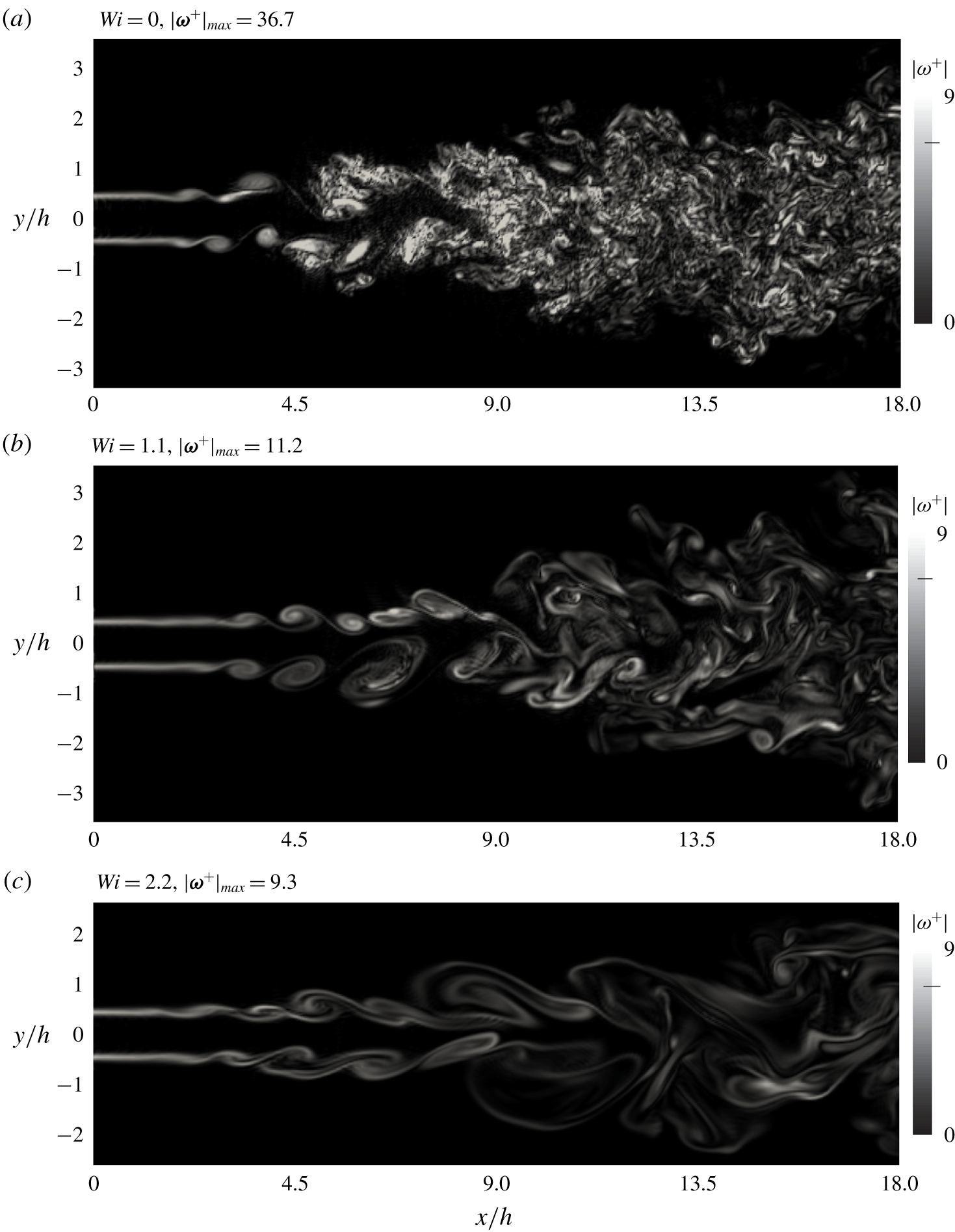
Contours of vorticity magnitude normalised by  $(U_{J}-U_{\infty }^{in})/h$ in the mid-plane (
 $z=0$) of the computational domain for turbulent jets with different Weissenberg numbers. Notice that the figures do not show the total extent of the computational domain used in the lateral (
 $y$) dimension.

3.1 Contours of instantaneous vorticity magnitude and trace of the conformation tensor
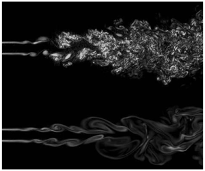
Figure 1 shows two-dimensional contours of instantaneous vorticity magnitude normalised by the mean shear rate at the inlet ( $|\unicode[STIX]{x1D74E}^{+}|=|\unicode[STIX]{x1D74E}|h/(U_{J}-U_{\infty }^{in})$) for three flows with different values of the (global) Weissenberg number,
 $Wi$, in particular for
 $Wi=0$ (Newtonian),
 $Wi=1.1$ and
 $Wi=2.2$. The reference Newtonian case (figure 1a) shows the typical features of the vorticity structures observed in turbulent (Newtonian) jets, with the emergence of initial Kelvin–Helmholtz vortices and their merging into secondary structures (
 $1.8\lesssim x/h\lesssim 3.6$), the strong interaction between the upper and lower shear layers (
 $4.0\lesssim x/h\lesssim 7.8$) and the intense small-scale eddies characteristic of the fully developed turbulent region (
 $9\lesssim x/h\lesssim 18$). As the value of
 $Wi$ increases we observe three main differences, compared with the Newtonian reference case: (i) a considerable depletion of small-scale vorticity throughout the flow field, observed by a decrease in the values of
 $|\unicode[STIX]{x1D74E}^{+}|$, (ii) a tendency for the eddy structures to become much more elongated and (iii) a smaller jet spreading. These observations agree with the experimental visualisation studies performed by several authors (see § 1).
The effect of viscoelasticity on the eddy structure of turbulent viscoelastic flows has been described and studied in numerous studies and in a variety of turbulent flows e.g. Sureshkumar, Beris & Handler (Reference Sureshkumar, Beris and Handler1997), Perlekar, Mitra & Pandit (Reference Perlekar, Mitra and Pandit2006, Reference Perlekar, Mitra and Pandit2010), Horiuti, Matsumoto & Fujiwara (Reference Horiuti, Matsumoto and Fujiwara2013) and Graham (Reference Graham2014). In particular, the reduction in the values of vorticity, as observed in the decrease of  $|\unicode[STIX]{x1D74E}^{+}|$, can be explained from the transport equation of vorticity where the contribution from the polymer appears as a counter torque which results in the suppression of the generation of vortices (Kim et al. Reference Kim, Li, Sureshkumar, Balachandar and Adrian2007; Horiuti et al. Reference Horiuti, Matsumoto and Fujiwara2013). Furthermore, the drastic increase in elongational viscosity increases the resistance of the vortices, and the vortex stretching is diminished (although the fluid is shear thinning, the decrease in shear viscosity is negligible compared to the increase in elongational viscosity).
The smaller jet spreading can be linked to the decrease of the small-scale vorticity, and thus to the decrease of the viscous dissipation rate (discussed below). Since the entrainment in a jet is mainly caused by small-scale ‘nibbling’ associated with the small-scale vortices, rather than large-scale ‘engulfment’ (da Silva et al. Reference da Silva, Hunt, Eames and Westerweel2014), when small vortices are ‘suppressed’ it is expected that the jet will spread at a slower rate.
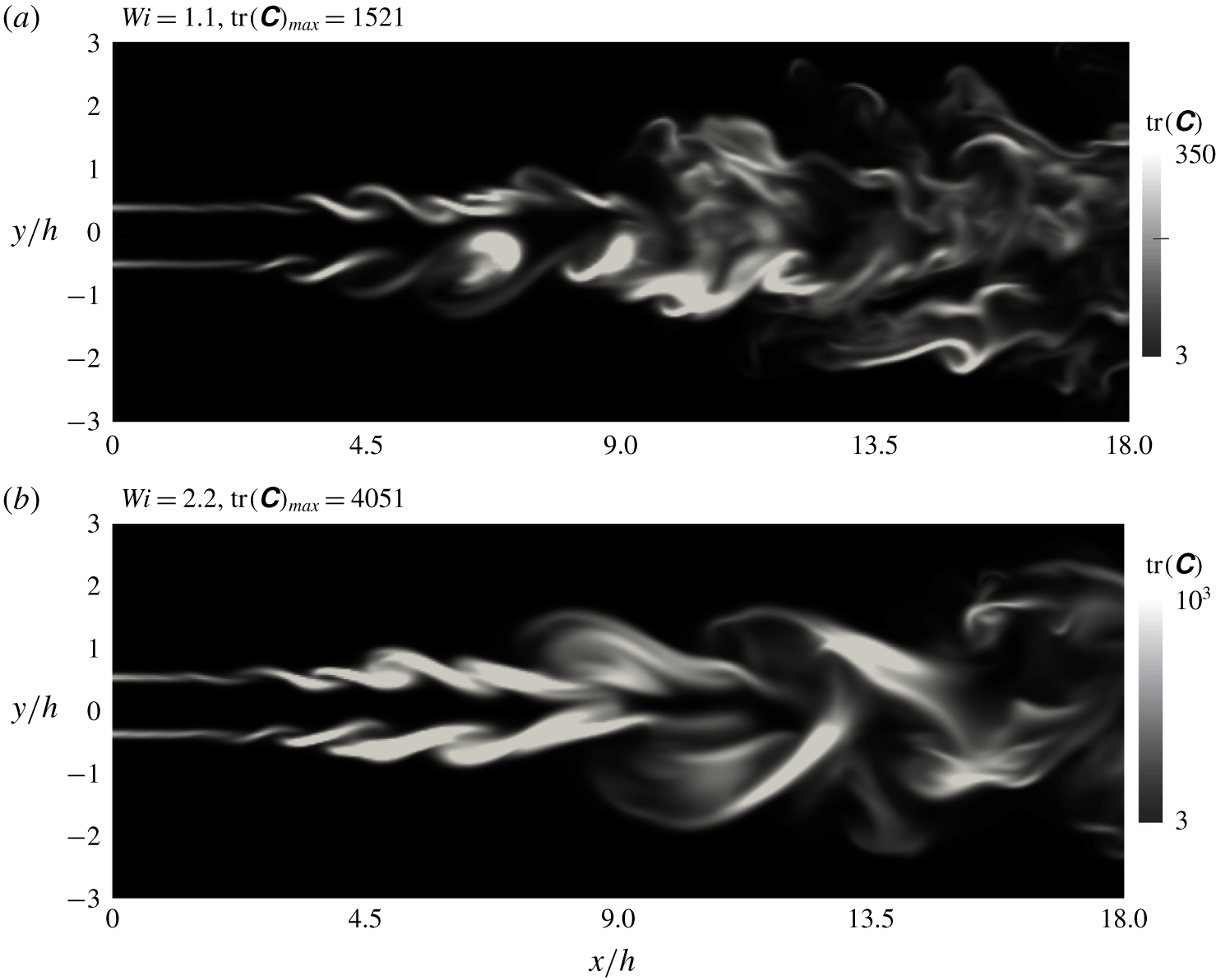
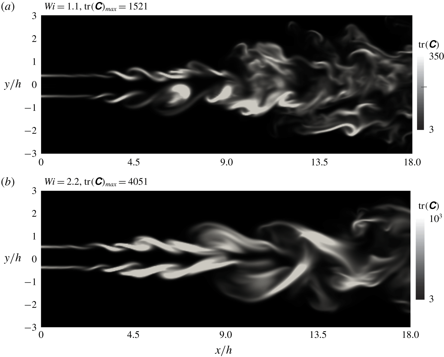
Figure 2(a,b) shows contours of the trace of the conformation tensor  $\text{tr}(\unicode[STIX]{x1D63E})$, which by definition is the root-mean-squared elongation of the polymer chains, for the cases
 $Wi=1.1$ and
 $Wi=2.2$, for the same instants, and in the same
 $(x,y)$ planes, depicted in figures 1(b) and 1(c), respectively. Notice that we use a colour map range with a maximum which is considerably lower than the actual value of
 $\text{max}(\text{tr}(\unicode[STIX]{x1D63E}))$, in order to properly visualise the field at the far-field region of the flow, because
 $\text{tr}(\unicode[STIX]{x1D63E})$ rapidly decays in the streamwise direction.
The values of  $\text{tr}(\unicode[STIX]{x1D63E})$ at the far-field region can become as large as
 $O(350)$, for the case with
 $Wi=1.1$, and
 $O(1000)$, for the case with
 $Wi=2.2$, and are even larger at the transitional region of the flow. By visual inspection it is clear that
 $\text{tr}(\unicode[STIX]{x1D63E})$ is not strongly correlated with the vorticity magnitude in the flow. Whereas the vorticity magnitude tends to be concentrated in the large-scale vortex tubes that emerge during the transition, the most intense values of
 $\text{tr}(\unicode[STIX]{x1D63E})$ are mostly concentrated in the regions between the vortices, where typically the most intense values of strain are located. This is consistent with the fact that the FENE-P model assumes a complete affinity of the motion of the dumbbells to the macroscopic deformation imposed by the flow field. Thus, it is expected that
 $\text{tr}(\unicode[STIX]{x1D63E})$ will be larger at regions with both intense deformation and weak rotation. One such region is the initial shear layer (
 $x/h<2$) where both strain and vorticity have a maximum but where no vortices have yet formed.
The maximum value of  $\text{tr}(\unicode[STIX]{x1D63E})$ obtained for these instantaneous fields corresponds to the simulation with
 $Wi=2.2$ where we have
 $\text{tr}(\unicode[STIX]{x1D63E})_{max}\approx 1000$ in the fully developed turbulence region (
 $x/h>14$). This corresponds to
 $\text{tr}(\unicode[STIX]{x1D63E})_{max}/L^{2}\approx 0.1$, however, a detailed inspection of the instantaneous fields shows that these values are extremely rare, and that only a very small fraction of flow points display these values of
 $\text{tr}(\unicode[STIX]{x1D63E})/L^{2}$. For the large majority of flow points
 $\text{tr}(\unicode[STIX]{x1D63E})/L^{2}\ll 1$. The same result was observed in Valente et al. (Reference Valente, da Silva and Pinho2014), where a similar numerical scheme has been used, and where much higher values of the Weissenberg number have been simulated. Thus, we conclude that, as in Valente et al. (Reference Valente, da Silva and Pinho2014), the condition
 $\text{tr}(\unicode[STIX]{x1D63E})/L^{2}\ll 1$ is also observed here, which validates the use of the FENE-P rheological model in the present simulations, since the polymer molecules are not too stretched, and their lengths remain small compared to their maximum extensibility length.


3.2 Classical statistics
This section analyses the influence of the Weissenberg number on the classical one-point statistics of the velocity and conformation tensor fields. For clarity, only four cases are considered  $Wi=0$ (Newtonian), and
 $Wi=1.1$, 2.2 and 3.3.
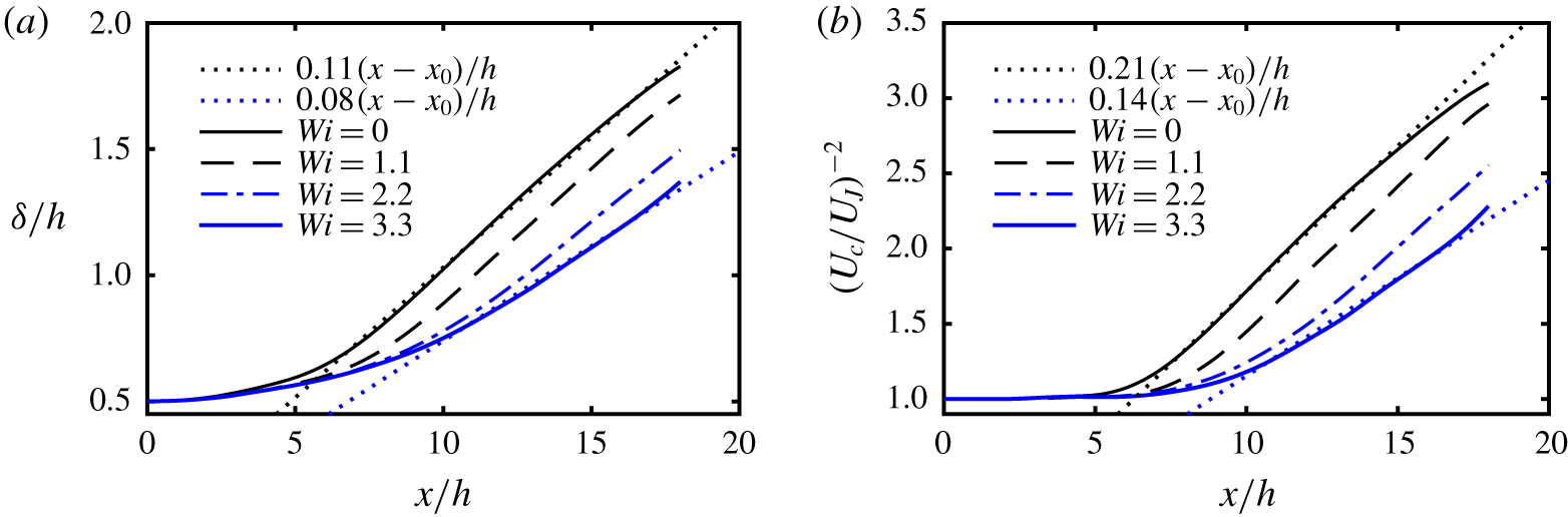
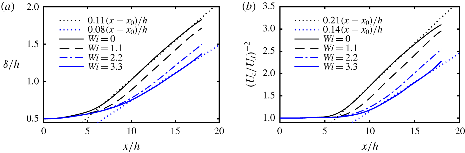
We start with the evolution of the turbulent statistics along the centreline. Figures 3(a) and 3(b) show the streamwise evolution of the shear-layer thickness  $\unicode[STIX]{x1D6FF}(x)$ and the centreline velocity
 $U_{c}(x)$, respectively (appendix A discusses the particular definition of
 $\unicode[STIX]{x1D6FF}(x)$ used in the present work). In all cases, provided the streamwise coordinate
 $x$ is above a given threshold of approximately
 $x/h\gtrsim 7-10$, consistent with the existence of a self-similar, fully developed regime, the shear-layer thickness is a linear function of
 $x$ i.e.
 $$\begin{eqnarray}\frac{\unicode[STIX]{x1D6FF}(x)}{h}=A_{\unicode[STIX]{x1D6FF}}\left(\frac{x-x_{0}}{h}\right),\end{eqnarray}$$
where  $A_{\unicode[STIX]{x1D6FF}}$ is a constant and
 $x_{0}$ is the virtual origin of the jet (see figure 3a). This power law is well known for the case of the Newtonian turbulent planar jet but has rarely been observed in a systematic way for turbulent planar jets of viscoelastic fluids.
The value of  $A_{\unicode[STIX]{x1D6FF}}\approx 0.110$ obtained here for the Newtonian jet is well within the range of values of
 $0.092\leqslant A_{\unicode[STIX]{x1D6FF}}\leqslant 0.118$ observed in many previous experimental (Gutmark & Wygnansky Reference Gutmark and Wygnansky1976; Browne et al. Reference Browne, Antonia, Rajagopalan, Chambers, Dumas and Fulachier1982; Ramaprian & Chandrasekhara Reference Ramaprian and Chandrasekhara1985; Thomas & Chu Reference Thomas and Chu1989; Thomas & Prakash Reference Thomas and Prakash1991; Deo, Mi & Nathan Reference Deo, Mi and Nathan2008; Deo, Nathan & Mi Reference Deo, Nathan and Mi2013)) and numerical (da Silva & Métais Reference da Silva and Métais2002; Stanley et al. Reference Stanley, Sarkar and Mellado2002; da Silva et al. Reference da Silva, Lopes and Raman2015) works. Table 1 shows the values of
 $A_{\unicode[STIX]{x1D6FF}}$ for all the simulations used in the present work, computed between
 $8.5\leqslant x/h\leqslant 17$.
Clearly the Weissenberg number has an effect on the jet spreading. When the  $Wi$ number increases initially to
 $Wi=1.1$ the transition from the potential core to the fully developed state seems to take longer, but otherwise a similar spreading rate (as in the Newtonian case) is recovered (compare
 $\unicode[STIX]{x1D6FF}(x)$ for
 $Wi=0$ and
 $Wi=1.1$). However, when the Weissenberg number increases further to
 $Wi=1.7$, 2.2 and 3.3, even though a linear scaling law is still recovered (
 $\unicode[STIX]{x1D6FF}(x)\sim x$) the spreading rate, assessed through the constant
 $A_{\unicode[STIX]{x1D6FF}}$, is greatly reduced compared with a Newtonian jet i.e.
 $A_{\unicode[STIX]{x1D6FF}}=0.099$, 0.095 and 0.080 for
 $Wi=1.7$, 2.2 and 3.3, respectively, compared to
 $A_{\unicode[STIX]{x1D6FF}}=0.110$ for the Newtonian jet. This also confirms the visual picture formed when analysing the vorticity magnitude fields in figure 1.
Streamwise evolution of the shear-layer thickness  $\unicode[STIX]{x1D6FF}(x)$ normalised by the inlet slot width of the jet
 $h$ (a), and of the centreline velocity
 $U_{c}(x)$ normalised by the initial mean velocity
 $U_{J}$ (b), for different Weissenberg numbers
 $Wi=1.1$, 2.2 and 3.3 (
 $Wi=0$ is the reference Newtonian simulation). The dotted lines are straight lines fit to the cases
 $Wi=0$ (Newtonian) and
 $Wi=3.3$.
Similarly, for all the simulations the centreline velocity variation exhibits the same decay law as in the Newtonian planar jet
 $$\begin{eqnarray}\left(\frac{U_{c}(x)}{U_{J}}\right)^{-2}=A_{U_{c}}\left(\frac{x-x_{0}}{h}\right),\end{eqnarray}$$
where  $A_{U_{c}}$ is a constant, and
 $U_{J}$ is the initial jet velocity. Table 1 shows the values of
 $A_{U_{c}}$ for all the simulations used in the present work, computed between
 $8.5\leqslant x/h\leqslant 17$. Again, the value of
 $A_{U_{c}}\approx 0.210$ obtained here for the Newtonian jet is well within the range of values of
 $0.093\leqslant A_{U_{c}}\leqslant 0.220$ observed in many previous experimental (Gutmark & Wygnansky Reference Gutmark and Wygnansky1976; Browne et al. Reference Browne, Antonia, Rajagopalan, Chambers, Dumas and Fulachier1982; Ramaprian & Chandrasekhara Reference Ramaprian and Chandrasekhara1985; Thomas & Chu Reference Thomas and Chu1989; Thomas & Prakash Reference Thomas and Prakash1991; Deo et al. Reference Deo, Mi and Nathan2008, Reference Deo, Nathan and Mi2013) and numerical (da Silva & Métais Reference da Silva and Métais2002; Stanley et al. Reference Stanley, Sarkar and Mellado2002; da Silva et al. Reference da Silva, Lopes and Raman2015) works.
As for the jet width, two situations can be observed when comparing the centreline velocity decay for Newtonian and viscoelastic jets (see figure 3b and table 1). Whereas for  $Wi\lesssim 1.1$ the effect of the polymer molecules is to slow down the transition to turbulence while keeping the spreading rate approximately equal to the case of the Newtonian jet, for higher values of
 $Wi$ (1.7, 2.2 and 3.3) the velocity decay rate is also strongly decreased compared to the Newtonian reference case. This is attested by the values of the decay constant
 $A_{U_{c}}$, which for
 $Wi=1.7$, 2.2 and 3.3 is equal to
 $A_{U_{c}}=0.181$, 0.176 and 0.141, respectively, compared to
 $A_{U_{c}}\approx 0.21$ in the Newtonian and
 $Wi=1.1$ cases. It is well known that the shear-layer spreading is associated with the centreline velocity decay and it is therefore not surprising to observe the existence of a consistent behaviour between the two quantities in the two figures.
The slower spreading rate described above for viscoelastic planar jets is in qualitative agreement with the experimental data of Usui et al. (Reference Usui, Sano, Kawata and Sakai1980), Berman & Tan (Reference Berman and Tan1985) and Koziol & Glowacki (Reference Koziol and Glowacki1989) and the visualisation studies of Gadd (Reference Gadd1965, Reference Gadd1966), White (Reference White and Wells1969), White (Reference White1972), Wu (Reference Wu and Wells1969), Hoyt et al. (Reference Hoyt, Taylor and Runge1974), Shul’Man et al. (Reference Shul’Man, Pokryvailo, Kovalevskaya and Kulebyakin1973), Filipsson et al. (Reference Filipsson, Lagerstedt and Bark1977), Usui et al. (Reference Usui, Sano, Kawata and Sakai1980) and Gyr (Reference Gyr1996), even if these report data from circular viscoelastic jets. The slower rate of centreline velocity decay agrees also with the measurements of Berman & Tan (Reference Berman and Tan1985) and Koziol & Glowacki (Reference Koziol and Glowacki1989).
Streamwise evolution of the root-mean square of velocity components normalised by the centreline mean velocity  $U_{c}(x)$ for different Weissenberg numbers.

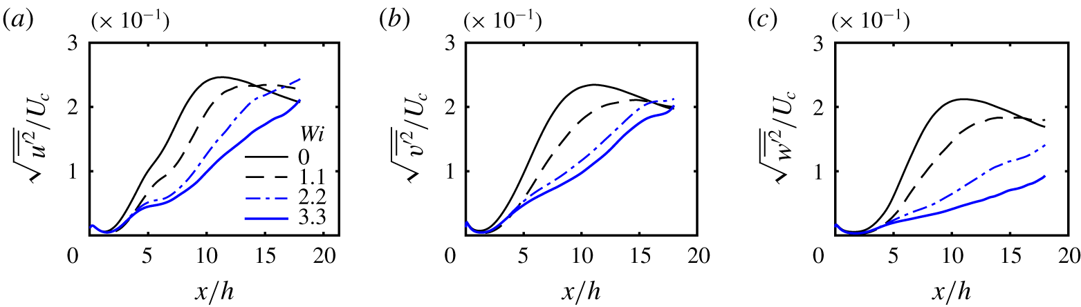
We now turn to the streamwise evolution of the root-mean square of the velocity fluctuations of the jet flow at the centreline as depicted in figure 4(a–c) for the streamwise  $\sqrt{\overline{u^{\prime 2}}}$, normal
 $\sqrt{\overline{v^{\prime 2}}}$ and spanwise
 $\sqrt{\overline{w^{\prime 2}}}$ components, respectively, normalised by the centreline mean velocity
 $U_{c}(x)$. The normal turbulent stresses for the Newtonian case (
 $Wi=0$) show the typical increase associated with the transition to turbulence with saturation located at about
 $x/h\approx 9$, followed by a subsequent decay at a constant rate, a sign of the flow having attained the fully developed turbulent regime. The normal stresses pertaining to the viscoelastic simulation at
 $Wi=1.1$ show basically the same features, although the stresses are slightly smaller compared to the Newtonian case and the peak values are attained slightly later, by
 $x/h\approx 10$. The transition to turbulence for the higher Weissenberg number flows at
 $Wi=2.2$ and 3.3 seems to take place even later, and to be associated with slightly smaller normal stresses. In particular, at
 $x/h=12$, the maximum value of
 $\sqrt{\overline{w^{\prime 2}}}/U_{c}$ for
 $Wi=2.2$ is reduced by a factor of approximately 50 %. For the corresponding transverse and streamwise quantities the reduction is progressively less intense. Consistently with the visualisations of the vorticity magnitude and the spreading rate of the jet, these results show that the effect of the polymers is to decrease the turbulent velocity fluctuations in the far-field region, and to delay the transition to turbulence. These results are also in qualitative agreement with the experimental data of Usui et al. (Reference Usui, Sano, Kawata and Sakai1980).
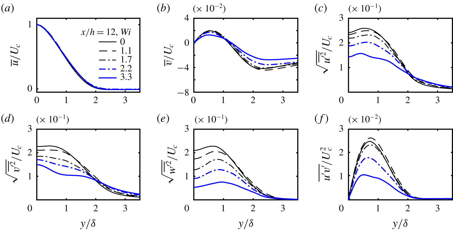
Transverse mean profiles of several turbulent statistics at  $x/h=12$ for the simulations with
 $Wi=0$ (Newtonian),
 $Wi=1.1$, 1.7, 2.2 and 3.3, normalised with the centreline mean velocity
 $U_{c}(x)$ and the thickness of the jet
 $\unicode[STIX]{x1D6FF}(x)$: (a) streamwise mean velocity; (b) normal mean velocity; (c) normal Reynolds stresses in the streamwise direction; (d) normal Reynolds stresses in the normal direction; (e) normal Reynolds stresses in the spanwise direction; (f) Reynolds shear stresses.

The transverse mean profiles of several other turbulence quantities provide more insight into the effects of the polymers on the dynamics of the turbulence. These are displayed in figure 5 for the simulations with  $Wi=0$ (Newtonian),
 $Wi=1.1$, 1.7, 2.2 and 3.3, at the same location (
 $x/h=12$), where the flow has attained a fully developed turbulent state.
Figure 5(a,b) shows the transverse profiles of  $\bar{u}(x,y)/U_{c}(x)$ and
 $\bar{v}(x,y)/U_{c}(x)$ at
 $x/h=12$, for the simulations with
 $Wi=0$ (Newtonian),
 $Wi=1.1$, 1.7, 2.2 and 3.3. Interestingly, whereas the normalised profiles of
 $\bar{u}$ are invariant to the Weissenberg number, the scaled profiles of
 $\bar{v}(x,y)$ slightly decrease with
 $Wi$ (in absolute value). However, a completely different scenario emerges from the observation of the transverse profiles of normal and shear Reynolds stresses, shown in figure 5(c–f). There is a considerable decrease of the peak values of these (normalised) turbulent stresses as the Weissenberg number increases. For instance, the peak values of
 $\sqrt{\overline{w^{\prime 2}}}/U_{c}$ and
 $\overline{u^{\prime }v^{\prime }}/U_{c}^{2}$ are reduced by approximately 50 % for
 $Wi=2.2$, compared to the Newtonian reference case (
 $Wi=0$). Thus, again, one observes that the polymers strongly decrease the turbulence level in the flow, but surprisingly keep the shape of the mean velocity
 $\bar{u}(x,y)/U_{c}(x)$.
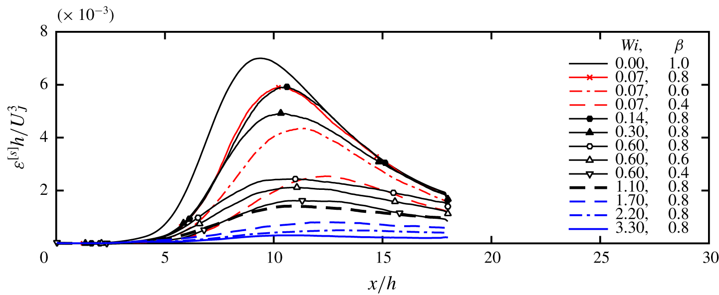
Streamwise evolution of the viscous dissipation rate of turbulent kinetic energy of the solvent  $\unicode[STIX]{x1D700}^{[s]}$, on the centreline, normalised by the initial inlet slot width of the jet
 $h$ and inlet mean velocity
 $U_{J}$.

To complete the characterisation of the turbulent jet, figure 6 shows the streamwise evolution of the normalised viscous dissipation rate of the solvent  $\unicode[STIX]{x1D700}^{[s]}$ for all the simulations carried out in the present work. For all the viscoelastic cases, the dissipation exhibits a similar evolution to the Newtonian reference case, starting with an increase in the transition region followed by a smooth transition downstream of the maximum. The region of slow dissipation decay roughly coincides with the fully developed turbulent region. The fact that the peak dissipation is attained later in the viscoelastic (
 $x/h\gtrsim 10$) than in the Newtonian case (at
 $x/h\approx 9$) also attests to the slower transition to turbulence in those cases. In addition, in all the viscoelastic cases, the dissipation is smaller than in the Newtonian case, and in some cases the difference is quite dramatic.
The smaller solvent dissipation rate in the viscoelastic jets can be explained by the different energy cascade mechanism that is known to exist in viscoelastic turbulence e.g. Valente et al. (Reference Valente, da Silva and Pinho2014). Specifically, since part of the kinetic energy transferred through the classical nonlinear energy cascade is transferred and stored in the polymer molecules, less is present at the small scales, which then leads to a decrease of the small-scale vorticity and viscous dissipation in the solvent. However, for some simulations ( $Wi=0.07,\unicode[STIX]{x1D6FD}=0.8$;
 $Wi=0.14,\unicode[STIX]{x1D6FD}=0.8$;
 $Wi=0.3,\unicode[STIX]{x1D6FD}=0.8$) the dissipation ends by recovering the Newtonian profile for
 $x/h\gtrsim 15$. Thus, for these cases one expects that the polymer molecules do not influence the jet dynamics anymore, since the energy cascade mechanism is apparently not affected. This is confirmed by the values of the spreading rates
 $A_{\unicode[STIX]{x1D6FF}}$ and centreline velocity decay rates
 $A_{U_{c}}$ measured for these simulations, as shown in table 1, that show no significant difference compared to the Newtonian values. The simulations with
 $Wi=0.07$,
 $\unicode[STIX]{x1D6FD}=0.6$ and
 $Wi=0.07$,
 $\unicode[STIX]{x1D6FD}=0.4$ are also interesting because, here, the dissipation value, although smaller than in the Newtonian case, seems to preserve the same Newtonian evolution (local slope) as in the Newtonian case. This is probably because in these cases the polymer effect consists of an additional viscous dissipation, without affecting the energy cascade mechanism. A similar observation was made in isotropic turbulence for low
 $Wi$ numbers, as discussed in Valente, da Silva & Pinho (Reference Valente, da Silva and Pinho2016). Indeed, for the cases with the lowest Weissenberg numbers (
 $Wi=0.07$ and
 $Wi=0.14$) the ratio between the maximum
 $\unicode[STIX]{x1D700}^{[s]}$ observed in the viscoelastic (
 $\unicode[STIX]{x1D700}_{visc.}^{[s]}$) and Newtonian (
 $\unicode[STIX]{x1D700}_{Newt.}^{[s]}$) cases, is approximately equal to the numerical value of the parameter
 $\unicode[STIX]{x1D6FD}$ i.e.
 $\unicode[STIX]{x1D700}_{visc.}^{[s]}/\unicode[STIX]{x1D700}_{Newt.}^{[s]}\approx \unicode[STIX]{x1D6FD}$. This is explained by the weak role played by the elasticity of the fluid at low Weissenberg numbers, whereby a Newtonian behaviour is recovered with total viscosity equal to
 $\unicode[STIX]{x1D708}^{[s]}+\unicode[STIX]{x1D708}^{[p]}=\unicode[STIX]{x1D708}^{[s]}/\unicode[STIX]{x1D6FD}$ (Bird et al. Reference Bird, Curtiss, Armstrong and Hassager1987; Valente et al. Reference Valente, da Silva and Pinho2014). This also explains why
 $\unicode[STIX]{x1D700}^{[s]}$ is approximately equal for the cases with
 $Wi=0.07$,
 $\unicode[STIX]{x1D6FD}=0.8$ and
 $Wi=0.14$,
 $\unicode[STIX]{x1D6FD}=0.8$.
In the remaining cases (including the already discussed simulations with  $Wi=2.2$ and 3.3) not only is the solvent dissipation rate much smaller than in the Newtonian case, the local slope is also very different from the Newtonian case. One expects that in these cases the energy cascade mechanism is strongly affected by the polymers and so is the jet dynamics, which is consistent with the results just discussed. Indeed, for flows at these high Weissenberg numbers, the reduction of
 $\unicode[STIX]{x1D700}^{[s]}$ cannot be simply explained by the viscous effects. In those cases, part of the energy that is not being dissipated by the solvent is transferred to the polymer molecules to be stored as potential elastic energy, or to be dissipated by interactions between the molecules and the strain field of the flow (Valente et al. Reference Valente, da Silva and Pinho2014).
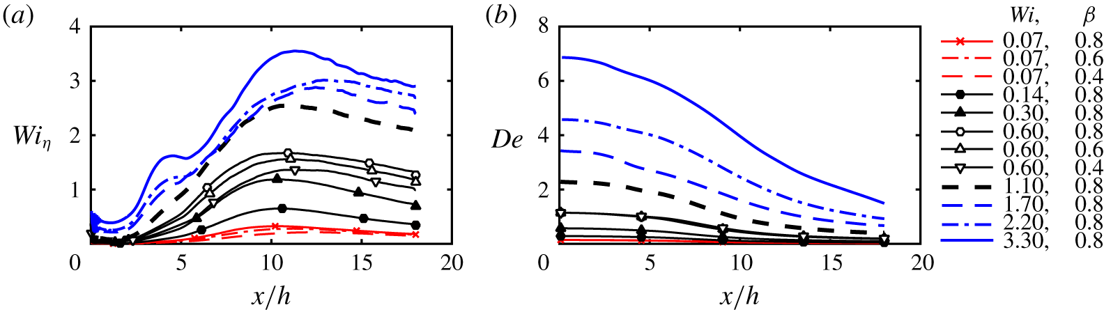
Streamwise evolution of (a) the local Weissenberg number  $Wi_{\unicode[STIX]{x1D702}}=\unicode[STIX]{x1D70F}_{p}/\unicode[STIX]{x1D70F}_{\unicode[STIX]{x1D702}}$ on the centreline, and (b) the local Deborah number
 $De=\unicode[STIX]{x1D70F}_{p}U_{c}/\unicode[STIX]{x1D6FF}$ for all the viscoelastic jet simulations carried in the present work.

The interplay between the polymer molecules and the small dissipative scales of the flow can be appreciated by analysing the streamwise evolution of the local Weissenberg number,  $Wi_{\unicode[STIX]{x1D702}}$ defined in (2.21), as shown in figure 7(a). The curves of
 $Wi_{\unicode[STIX]{x1D702}}$ are similar in shape to the curves of
 $\unicode[STIX]{x1D700}^{[s]}$ discussed above, with an increase in the transition region followed by a slow decrease in the fully developed region, and, for flows with the same
 $\unicode[STIX]{x1D6FD}$, exhibiting a perfect correspondence between the two quantities with the higher local Weissenberg number
 $Wi_{\unicode[STIX]{x1D702}}$ corresponding to smaller solvent viscous dissipation rate
 $\unicode[STIX]{x1D700}^{[s]}$. Three different simulation cases are observed. For
 $Wi=0.07$ and
 $Wi=0.14$ flows the local Weissenberg number is always smaller than
 $Wi_{\unicode[STIX]{x1D702}}<1$. In these cases the energy cascade mechanism taking place in the solvent is not significantly affected by the polymers. For another set of simulations (
 $Wi=0.3,\unicode[STIX]{x1D6FD}=0.8$;
 $Wi=0.6,\unicode[STIX]{x1D6FD}=0.4$) the local Weissenberg number stays momentarily above
 $Wi_{\unicode[STIX]{x1D702}}=1$, for
 $9\lesssim x/h\lesssim 12$ before decreasing to
 $Wi_{\unicode[STIX]{x1D702}}<1$ further downstream at
 $x/h\gtrsim 15$. In these cases, the polymer molecules are expected to affect the flow only momentarily. Finally, in another set of simulations e.g.
 $Wi=1.1$,
 $Wi=1.7$ and
 $Wi=2.2$, and also
 $Wi=0.6,\unicode[STIX]{x1D6FD}=0.8$,
 $Wi=0.6,\unicode[STIX]{x1D6FD}=0.6$, the local Weissenberg number is always
 $Wi_{\unicode[STIX]{x1D702}}>1$ after some station, typically even before the fully developed region is attained (for
 $x/h>12$ for the simulation with
 $Wi=2.2$). Consistently with the previous results, these are the cases where one expects the polymers to have the maximum effect on the solvent dynamics. In particular for the simulation with
 $Wi=3.3$ the local Weissenberg number is close to
 $Wi_{\unicode[STIX]{x1D702}}\approx 3.5$ at some locations, and the polymer molecules are supposedly close to the coil–stretch transition, typically associated with a sharp increase (by a factor of the order of ten thousand) in elongational viscosity (Metzner & Metzner Reference Metzner and Metzner1970; Tirtaatmadja & Sridhar Reference Tirtaatmadja and Sridhar1993; Horiuti et al. Reference Horiuti, Matsumoto and Fujiwara2013). Recall that the local Weissenberg number for this simulation is already within the range of
 $Wi_{\unicode[STIX]{x1D702}}\approx 3{-}4$ where the coil–stretch transition occurs, as strongly suggested in the DNS of isotropic turbulence performed by Watanabe & Gotoh (Reference Watanabe and Gotoh2010).
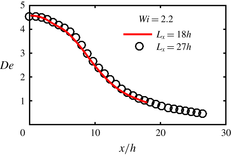
An interesting possibility arises in relation to these figures. Since in all cases the local Weissenberg number exhibits a clear decreasing trend with the increase of the streamwise coordinate, it is likely that the polymer effects on the spatial development of the jets described above, e.g. the decreased spreading rate compared with the Newtonian jet, will cease to be observed very far from the jet origin i.e. when the local streamwise coordinate is  $x/h\gg 1$, even for the most interesting cases described here, such as the simulations with
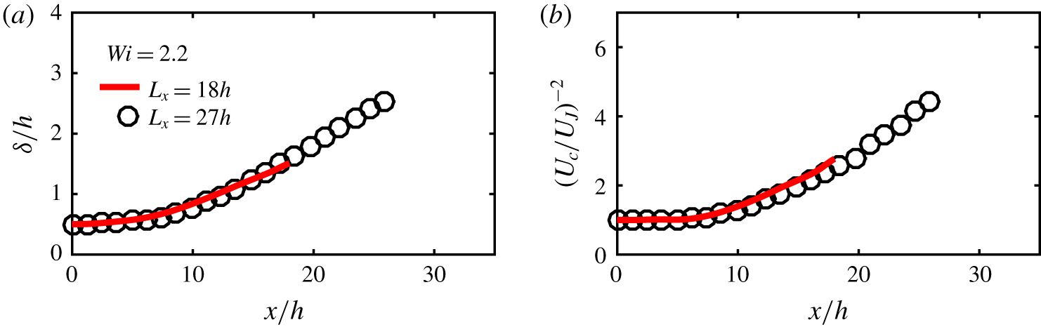
 $Wi=2.2$ and 3.3. This could explain some of the contradictory observations reported in the literature of viscoelastic jets. The investigation of this issue, however interesting, would demand much larger computational domains than are presently possible to simulate, due to the extremely high computational cost of the FENE-P fluid model, and needs to be postponed to a future study. Some preliminary results are discussed in appendix B.
This idea is corroborated in figure 7(b) showing the evolution of the Deborah number  $De$ along the streamwise direction of the jet for all the simulations carried out in this work. At the inlet
 $\unicode[STIX]{x1D6FF}(x=0)=h/2$ by definition (for a top-hat inlet profile), and
 $U_{c}(x=0)=U_{J}$, so that
 $De(x=0)=2Wi$. The Deborah number decreases as the jet streamwise coordinate
 $x$ increases, for all the simulations, but it is above
 $De=1.0$ for at least part of the flow development for many of the simulations, excluding the cases with
 $Wi=0.07$, 0.14, and 0.3. The Deborah number is above
 $De>1.0$ until the end of the domain only for the simulations with
 $Wi=2.2$ and 3.3, and for most of the simulation with
 $Wi=1.7$. This shows that the large scales of the flow are strongly affected by the viscoelastic effects for most of the present simulations, either only during the transition to turbulence and part of the turbulent region (simulations with
 $Wi=0.6$ and 1.1) or during the entire flow development (simulations with
 $Wi>1.7$). Arguably, very far downstream, even in these cases the Deborah number will eventually become much smaller, and the flow will possibly revert to the classical Newtonian dynamics (see appendix B).
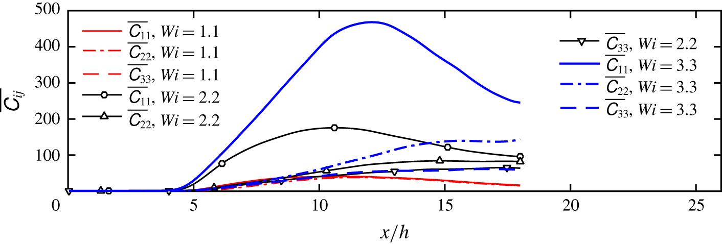
Streamwise evolution of the (mean) diagonal terms of the conformation tensor in the jet centreline, for the simulations with  $Wi=1.1$, 2.2 and 3.3.

To further assess the behaviour of the polymer molecules in the far field of the jet, figure 8 shows the evolution of the (mean) normal components of the conformation tensor  $\overline{\unicode[STIX]{x1D60A}_{ii}}$ (
 $i=1,2,3$, no summation) on the jet centreline, for the simulations with
 $Wi=1.1$, 2.2 and 3.3. Recall that the conformation tensor is normalised by the mean square of the equilibrium radius of the chain
 $\langle R^{2}\rangle _{0}$, so that
 $\unicode[STIX]{x1D60A}_{11}=\unicode[STIX]{x1D60A}_{22}=\unicode[STIX]{x1D60A}_{33}=1.0$ represents the equilibrium (coiled) configuration. Obviously, the polymer molecules are strongly elongated in the three simulation cases (
 $\overline{\unicode[STIX]{x1D60A}_{11}}\gg 1$), and attain their maximum (highest mean elongation) in the range
 $8\lesssim x/h\lesssim 13$, depending on the simulation. The mean values of
 $\overline{\unicode[STIX]{x1D60A}_{ii}}$ are higher for the
 $Wi=3.3$ case than for the other simulations, as expected, but the most interesting aspect here is related to the anisotropy of the conformation tensor. Whereas in the simulation with
 $Wi=1.1$ the conformation tensor is nearly isotropic
 $\overline{\unicode[STIX]{x1D60A}_{11}}=\overline{\unicode[STIX]{x1D60A}_{22}}=\overline{\unicode[STIX]{x1D60A}_{33}}$, except during the transition to turbulence (
 $2\lesssim x/h\lesssim 8$), in the other cases the conformation tensor is not isotropic (
 $\overline{\unicode[STIX]{x1D60A}_{11}}\gg \overline{\unicode[STIX]{x1D60A}_{22}}>\overline{\unicode[STIX]{x1D60A}_{33}}$), although a tendency to isotropy can be observed for
 $Wi=2.2$ (
 $x/h\gtrsim 17$). Figure 8 shows additionally that as the Weissenberg number
 $Wi$ increases,
 $\overline{\unicode[STIX]{x1D60A}_{11}}$ increases at a faster pace than
 $\overline{\unicode[STIX]{x1D60A}_{22}}$ and
 $\overline{\unicode[STIX]{x1D60A}_{33}}$, showing that the polymer chains are more severely stretched and oriented in the streamwise direction of the flow for higher values of
 $Wi$, as expected by the present flow configuration.
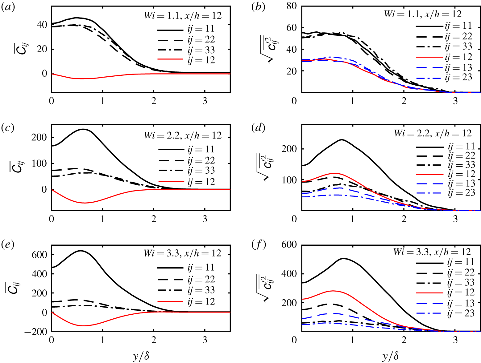
Transverse profiles of mean (a,c,e) and root-mean-squared (r.m.s.) (b,d,f) components of the conformation tensor for flows with different Weissenberg numbers.

This result is confirmed by looking into the transverse profiles of mean and root-mean-squared (r.m.s.) conformation tensor components, for a fixed station ( $x/h=12$) for Weissenberg numbers
 $Wi=1.1$, 2.2 and 3.3 as shown in figure 9(a,c,e) and figure 9(b,d,f), respectively (
 $\unicode[STIX]{x1D624}_{ij}^{\prime }$ is the fluctuation of
 $\unicode[STIX]{x1D60A}_{ij}$ with respect to its mean value i.e.
 $\unicode[STIX]{x1D60A}_{ij}=\overline{\unicode[STIX]{x1D60A}_{ij}}+\unicode[STIX]{x1D624}_{ij}^{\prime }$). Because of the condition of statistical invariance under a reflection of the
 $z$ axis with respect to the
 $(x,y)$ plane, the components
 $\overline{\unicode[STIX]{x1D60A}_{13}}$ and
 $\overline{\unicode[STIX]{x1D60A}_{23}}$ are identically zero everywhere, and thus are not shown in the figures. Again, as the Weissenberg number
 $Wi$ increases, the magnitudes of the mean and r.m.s. values of the conformation tensor components tend to increase, however, interestingly, the components
 $\overline{\unicode[STIX]{x1D60A}_{11}}$ and
 $\overline{\unicode[STIX]{x1D60A}_{12}}$ increase with
 $Wi$ (in absolute values) faster than
 $\overline{\unicode[STIX]{x1D60A}_{22}}$ and
 $\overline{\unicode[STIX]{x1D60A}_{33}}$, thus confirming the enhancement of polymer stretching anisotropy as
 $Wi$ increases and the existence of a preferred stretching of polymers in the streamwise direction of the flow.
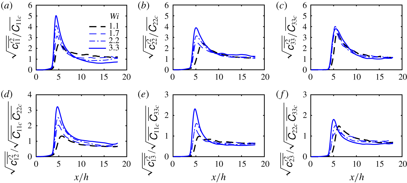
Streamwise evolution (along the centreline) of the root-mean-squared fluctuations of the conformation tensor normal (a–c) and shear (d–f) components normalised by the mean value  $\overline{\unicode[STIX]{x1D60A}_{ij}}_{c}(x)=\overline{\unicode[STIX]{x1D60A}_{ij}}(x,y=0)$ for different Weissenberg numbers.

Although the r.m.s. values of the fluctuations of the conformation tensor increase with the global/inlet Weissenberg number, the turbulent intensities of  $\unicode[STIX]{x1D63E}$ i.e. the fluctuations normalised by the mean values, seem to be independent of
 $Wi$. This is shown in figure 10 for streamwise profiles of
 $\sqrt{\overline{\unicode[STIX]{x1D624}_{ij}^{\prime 2}}}/\sqrt{\overline{\unicode[STIX]{x1D60A}_{ii}}\,\overline{\unicode[STIX]{x1D60A}_{jj}}}$ (no summation) along the jet centreline (
 $y=0$). The evolution of these quantities is characterised by one bump at the transition region followed by a constant plateau of
 $\sqrt{\overline{\unicode[STIX]{x1D624}_{11}^{\prime 2}}}/\overline{\unicode[STIX]{x1D60A}_{11}}\approx \sqrt{\overline{\unicode[STIX]{x1D624}_{22}^{\prime 2}}}/\overline{\unicode[STIX]{x1D60A}_{22}}\approx \sqrt{\overline{\unicode[STIX]{x1D624}_{33}^{\prime 2}}}/\overline{\unicode[STIX]{x1D60A}_{33}}\approx 1$ (normal components) and
 $\sqrt{\overline{\unicode[STIX]{x1D624}_{12}^{\prime 2}}}/\sqrt{\overline{\unicode[STIX]{x1D60A}_{11}}\,\overline{\unicode[STIX]{x1D60A}_{22}}}\approx \sqrt{\overline{\unicode[STIX]{x1D624}_{13}^{\prime 2}}}/\sqrt{\overline{\unicode[STIX]{x1D60A}_{11}}\,\overline{\unicode[STIX]{x1D60A}_{33}}}\approx \sqrt{\overline{\unicode[STIX]{x1D624}_{23}^{\prime 2}}}/\sqrt{\overline{\unicode[STIX]{x1D60A}_{22}}\,\overline{\unicode[STIX]{x1D60A}_{33}}}\approx 0.7$ (shear components), suggesting that the conformation tensor has also attained a fully developed self-similar regime. Notice that these turbulence intensities for the conformation tensor are approximately one order of magnitude higher than the fluctuations of turbulent velocities, which are
 $\sqrt{\overline{u^{\prime 2}}}/U_{c}\approx \sqrt{\overline{v^{\prime 2}}}/U_{c}\approx \sqrt{\overline{w^{\prime 2}}}/U_{c}\approx 0.1$ (see figure 4).
4 Towards a theory for viscoelastic turbulent planar jets
The previous section discussed several features of turbulent viscoelastic planar jets. However, as described in the introduction, no theory of turbulent viscoelastic planar jets presently exists. This section draws from the previous observations, and from the classical analysis methods used to describe Newtonian planar jets, in an attempt to develop a theory for turbulent viscoelastic planar jets. As in the classical theory of the planar jet, we focus on the evolution of the flow field in the fully developed turbulent region, and in this process we adopt the classical assumption that the jet ‘forgets’ the details of its initial (inlet) generation. The fact that viscoelastic jets tend to attain a fully developed regime later than the Newtonian reference simulation (particularly for higher Weissenberg numbers  $Wi$), as discussed above and in agreement with several authors (Berman & Tan Reference Berman and Tan1985), has no relevance to the analysis of the laws governing the far-field, fully developed flow region (even when the fluid has a fading memory, this effect is vanishingly small for sufficiently long time intervals such as those taken by volumes of fluid travelling from the jet inlet up to the far-field region).
We are well aware (and well familiar) with the present ongoing discussion on the validity of the classical theory of jets (and of other flows) as described in several recent references e.g. Sadeghi et al. (Reference Sadeghi, Oberlack and Gauding2018), Layek & Sunita (Reference Layek2018) and Cafiero & Vassilicos (Reference Cafiero and Vassilicos2019). However, it seems that, in the present case, the Newtonian jet recovers the classical scaling laws i.e.  $\unicode[STIX]{x1D6FF}(x)\sim x$ and
 $U_{c}(x)\sim x^{-1/2}$ (see figure 3a,b), compatible with a classical Kolmogorov scaling, and therefore this will be the starting point for the analysis developed here.
4.1 Thin shear-layer approximation for viscoelastic turbulent planar jets
The starting point for the similarity analysis of the mean flow for viscoelastic turbulent planar jets is the thin shear-layer equations, which are given by the momentum equation in the streamwise direction,
 $$\begin{eqnarray}\bar{u}\frac{\unicode[STIX]{x2202}\bar{u}}{\unicode[STIX]{x2202}x}+\bar{v}\frac{\unicode[STIX]{x2202}\bar{u}}{\unicode[STIX]{x2202}y}=-\frac{\unicode[STIX]{x2202}\overline{u^{\prime }v^{\prime }}}{\unicode[STIX]{x2202}y}+\frac{1}{\unicode[STIX]{x1D70C}}\frac{\unicode[STIX]{x2202}\overline{\unicode[STIX]{x1D70E}_{xy}}^{[p]}}{\unicode[STIX]{x2202}y},\end{eqnarray}$$
together with the continuity equation,
 $$\begin{eqnarray}\frac{\unicode[STIX]{x2202}\bar{u}}{\unicode[STIX]{x2202}x}+\frac{\unicode[STIX]{x2202}\bar{v}}{\unicode[STIX]{x2202}y}=0.\end{eqnarray}$$
The momentum equation in the normal ( $y$) direction is treated in the usual way, and explains the absence of the pressure gradient term in (4.1). Implicit in the equations above is the classical assumption that gradients in the normal (
 $y$) direction are much larger than gradients in the streamwise (
 $x$) direction. It is noteworthy that the FENE-P rheological model is not used in the derivation of the present theory.
Solving (4.1) and (4.2) for  $\bar{u}(x,y)$ and
 $\bar{v}(x,y)$ would require closures for the turbulent and polymer stress terms. Usual approximations are the mixing length turbulence model and the FENE-P rheological model. However, a lot of information concerning the evolution of the turbulent flow can still be gained without resorting to those models, as demonstrated in the next sections.
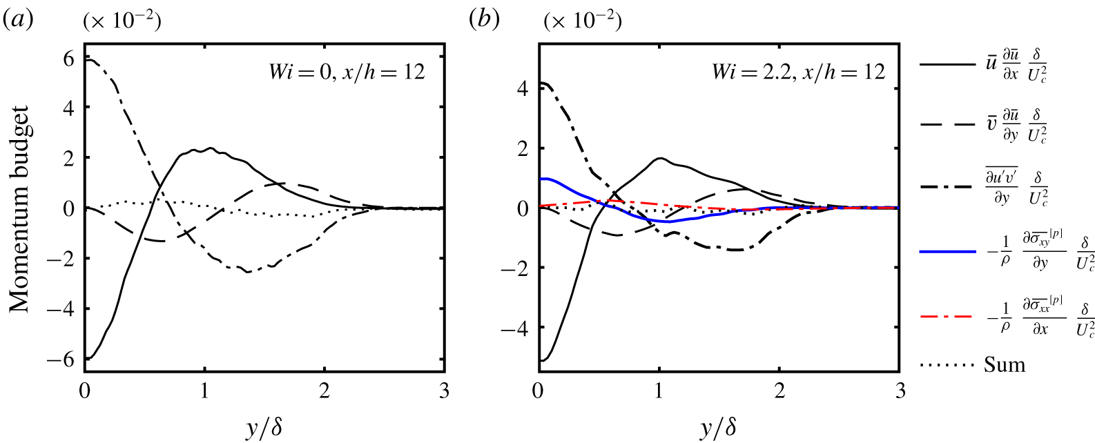
The accuracy of the approximation given by (4.1) can be assessed by comparing the relative order of magnitude of each term in the equation. If the thin shear-layer approximation is exactly verified, all the terms in (4.1) will add up to zero (provided the results are fully converged). These terms are displayed in figure 11 for the Newtonian ( $Wi=0$) and the viscoelastic simulation with
 $Wi=2.2$ at
 $x/h=12$ (the neglected term
 $\unicode[STIX]{x1D70C}^{-1}\unicode[STIX]{x2202}\overline{\unicode[STIX]{x1D70E}_{xx}}^{[p]}/\unicode[STIX]{x2202}x$ is also shown for comparison). The comparison of the relative magnitudes of each term in figure 11 shows that the thin shear-layer approximation, consisting of (4.1)–(4.2), is indeed a very good approximation, considering that, for the Newtonian case, where the turbulent boundary layer approximations are well established, errors can be of the order of 10 % of the dominant term in the equation (Pope Reference Pope2000).
Transverse profiles of the terms from the mean streamwise momentum equation, with the thin shear-layer approximation (4.1), at  $x/h=12$, for the reference Newtonian simulation (a) and for the viscoelastic simulation with
 $Wi=2.2$ (b). The terms are normalised by the centreline mean velocity
 $U_{c}(x)$ and by the thickness of the shear layer
 $\unicode[STIX]{x1D6FF}(x)$, and the dotted lines represent the sum of all the terms shown in the figures except the term
 $-\unicode[STIX]{x1D70C}^{-1}\unicode[STIX]{x2202}\overline{\unicode[STIX]{x1D70E}_{xx}}^{[p]}/\unicode[STIX]{x2202}x$, which is neglected in the thin shear-layer approximation.

4.2 Self-similarity analysis for viscoelastic turbulent planar jets
The classical analysis of the thin shear-layer equations for the turbulent planar jet starts with (4.1) written in conservative form. Integrating this equation in the transverse (or normal  $y$) direction yields,
 $$\begin{eqnarray}\frac{\text{d}}{\text{d}x}\int _{-\infty }^{\infty }\bar{u}^{2}(x,y)\,\text{d}y=0,\end{eqnarray}$$
where the assumptions of (i) zero free-stream turbulence, (ii) zero mean polymer shear stress and (iii) zero mean co-flow velocity in the irrotational region have been used.
In the classical (Newtonian) turbulent jet theory, the hypothesis of self-similarity is introduced at this point, and implies the existence of a reference velocity  $\bar{u_{0}}(x)$, and a length scale
 $\bar{l_{0}}(x)$, with which the normalised profiles of e.g. the mean streamwise velocity
 $\bar{u}(x,y)$, taken from several flow stations
 $x$, all collapse into the same single curve.
Following the usual practice, for velocity and length scales of the flow we chose the centreline velocity  $U_{c}(x)$ and the jet shear-layer thickness
 $\unicode[STIX]{x1D6FF}(x)$,
 $\bar{u_{0}}(x)=U_{c}(x)$ and
 $\bar{l_{0}}(x)=\unicode[STIX]{x1D6FF}(x)$, respectively (the Appendix discusses the particular definition of
 $\unicode[STIX]{x1D6FF}(x)$ used in the present work). Therefore, the normalised streamwise velocity and normal coordinate are,
 $$\begin{eqnarray}\unicode[STIX]{x1D713}=\frac{\bar{u}(x,y)}{U_{c}(x)},\end{eqnarray}$$
and
 $$\begin{eqnarray}\unicode[STIX]{x1D709}=\frac{y}{\unicode[STIX]{x1D6FF}(x)},\end{eqnarray}$$
respectively, so that the self-similarity of the streamwise velocity corresponds to supposing that the function  $\unicode[STIX]{x1D713}=\unicode[STIX]{x1D713}(\unicode[STIX]{x1D709})$ is the same for all the streamwise coordinates
 $x/h$ in a given jet.
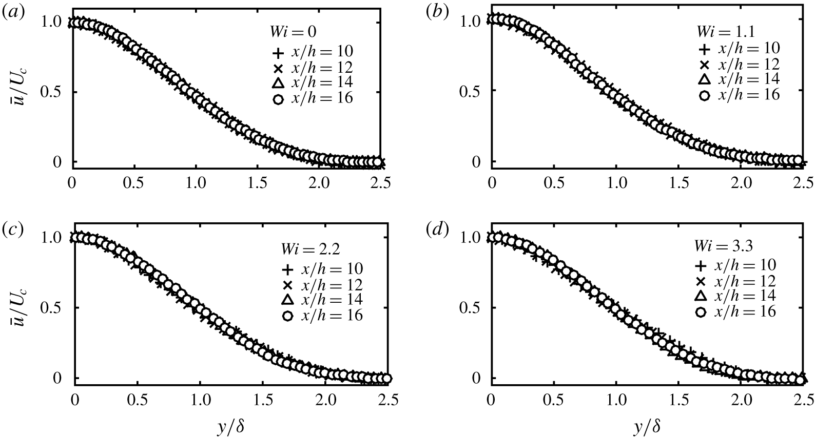
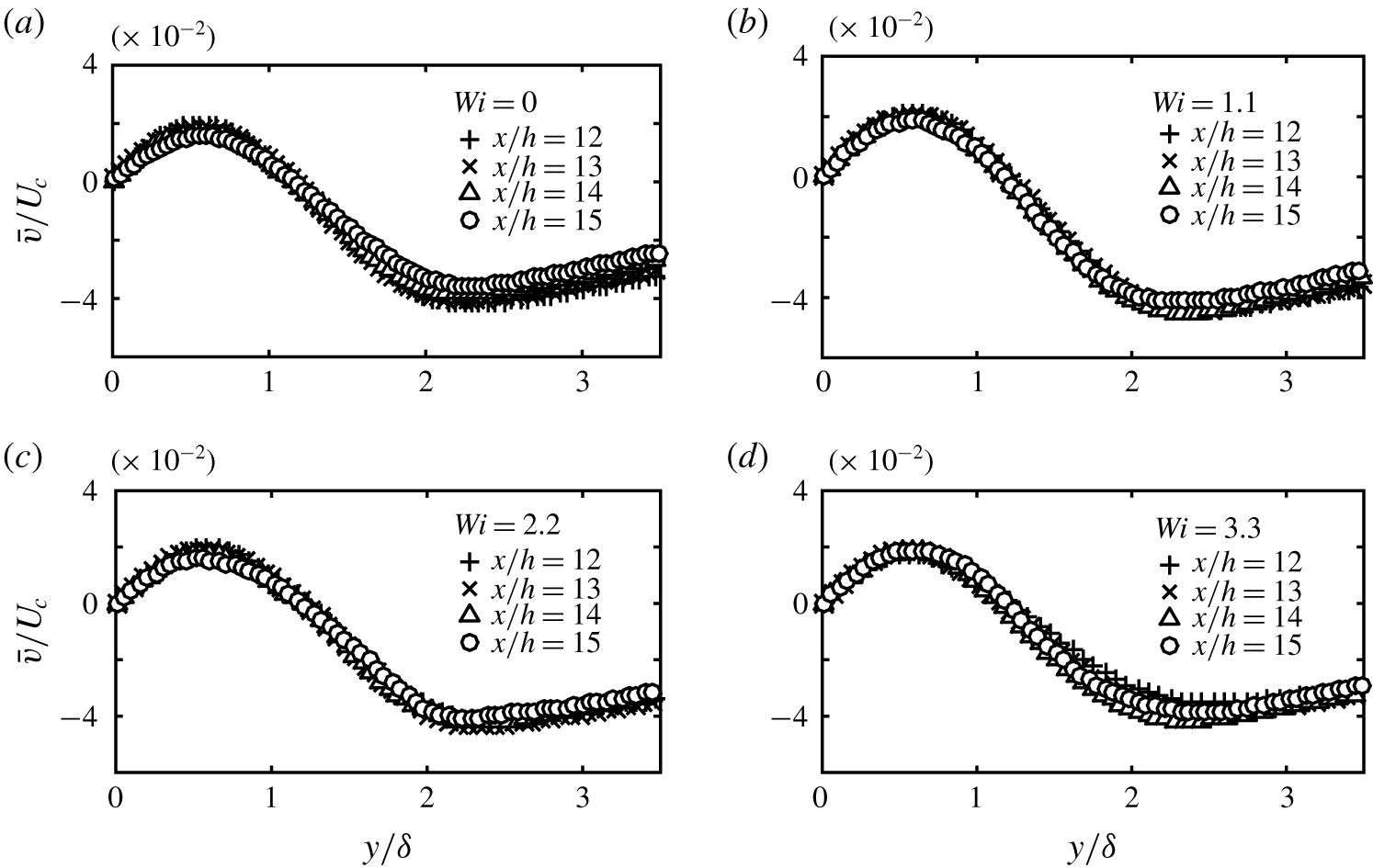
Figures 12(a–d) and 13(a–d) show that self-similarity is indeed recovered for the mean streamwise velocity  $\bar{u}(x,y)$, and also for the normal velocity
 $\bar{v}(x,y)$. These figures show transverse profiles of mean velocities
 $\bar{u}(x,y)$ and
 $\bar{v}(x,y)$ at different stations
 $x/h$, normalised by the jet centreline velocity
 $U_{c}(x)$, and by the jet shear-layer thickness
 $\unicode[STIX]{x1D6FF}(x)$ for the simulations with Newtonian and viscoelastic fluids at Weissenberg numbers
 $Wi=1.1$, 2.2 and 3.3. The collapse of the normalised mean velocities
 $\bar{u}(x,y)/U_{c}(x)$ and
 $\bar{v}(x,y)/U_{c}(x)$ shows that self-similarity is attained at least from
 $x/h=12$ onwards. This is of course no surprise for the Newtonian (
 $Wi=0$) simulation (figures 12a and 13a), but is observed here for the first time for viscoelastic turbulent planar jets. The collapse is apparently less clear for the
 $\bar{v}(x,y)$ velocity due to the very small values of this component which imply slightly less well-converged mean profiles.
Transverse profiles of streamwise mean velocity  $\bar{u}(x,y)$ at several
 $x/h$ stations, normalised by the jet centreline velocity
 $U_{c}(x)$, and jet shear-layer thickness
 $\unicode[STIX]{x1D6FF}(x)$ for the Newtonian and viscoelastic simulations with Weissenberg numbers
 $Wi=1.1$, 2.2 and 3.3.

Transverse profiles of normal mean velocity  $\bar{v}(x,y)$ at several
 $x/h$ stations, normalised by the jet centreline velocity
 $U_{c}(x)$, and jet shear-layer thickness
 $\unicode[STIX]{x1D6FF}(x)$ for the Newtonian and viscoelastic simulations with Weissenberg numbers
 $Wi=1.1$, 2.2 and 3.3.

Inserting the hypothesis of self-similarity for the streamwise mean velocity,
 $$\begin{eqnarray}\bar{u}(x,y)=\unicode[STIX]{x1D713}\left[\frac{y}{\unicode[STIX]{x1D6FF}(x)}\right]U_{c}(x)\end{eqnarray}$$
into (4.3), yields,
 $$\begin{eqnarray}\frac{\text{d}}{\text{d}x}\left[U_{c}^{2}(x)\unicode[STIX]{x1D6FF}(x)\right]=0,\end{eqnarray}$$
which is of course equal to the classical momentum integral constraint observed for a turbulent planar jet of a Newtonian fluid. Self-similarity of the mean streamwise velocity, clearly observed above for the viscoelastic jet (figure 12a–d), naturally implies that the constraint expressed in (4.7) is also valid for turbulent planar jets of viscoelastic fluids.
The classical theory for a Newtonian jet would then continue by assuming self-similarity of the turbulent shear stress profiles  $\overline{u^{\prime }v^{\prime }}(x,y)$, in the sense that, when scaled by
 $U_{c}(x)^{2}$ and
 $\unicode[STIX]{x1D6FF}(x)$, the profiles at several
 $x/h$ stations of the jet will all collapse onto the same curve (Townsend Reference Townsend1976). In the present analysis we do not use this assumption since the presence of the extra polymeric term in (4.1) may preclude this possibility, as there are other (additional) velocity and length scales needed to describe this extra polymeric term, which are not the same ones used for the streamwise
 $\bar{u}(x,y)$ and normal
 $\bar{v}(x,y)$ mean velocity profiles (see § 4.3).
Instead, we simply assume that the same (single) velocity and length scales, namely  $U_{c}(x)$ and
 $\unicode[STIX]{x1D6FF}(x)$, are the relevant quantities needed to characterise the mean profiles of both the streamwise
 $\bar{u}(x,y)$, and the normal
 $\bar{v}(x,y)$ velocity components. Mathematically, this hypothesis assumes that if
 $\unicode[STIX]{x1D713}(\unicode[STIX]{x1D709})=\bar{u}(x,y)/U_{c}(x)$ is a function of
 $\unicode[STIX]{x1D709}=y/\unicode[STIX]{x1D6FF}(x)$ only, so is also
 $\unicode[STIX]{x1D719}(\unicode[STIX]{x1D709})=\bar{v}(x,y)/U_{c}(x)$. This hypothesis agrees with the present data, as discussed above in relation to figures 12 and 13.
From this hypothesis and by using the mean continuity equation we can write,
 $$\begin{eqnarray}\unicode[STIX]{x1D719}(\unicode[STIX]{x1D709})=\frac{\bar{v}(x,y)}{U_{c}(x)}=\frac{\text{d}\unicode[STIX]{x1D6FF}(x)}{\text{d}x}\left\{\unicode[STIX]{x1D713}(\unicode[STIX]{x1D709})\unicode[STIX]{x1D709}-\frac{1}{2}\int _{0}^{\unicode[STIX]{x1D709}}\unicode[STIX]{x1D713}(\tilde{\unicode[STIX]{x1D709}})\,\text{d}\tilde{\unicode[STIX]{x1D709}}\right\}.\end{eqnarray}$$
Since the term inside brackets on the right-hand side of (4.8) is a function of  $\unicode[STIX]{x1D709}$ only, the self-similarity hypothesis for
 $\bar{v}(x,y)$ can only be satisfied if
 $\text{d}\unicode[STIX]{x1D6FF}/\text{d}x$ is constant,
 $$\begin{eqnarray}\unicode[STIX]{x1D6FF}(x)\sim x,\end{eqnarray}$$
and by inserting this result into (4.7) we get the centreline velocity decay law for viscoelastic turbulent jets,
 $$\begin{eqnarray}U_{c}(x)\sim x^{-1/2}.\end{eqnarray}$$
These are exactly the spreading and decay laws described in § 3.2 while discussing the present simulation results for viscoelastic turbulent jets. The fact that these evolution laws are the same as in the Newtonian jet can therefore be simply explained in the same manner for either Newtonian and viscoelastic jets, and stems directly from similar arguments as used in the classical theory of the Newtonian planar jet. Despite this, the scaling constants associated with these laws i.e.  $A_{\unicode[STIX]{x1D6FF}}$ and
 $A_{U_{c}}$ defined in (3.1) and (3.2), are of course very different to the Newtonian values, and are strongly affected by the global Weissenberg number
 $Wi$, as documented above, and as summarised in table 1.
4.3 Similarity laws for the polymer stresses in viscoelastic turbulent planar jets
We now turn to the analysis of the self-similarity and evolution laws of the polymer stresses in turbulent viscoelastic jets.
A question of particular interest for the new theory of the far field of viscoelastic jets developed here is whether there is a region where the transverse profiles of mean polymer shear stress  $\overline{\unicode[STIX]{x1D70E}_{xy}}^{[p]}(x,y)$ become self-preserving, and how does the characteristic scale of these stresses evolve in the streamwise direction
 $x$? If this self-similar region does indeed exist, what is the scaling factor
 $\unicode[STIX]{x1D70E}_{c}^{[p]}(x)$ which will make the profiles of
 $\overline{\unicode[STIX]{x1D70E}_{xy}}^{[p]}(x,y)/\unicode[STIX]{x1D70E}_{c}^{[p]}(x)$ invariant with respect to the distance
 $x$ from the jet orifice? It turns out that these questions can be addressed by using simple phenomenological arguments, as discussed below.
The key problem here is the determination of the speed at which the polymer stresses, at one given location e.g. at the location of maximum shear stress,  $\unicode[STIX]{x1D70E}_{c}^{[p]}(x)=\text{max}|\overline{\unicode[STIX]{x1D70E}_{xy}}^{[p]}(x,y)|$, decay as the flow evolves in the streamwise
 $x$ direction.
The answer to this question can be obtained by analysing the transport equation for the turbulent kinetic energy  $\unicode[STIX]{x1D705}=\overline{\boldsymbol{u}^{\prime }\boldsymbol{\cdot }\boldsymbol{u}^{\prime }}/2$, which is given by,
 $$\begin{eqnarray}\displaystyle \bar{\boldsymbol{u}}\boldsymbol{\cdot }\unicode[STIX]{x1D735}\unicode[STIX]{x1D705} & = & \displaystyle -\frac{1}{\unicode[STIX]{x1D70C}}\unicode[STIX]{x1D735}\boldsymbol{\cdot }\overline{p^{\prime }\boldsymbol{u}^{\prime }}-\frac{1}{2}\unicode[STIX]{x1D735}\boldsymbol{\cdot }\overline{\boldsymbol{u}^{\prime }\boldsymbol{u}^{\prime }\boldsymbol{\cdot }\boldsymbol{u}^{\prime }}+\unicode[STIX]{x1D708}^{[s]}\unicode[STIX]{x1D6FB}^{2}\unicode[STIX]{x1D705}-\overline{\boldsymbol{u}^{\prime }\boldsymbol{u}^{\prime }}\boldsymbol{ : }\unicode[STIX]{x1D735}\overline{\boldsymbol{u}}-\unicode[STIX]{x1D708}^{[s]}\overline{\unicode[STIX]{x1D735}\boldsymbol{u}^{\prime }\boldsymbol{ : }\unicode[STIX]{x1D735}\boldsymbol{u}^{\prime }}\nonumber\\ \displaystyle & & \displaystyle +\,\frac{1}{\unicode[STIX]{x1D70C}}\unicode[STIX]{x1D735}\boldsymbol{\cdot }\overline{{\unicode[STIX]{x1D748}^{\prime }}^{[p]}\boldsymbol{u}^{\prime }}-\frac{1}{\unicode[STIX]{x1D70C}}\overline{{\unicode[STIX]{x1D748}^{\prime }}^{[p]}\boldsymbol{ : }\unicode[STIX]{x1D735}\boldsymbol{u}^{\prime }}.\end{eqnarray}$$
This equation has two terms that explicitly account for the influence of viscoelasticity on the turbulent kinetic energy: the viscoelastic turbulent transport  $\unicode[STIX]{x1D735}\boldsymbol{\cdot }\overline{{\unicode[STIX]{x1D748}^{\prime }}^{[p]}\boldsymbol{u}^{\prime }}/\unicode[STIX]{x1D70C}$ and the viscoelastic stress power
 $\overline{{\unicode[STIX]{x1D748}^{\prime }}^{[p]}\boldsymbol{ : }\unicode[STIX]{x1D735}\boldsymbol{u}^{\prime }}/\unicode[STIX]{x1D70C}$, where
 ${\unicode[STIX]{x1D748}^{\prime }}^{[p]}$ represents fluctuations of the instantaneous polymer stress about its mean value. In the particular case of a flow with a sufficiently high Weissenberg number, it is expected that at least one of these two terms will be of primary importance in the dynamics of the turbulent energy and thus must be balanced by remaining leading-order terms in the equation. An order of magnitude analysis of (4.11) shows that the term of leading order is given by the turbulence production term (Tennekes & Lumley Reference Tennekes and Lumley1972),
 $$\begin{eqnarray}-\overline{\boldsymbol{u}^{\prime }\boldsymbol{u}^{\prime }}\boldsymbol{ : }\unicode[STIX]{x1D735}\overline{\boldsymbol{u}}\sim \frac{U_{c}^{3}(x)}{\unicode[STIX]{x1D6FF}(x)}\frac{\text{d}\unicode[STIX]{x1D6FF}(x)}{\text{d}x},\end{eqnarray}$$
while the orders of magnitude of the viscoelastic stress power and viscoelastic turbulent transport are given by,
 $$\begin{eqnarray}-\frac{1}{\unicode[STIX]{x1D70C}}\overline{{\unicode[STIX]{x1D748}^{\prime }}^{[p]}\boldsymbol{ : }\unicode[STIX]{x1D735}\boldsymbol{u}^{\prime }}\sim \frac{\unicode[STIX]{x1D70E}_{c}^{[p]}(x)}{\unicode[STIX]{x1D70C}}\left(\frac{u^{\ast }}{r^{\ast }}\right),\end{eqnarray}$$
and,
 $$\begin{eqnarray}\frac{1}{\unicode[STIX]{x1D70C}}\unicode[STIX]{x1D735}\boldsymbol{\cdot }\overline{{\unicode[STIX]{x1D748}^{\prime }}^{[p]}\boldsymbol{u}^{\prime }}\sim \frac{\unicode[STIX]{x1D70E}_{c}^{[p]}(x)}{\unicode[STIX]{x1D70C}}\left(\frac{u^{\ast }}{r^{\ast }}\right)\left[\frac{r^{\ast }}{\unicode[STIX]{x1D6FF}(x)}\right],\end{eqnarray}$$
respectively, where  $u^{\ast }$ and
 $r^{\ast }$ are the (Lumley) velocity and length scales described below, associated with a correlation between the fluctuating polymer stresses and velocity gradients. Because
 $r^{\ast }/\unicode[STIX]{x1D6FF}(x)$ is a small quantity, it is the viscoelastic stress power that must, to first order, balance the production term. Comparing (4.12) and (4.13) it follows that this is possible only if the order of
 $\unicode[STIX]{x1D70E}_{c}^{[p]}(x)$ is given by,
 $$\begin{eqnarray}\unicode[STIX]{x1D70E}_{c}^{[p]}\sim \unicode[STIX]{x1D70C}\frac{U_{c}^{3}(x)}{\unicode[STIX]{x1D6FF}(x)}\frac{r^{\ast }}{u^{\ast }}\frac{\text{d}\unicode[STIX]{x1D6FF}(x)}{\text{d}x}.\end{eqnarray}$$
The result given by (4.15) is just a re-statement of Townsend’s (Reference Townsend1976) hypothesis of self-preservation applied to the viscoelastic turbulent jet, in the sense that in a self-preserving flow the relative importance of the production and viscoelastic stress power to the turbulent kinetic energy budget is preserved as the flow evolves. It is similar to the equation used to analyse the problem of forced isotropic turbulence of viscoelastic fluids,  $P=\unicode[STIX]{x1D700}^{[s]}+\unicode[STIX]{x1D700}^{[p]}$ (Valente et al. Reference Valente, da Silva and Pinho2014; Ferreira et al. Reference Ferreira, da Silva and Pinho2016), but here the production term assumes the role of the input forcing
 $P$.
The fluctuating polymer stresses and velocity gradients are only strongly correlated, and contribute significantly to the viscoelastic stress power, for a particular scale of motion  $r^{\ast }$, where the dynamics of the solvent and of the polymer molecules are ‘coupled’. This is known as Lumley’s scale (Lumley Reference Lumley1973). At this scale
 $r^{\ast }$, the time scale of the flow
 $\unicode[STIX]{x1D70F}(l)$ (associated with a given eddy size
 $l$ within the energy cascade) is imposed by the polymer relaxation time scale
 $\unicode[STIX]{x1D70F}(l)\sim \unicode[STIX]{x1D70F}_{p}$. Using the inertial range scaling for the velocity associated with a given eddy size
 $u(l)\sim (\unicode[STIX]{x1D700}^{[s]}l)^{1/3}$, and since
 $\unicode[STIX]{x1D70F}(l)\sim l/u(l)$, one obtains Lumley’s length and velocity scales,
 $$\begin{eqnarray}\displaystyle & \displaystyle r^{\ast }=\sqrt{\unicode[STIX]{x1D70F}_{p}^{3}\unicode[STIX]{x1D700}^{[s]}}, & \displaystyle\end{eqnarray}$$
 $$\begin{eqnarray}\displaystyle & \displaystyle u^{\ast }=\sqrt{\unicode[STIX]{x1D70F}_{p}\unicode[STIX]{x1D700}^{[s]}}. & \displaystyle\end{eqnarray}$$
Transverse profiles of mean polymer shear stress shown in natural (a,c,e) and similarity coordinates (b,d,f). Similar results were obtained for  $Wi=1.1$; data for other Weissenberg numbers are not available. For clarity, only one in every eight points available in the DNS grid, in the
 $y$ direction, is shown for each profile.

Figures 14(a), 14(c) and 14(e) show transverse profiles of mean polymer shear stresses normalised by  $\unicode[STIX]{x1D70C}U_{J}^{2}$ for the viscoelastic simulations with
 $Wi=1.7$, 2.2 and 3.3, respectively, for several stations in the range
 $x/h=12{-}16$. The figures essentially show an attenuation of the polymer stresses as the flow evolves downstream, consistent with some of the previous observations reported above. When these profiles are normalised by the reference scale for polymer stresses,
 $\unicode[STIX]{x1D70C}U_{c}^{3}(x)r^{\ast }(x)(\text{d}\unicode[STIX]{x1D6FF}(x)/\text{d}x)/(u^{\ast }(x)\unicode[STIX]{x1D6FF}(x))$, as shown in figure 14(b,d,f), we observe a good collapse of all the profiles into the same curve. This confirms that self-similarity is obtained when this polymer reference scale is considered, and that it can be considered as a measure of the maximum (absolute) value of the mean polymer shear stress, apart from a multiplicative constant.
To assess the possibility of these profiles being universal, figure 15 shows the profiles of  $\unicode[STIX]{x1D711}(\unicode[STIX]{x1D709})=-\unicode[STIX]{x1D70E}_{xy}^{[p]}(x,y)/\unicode[STIX]{x1D70E}_{c}^{[p]}(x)$ for a fixed station (
 $x/h=12$) for several
 $Wi$ numbers. Interestingly, the profiles collapse for sufficiently high
 $Wi$ numbers (
 $Wi\geqslant 2.2$ in the present simulations), and this suggests that
 $\unicode[STIX]{x1D711}(\unicode[STIX]{x1D709})$ may reach a state of invariance with respect not only to the distance from the jet inlet (
 $x/h$), but also to the global (inlet) Weissenberg number
 $Wi$, provided that this number is made sufficiently large. Thus, even though the only parameter that was varied between these simulations is the inlet (or global) Weissenberg number
 $Wi$, it can be argued that the present scaling theory provides both similarity and universality of the scaled polymer stress profiles, with the latter requiring a large value of
 $Wi$. The non-collapse of the profiles of
 $\unicode[STIX]{x1D711}(\unicode[STIX]{x1D709})$ observed for
 $Wi=1.1$ and 1.7 can be explained as a low Weissenberg number effect, similar to the ‘low Reynolds number effects’ arising in self-similar Newtonian turbulent flows with small Reynolds numbers.
Similarity curves of mean polymer shear stress for flows with different values of the global Weissenberg number  $Wi$.

From the definitions of the Weissenberg number and Lumley’s velocity and length scales, together with the scaling laws for  $\unicode[STIX]{x1D6FF}(x)$ and
 $U_{c}(x)$, it follows from (4.15) that,
 $$\begin{eqnarray}\frac{\unicode[STIX]{x1D70E}_{c}^{[p]}(x)}{\unicode[STIX]{x1D70C}U_{J}^{2}}\sim Wi\frac{\text{d}\unicode[STIX]{x1D6FF}(x)}{\text{d}x}\left(\frac{x-x_{0}}{h}\right)^{-5/2},\end{eqnarray}$$
which is the new scaling law for the decaying rate of polymer stresses. This relation can be re-written in a more convenient form after the introduction of a scaling factor  $A_{\unicode[STIX]{x1D70E}_{c}}$ and simple algebraic manipulations,
 $$\begin{eqnarray}\left(\frac{\unicode[STIX]{x1D70E}_{c}^{[p]}(x)}{Wi\unicode[STIX]{x1D70C}U_{J}^{2}\,\text{d}\unicode[STIX]{x1D6FF}(x)/\text{d}x}\right)^{-2/5}=A_{\unicode[STIX]{x1D70E}_{c}}\left(\frac{x-x_{0}}{h}\right).\end{eqnarray}$$
Figure 16 shows the streamwise evolution of the maximum value of polymer shear stress plotted with coordinates suggested by (4.19). The results display very good agreement with theoretical predictions, thus confirming the validity of the  $-5/2$ scaling law. Table 1 displays the values for the constant
 $A_{\unicode[STIX]{x1D70E}_{c}}$ for the higher
 $Wi$ number cases (where they are available), and shows that
 $A_{\unicode[STIX]{x1D70E}_{c}}$ decays as the Weissenberg number increases, consistently with (4.19).
A straightforward extension of the present theory for flows with low Weissenberg numbers can be obtained considering the balance between the viscoelastic stress power with the remaining lower-order terms in the equation for the turbulent energy (4.11). Since for the planar jet the spreading rate reaches a constant value in the far field, the same  $\unicode[STIX]{x1D70E}_{c}^{[p]}(x)\sim x^{-5/2}$ power law would be obtained even when terms as low as third order are considered. However, as discussed in § 3, flows with low Weissenberg number are not of interest since, in those cases, elasticity plays a weak role in the turbulence dynamics, and the solution in the far-field region behaves as the classical Newtonian case.
4.4 Similarity laws for the Reynolds stresses in viscoelastic turbulent planar jets
The new theory for the evolution of a viscoelastic turbulent jet cannot be complete without an assessment of the self-similarity conditions for the Reynolds stresses. This is addressed in this section.
Streamwise evolution of the maximum value of the (normalised) mean polymer shear stress compared to the proposed theory. For clarity, the curves for  $Wi=2.2$ and
 $Wi=3.3$ are shifted downwards by two and four units, respectively, and only one point out of eight (available in the DNS grid in the streamwise
 $x$ direction) is shown for each curve.

Transverse profiles of turbulent shear stress  $\overline{u^{\prime }v^{\prime }}$ from the simulations with
 $Wi=1.1$, 1.7 and 2.2 for: (a) same station
 $x/h=12$ and different local
 $De$; (b) (approximately) same
 $De\approx 1.0{-}1.2$ and different stations
 $x/h$. In (a) the stresses are normalised with the centreline mean velocity
 $U_{c}(x)$, and in (b) the stresses are normalised with
 $U_{c}(x)^{2}\,\text{d}\unicode[STIX]{x1D6FF}(x)/\text{d}x$.

Figure 17(a) shows profiles of turbulent shear stress  $\overline{u^{\prime }v^{\prime }}(x,y)$ normalised with the centreline mean velocity
 $U_{c}(x)$ (as in the classical turbulent Newtonian jet theory) for the simulations with
 $Wi=1.1$, 1.7 and 2.2, at the same station
 $x/h=12$. It is clear that the profiles exhibit significant differences compared to the Newtonian jet, and that this normalisation does not collapse the data as it does for Newtonian jets. There is a decrease in the maximum values of
 $\overline{u^{\prime }v^{\prime }}(x,y)/U_{c}^{2}(x)$, as the global Weissenberg number
 $Wi$ increases, and the profiles are not self-similar. This behaviour of the turbulent stresses in viscoelastic jets can be simply explained, considering the momentum equation in the streamwise direction (4.1), which, after integration and further algebraic manipulations can be written as,
 $$\begin{eqnarray}\frac{\overline{u^{\prime }v^{\prime }}(x,y)}{U_{c}^{2}(x)}=\frac{\text{d}\unicode[STIX]{x1D6FF}(x)}{\text{d}x}\left\{\int _{0}^{\unicode[STIX]{x1D709}}\frac{\unicode[STIX]{x1D713}^{2}(\tilde{\unicode[STIX]{x1D709}})}{2}\,\text{d}\tilde{\unicode[STIX]{x1D709}}-\frac{1}{2}\int _{0}^{\unicode[STIX]{x1D709}}\frac{\text{d}\unicode[STIX]{x1D713}(\tilde{\unicode[STIX]{x1D709}})}{\text{d}\tilde{\unicode[STIX]{x1D709}}}\int _{0}^{\tilde{\unicode[STIX]{x1D709}}}\unicode[STIX]{x1D713}(\hat{\unicode[STIX]{x1D709}})\,\text{d}\hat{\unicode[STIX]{x1D709}}\,\text{d}\tilde{\unicode[STIX]{x1D709}}\right\}-\frac{\unicode[STIX]{x1D70E}_{c}^{[p]}(x)}{\unicode[STIX]{x1D70C}U_{c}^{2}(x)}\left\{\unicode[STIX]{x1D711}(\unicode[STIX]{x1D709})\right\},\end{eqnarray}$$
where  $\unicode[STIX]{x1D711}(\unicode[STIX]{x1D709})=-\unicode[STIX]{x1D70E}_{xy}^{[p]}(x,y)/\unicode[STIX]{x1D70E}_{c}^{[p]}(x)$. In (4.20) the terms inside brackets (‘
 $\{\}$’) are positive-valued functions of
 $\unicode[STIX]{x1D709}=y/\unicode[STIX]{x1D6FF}(x)$ only, and the coefficient
 $\text{d}\unicode[STIX]{x1D6FF}(x)/\text{d}x$ is constant in
 $x$, while
 $\unicode[STIX]{x1D70E}_{c}^{[p]}(x)/(\unicode[STIX]{x1D70C}U_{c}^{2}(x))$ varies with
 $x^{-3/2}$. However, as shown above, we know that at a given station
 $x/h$,
 $\text{d}\unicode[STIX]{x1D6FF}(x)/\text{d}x$ decreases and
 $\unicode[STIX]{x1D70E}_{c}^{[p]}(x)/(\unicode[STIX]{x1D70C}U_{c}^{2})(x)$ increases with the global (inlet) Weissenberg number
 $Wi$, respectively. When
 $Wi$ attains higher values it is expected that
 $\overline{u^{\prime }v^{\prime }}(x,y)/U_{c}^{2}(x)$ will become significantly different from the Newtonian profiles, because in those cases
 $\text{d}\unicode[STIX]{x1D6FF}/\text{d}x$ is considerably smaller in comparison to the Newtonian case, and furthermore, the quantity
 $\unicode[STIX]{x1D70E}_{c}^{[p]}(x)/(\unicode[STIX]{x1D70C}U_{c}^{2})(x)$ will be large, so that the second term on the right-hand side of (4.20) cannot be neglected in comparison to first term.
Consistently with the previous discussion (§ 4.3) it makes sense to normalise the Reynolds stresses profiles  $\overline{u^{\prime }v^{\prime }}(x,y)$ with the same scaling variable associated with the turbulent kinetic energy (on the centreline) i.e. to investigate the similarity of the profiles of
 $\overline{u^{\prime }v^{\prime }}(x,y)/[U_{c}(x)^{2}\,\text{d}\unicode[STIX]{x1D6FF}(x)/\text{d}x]$. Before assessing the profiles, it is instructive to write the equation governing this quantity, derived as before, from the momentum equation in the streamwise direction,
 $$\begin{eqnarray}\frac{\overline{u^{\prime }v^{\prime }}(x,y)}{U_{c}^{2}(x)\,\text{d}\unicode[STIX]{x1D6FF}(x)/\text{d}x}=\left\{\int _{0}^{\unicode[STIX]{x1D709}}\frac{\unicode[STIX]{x1D713}^{2}(\tilde{\unicode[STIX]{x1D709}})}{2}\,\text{d}\tilde{\unicode[STIX]{x1D709}}-\frac{1}{2}\int _{0}^{\unicode[STIX]{x1D709}}\frac{\text{d}\unicode[STIX]{x1D713}(\tilde{\unicode[STIX]{x1D709}})}{\text{d}\tilde{\unicode[STIX]{x1D709}}}\int _{0}^{\tilde{\unicode[STIX]{x1D709}}}\unicode[STIX]{x1D713}(\hat{\unicode[STIX]{x1D709}})\,\text{d}\hat{\unicode[STIX]{x1D709}}\,\text{d}\tilde{\unicode[STIX]{x1D709}}\right\}-De(x)\{\unicode[STIX]{x1D711}(\unicode[STIX]{x1D709})\},\end{eqnarray}$$
where  $De(x)$ is the Deborah number defined in (2.22), and as before
 $\unicode[STIX]{x1D711}(\unicode[STIX]{x1D709})=-\unicode[STIX]{x1D70E}_{xy}^{[p]}(x,y)/\unicode[STIX]{x1D70E}_{c}^{[p]}(x)$, where
 $\unicode[STIX]{x1D70E}_{c}^{[p]}(x)$ is approximated by (4.15). Equation (4.21) suggests that the profiles of the Reynolds stresses will be self-similar, when normalised by the appropriate variable –
 $U_{c}(x)^{2}\,\text{d}\unicode[STIX]{x1D6FF}(x)/\text{d}x$ – for similar Deborah numbers.
Figure 17(b) shows these profiles for several simulations ( $Wi=1.1$, 1.7 and 2.2) at different stations
 $x/h$ but with approximately the same Deborah number (
 $De\approx 1.0{-}1.2$). Remarkably, all the Reynolds shear stress profiles collapse onto the same curve, confirming once again the robustness of the present theory for the far field of turbulent viscoelastic jets.
It is noteworthy that the theory developed in the present work makes no use of any specific rheological model for the polymer solutions. The FENE-P model is used only to compute the values of the polymer stresses from the DNS data, but no use is made of the FENE-P model in the derivation of the present theory. The effect of the rheology of the solution is introduced only through simple scaling arguments, as described in § 4.3. Therefore, the theoretical results described in the present work should also be valid in flows where the FENE-P model is known to give a poor representation of the polymer physics e.g. flows in the absence of solid walls with  $Wi_{\unicode[STIX]{x1D702}}\gtrsim 7$ (Watanabe & Gotoh Reference Watanabe and Gotoh2010; Vincenzi et al. Reference Vincenzi, Perlekar, Biferale and Toschi2015).
5 Conclusions
In the present work several (12) new DNS of spatially evolving turbulent planar jets of viscoelastic fluids described by the FENE-P rheological model were carried out. The simulations are based on a very accurate Navier–Stokes solver, that employs combined sixth-order compact/pseudo-spectral methods, and that has been extensively validated by the authors in several previous works. The FENE-P model equations were implemented using the algorithm proposed by Vaithianathan et al. (Reference Vaithianathan, Robert, Brasseur and Collins2006), based on the Kurganov–Tadmor method (Kurganov & Tadmor Reference Kurganov and Tadmor2000), and were extensively validated, following the same procedure used in several previous works from the authors.
To the authors’ knowledge, the new simulations are the first existing DNS of turbulent viscoelastic jets. In these simulations we studied the influence of the Weissenberg number  $Wi$ and of the polymer concentration
 $\unicode[STIX]{x1D6FD}$ on the classical statistics of the jet. The results show that, compared to a (reference) Newtonian jet under the same conditions i.e. Reynolds number and inlet velocity conditions, the viscoelastic jets present slower spreading and decay rates. Moreover, the Reynolds stresses normalised by the square of the centreline velocity are smaller compared to those of the reference Newtonian jet. The discrepancies are not important for very small values of the inlet Weissenberg number (
 $Wi\lesssim 0.3$), but are dramatic for higher values (
 $Wi\gtrsim 1.1$).
The explanation for this particular behaviour of viscoelastic jets at high  $Wi$ lies in the strong attenuation of the solvent viscous dissipation rate
 $\unicode[STIX]{x1D700}^{[s]}$, because a significant part of the turbulent energy flux in the classical energy cascade mechanism is transferred into elastic energy of the polymers.
A number of scaling laws have been observed and documented with the present simulations. The jet shear-layer thickness  $\unicode[STIX]{x1D6FF}(x)$, centreline velocity
 $U_{c}(x)$ and reference (maximum) polymer shear stress
 $\unicode[STIX]{x1D70E}_{c}^{[p]}(x)$ scale with the streamwise direction
 $x$ as,
 $\unicode[STIX]{x1D6FF}(x)\sim x$,
 $U_{c}(x)\sim x^{-1/2}$ and
 $\unicode[STIX]{x1D70E}_{c}^{[p]}(x)\sim x^{-5/2}$, respectively.
A new theory is developed here to describe turbulent planar jets of viscoelastic fluids, based on the classical thin shear-layer approximation. The new theory is able to describe the observed scaling laws and to derive normalisation relations with which the profiles of the Reynolds shear stresses and the polymer shear stresses exhibit self-similarity at the far-field region of the flow.
The new theory presented here for turbulent viscoelastic jets can in principle be adapted to other free turbulent flows such as wakes and mixing layers, and will be the focus of future works.
Acknowledgements
The authors are grateful to Professor K. Horiuti for interesting discussions and for drawing our attention to important references on this topic. C.B.S. acknowledges Fundação para a Ciência e Tecnologia (FCT) through IDMEC, under LAETA Pest-OE/EME/LA0022. F.T.P. is thankful for funding by FCT via project PTDC/EMS-ENE/2390/2014 and by FCT and Centro de Estudos de Fenómenos de Transporte through projects UIDB/00532/2020 and UIDP/00532/2020. The authors acknowledge the Laboratory for Advanced Computing at University of Coimbra for providing HPC, computing and consulting resources (http://www.lca.uc.pt).
Declaration of interests
The authors report no conflict of interest.
Appendix A. The definition of the jet shear-layer thickness
The standard definition of the jet thickness is the so-called half-width of the jet, defined as the distance from the jet centreline to where the mean velocity profile is equal to half the value of the centreline mean velocity ( $\bar{u}(x,y)=\unicode[STIX]{x1D6FF}(x)\!)=0.5U_{c}(x)$). Other definitions are based on an integral of a Gaussian profile (Tennekes & Lumley Reference Tennekes and Lumley1972), or on the gradient of the mean velocity (Townsend Reference Townsend1976). While the former definition is an implicit definition, with the factor 0.5 chosen arbitrarily, the two latter were designed simply for mathematical convenience. Here, and without loss of generality, we use a new expression to define the jet shear-layer thickness
 $\unicode[STIX]{x1D6FF}(x)$, that, while not leading to different conclusions from the other definitions, allows for a closer examination and comparison between different mean profiles.
The jet half-thickness is defined here as the half-width that the mean velocity profile would have in order to have the same volumetric flow rate  $\dot{V}(x)$ as the inviscid shearless flow based on the local centreline velocity. In this case, the mean streamwise velocity would have a top-hat profile so that
 $\dot{V}(x)=2L_{z}\unicode[STIX]{x1D6FF}(x)U_{c}(x)$, where
 $L_{z}$ is the computational domain length in the spanwise direction (defined above). In the corresponding real jet flow, with a non-zero mean shear, the volumetric flow rate is
 $\dot{V}(x)=2L_{z}\int _{0}^{\infty }\bar{u}(x,y)\,\text{d}y$, therefore, equating both expressions and isolating
 $\unicode[STIX]{x1D6FF}(x)$ gives the definition of the jet shear-layer thickness used here,
 $$\begin{eqnarray}\unicode[STIX]{x1D6FF}(x)=\int _{0}^{\infty }\frac{\bar{u}(x,y)}{U_{c}(x)}\,\text{d}y.\end{eqnarray}$$
This unambiguous definition of  $\unicode[STIX]{x1D6FF}(x)$, derived to allow a clearer physical picture of the flow, has also some interesting implications regarding the self-similar behaviour of the mean velocity field, as discussed below.
By using the continuity equation, written in similarity variables (see (4.8)), the formal scaling relation for the normal velocity  $\bar{v}(x,y)$ can be written as,
 $$\begin{eqnarray}\frac{\bar{v}(x,y)}{U_{c}(x)\,\text{d}\unicode[STIX]{x1D6FF}(x)/\text{d}x}=\unicode[STIX]{x1D6F7}\left[\frac{y}{\unicode[STIX]{x1D6FF}(x)}\right],\end{eqnarray}$$
where  $\unicode[STIX]{x1D6F7}(\unicode[STIX]{x1D709})$ is some function of its argument
 $\unicode[STIX]{x1D709}=y/\unicode[STIX]{x1D6FF}(x)$. This relation is universal because the influence of the initial conditions in the jet, and of the detailed fluid rheology, is always felt through
 $\text{d}\unicode[STIX]{x1D6FF}(x)/\text{d}x$, but not by
 $\unicode[STIX]{x1D713}(\unicode[STIX]{x1D709})=\bar{u}(x,y)/U_{c}(x)$. Therefore, profiles of
 $\bar{v}(x,y)/U_{c}(x)$ may not always collapse, but profiles of
 $\bar{v}(x,y)/(U_{c}(x)\,\text{d}\unicode[STIX]{x1D6FF}(x)/\text{d}x)$ always collapse, even in conditions where the classical Kolmogorov scaling might not apply and the spreading rate may vary in the
 $x$ direction, or when the far field of the jet is still affected by the initial conditions at the jet inlet (Cafiero & Vassilicos Reference Cafiero and Vassilicos2019).
Notice that, from a physical viewpoint, it is not clear why the scaling variable for the normal velocity  $\bar{v}(x,y)$ should be given by the value of the streamwise velocity
 $\bar{u}(x,y)$, evaluated at some position in the flow, multiplied by the derivative of a length scale, i.e. it is not clear why
 $\bar{v}(x,y)$ should scale with
 $\bar{u}(x,y=0)\text{d}\unicode[STIX]{x1D6FF}(x)/\text{d}x$. It is more natural to consider instead that
 $\bar{v}(x,y)$ should scale with the value of
 $\bar{v}(x,y=y_{c})$ at some distance
 $y_{c}$ from the jet centreline. When the definition of
 $\unicode[STIX]{x1D6FF}(x)$ given by (A 1) is used, it follows from the continuity equation (4.2) and the integral momentum constraint (4.7) that,
 $$\begin{eqnarray}U_{c}(x)\frac{\text{d}\unicode[STIX]{x1D6FF}(x)}{\text{d}x}=-2v_{\infty }(x),\end{eqnarray}$$
where  $v_{\infty }(x)=\bar{v}(x,y\rightarrow \infty )<0$ is the entrainment velocity. From (A 3) it then follows that the formal scaling relation for the normal velocity can be written in the following equivalent form,
 $$\begin{eqnarray}\frac{\bar{v}(x,y)}{v_{\infty }(x)}=\hat{\unicode[STIX]{x1D6F7}}\left[\frac{y}{\unicode[STIX]{x1D6FF}(x)}\right],\end{eqnarray}$$
where  $\hat{\unicode[STIX]{x1D6F7}}(\unicode[STIX]{x1D709})=-2\unicode[STIX]{x1D6F7}(\unicode[STIX]{x1D709})$.
The interesting aspect of the definition of  $\unicode[STIX]{x1D6FF}(x)$ given by (A 1) is that it shows a link between the self-similarity of the scaling of the normal mean velocity: the velocity scale that allows the observation of self-similarity for the normal velocity is given by its value at infinity.
Further algebraic manipulations and integration in the  $x$ direction yields another interesting result,
 $$\begin{eqnarray}\unicode[STIX]{x1D6FF}(x)=\frac{1}{U_{c}(x)/2}\int _{0}^{x}|v_{\infty }(\hat{x})|\,\text{d}\hat{x},\end{eqnarray}$$
where  $\hat{x}$ is an auxiliary variable. This equation shows that
 $\unicode[STIX]{x1D6FF}(x)$ is a measure of the fluid volume that is entrained into the jet from the inlet (
 $x=0$) until a given streamwise coordinate
 $x$. From a purely geometrical point of view, the definition of
 $\unicode[STIX]{x1D6FF}(x)$ in (A 1) makes the area under the profiles of
 $\bar{u}(x,y)/U_{c}(x)$ versus
 $y/\unicode[STIX]{x1D6FF}(x)$ from different
 $x$ stations equal unity. Since
 $\bar{u}(x,y=0)/U_{c}(x)=1$ (for all stations
 $x$), an excellent collapse of these profiles is expected to be observed, provided they are geometrically similar. In addition, equation (A 5) shows through mass conservation and the new definition of the jet half-width, the link between the centreline velocity and the entrainment velocity.
Streamwise evolution of the local Deborah number for the two simulations with  $Wi=2.2$, using the original (
 $L_{x}/h=18$) and the large (
 $L_{x}/h=27$) domain sizes.

Streamwise evolution of normalised jet half-width (a) and centreline mean velocity (b) for two simulations with a global Weissenberg number equal to  $Wi=2.2$. The solid line (red) represents the simulation with
 $Wi=2.2$ described in the main text of the paper (
 $L_{x}/h=18$), while the circles denote the new simulation carried out in a bigger computational domain extending to
 $L_{x}/h=27$.

Appendix B. Decay of viscoelastic effects at the very far field of a viscoelastic jet
In order to assess if a turbulent viscoelastic jet can recover a Newtonian behaviour further downstream, because of the observed decrease of the Deborah number and the implied decay of the viscoelastic effects, we have carried out a new simulation, similar to the simulation using a global Weissenberg number equal to  $Wi=2.2$, but using a much bigger computational domain. The new simulation uses a grid with
 $768\times 768\times 96$ collocation points, in the streamwise, normal and spanwise directions, and a domain size of
 $27h\times 27h\times 3.375h$, while the FENE-P model parameters are
 $\unicode[STIX]{x1D70F}_{p}=0.53$,
 $\unicode[STIX]{x1D6FD}=0.8$ and
 $L=100$, for a global (inlet) Weissenberg number equal to
 $Wi=2.2$.
The streamwise evolution of the Deborah number for this new simulation is displayed in figure 18, where the case with  $L_{x}=18h$ is also shown for comparison, confirming the tendency of decreasing
 $De(x)$ for distances
 $x/h>18$. In particular, we have
 $De<1$ for
 $x/h>20$ which suggests that for those stations the large-scale quantities will be less affected by viscoelasticity effects, and raising the possibility of a reversal to the Newtonian behaviour at the very far-field region of the jet (
 $x/h\rightarrow \infty$).
Figure 19(a,b) shows the evolution of the shear-layer thickness  $\unicode[STIX]{x1D6FF}(x)$ and centreline mean velocity
 $U_{c}(x)$ for the new simulation, again compared with the simulation with
 $L_{x}=18h$ and with the same global Weissenberg number of
 $Wi=2.2$. From these figures it is difficult to observe the beginning of a transition into a different evolution law for
 $x/h>20$, also because the degree of convergence of figure 19(b) for
 $x/h>20$ is not perfect due to the very high cost of these simulations. Nevertheless, as
 $De(x)$ continues to decrease at
 $x/h=27$ it is possible that it will reach values much smaller than unity for
 $x/h\gg 27$ and that at these locations the viscoelasticity will have a smaller influence in the flow dynamics.
The effect of the  $De(x)$ in the spatial evolution of the turbulent viscoelastic jet at the very far-field region (
 $x/h\rightarrow \infty$) should be investigated in future works.