2.1 Friedgut and Kalai's result for $|A| = 2$

Friedgut and Kalai [Reference Friedgut and Kalai3] proved the following sharp threshold phenomenon for $|A| = 2$ . Here let $A = \{0,1\}$ .

Theorem 2.1 (Friedgut and Kalai [Reference Friedgut and Kalai3]). There exists a constant $C$ such that if $f \colon \{0,1\}^n \to \{0,1\}$ is symmetric and monotone, then

\begin{equation*} \gamma (\{\mu \in \Delta [A]\;\vert \;\varepsilon \leq \mathbb{E}_{x\sim \mu ^{\otimes n}}[\,f(x)] \leq 1-\varepsilon \}) \leq \frac {C\log\!(1/\varepsilon )}{\log n} \end{equation*}

for any $0 \lt \varepsilon \lt 1/2$ .

Fundamental to the proofs of these threshold results is the notion of influences. Influences of variables of Boolean functions have been extensively studied and have led to applications in combinatorics, theoretical computer science, and other areas. There are various definitions for influences, all based on dividing the domain into one-dimensional subspaces called fibres. For the sake of discussion, we consider general product probability spaces $X = X_1 \times \cdots \times X_n$ .

Definition 2.2. For any $x = (x_1, \ldots , x_n) \in X$ and any $1 \leq k \leq n$ , the fibre of $x$ in the $k$ th direction is

\begin{align*} s_k(x) = \{y \in X \;\vert \; y_i = x_i \;\text{for all}\;i \neq k\}\text{.} \end{align*}

For a function $f \colon X \to \{0,1\}$ , the restriction of $f$ to $s_k(x)$ is denoted $f_k^x \colon X_k \to \{0,1\}$ and is defined by

\begin{align*} f_k^x(t) = f(x_1, \ldots , x_{k-1},t,x_{k+1}, \ldots , x_n)\text{.} \end{align*}

The original definition of influence in general product spaces was introduced by Bourgain, Kahn, Kalai, Katznelson, and Linial [Reference Bourgain, Kahn, Kalai, Katznelson and Linial2] as follows.

Definition 2.3. For any function $f \colon X \to \{0,1\}$ and any $1 \leq k \leq n$ , the influence of the $k$ th variable on $f$ is

\begin{equation*} I_k(\,f) = \mathbb{P}_{x \in X}[\,f_k^x\;\text{is not constant}]\text{.} \end{equation*}

In particular, if $f \colon \{0,1\}^n \to \{0,1\}$ is endowed with the product measure $\mu ^{\otimes n}$ , then

\begin{equation*} I_k\left (\,f;\;\mu ^{\otimes n}\right ) = \mathbb{P}_{x \sim \mu ^{\otimes n}}[\,f_k^x\;\text{is not constant}]\text{.} \end{equation*}

The most well-known theorem regarding influences in product spaces is the BKKKL theorem [Reference Bourgain, Kahn, Kalai, Katznelson and Linial2].

Theorem 2.4 (Bourgain, Kahn, Kalai, Katznelson, and Linial [Reference Bourgain, Kahn, Kalai, Katznelson and Linial2]). There exists a universal constant $c$ such that for any function $f \colon X \to \{0,1\}$ , there exists a coordinate $k$ such that

\begin{align*} I_k(\,f) \geq c{\mathrm{Var}}(\,f)\log n/n\text{.} \end{align*}

Theorem2.1 follows swiftly by Theorem2.4 and the following lemma of Russo and Margulis that relates the change of $\mathbb{E}_{x\sim \pi _p^{\otimes n}}[\,f]$ to the influence of $f$ .

Lemma 2.5 (Russo [Reference Russo8], Margulis [Reference Margulis7]). Let $f \colon \{0,1\}^n \to \{0,1\}$ be a monotone function. Then under the measure $\pi _p^{\otimes n}$ , we have

\begin{equation*} \frac {d\mathbb{E}_{x\sim \pi _p^{\otimes n}}[\,f(x)]}{dp} = \sum _{k=1}^{n}{I_k\left(\,f;\;\pi _p^{\otimes n}\right)}\text{.} \end{equation*}

Note that if $f\colon \{0,1\}^n \to \{0,1\}$ is symmetric, then all the coordinates have equal influence. Since $f$ is also monotone, by Theorem2.4 and Lemma2.5 we obtain

\begin{equation*} \frac {d\mathbb{E}_{x\sim \pi _p^{\otimes n}}[\,f(x)]}{dp} = \sum _{k=1}^{n}{I_k\left(\,f;\;\pi _p^{\otimes n}\right)} \geq c{\mathrm{Var}}_{\pi _p^{\otimes n}}(\,f)\log n\text{.} \end{equation*}

This implies that $\mathbb{E}_{x\sim \pi _p^{\otimes n}}[\,f(x)]$ varies quickly as a function of $p$ . In fact, $\mathbb{E}_{x\sim \pi _{p}^{\otimes n}}[\,f(x)]$ increases from $\varepsilon$ to $1-\varepsilon$ as $p$ increases on an interval of length $1/\log n$ , up to some constant depending on  $\varepsilon$ .

2.2 Kalai and Mossel's result for $|A| \gt 2$

Kalai and Mossel generalized Friedgut and Kalai's results to sets with more than $2$ elements.

Theorem 2.6 (Kalai and Mossel [Reference Kalai and Mossel5]). There exists a constant $C = C(|A|)$ such that if $f \colon A^n \to A$ is symmetric and monotone, then

\begin{equation*} \gamma (\{\mu \in \Delta [A]\;\vert \;\varepsilon \lt \mathbb{P}_{x \sim \mu ^{\otimes n}}[\,f(x)=a] \lt 1-\varepsilon \}) \leq C(\!\log\!(1-\varepsilon )-\log\!(\varepsilon ))\frac {\log \log n}{\log n} \end{equation*}

for any $a \in A$ and any $0 \lt \varepsilon \lt 1/2$ .

Kalai and Mossel [Reference Kalai and Mossel5] achieved this using another widely known definition of influence.

Definition 2.7. For any function $f \colon X \to \{0,1\}$ and any $1 \leq k \leq n$ , the influence of the $k$ th variable on $f$ is

\begin{equation*} \widetilde {I}_{k}(\,f) = \mathbb{E}_{x\in X}[{\mathrm{Var}}(\,f_k^x)]\text{.} \end{equation*}

In particular, if $f \colon A^n \to \{0,1\}$ is a function with product measure $\mu ^{\otimes n}$ for some $\mu \in \Delta [A]$ , then denote

\begin{equation*} \widetilde {I}_k\left(\,f;\;\mu ^{\otimes n}\right) = \mathbb{E}_{x \sim \mu ^{\otimes n}}[{\mathrm{Var}}(\,f_k^x)]\text{.} \end{equation*}

Using a hypercontractivity result of Wolff [Reference Wolff10], Kalai and Mossel generalized the result of Talagrand [Reference Talagrand9] on the lower bound of the influence of a function.

Theorem 2.8 (Kalai and Mossel [Reference Kalai and Mossel5]). There exists an universal constant $c$ such that for any probability space $(X,\mu )$ and any symmetric function $f \colon X^n \to \{0,1\}$ , we have

\begin{equation*} \sum _{k=1}^{n}{\widetilde {I}_k\left(\,f;\;\mu ^{\otimes n}\right)} \geq \frac {c}{\log\!\left (1/\min _{x \in X}{\mu (x)}\right )}{\mathrm{Var}}_{\mu ^{\otimes n}}(\,f)\log n\text{.} \end{equation*}

Kalai and Mossel [Reference Kalai and Mossel5] also proved a generalization of the Russo-Margulis lemma under a certain class of monotone functions (see Definition3.1). Let $[q] \;:\!= \; \{0,1,\ldots ,q-1\}$ .

Lemma 2.9 (Kalai and Mossel [Reference Kalai and Mossel5]). Let $f \colon [q]^n \to \{0,1\}$ be a $0$ -monotone function, and let $\mu \in \Delta [q]$ . Write $\mu = (1-\mu (0))\mu' + \mu (0)\delta _0$ for some $\mu' \in \Delta [q]$ such that $\mu'(0)=0$ , and let $\mu _t = \mu + t\delta _0 - t\mu'$ for $t \in [0,1-\mu (0)]$ . Then

\begin{equation*} \frac {d\mathbb{E}_{x\sim \mu _t^{\otimes n}}[\,f(x)]}{dt} \geq \sum _{k=1}^{n}{\widetilde {I}_k\left(\,f;\;\mu ^{\otimes n}\right)}\text{.} \end{equation*}

Their proof proceeds in the same manner as that of Friedgut and Kalai. In particular, if $f \colon [q]^n \to \{0,1\}$ is both symmetric and $0$ -monotone under $\mu ^{\otimes n}$ , then

\begin{equation*} \frac {d\mathbb{E}_{x\sim \mu _t^{\otimes n}}[\,f(x)]}{dt} \geq \frac {c}{\log\!\left (1/\min _{x\in X}{\mu (x)}\right )}{\mathrm{Var}}_{\mu ^{\otimes n}}(\,f)\log n\text{.} \end{equation*}

Thus, $\mathbb{E}_{x \sim \mu _t^{\otimes n}}[\,f(x)]$ varies quickly as a function of $t$ with a dependence on $\min _{i \in \{1,\ldots ,n\}}{\mu (i)}$ . This dependence gives the $O(\!\log \log n/\log n)$ bound.

2.3 General influences

Following Keller [Reference Keller6], we use a more general definition of influences in general product spaces.

Definition 2.10. Let $h \colon [0,1] \to \mathbb{R}$ . For any function $f \colon X \to \{0,1\}$ and any $1 \leq k \leq n$ , the $h$ -influence of the $k$ th variable on $f$ is

\begin{equation*} I_k^h(\,f) = \mathbb{E}_{x \in X}[h(\mathbb{E}[\,f_k^x])]\text{.} \end{equation*}

Note that Definition2.3 is obtained by the function $h(t) = \mathbb{I}[t \in (0,1)]$ and Definition2.7 is obtained by the function $h(t) = t(1-t)$ .

Keller [Reference Keller6] proved a generalization of the BKKKL theorem for $h$ -influences.

Theorem 2.11 (Keller [Reference Keller6]). Denote by $\mathrm {Ent}(t) = -t\log t - (1-t)\log\!(1-t)$ the entropy function. Let $h \colon [0,1] \to \mathbb{R}$ be such that $h(t) \geq \mathrm {Ent}(t)$ for all $t \in [0,1]$ . Then there exists a universal constant $c$ such that for any function $f \colon [0,1]^n \to \{0,1\}$ , there exists a coordinate $k$ such that

\begin{equation*} I_k^h(\,f) \geq c {\mathrm{Var}}(\,f)\log n/n\text{.} \end{equation*}

3.1 Reduction to one value

Assume $A = [q] \;:\!= \; \{0,1,\ldots , q-1\}$ without loss of generality. Let $f \colon [q]^n \to [q]$ be a symmetric and monotone function. Fix some $a \in [q]$ and some $\varepsilon \in (0,1/2)$ . Define $\widetilde {f} \colon [q]^n \to \{0,1\}$ by

\begin{equation*} \widetilde {f}(x) = \mathbb{I}[f(x) = a]\text{.} \end{equation*}

Note that $\widetilde {f}$ inherits the monotonicity of $f$ in the following manner.

Indeed, $\widetilde {f}$ is $a$ -monotone. Assume $a = 0$ . Therefore, to prove equation (1), it suffices to prove that there exists some universal constant $C = C(q)$ such that if $f \colon [q]^n \to \{0,1\}$ is symmetric and $0$ -monotone, then

(2) \begin{equation} \gamma (\{\mu \in \Delta [q] \;\vert \; \varepsilon \leq \mathbb{E}_{x\sim \mu ^{\otimes n}}[\,f(x)] \leq 1-\varepsilon\}) \leq \frac {C(\!\log\!(1-\varepsilon )-\log\!(\varepsilon ))}{\log n}\text{.} \end{equation}

We sketch a brief outline of the proof. Denote the region under consideration by

\begin{align*} \mathscr{D} \;:\!= \; \{\mu \in \Delta [q] \;\vert \;\varepsilon \leq \mathbb{E}_{x \sim \mu ^{\otimes n}}[\,f(x)] \leq 1-\varepsilon \}\text{.} \end{align*}

We consider probability measures in $\Gamma \;:\!= \; \{\mu \in \Delta [q] \;\vert \;\mu (0)=0\}$ , and for each $\mu \in \Gamma$ we write $\mu _t \;:\!= \; t\delta _0 + (1-t)\mu$ and consider the set of measures $\{\mu _t\;\vert \;t \in [0,1]\}$ . Clearly

\begin{equation*} \bigcup _{\mu \in \Gamma }{\{\mu _t\;\vert \;t\in [0,1]\}} = \Delta [q]\text{,} \end{equation*}

so for each measure $\mu \in \Gamma$ we bound the length of the interval $\{t \in [0,1]\;\vert \;\mu _t \in \mathscr{D}\}$ . To do this, we show that $\mathbb{E}_{x\sim \mu _t^{\otimes n}}[\,f(x)]$ varies quickly as a function of $t$ by establishing a lower bound on $d\mathbb{E}_{x\sim \mu _t^{\otimes n}}[\,f(x)]/dt$ . This lower bound on the derivative depends on the second-smallest atom $\alpha = \min _{j \in [q]\setminus \{0\}}\mu (j)$ of $\mu$ (since $\mu (0) = 0$ is the smallest). To this end, we partition $\Gamma$ into $q-1$ regions $R_i = \{\mu \in \Gamma \;\vert \;\mu (i) = \alpha \}$ based on the second-smallest atom and show that the length of the interval $\{t\in [0,1]\;\vert \;\mu _t\in \mathscr{D}\}$ is small for each region, with only a dependence on $\alpha$ . Finally, we remove the dependence on $\alpha$ and show that

\begin{equation*} \gamma \left (\{\mu _t\;\vert \;\mu \in R_i\;\text{and}\;t\in [0,1]\} \cap \mathscr{D}\right ) \leq \frac {C(\!\ln\!(1-\varepsilon )-\ln\!(\varepsilon ))}{\log n} \end{equation*}

for some constant $C$ depending only on $q$ . This proves equation (2) since it holds for all regions  $R_i$ .

3.2 Generalization of Russo-Margulis

Here, we show a generalization of the Russo-Margulis lemma. This follows along the same lines as in [Reference Kalai and Mossel5], but we include it for the sake of completeness. Define the region $\Gamma \;:\!= \; \{\mu \in \Delta [q]\;\vert\;\mu (0) = 0\}$ .

Lemma 3.2. Let $f \colon [q] \to \{0,1\}$ be a $0$ -monotone function. Let $\mu \in \Gamma$ be some probability measure and define $\mu _t = t\delta _0 + (1-t)\mu$ for $t \in [0,1]$ . Then

\begin{align*} \frac {d\mathbb{E}_{x \sim \mu _t}[\,f(x)]}{dt} &= \frac {\mathbb{I}[\,f\;\text{is not constant}]\mathbb{E}_{x\sim \mu _t}[1-f(x)]}{1-t}\text{.} \\[-40pt] \end{align*}

Proof. Note $d\mathbb{E}_{x \sim \mu _t}[\,f(x)]/dt = f(0) - \mathbb{E}_{x \sim \mu }[\,f(x)]$ and that this is $0$ when $f$ is constant. If $f$ is not constant, then $f(0) = 1$ since $f$ is $0$ -monotone and the expression becomes $\mathbb{E}_{x\sim \mu }[1-f(x)]$ . But $\mu = (\mu _t-t\delta _0)/(1-t)$ and $\mathbb{E}_{x\sim \delta _0}[1-f(x)] = 0$ since $f(0) = 1$ , so

\begin{equation*} \mathbb{E}_{x\sim \mu }[1-f(x)] = \frac {\mathbb{E}_{x\sim \mu _t}[1-f(x)]-t\mathbb{E}_{x\sim \delta _0}[1-f(x)]}{1-t} = \frac {\mathbb{E}_{x\sim \mu _t}[1-f(x)]}{1-t}\text{,} \end{equation*}

as required.

Lemma 3.3. Let $f \colon [q]^n \to \{0,1\}$ be a $0$ -monotone function. Let $\mu \in \Gamma$ be some probability measure and define $\mu _t = t\delta _0 + (1-t)\mu$ for $t \in [0,1]$ . Then

\begin{equation*} \frac {d\mathbb{E}_{x\sim \mu _t^{\otimes n}}[\,f(x)]}{dt} = \frac {1}{1-t}\sum _{k=1}^{n}{\mathbb{E}_{x_{-k}\sim \mu _t^{\otimes (n-1)}}[\mathbb{I}[\,f_k^x\;\text{is not constant}]\mathbb{E}_{x_k \sim \mu _t}[1-f_k^x(x_k)]]}\text{.} \end{equation*}

Proof. By the product rule and Lemma3.2,

\begin{align*} \frac {d\mathbb{E}_{x\sim \mu _t^{\otimes n}}[\,f(x)]}{dt} &= \sum _{x\in [q]^n}{\sum _{k=1}^{n}{\frac {d\mu _t(x_k)}{dt}\prod _{\ell \neq k}{\mu _t(x_\ell )}}f(x)} \\[3pt] &= \sum _{k=1}^{n}{\sum _{x_k \in [q]}\mathbb{E}_{x_{-k}\sim \mu _t^{\otimes (n-1)}}\left [\frac {d\mu _t(x_k)}{dt}f_k^x(x_k)\right ]} \\[3pt] &= \sum _{k=1}^{n}{\mathbb{E}_{x_{-k}\sim \mu _t^{\otimes (n-1)}}\left [\frac {d\mathbb{E}_{x_k\sim \mu _t}[\,f_k^x(x_k)]}{dt}\right ]} \\[3pt] &= \frac {1}{1-t}\sum _{k=1}^{n}{\mathbb{E}_{x _{-k}\sim \mu _t^{\otimes (n-1)}}[\mathbb{I}[\,f_k^x\;\text{is not constant}]\mathbb{E}_{x_k \sim \mu _t}[1-f_k^x(x_k)]]}\text{,} \end{align*}

as required.

3.3 A lower bound on the derivative

Henceforth, we assume that $f$ is not constant and that $q \gt 2$ since the $q = 2$ case follows from Friedgut and Kalai [Reference Friedgut and Kalai3] (see Theorem2.1). In the sequel, $C$ denotes different constants at different lines, depending on $q$ only.

In this section, we prove the following.

Proposition 3.4. Let $f \colon [q]^n \to \{0,1\}$ be a $0$ -monotone and symmetric function and let $\mu \in \Gamma$ with second-smallest atom $\alpha = \min _{j \in [q]\setminus \{0\}}{\mu (j)}$ . Define the measure $\mu _t = t\delta _0 + (1-t)\mu$ for $t \in [0,1]$ . There exists an absolute constant $C$ such that

\begin{equation*} \frac {d\mathbb{E}_{x\sim \mu _t^{\otimes n}}[\,f(x)]}{dt}\geq \frac {C\mathbb{E}_{x\sim \mu _t^{\otimes n}}[\,f(x)](1-\mathbb{E}_{x\sim \mu _t^{\otimes n}}[\,f(x)])\log n}{\log\!(1/\alpha )}\text{.} \end{equation*}

Before we prove the proposition, we need the following lemma.

Lemma 3.5. Let $f \colon [q]^n \to \{0,1\}$ be a $0$ -monotone function, let $\mu \in \Gamma$ with second-smallest atom $\alpha = \min _{j \in [q]\setminus \{0\}}{\mu (j)}$ , and let $\mu _t = t\delta _0 + (1-t)\mu$ for $t \in [0,1]$ . If on any fibre $s_k(x)$ the function $f_k^x \colon [q]\to \{0,1\}$ is not constant, then

\begin{equation*} \alpha (1-t) \leq \mathbb{E}_{x_k\sim \mu _t}[1-f_k^x(x_k)]\text{.} \end{equation*}

Proof. Fix $\mu \in \Gamma$ and any fibre $s_k(x)$ . Note that $f_k^x(0) = 1$ by $0$ -monotonicity and $f_k^x(j) = 0$ for some $j \in [q] \setminus \{0\}$ since $f_k^x$ is not constant. Therefore,

\begin{equation*} \mathbb{E}_{x_k \sim \mu _t}[1-f_k^x(x_k)] \geq \mu _t(j)(1-f_k^x(j)) \geq \alpha (1-t)\text{,} \end{equation*}

as required.

Now we prove Proposition3.4.

Proof of Proposition 3.4. Let $\alpha _t = \alpha (1-t)$ . By Lemma3.5 it follows that

(3) \begin{equation} \log\!\left (\frac {1}{\alpha _t}\right ) \geq \log\!\left (\frac {1}{\mathbb{E}_{x_k\sim \mu _t}[1-f_k^x(x_k)]}\right )\!. \end{equation}

Let

\begin{equation*} \Phi _k(\mu _t) = \mathbb{E}_{x_{-k}\sim \mu _t^{\otimes (n-1)}}[\mathbb{I}[\,f_k^x\;\text{is not constant}]\mathbb{E}_{x_k\sim \mu _t}[1-f_k^x(x_k)]]\text{.} \end{equation*}

Then by equation (3) we obtain

\begin{align*} \left (2+2\log\!\left (\frac {1}{\alpha _t}\right )\right )\Phi _k(\mu _t) &= \mathbb{E}_{x_{-k}\sim \mu _t^{\otimes (n-1)}}\bigg [2\mathbb{I}[\,f_k^x\;\text{is not constant}] \bigg (\mathbb{E}_{x_k\sim \mu _t}[1-f_k^x(x_k)] \\[3pt] &\quad +\log\!\left (\frac {1}{\alpha _t}\right )\mathbb{E}_{x_k\sim \mu _t}[1-f_k^x(x_k)]\bigg )\bigg ] \\[3pt] &\geq \mathbb{E}_{x_{-k}\sim \mu _t^{\otimes (n-1)}}\bigg [2\mathbb{I}[\,f_k^x\;\text{is not constant}] \bigg (\mathbb{E}_{x_k\sim \mu _t}[1-f_k^x(x_k)] \\[3pt] &\quad +\log\!\left (\frac {1}{\mathbb{E}_{x_k\sim \mu _t}[1-f_k^x(x_k)]}\right )\mathbb{E}_{x_k\sim \mu _t}[1-f_k^x(x_k)]\bigg )\bigg ]\text{.} \end{align*}

Under the measure $\mu _t^{\otimes n}$ we naturally transform $f$ to a function $F \colon [0,1]^n \to \{0,1\}$ as follows. Define $G \colon [0,1] \to [q]$ by

\begin{equation*} G(x) = i\quad \text{if}\;x\in \left [\sum _{\ell \lt i}{\mu _t(\ell )},\sum _{\ell \leq i}{\mu _t(\ell )}\right ) \quad \text{and} \quad G(1) = q-1\text{.} \end{equation*}

Then define $F \colon [0,1]^n \to \{0,1\}$ by

\begin{equation*} F(x_1,\ldots ,x_n) = f(G(x_1),\ldots ,G(x_n))\text{.} \end{equation*}

It follows that

\begin{align*} \left (2+2\log\!\left (\frac {1}{\alpha _t}\right )\right )\Phi _k(\mu _t) &\geq \mathbb{E}_{x_{-k}\in [0,1]^{n-1}}\bigg [2\mathbb{I}[F_k^x\;\text{is not constant}]\bigg (\mathbb{E}_{x_k \in [0,1]}[1-F_k^x(x_k)] \\[3pt] &\quad +\log\!\left (\frac {1}{\mathbb{E}_{x_k\in [0,1]}[1-F_k^x(x_k)]}\right )\mathbb{E}_{x_k\in [0,1]}[1-F_k^x(x_k)]\bigg )\bigg ]\text{.} \end{align*}

Define the function $h \colon [0,1] \to \mathbb{R}$ by

\begin{equation*} h(t) = 2\mathbb{I}[t \in (0,1)]\left (1-t\right )(1-\log\!(1-t))\text{.} \end{equation*}

We verify that $h(t)\ge \mathrm {Ent}(t)$ for all $t \in [0,1]$ . Indeed, for $t\in \{0,1\}$ both sides are zero. For $t\in (0,1)$ , note that $\ln\!(1+\delta ) \leq \delta$ for all $\delta \geq 0$ . Take $\delta = 1/t-1$ gives $\ln\!(1/t) \leq 1/t-1$ , so $t\ln\!(1/t) \leq 1-t$ . Therefore, $-t\log t \le (\!\log e)(1-t)$ , and

\begin{equation*} \mathrm {Ent}(t) \leq (\!\log e)(1-t) -(1 -t)\log\!(1-t) \leq 2(1-t)(1-\log\!(1-t)) = h(t)\text{.} \end{equation*}

By Theorem2.11 and the symmetry of $F$ there exists some universal constant $C$ such that

\begin{align*} \left (2+2\log\!\left (\frac {1}{\alpha _t}\right )\right )\frac {d\mathbb{E}_{x\sim \mu _t^{\otimes n}}[\,f(x)]}{dt} &= \frac {1}{1-t}\sum _{k=1}^{n}{\left (2+2\log\!\left (\frac {1}{\alpha _t}\right )\right )\Phi _k(\mu _t)} \\[3pt] &\geq \frac {1}{1-t}\sum _{k=1}^{n}{I_k^h(F)} \\[3pt] &\geq \frac {C{\mathrm{Var}}(F)\log n}{1-t} \\[3pt] &= \frac {C{\mathrm{Var}}_{\mu _t^{\otimes n}}(\,f)\log n}{1-t}\text{.} \end{align*}

As such,

\begin{align*} \frac {d\mathbb{E}_{x\sim \mu _t^{\otimes n}}[\,f(x)]}{dt} &\geq \frac {C\mathbb{E}_{x\sim \mu _t^{\otimes n}}[\,f(x)](1-\mathbb{E}_{x\sim \mu _t^{\otimes n}}[\,f(x)])\log n}{(1-t)(1+\log\!(1/\alpha _t))} \\[3pt]&\geq \frac {C\mathbb{E}_{x\sim \mu _t^{\otimes n}}[\,f(x)](1-\mathbb{E}_{x\sim \mu _t^{\otimes n}}[\,f(x)])\log n}{\log\!(1/\alpha )}\text{,} \end{align*}

where the last inequality follows from

\begin{equation*} (1-t)(1+\log\!(1/\alpha _t)) \leq 4\log\!(1/\alpha )\text{.} \end{equation*}

Indeed, since $\alpha \leq 1/2$ we have $1 \leq \log\!(1/\alpha _t)$ , so

\begin{align*} (1-t)(1+\log\!(1/\alpha _t)) \leq 2(1-t)\log\!(1/\alpha _t) = 2(1-t)\log\!(1/\alpha ) + 2(1-t)\log\!(1/(1-t))\text{.} \end{align*}

The result follows since the first summand is at most $2\log\!(1/\alpha )$ , and the second summand is at most $2\mathrm {Ent}(t) \leq 2 \leq 2\log\!(1/\alpha )$ .

3.4 Line segments have short length

Proposition3.4 shows that the derivative $d\mathbb{E}_{x\sim \mu _t^{\otimes n}}[\,f(x)]/dt$ is large with a dependence on the second-smallest atom $\alpha$ of $\mu$ . We partition $\Gamma$ into $q-1$ regions

\begin{equation*} R_i = \left \{\mu \in \Gamma \;\bigg \vert \;\mu (i) = \min _{j \in [q]\setminus \{0\}}{\mu (j)}\right \} \end{equation*}

for $i \in \{1,\ldots ,q-1\}$ . In other words, $R_i$ is the set of all measures $\mu$ in $\Gamma$ such that the second-smallest atom of $\mu$ is $\mu (i)$ . Fix a region $R_i$ and suppose that $\mu \in R_i$ . Then $\alpha = \mu (i)$ by definition. Recall that

\begin{equation*} \mathscr{D} \;:\!= \; \{\mu \in \Delta [q] \;\vert \;\varepsilon \leq \mathbb{E}_{x\sim \mu ^{\otimes n}}[\,f(x)]\leq 1-\varepsilon \}\text{.} \end{equation*}

In this section, we show the following. Again, $C$ denotes different constants at different lines, depending on $q$ only. Here, $\mathrm {len}(I)$ denotes the length of an interval $I$ .

Proposition 3.6. Let $f \colon [q]^n \to \{0,1\}$ be a $0$ -monotone and symmetric function, and let $\mu \in R_i$ . Define $\mu _t = t\delta _0 + (1-t)\mu$ for $t \in [0,1]$ . There exists a universal constant $C$ such that

\begin{equation*} \mathrm {len}(\{t\in [0,1]\;\vert \;\mu _t \in \mathscr{D}\})\leq \frac {C(\!\ln\!(1/2)-\ln\!(\varepsilon ))\log\!(1/\mu (i))}{\log n} \end{equation*}

Proof. Fix $\mu \in R_i$ . By Proposition3.4, there exists a constant $C$ such that

(4) \begin{equation} \frac {d\mathbb{E}_{x\sim \mu _t^{\otimes n}}[\,f(x)]}{dt}\geq \frac {C\mathbb{E}_{x\sim \mu _t^{\otimes n}}[\,f(x)](1-\mathbb{E}_{x\sim \mu _t^{\otimes n}}[\,f(x)])\log n}{\log\!(1/\mu (i))}\text{.} \end{equation}

If $\{t\in [0,1]\;\vert \;\mu _t \in \mathscr{D}\} = \varnothing$ , then there is nothing to prove. Otherwise, by monotonicity, there exists $s \in [0,1]$ such that $\mathbb{E}_{x\sim \mu _s^{\otimes n}}[\,f(x)] = 1 - \varepsilon$ . Let $r = \inf \{t\in [0,1]\;\vert \;\mathbb{E}_{x\sim \mu _t^{\otimes n}}[\,f(x)] \geq 1/2\}$ . Observe that for all $t \geq r$ , we have $\mathbb{E}_{x\sim \mu _t^{\otimes n}}[\,f(x)] \geq 1/2$ , so equation (4) implies

(5) \begin{equation} \frac {d}{dt} \ln \big[\mathbb{E}_{x\sim \mu _t^{\otimes n}}[1-f(x)]\big] \leq -\frac {C\log n}{\log\!(1/\mu (i))}\text{.} \end{equation}

Integrating, we get that

\begin{equation*} \ln\!(\varepsilon ) - \ln\!(1/2) \leq \int _{r}^{s} \frac {d}{dt} \ln \big[\mathbb{E}_{x\sim \mu _t^{\otimes n}}[1-f(x)]\big] \,dt \leq -\frac {C\log n}{\log\!(1/\mu (i))}(s-r)\text{,} \end{equation*}

which implies

\begin{equation*} s-r \leq C \, \frac {\ln\!(1/2)-\ln\!(\varepsilon )}{\log n}\log\!(1/\mu (i))\text{.} \end{equation*}

Similarly, let $p = \inf \{t\in [0,1]\; \vert \;\mathbb{E}_{x\sim \mu _t^{\otimes n}}[\,f(x)] \geq \varepsilon \}$ . If $p = r$ , then there is nothing more to prove. Otherwise, for all $t \in [p, r)$ , we have $\mathbb{E}_{x\sim \mu _t^{\otimes n}}[\,f(x)] \lt 1/2$ , so equation (4) implies

\begin{equation*} \ln\!(1/2)-\ln\!(\varepsilon ) \geq \int _{p}^{r} \frac {d}{dt}\ln \big[\mathbb{E}_{x\sim \mu _t^{\otimes n}}[\,f(x)]\big] \,dt \geq \frac {C\log n}{\log\!(1/\mu (i))}(r-p)\text{.} \end{equation*}

This implies that

\begin{equation*} r-p \leq C\, \frac {\ln\!(1/2)-\ln\!(\varepsilon )}{\log n}\log\!(1/\mu (i))\text{.} \end{equation*}

Therefore,

\begin{equation*} s-p \leq C\, \frac {\ln\!(1/2)-\ln\!(\varepsilon )}{\log n}\log\!(1/\mu (i))\text{,} \end{equation*}

which proves the proposition.

3.5 Cross sections have small Lebesgue measure

Proposition3.6 shows that, for each fixed probability measure $\mu \in R_i$ , the set of parameters $t\in [0,1]$ for which $\mu _t \in \mathscr{D}$ has length

\begin{equation*} O\left (\frac {\log\!(1/\mu (i))}{\log n}\right )\!. \end{equation*}

In the next proposition, we show that after integrating over all choices of $\mu \in R_i$ , the total contribution of the family $\{\mu _t \;|\; \mu \in R_i\;\text{and}\; t\in [0,1]\}$ inside $\mathscr{D}$ is only $O(1/\log n)$ .

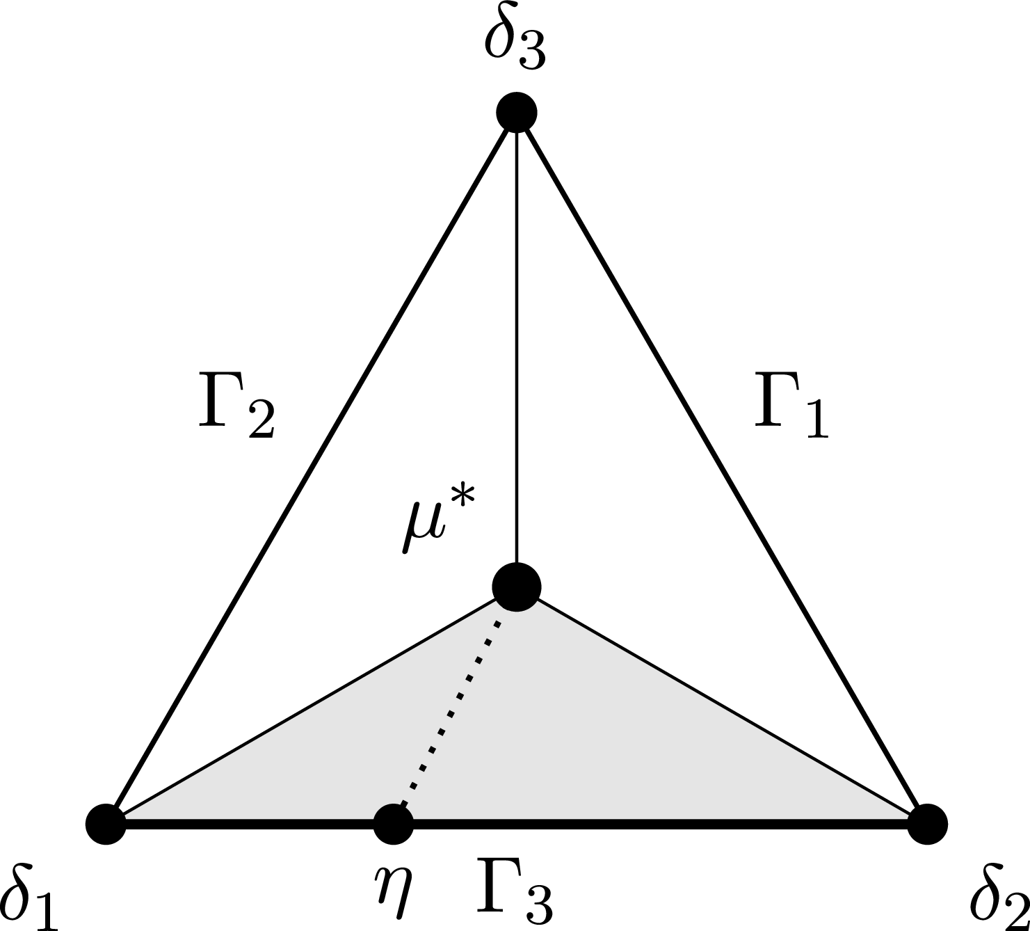
To do this, define the central measure $\mu ^{*}\in \Gamma$ by $\mu ^{*}(i)={1}/{(q-1)}$ for all $i \in [q] \setminus \{0\},$ and define the boundary face

\begin{equation*} \Gamma _i \;:\!= \; \{\mu \in R_i \;\vert \; \mu (i)=0\}\text{.} \end{equation*}

For example, Figure 1 depicts $\Gamma$ when $q = 4$ , so $\mu ^{*}(1)=\mu ^{*}(2)=\mu ^{*}(3)=1/3$ and $\mu ^{*}(0)=0$ .

For each $\eta \in \Gamma _i$ , we consider the two-dimensional cross section consisting of the measures

\begin{equation*} \Phi _i(\eta ,s,t) \;:\!= \; t\delta _0+(1-t)(s\mu ^{*}+(1-s)\eta)\text{,} \quad (s,t) \in [0,1]^2\text{.} \end{equation*}

For any $\eta \in \Gamma _i$ , we see that $\Phi _i(\eta ,0,0) = \eta$ , $\Phi _i(\eta ,1,0) = \mu ^{*}$ , and $\Phi _i(\eta ,0,1) = \Phi _i(\eta ,1,1) = \delta _0$ . Thus, these cross sections foliate the region $\left \{\mu _t \;\vert \; \mu \in R_i\;\text{and}\; t\in [0,1]\right \}$ , up to null sets.

Figure 1.

The region $\Gamma$ when $q = 4$ .

Proposition 3.7. Let $f \colon [q]^n \to \{0,1\}$ be a $0$ -monotone and symmetric function. There exists a constant $C(q)$ such that for any region $R_i$ , we have

\begin{equation*} \gamma \left (\{\mu _t\;\vert \;\mu \in R_i\;\text{and}\;t\in [0,1]\} \cap \mathscr{D}\right ) \leq C(q)\, \frac {\ln\!(1-\varepsilon )-\ln\!(\varepsilon )}{\log n}\text{,} \end{equation*}

Proof. Throughout the proof, $C = C(q)$ denotes different constants at different lines, depending on $q$ only. For $\eta \in \Gamma _i$ and $(s,t)\in [0,1]^2$ , we define

\begin{equation*} \Phi _i(\eta ,s,t) \;:\!= \; t\delta _0+(1-t)\bigl (s\mu ^{*}+(1-s)\eta \bigr )\text{.} \end{equation*}

For $s\gt 0$ , the measure $s\mu ^{*}+(1-s)\eta$ belongs to $R_i$ , and its $i$ th atom is

\begin{equation*} s\mu ^{*}(i)+(1-s)\eta (i)=\frac {s}{q-1}\text{.} \end{equation*}

Therefore, by Proposition3.6, for every fixed $\eta \in \Gamma _i$ and every $s\gt 0$ ,

\begin{equation*} \mathrm {len}\left (\left \{t\in [0,1]\;\vert \;\Phi _i(\eta ,s,t)\in \mathscr{D}\right \}\right ) \leq C\, \frac {(\!\ln\!(1/2) - \ln\!(\varepsilon ))\log\!((q-1)/s)}{\log n}\text{.} \end{equation*}

The slice $s=0$ is irrelevant for the following integration. We now integrate this estimate over all cross sections. The map $ \Phi _i\colon \Gamma _i\times [0,1]^2\to \Delta [q]$ parametrizes $\{\mu _t\;\vert \; \mu \in R_i\;\text{and}\;t\in [0,1]\}$ up to null sets. Moreover, in affine coordinates its Jacobian is of the form

\begin{equation*} c_q(1-t)^{q-2}(1-s)^{q-3}\text{,} \end{equation*}

and hence the density of the pullback of $\gamma$ under this parametrization is bounded above by a constant depending only on $q$ . Consequently, for every measurable set $B$ contained in the image of this parametrization,

\begin{equation*} \gamma (B) \leq C(q) \int _{\Gamma _i}\int _{0}^{1}\int _{0}^{1} \mathbb{I}[\Phi _i(\eta ,s,t)\in B]\,dt\,ds\,d\eta \text{,} \end{equation*}

where $d\eta$ denotes $(q-3)$ -dimensional Lebesgue measure on $\Gamma _i$ . Applying this with

\begin{equation*} B= \left \{\mu _t\;\vert \;\mu \in R_i\;\text{and}\;t\in [0,1]\right \}\cap \mathscr{D}\text{,} \end{equation*}

and then using the preceding line-segment bound, we get

\begin{align*} \gamma (B) &\leq C(q) \int _{\Gamma _i}\int _0^1 \mathrm {len}\left (\left \{t\in [0,1]\;\vert \;\Phi _i(\eta ,s,t)\in \mathscr{D}\right \}\right ) \,ds\,d\eta \\[3pt] &\leq C(q)\, \frac {\ln\!(1/2) - \ln\!(\varepsilon )}{\log n} \int _{\Gamma _i}\int _0^1 \log\!\left (\frac {q-1}{s}\right ) \,ds\,d\eta \text{.} \end{align*}

Finally, we note that

\begin{equation*} \int _0^1 \log\!\left (\frac {q-1}{s}\right )\,ds = \log\!(q-1)+\frac {1}{\ln 2} \leq C(q)\text{,} \end{equation*}

and the total $(q-3)$ -dimensional volume of $\Gamma _i$ is also bounded by a constant depending only on $q$ . Therefore

\begin{equation*} \gamma \left ( \left \{\mu _t\;\vert \;\mu \in R_i\;\text{and}\;t\in [0,1]\right \} \cap \mathscr{D} \right ) \leq C(q)\frac {\ln\!(1/2)-\ln\!(\varepsilon )}{\log n} \leq C(q)\frac {\ln\!(1-\varepsilon )-\ln\!(\varepsilon )}{\log n}\text{.} \end{equation*}

This proves the proposition.

3.6 Tightness

We remark that Theorem1.3 is sharp up to multiplicative constants. Ben-Or and Linial [Reference Ben-Or, Linial and Micali1] constructed the tribes function that showed that the $O(\!\log n/n)$ bound on influences presented by Kahn, Kalai, and Linial [Reference Kahn, Kalai and Linial4] is sharp. We present a generalized tribes function. Fix $q \geq 2$ , and let

\begin{equation*} \rho = \frac {2}{q+1}\text{.} \end{equation*}

Then $\rho \gt 1/q$ . Let $r$ be some positive integer, let $m = \left \lfloor \rho ^{-r}\right \rfloor$ , and set $n = mr$ . It is enough to construct examples for $n$ of this form. Partition the set $\{1,2,\ldots ,n\}$ into disjoint sets $T_1,T_2,\ldots ,T_m$ of equal size $r$ . For $a\in [q]$ and $x\in [q]^n$ , define

\begin{equation*} N_a(x)=\#\{i\in \{1,\ldots ,m\}\;\vert \;x_j=a\text{ for all }j\in T_i\}\text{.} \end{equation*}

We define $f \colon [q]^n \to [q]$ by

\begin{equation*} f(x)=\min \arg \max _{a\in [q]} N_a(x)\text{,} \end{equation*}

where the minimum is taken with respect to the order $0\lt 1\lt \cdots \lt q-1$ .

Note that the function $f$ is symmetric in the sense of Definition1.2. Indeed, $f$ is invariant under permutations of the blocks and under permutations of the coordinates inside each block, and this group acts transitively on $\{1,\ldots ,n\}$ . The function $f$ is also monotone. To see this, suppose $x\leq _a y$ . Then $ N_a(x)\leq N_a(y)$ and $ N_b(y)\leq N_b(x)$ for every $b\neq a$ . Thus, if $f(x)=a$ , then $a$ remains a maximizer after passing from $x$ to $y$ , and the tie-breaking order still selects $a$ . Hence $f(y)=a$ .

We now show that this construction gives the correct lower bound. Fix $0\lt \varepsilon \lt 1/2$ , and choose constants $c_-\lt c_+$ such that

\begin{equation*} -\ln\!(1-\varepsilon )\lt c_-\lt c_+\lt -\ln\!(\varepsilon )\text{.} \end{equation*}

For each $r$ , define $p_\pm \;:\!= \; p_\pm (r)$ by

\begin{equation*} p_-\;:\!= \;\left (\frac {c_-}{m}\right )^{1/r} \quad \text{and}\quad p_+\;:\!= \;\left (\frac {c_+}{m}\right )^{1/r}\text{.} \end{equation*}

Since $m=\lfloor \rho ^{-r}\rfloor$ , we have $p_+-p_-=\log\!((1-\varepsilon )/\varepsilon )\cdot \Theta (1/r)$ , provided that $c_+$ and $c_-$ are sufficiently close to $-\log\!(\varepsilon )$ and $-\log\!(1-\varepsilon )$ , respectively. Moreover, $r=\Theta (\!\log n)$ as $n=mr$ . Thus,

\begin{align*} p_+-p_-=\log\!((1-\varepsilon )/\varepsilon )\cdot \Theta (1/\log n)\text{.} \end{align*}

Choose $\delta \gt 0$ small enough so that

\begin{align*} \frac {1-\rho }{q-1}\lt \rho -2\delta \text{.} \end{align*}

This is possible because $\rho \gt 1/q$ . First consider $a\in [q]\setminus \{0\}$ . Let

\begin{align*} R_a= \{\mu \in \Delta [q]\;\vert \;p_-\leq \mu (a)\leq p_+ \text{ and }\mu (b)\leq \rho -\delta \text{ for all }b\neq a\}\text{.} \end{align*}

By the choice of $\delta$ , the sections of $R_a$ obtained by fixing $\mu (a)$ have volume bounded above and below by positive constants depending only on $q$ . Hence

\begin{align*} \gamma (R_a)=\Theta (p_+-p_-) =\log\!((1-\varepsilon )/\varepsilon ) \cdot \Theta (1/\log n)\text{.} \end{align*}

For $\mu \in R_a$ , set $ \lambda _a=m\mu (a)^r.$ Then $\lambda _a\in [c_-,c_+]$ . On the other hand, for $b\neq a$ ,

\begin{align*} \mathbb{P}_{x\sim \mu ^{\otimes n}}[N_b(x) \geq 1] \leq \mathbb{E}_{x\sim \mu ^{\otimes n}}[N_b(x)] = m\mu (b)^r \leq m(\rho -\delta )^r =o(1)\text{.} \end{align*}

By a union bound, no colour $b\neq a$ has an all- $b$ block with probability $1-o(1)$ , so

\begin{align*} \mathbb{P}_{x\sim \mu ^{\otimes n}}[\,f(x)=a] &= \mathbb{P}_{x\sim \mu ^{\otimes n}}[N_a(x)\geq 1]+o(1) \\[3pt] &= 1-(1-\mu (a)^r)^m+o(1) \\[3pt] &= 1-\exp\!(\!-\lambda _a)+o(1)\text{.} \end{align*}

By the choice of $c_-$ and $c_+$ , it follows that for all sufficiently large $r$ ,

\begin{equation*} \varepsilon \leq \mathbb{P}_{x\sim \mu ^{\otimes n}}[\,f(x)=a] \leq 1-\varepsilon \end{equation*}

for every $\mu \in R_a$ . Consequently,

\begin{align*} \gamma (\{\mu \in \Delta [q]\;\vert \;\varepsilon \leq \mathbb{P}_{x\sim \mu ^{\otimes n}}[\,f(x)=a]\leq 1-\varepsilon \}) \geq \log\!((1-\varepsilon )/\varepsilon ) \cdot \Theta (1/\log n) \end{align*}

for every $a\in [q]\setminus \{0\}$ .

It remains to prove the colour $a=0$ since the deterministic tie-breaking rule favours $0$ when no colour has a monochromatic block. In this case we use the colour $a=1$ as the competing colour. Define

\begin{align*} R_0= \{\mu \in \Delta [q]\;\vert \;p_-\leq \mu (1)\leq p_+\;\text{and}\;\mu (b)\leq \rho -\delta \;\text{for all}\;b\neq 1\}\text{.} \end{align*}

As before, $ \gamma (R_0)=\log\!((1-\varepsilon )/\varepsilon ) \cdot \Theta (1/\log n)$ . For $\mu \in R_0$ , set $ \lambda _1=m\mu (1)^r \in [c_-,c_+]$ , and note

\begin{align*} \mathbb{E}_{x\sim \mu ^{\otimes n}}[N_b(x)]=o(1) \end{align*}

for every $b\neq 1$ . Thus, with probability $1-o(1)$ , the only possible all-monochromatic blocks have colour $1$ . Hence

\begin{align*} \mathbb{P}_{x\sim \mu ^{\otimes n}}[\,f(x)=0] &= \mathbb{P}_{x\sim \mu ^{\otimes n}}[N_1(x)=0]+o(1) \\[3pt] &= (1-\mu (1)^r)^m+o(1) \\[3pt] &= \exp\!(\!-\lambda _1)+o(1)\text{.} \end{align*}

Again, by the choice of $c_-$ and $c_+$ , for all sufficiently large $r$ ,

\begin{equation*} \varepsilon \leq \mathbb{P}_{x\sim \mu ^{\otimes n}}[\,f(x)=0] \leq 1-\varepsilon \end{equation*}

for every $\mu \in R_0$ . Combining the two cases, for every $a\in [q]$ we obtain

\begin{equation*} \gamma (\{\mu \in \Delta [q]\;\vert \;\varepsilon \leq \mathbb{P}_{x\sim \mu ^{\otimes n}}[\,f(x)=a]\leq 1-\varepsilon \}) = \log\!((1-\varepsilon )/\varepsilon ) \cdot \Theta (1/\log n)\text{,} \end{equation*}

where the upper bound follows from Theorem1.3. This proves that the logarithmic dependence in Theorem1.3 is sharp.