2.1. The GLM Class

For a GLM, there is a monotone differentiable link function g(·) such that

mapping the mean response to a linear predictor defined in terms of regression coefficients β₁,…,β_p and γ₁,…,γ_q. Thus selecting which covariate components z_i,j to include amounts to determining which γ_j's to keep in the model; excluding component z_i,j corresponds to using γ_j = 0. For (classical) linear models, the link function is the identity function. For other examples, see Section 2.3.

We assume that Y₁,…,Y_n are independent with density function belonging to an exponential family of the form

where the sample space

is the same in each case and does not depend on the unknown parameters θ_i and φ. The functions a(·), b(·), and c(·,·) are fully specified. The b(·) function plays a crucial role because its derivatives yield the mean and variance function, whereas a(φ) is a scale parameter. From the two first Bartlett identities, about moment properties of the first and second log-derivatives of the density, comes the following expressions:

This expresses θ_i as a function of the mean response, given the covariates. When the so-called canonical link function is used, i.e., g(·) = (b′)⁻¹(·), then θ_i = g(ξ_i) = x_i^tβ + z_i^tγ.

2.2. The Pointwise FIC for GLM

Here we derive explicit expressions for the FIC when applied to the linear predictor μ = x^tβ + z^tγ = g(E(Y|x,z)) associated with a given position (x,z) in the covariate space. The (pointwise) FIC is large-sample equivariant under smooth transformations, and so the FIC for μ(x,z) will essentially yield the same model ranking as the FIC for ξ(x,z) = E(Y|x,z).

One of the main ingredients for computing the FIC is the (normalized) Fisher information matrix J_n,wide, computed via the second-order partial derivatives of the log-likelihood function with respect to (β,γ). We partition the matrix J_n,wide as

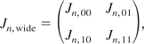
such that the block J_n,11 in the lower right corner has dimension q × q. In our calculations we frequently need the lower right submatrix of dimension q × q of J_n,wide⁻¹, which we name K_n. This matrix may be found as K_n = (J_n,11 − J_n,10J_n,00⁻¹J_n,01)⁻¹.

For several members of the generalized linear model family, the scale parameter φ is either known or completely specified. Examples are the Poisson and binomial distributions, where a(φ) = 1, or the normal distribution with known variance. In the case where φ is known, the information matrix takes a simple and general form, making it easy to compute in the full generality of GLMs. We first decompose the n × (p + q) design matrix into X = (x₁^t,…,x_n^t)^t of dimension n × p and Z = (z₁^t,…,z_n^t)^t of dimension n × q. Then

where V is the diagonal weight matrix diag(v₁,…,v_n), with different formulas available for v_i = v(x_i,z_i). One has

where η_i = g⁻¹(ξ_i) = x_i^tβ + z_i^tγ and ξ_i = E(Y_i|x_i,z_i) = b′(θ_i). For the situation with φ known, therefore, the K_n matrix takes the form

For canonical link functions, where θ_i = η_i, matters simplify to v_i = b′′(x_i^tβ + z_i^tγ).

When the scale parameter φ is not known, such as with the normal distribution with unknown mean and variance, or the gamma distribution, we shall argue that formula (3) is still valid for K_n. This is because of an orthogonality property, namely, that the mixed second derivatives of the log-likelihood function, with respect to φ and β or γ, are seen to have mean zero. Thus the full information matrix takes the form

where J_n,scale is the required

. This implies that the q × q lower right-hand corner of the inverse information matrix remains as in (3). For the normal distribution with φ = σ and a(σ) = σ², e.g., one finds J_n,scale = 2/σ².

We may now describe the FIC procedure for selecting the tentatively best model for estimating the focus parameter μ = μ(x,z) = x^tβ + z^tγ. The criterion works specifically for the given (x,z) position in covariate space; if required, the procedure can be repeated for several positions. Different submodels are indexed by the various subsets S of covariate components 1,…,q, ranging from the empty set to the full list. For each submodel S one can evaluate the estimate

that uses maximum likelihood estimates

in the model that employs all of β₁,…,β_p but only those γ_j for which j ∈ S. Here π_S is the |S| × q projection matrix that sends z to π_Sz = z_S, the vector of only those z_j for which j ∈ S, and |S| is the number of components in S. The essence of the FIC is to estimate the mean squared error for each candidate estimator and then to pick the one with lowest mean squared error estimate.

We need the vector ω = J_n,10J_n,00⁻¹(∂μ/∂β) − (∂μ/∂γ), which here reads

whether or not φ is known. Note the dependence of ω on (x,z). Note furthermore that premultiplying v_S = π_Sv with π_S^t produces a vector π_S^tπ_Sv of full length q, with zeros inserted for those components j with j ∉ S. Define next K_n,S = (π_SK_n⁻¹π_S^t)⁻¹, which is the |S| × |S| lower right block of the inverse of J_n,S, the information matrix for the S model, and let finally G_n,S = π_S^tK_n,Sπ_SK_n⁻¹. The value of the FIC is now obtained as

with

being the maximum likelihood estimator of γ in the largest of the considered models, i.e., the one containing all of γ₁,…,γ_q. For given values of (x,z), the best model according to the FIC is that model, indexed by S, for which FIC(S;x,z) is the smallest.

The FIC stems from estimating and then adding a squared bias term and a variance term; see Claeskens and Hjort (2003) for further discussion and applications. There is a modification of (5) for the case of the squared bias being estimated with a negative number; in such cases we truncate that term to zero. For further discussion of this point, see also relevant comments in Hjort and Claeskens (2006).

2.3. Examples

Here we present a short list of examples that fit in with the preceding general framework. Each model may be fitted using statistical software packages, and the J_n and K_n matrices are easily computed via the appropriate form of the v_i weights. For each situation one may use (5) to determine the best submodel for estimating x^tβ + z^tγ, or for any smooth function thereof, such as E(Y|x,z) or the median response median(Y|x,z).

3.1. Some Preliminary Results

Suppose in general terms that a parameter of interest μ(β,γ;u) depends on some quantity u that varies in the population being studied. Under the framework outlined previously, henceforth assumed to hold, the true parameter value is

. We shall now use results developed in Hjort and Claeskens (2003a) and Claeskens and Hjort (2003), with suitable modifications. These results rely on certain mild regularity conditions, detailed in these papers. One such condition that we need to mention here, to adequately identify the appropriate limits subsequently, is the existence of a limit matrix J to which J_n,wide converges, with blocks J₀₀, etc. Similarly this defines limit versions K of K_n and a fortiori J_S and K_S, limit versions of J_n,S and K_n,S. Also, K_S = (π_SK⁻¹π_S^t)⁻¹, the lower right block (J_S⁻¹)₁₁ of J_S.

For each u the theory as developed in Claeskens and Hjort (2003) applies to the subset-model-based maximum likelihood estimators

, for which we have the following convergence in distribution:

Here ω(u) = J₁₀J₀₀⁻¹∂μ(β,γ;u)/∂β − ∂μ(β,γ;u)/∂γ, with partial derivatives evaluated at the null point (β₀,0). Furthermore, M ∼ N_p(0,J₀₀) and D ∼ N_q(δ,K), and these random vectors are independent. The (M,D) variables are needed in Section 4, and furthermore the variables (C_S,D_S) that appear now are linear functions of (M,D).

For a fixed set S and a fixed focus point, Lemma 3.2 of Hjort and Claeskens (2003a) applies and yields

where

A special case of importance is that of S being the full set {1,…,q}, for which

For convenience of notation we adopt the notion that estimators without subset-subscript correspond to the full model, with all γ₁,…,γ_q parameters; thus

, etc.

The S-indexed model works with estimates

for γ_j with j ∈ S but uses 0 for j ∉ S. To deal efficiently with different functions of these it will be convenient to introduce the extended projection matrix of dimension (p + |S|) × (p + q),

With G_S = π_S^tK_Sπ_SK⁻¹, the limit version of G_n,S encountered in (5), we have

which is seen to have mean vector and variance matrix

3.2. The Case of No Common Parameters

In the previous section we assumed there to be a parameter vector θ common to all models. Often this is the case, e.g., in regression models when always including an intercept term. However, there are situations where one does not wish to include such a parameter in every model. Using the notation introduced earlier, this is the situation of only having a γ parameter (θ is not present). In fact, this simplifies the calculations quite a bit. Let γ₀ be the vector of null values for γ, where γ_j = γ_0,j corresponds to the jth modeling factor not being present. Most often γ₀ = 0_q, e.g., when modeling the mean in a GLM where γ_0,j = 0 indicates absence of covariate z_j, though other values are possible also. Consider, e.g., a skewed logistic regression model where the probability of success is

Here γ = (β,η) and γ₀ = (0,1). The computation of the Fisher information matrix is simpler because we now do not have to take derivatives with respect to θ. One finds that the full Fisher information matrix

for the situation without common parameter θ is equal to the lower right block J_n,11 of the partitioned matrix in the (θ,γ) situation. Equivalently,

. To avoid confusion, we place a tilde above matrices to denote the situation of the case of no common parameters. Define the score function

. By a Taylor expansion around

, under the local misspecification setting, it follows that

, where

. This implies that

. From this it follows that

Defining

and

, we have

, where

corresponds to

, the limiting distribution of

. It now immediately follows that

Hence, with

,

. This limiting variable Λ_S has mean

and variance

. Except for the simplified forms of the matrix

and the vector

, this distribution differs from that in the (θ,γ) situation by the absence of a variance term for the model only containing θ. The risk function or mean squared error corresponds to

. We now proceed by inserting the unbiased estimator

for δδ^t and replacing unknown parameters by their maximum likelihood estimators in the full model. Substituting

,

, and

for ω, G_S, and J, the formula (5) for the pointwise FIC remains valid for the case of no common parameters.

3.3. The wFIC for GLM

Consider again the linear predictor μ(x,z) = x^tβ + z^tγ and the collection of submodel-based estimators (4). The vector

is always of length p but takes on different values for different index sets S. In contrast, the estimator

has length |S|. The construction of the wFIC proceeds as follows. As opposed to using the pointwise loss function, we start with the weighted average quadratic loss function on the scale of the linear predictor, of the form

The weights w(x_i,z_i) are user-specified and in general different from the weights v(x_i,z_i) in the GLM weight matrix V. We shall show that this random loss has a limit distribution, under mild regularity conditions. Let

and assume this matrix converges in probability to a nonnegative definite Ω_w, depending of course on the weight function w(x,z).

To properly study the random loss function it is convenient to express it as

From conditions and results noted earlier,

Under mild conditions, the expected loss w-risk_n(S) = E L_n(S) will converge to w-risk(S,δ) = E L(S). The limit loss L(S) is a quadratic form in normal variables and has mean value

involving matrices F_S and Γ_S defined previously. We see that the I(S) term corresponds to weighted squared bias, whereas the second term II(S) is related to weighted variance. By earlier efforts, this second term can be expressed as

.

This leads upon estimating unknown quantities to a wFIC. The second term is not problematic, and we use

where

is the appropriate submatrix of

and

is the estimated version of (2), inserting

for the linear predictor x_i^tβ + z_i^tγ. See the examples in Section 2.3. For the first term, we note that

a variable with mean δδ^t + K; recall the convention noted around (6) that

means

, etc. Hence

is an asymptotically unbiased estimator of I(S), and

an asymptotically unbiased estimator of w-risk(S,δ). To avoid estimating a nonnegative quantity with a negative number, we advocate truncation to zero, and we use

. The wFIC consists in evaluating

for each candidate model S and in the end selecting the model with smallest value of this estimated average risk. All components of the preceding expressions are easily obtained via standard output of any software fitting GLMs.

Remark 1. When more components are put into S, the I(S) term becomes smaller; for S equal to the full {1,…,q} we find F_S = 0, making I(wide) = 0. On the other hand, the more components in S, the bigger is the variance II(S). Thus the wFIC method reflects the squared modeling bias against variance balance.

Remark 2. The

is not algebraically equivalent to the simpler one of averaging individual FIC(S) scores. The two methods are the same only in cases where there are no modifications of setting negative estimates of squared bias to zero. The wFIC method, as outlined in Sections 3 and 4, performs the squared bias modification only once, at the end, as opposed to performing this operation for each individual application.

Remark 3. The methods stem from precise limit distribution results that involve quantities such as J and K, along with further relatives such as K_S and G_S. Our wFIC(S) formulas involve estimates of these quantities,

,

, etc. The theory behind the methods ensures that they work well as long as estimates are used that are consistent, under the local misspecification framework

. Among various possibilities we have chosen to use the “wide model perspective” in our implementations, starting from estimators

that use estimates

.

3.4. Examples Revisited

Here we make the formula for wFIC much more explicit for the class of GLM examples, with particular attention to the classical linear model. Again we use V = diag{v_i} and W = diag{w(x_i,z_i)}. Examples of v_i for the case of the linear, Poisson, binomial, and gamma models are given in Section 2.3. We turn to the choice of weights w(x_i,z_i) in Section 6.

First we work with

of (9). With J_n,wide as in (1), G_S = π_S^tK_Sπ_SK_n⁻¹, and K_n as in (3), one has

Next we simplify the matrix multiplications needed to compute

. After rearranging the resulting terms and introducing the generalized “hat matrix” for GLM,

, we arrive at

, and hence

. For

we need the matrix J_n,S, which is that submatrix of J_n,wide for which the row and column indices belong to the index set S. For example, if S = {3,5} this gives the parameter μ_S(x,z) = x^tβ + z₃γ₃ + z₅γ₅. In this example, of the matrix J_n,S we keep of the last q rows only rows 3 and 5, and of the last q columns we keep only columns 3 and 5. In general, for any subset S of {1,…,q}, we denote the reduced design matrix Z_S = Zπ_S^t and

Using formulas for the inverse of a partitioned matrix,

, and

This leads to

and finally to wFIC(S) as in (9). These expressions are straightforward to program.

In the special case of the classical linear model, the “hat matrix” is H = X(X^tX)⁻¹X^t, and

with B_S¹¹ = {Z_S^t(I_n − H)Z_S}⁻¹ and again with wFIC(S) being the sum of these two terms.

Remark 4. In linear models the expression for the pointwise (unweighted) FIC has been shown to be exact; see Claeskens and Hjort (2003, Sect. 5.5). There it is shown that, without assuming normality and when using least squares estimators, the exact expression for the mean squared error matches that obtained by FIC. This is a favorable property that helps in appreciating the obtained expression for the FIC. More precisely, in a linear model with Y_i = x_i^tβ + z_i^tγ + ε_i, where μ = x^tβ + z^tγ is to be estimated, we use least squares estimators in a submodel indexed by S, leading to the estimator

. Computing the exact bias and variance of this estimator leads to the following expression for the mean squared error of

:

This is, up to a constant not depending on the subset S, identical to the limiting expression on which the FIC is based; compare with (5). The same property holds when a (nonrandom) weight function w is included in the loss function L_n in (7). For linear models, computing the exact mean squared error of L_n(S), with least squares estimators inserted for

and

, leads to an expression that is equivalent to that upon which wFIC as in (9) is based. Note that the error variance σ² appears in the denominator of the matrix J_n as the scaling factor a(σ). There is accordingly a σ² factor implicitly featuring in the first two terms of (10) but not in the final term.

6.1. GLM Weights

The log-likelihood structure of a GLM itself suggests a type of weights for use in the wFIC method. If one chooses w(x_i,z_i) = v_i/a(φ), then Ω_n,w = J_n,wide. This leads to simplifications in the w-risk(S,δ) and wFIC(S) expressions, as we shall see now. For simplicity of notation and presentation we work directly in the limit experiment, where J and K, etc., replace

and

, etc.; we also write G_S = π_S^tK_Sπ_SK⁻¹. First look at I(S) = δ^tF_S^tJF_Sδ, where some manipulations give

This leads with some further efforts to

which is estimated by

as long as this expression is positive; it is otherwise truncated to zero. Next,

This is easily obtained because the effect of pre- and postmultiplication by

is that only that submatrix of J⁻¹ is kept for which the row (and column) numbers belong to the index set S, entries on all other rows and columns being replaced by zero. This implies that J is multiplied by part of its inverse matrix, leading to the simplification p + |S|. This is also true for the data-based version

.

To summarize this, with GLM weights the limit risk takes the form

and the canonical risk estimate (for the limit experiment) is

Here N(S) is the event that the trace in

is positive, i.e., D^t(K⁻¹ − K⁻¹π_S^tK_Sπ_SK⁻¹)D > q − |S|. The N(S) takes place with high probability if δ is some distance away from zero, but in situations where the underlying γ vector is close to zero, i.e., the narrow model is close to being correct, the probability that N(S) does not take place is significant. The finite-sample version of the risk estimate uses

for D and

and

for K and K_S.

6.2. The wFIC and the AIC

Consider the AIC, which in the present circumstances takes the form

with

being the appropriate maximum likelihood estimate of θ_i = θ(x_i,z_i), which again depends on

and

. The AIC scores may be computed for each submodel S, down to that of the most narrow model, which corresponds to S = [empty ] and which uses only β₁,…,β_p,φ as model parameters. When subtracting the smallest model's AIC value from AIC(S), and performing a one-step Taylor expansion, we find that, for the limiting situation where n → ∞,

See Claeskens and Hjort (2003, eqn. (2.5)). The best models have the highest AIC scores.

We see from this and (14) that the wFIC method, when using GLM weights, is essentially large-sample equivalent to the AIC method. The word essentially relates to the modification for truncating an estimate of a squared bias to zero, when relevant, spelled out in (14). Thus the wFIC provides a fresh perspective on the AIC, and our arguments even suggest a correction to the AIC scores in cases where the event N(S) does not take place. The result just described generalizes further, to the setting of Section 4. When the A matrix of (13) is proportional to K⁻¹, then the wFIC and the AIC are large-sample equivalent, inside the framework of local neighborhood models.

It is interesting to go through the list of examples in Section 2.3 to see the appropriate random loss functions that correspond to the AIC. For the logistic regression setup of Example 3 in that section, e.g., model selection by estimating the mean of

is essentially the same as AIC. Here

is the estimated probability under model S. Similarly, for Poisson regression, basing model selection on estimating

will be large-sample equivalent to the AIC scheme, where

is the estimate of Poisson rate i inside the S model. Of course other weights and other transformations can be worked with, for logistic and Poisson regression, and such alternatives can in the perspective developed here be seen as cousins to the AIC method.

6.3. Other Types of Weights

In addition to the perhaps canonical GLM weights choice discussed previously, the following types of weights may be considered. We emphasize again that choosing an appropriate weight function is a context- and application-dependent issue.

Uniform weights. A simple choice of weights could just assign mass 1/n to each contribution in the summand, with the Ω_n matrix simply equal to the empirical variance matrix of the p + q-sized covariate vectors. Another choice is to let w_i = 1 precisely for individuals i belonging to a stratum of interest and w_i = 0 for the others. This is exemplified in Section 7.

Gliding covariate window. A version of the preceding situation is to use w_i = w(x_i,z_i;x₀) equal to 1 for individuals inside a certain neighborhood of some fixed x₀. This gives a ranking of candidate models around each fixed x₀. Smoothed versions can also be contemplated, also in a context of model assessment where the x₀ is moved in its covariate space. A good final model, then, should rank highly in all these local competitions.

Averaging over z for fixed x. Another version with some appeal is to assess models in terms of how well they perform for a given covariate x, averaged across all likely z values. To indicate in one particular fashion how this may be handled, let

in terms of the density f of the multinormal density N_q(0,Σ_x), where ξ_x and Σ_x are the estimated mean and variance matrix for z given x.

Dimension reduction for discriminant analysis. Assume that a classifier is to be constructed for discriminating between two populations 0 and 1 with prior frequencies π₀ and π₁. For given models for the two populations, say, f₀(x,θ,γ) and f₁(x,θ,γ) in terms of the feature vector x, where θ signifies protected and γ open parameters, the optimal classifier says “1” if π₁f₁(x) > π₀f₀(x) and “0” otherwise. Using ordinary direct likelihood methods to estimate parameters and deciding on a good submodel, e.g., via the AIC, is often not adequate, because effort is spent to estimate densities well where it does not really matter. What counts for good classification is to estimate log-densities well where log f₁(x) − log f₀(x) is close to the threshold c = log(π₀/π₁). The wFIC may be used for such purposes, taking as a departure point loss functions of the type

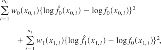
with weight functions w₀ and w₁ chosen in a suitable fashion such that weights are large in the (estimated) area where the log-density difference is close to the threshold c. Here x_0,i and x_1,i denote training vectors from populations 0 and 1.

Robust weights. There is a whole area of research addressing issues related to robust model choice. Robustness is concerned with the downweighting (and sometimes identification) of data vectors that are “outliers” or that may exert too strong an influence on maximum likelihood estimators. The methodology developed in this paper sticks to the maximum likelihood estimators, as such, but the weight function of the wFIC allows downweighting schemes that make model selection less dependent on extreme data vectors. One version of this would be

where the norm in question could measure a suitable distance from covariate vectors to some robustly identified center location (x₀,z₀) and where h(u) could be taken as 1 over a broad interval but made to go to zero beyond that interval. Another choice is h(u) = exp(−c|u|) for a perhaps small value of c. Such a scheme assures robustness with respect to extreme or overly influential covariate vectors.

Note before we come to the next point that the wFIC methodology also works with weights more general than w_i = w(x_i,z_i), as long as the Ω_n,w matrix of (8) converges in probability. Thus weights of the form w_i = h(res_i), functions of suitably defined GLM residuals, are allowed. One such version, among several, is

where

, featuring (perhaps robustified) estimates of mean and standard deviation for Y_i. Weights of this type are discussed, in a rather different context of robust linear regression, by Ronchetti and Staudte (1994), who also find that c = 1.345 is a reasonable default value for this weight function.

Weights in general regression models. In the more general framework of Section 4, selecting weights appropriate for the occasion amounts to specifying first the relevant class of focus estimands μ(u) and then a weight function W for the u index. This is tantamount to constructing the weight matrix A of (13); see the illustration in Section 7.1.

7.1. Quantiles for Wage Distributions

For the following illustration of our methodology we shall consider the data set cps85.data, available from the Internet, pertaining to a random sample of 528 individuals from the 1985 Current Population survey by the U.S. Census Bureau; for a brief discussion, see Hansen (2007, p. 31). Eight covariates are recorded for each individual, along with the person's hourly wage (in dollars). We order these covariates as x₁, length of education, in years; x₂, gender (1 if female, 0 if male); x₃, potential labor market experience, in years; x₄, union status (1 if in union job, 0 if not); z₁, region of residence (1 if south, 0 if not); z₂, indicator for nonwhite and non-Hispanic; z₃, indicator for Hispanic; and z₄, indicator for being married. The statistical task is to model and then analyze, how these influence the salary level. Our notation reflects the modeling decision to keep the four x_j's protected (viewing it as prior knowledge that these variables have a bearing on salary) whereas the z_j's may or may not enter the finally selected model. Because salary distributions tend to be log-normal, and the data exhibit variance heterogeneity, our widest model takes log-salary Y_i for individual i to be normally distributed with mean ξ_i a linear function in the eight covariates and with standard deviation σ_i, also allowed to depend on covariates.

Write ξ_i = x_i^tβ + z_i^tγ, where in our application x_i = (1,x_i,1,…,x_i,4)^t and z_i = (1,z_i,1,…,z_i,4)^t, and σ_i = σ exp(v_i^tκ), where v_i depends on the covariates. Here we normalize the v_i's so as to have mean zero, for simplicity of both computation and interpretation; thus σ is the standard deviation for Y_i's for which v_i is equal to the average value zero. We shall in fact take σ_i = σ exp(κ₁x_i,1′ + κ₃x_i,3′), with x_i,1′ = (x_i,1 − x₁)/sd(x₁) and x_i,3′ = (x_i,3 − x₃)/sd(x₃). The narrow model has p = 1 + 5 parameters (σ and four β_j's) whereas the wide model has an additional q = 4 + 2 parameters (four γ_j's and two κ_j's). A total of 2⁶ = 64 candidate models is considered, corresponding to setting subsets of the six extra parameters to zero.

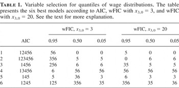
After a careful scrutiny of the data we removed four outlying individuals (salary of nos. 247, 270, and 348 is too high and salary of no. 502 is too low) to avoid parameter estimates and hence model selection mechanisms being overly influenced by highly unusual data values (outside the 0.999 probability range under the assumed regression structure). We first computed AIC values for all models, and the five best are 12456, 123456, 1456, 13456, and 145. In this notation, “145,” e.g., means including γ₁,γ₄,κ₁ in the model while setting γ₂,γ₃,κ₃ to zero, and “0” and “123456” correspond to the two extreme models of the narrow and the wide. That variance heteroskedasticity is called for is clear from the fact that the best variance homogeneous model (124 actually) is only ranked no. 25 on the AIC preference list.

To compute FIC and wFIC values we start with the log-densities of the model,

Computing derivatives with respect to σ,β,γ,κ at the null model where γ = 0 and κ = 0 yields (ε_i² − 1)/σ,ε_ix_i/σ,ε_iz_i/σ,(ε_i² − 1)v_i, in terms of ε_i = (Y_i − ξ_i)/σ_i. Because these are independently and identically distributed (i.i.d.) standard normal, one finds the normalized information matrix

where

These are of sizes 9 × 9 and 2 × 2 in the application. For a given focus estimand μ = μ(σ,β,γ,κ), the general method of Section 4 leads to

Also, K_n = diag(σ²Σ_n¹¹,½L_n⁻¹), with Σ_n¹¹ the lower right 4 × 4 block of the inverse of Σ_n. From this we may compute all 64

matrices, involving the maximum likelihood estimate

computed from the widest model, and all 64

matrices. Actually, the scale factors cancel each other for G_n,S, and so these matrices are observed without estimation noise.

The apparatus of Section 4 may now be applied for each given class of relevant estimands, such as probabilities of low wages as a function of covariates within certain strata of workers, the ratio of men's wages to women's wages, etc. Here we choose to consider quantiles of the wages per hour distribution for given covariates, i.e.,

where v is determined by x, as detailed previously, and c is the appropriate normal quantile. We shall focus on married women in unionized work, living in the south region, with both race indicators z₂ = z₃ = 0, and we consider the salary quantile as a function of the length x₁ of the woman's education. In other words, our focus is the function μ(x₁) = μ(x₁,σ,β,γ,κ) emerging from the preceding formula for covariate vectors (1,x₁,1,x_3,0,1,1,0,0,1)^t, when x₁ traverses the sampled values (from 6 to 18 years), for some fixed length of work experience x_3,0. There are 2⁶ different curve estimates

, one for each submodel.

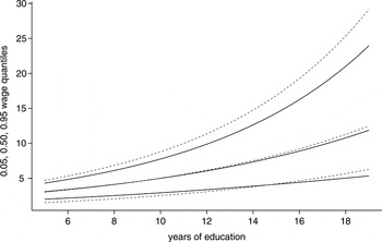
Table 1 gives the best six AIC models, along with the best six wFIC models, for the 0.95, 0.50, 0.05 quantile functions and for x_3,0 set equal to, respectively, 3 years and 20 years, for the stratum of married women described previously. Figure 1 gives quantile curves for the case of x_3,0 being 3 years, with estimates stemming both from the AIC-best model and for those found by the wFIC mechanism. Similar analyses for other functions of other covariates and for other strata of workers can easily be carried out, in each case leading to different lists of top models. That such versatility and flexibility of method are of importance and relevance in econometric model selection situations is also discussed in Hansen (2005). Note that all n = 524 data vectors are used to estimate the wage quantiles for each stratum.

Variable selection for quantiles of wage distributions. The table presents the six best models according to AIC, wFIC with x3,0 = 3, and wFIC with x3,0 = 20. See the text for more explanation.

Quantiles for wages: estimates of the 0.95, 0.50, 0.05 quantile curves for hourly wages for the stratum of women described in the text, as a function of the length of their education, when the work market experience x3,0 is fixed equal to 3 years. The AIC-model-based estimates are given with full lines, whereas the dotted lines refer to estimates based on the best wFIC model, with better estimated precision.

7.2. Diabetic Retinopathy Data

The Wisconsin Epidemiologic Study of Diabetic Retinopathy (see Klein, Klein, Moss, Davis, and DeMets, 1984) provides information for studying how diabetic retinopathy may be influenced by several other measurements. The data set consists of patient information for 348 men and 343 women. The binary outcome variable Y = 0 indicates that there is no or only mild nonproliferate retinopathy for both eyes. A value Y = 1 corresponds to moderate to severe nonproliferate retinopathy, or proliferate retinopathy, for one or both eyes. Previous analysis of similar data, in addition to prior knowledge among ophthalmologists, suggests that duration of diabetes in years (x₁) and presence of macular edema in at least one eye (x₂) are of direct relevance for the outcome of Y, and so these are protected covariates in each of the models that we shall consider. Further covariates, seen as candidates for inclusion in a final model, are percentage of glycosylated hemoglobin (z₁), body mass index (z₂), pulse rate in beats per 30 seconds (z₃), sex (z₄, with 1 for male and 0 for female), presence of urine protein (z₅), and area of residence (z₆, 1 or 0 for urban or rural).

A logistic regression model is used for the analysis. This means that the

matrix is diagonal with elements

, where

with H(u) = exp(u)/{1 + exp(u)} the logistic transform. Here β₀ is the intercept, whereas x_i = (x_i,1,x_i,2)^t and z_i = (z_i,1,…,z_i,6)^t are the covariate parts for individual i, for i = 1,…,n = 691. At the full model, we obtain estimates −6.344, 0.084, 2.036, 0.069, 0.031, 0.039, 0.119, 1.035, 0.241 of the nine parameters, with corresponding standard errors 1.148, 0.011, 0.411, 0.054, 0.026, 0.017, 0.231, 0.276, 0.228. Here the intercept and variables x₁,x₂,z₅ are highly significant, and variable z₃ is associated with a p-value of 0.022. The other variables are individually not significant.

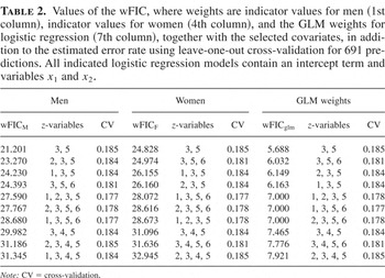
We perform model selection among all six z variables and allow for all possible subsets of the full model, leading to 64 candidate models. As model selection criteria we take first wFIC_M(S) with indicator weights w_i = I(i is male) and next wFIC_F(S) with weights w_i = I(i is female). Note that the values of wFIC(S) are computed using the complete data set; we are not splitting the data set for model selection. We furthermore consider wFIC_glm with the GLM weights for logistic regression, which translates to taking

. Table 2 gives for the three wFIC criteria the top 10 models, identified by their z covariates, along with their associated wFIC scores. The versatility of our method could be further illustrated by choosing other weight functions; thus

would give extra emphasis to models that do well for patients with high Y = 1 probabilities, whereas

corresponds to finding models that do better for those with low Y = 1 probabilities.

Values of the wFIC, where weights are indicator values for men (1st column), indicator values for women (4th column), and the GLM weights for logistic regression (7th column), together with the selected covariates, in addition to the estimated error rate using leave-one-out cross-validation for 691 predictions. All indicated logistic regression models contain an intercept term and variables x1 and x2.

For this particular illustration, the best wFIC model turns out to be the one with variables z₃ and z₅, for each of the three setups. This happens to correspond precisely to those variables that were found individually significant in the full model at the 5% level. For other weight schemes, different submodels are selected. The three wFIC schemes differ in the ranking of the following top candidate models. From Table 2, there is some indication that the body mass index (variable z₂) is more important for men, whereas the area of residence (z₆) may be more important for women. Thus we learn that, e.g., body mass index influences Y in possibly different ways for men and for women, which may be taken into account for building a final model or for carrying out the most appropriate model averaging for prediction; see the discussion in Section 9. We note further that the model ranking based on wFIC_glm is very similar to that based on the AIC.

It is important to note that the wFIC method aims at obtaining a good approximation to the full probability surface function p(x,z) = P(Y = 1|x,z), across values of (x,z), with appropriate and user-defined weights w(x,z). This is different from the aim of finding a model that produces the lowest possible error rate when used for discriminant analysis purposes. Such an aim relates to the more crude task of sorting individuals into “Y is probably 1” and “Y is probably 0” classes, based on (x,z). Thus it is not surprising that some submodels have slightly better error rate properties than those found best from the wFIC perspective. Examining estimated error rates for the 64 different logistic regression–based classifiers (via leave-one-out cross-validation), the primary feature is that they are all rather similar, spanning a tight range from 0.175 (121 errors of 691) to 0.190 (131 errors of 691). The tentatively best models, from this classification accuracy point of view, are 1256 (error rate 0.175), then 1356, 13456, 125, 12456, 12356 (each with error rate 0.177); here “1256” identifies the model with variables z₁,z₂,z₅,z₆, etc. Entirely similar results are found using, e.g., ten- or fivefold cross-validation. For some further discussion of predictive properties of different models we refer to Claeskens, Croux, and Van Kerckhoven (2006).

7.3. Highway Data

To illustrate robust downweighting, we use Hoffstedt's highway data; see also Weisberg (2005, Sect. 7.2). This data set is used to explain the 1973 accident rate per million vehicle miles as a function of several variables. There are 39 observations made. In every model we include an intercept term and x₁, the length of the highway segment in miles. Additional variables to choose from, when searching for an overall good model, are average daily traffic count in thousands (z₁), truck volume as a percentage of the total volume (z₂), total number of lanes of traffic (z₃), number of access points per mile (z₄), number of signalized interchanges per mile (z₅), number of freeway-type interchanges per mile (z₆), speed limit in 1973 (z₇), lane width, in feet (z₈), width of the outer shoulder on the roadway (in feet) (z₉), and finally an indicator of the type of roadway or the source of funding for the road (z₁₀).

Based on robust C_p model selection, Ronchetti and Staudte (1994) support the model that includes, in addition to x₁, the variables z₅, z₆, z₇, and z₁₀, and also the model with additional variables z₂, z₃, z₄, and z₉. Here we construct weights w₁,…,w₃₉ based on the robustification method outlined in Section 6.3; these rely on initially used robust estimators for the regression coefficients obtained in the full model. Five of the observations receive a weight that is smaller than one; all other observations get weight one. The weights that differ from one are 0.903, 0.568, 0.436, 0.577, 0.811. These weights are then used in the wFIC(S) construction and lead to preferring the model with the two variables x₁ and z₁₀. For this particular example, the model selected by wFIC is more parsimonious than the model suggested by the robust C_p.

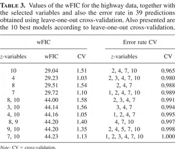
Table 3 presents, in a manner similar to Table 2, the 10 best wFIC values, the corresponding models, and the corresponding leave-one-out prediction error

computed in that model. Each time, the values (y_i,x_i) are left out when computing

, where we write x_i = (1,x_i,1,z_i,1,…,z_i,10)^t. The 10 best models according to the leave-one-out prediction error are also presented. The wFIC with robustified weights has larger estimated prediction error than the best models obtained with leave-one-out cross-validation. The model selected by the wFIC method tends for this example to be more parsimonious than the model selected by cross-validation. One should keep in mind that minimizing prediction error was not the goal for the computed values of the FIC.

Values of the wFIC for the highway data, together with the selected variables and also the error rate in 39 predictions obtained using leave-one-out cross-validation. Also presented are the 10 best models according to leave-one-out cross-validation.

8.1. The Real Risk Function

Consider estimators of the type

, where

is the submodel selected by, say, AIC or the wFIC. A more general class is that of

where the model weights are allowed to depend upon data and where the sum is over all candidate models (e.g., all inside a nested sequence). The AIC method corresponds to c_n(S) = 1 for precisely the set S selected by the AIC, with c_n(S) = 0 for the other models, etc. Suppose that the collection of model weights c_n(S) is such that they converge jointly to c(S|D), in the limit experiment associated with variables (M,D) in (11). For this broad class of estimators-after-selection, and more generally model average estimators,

where δ*(D) = [sum ]_Sc(S|D)G_SD. This follows essentially via simultaneous convergence of all variables involved in (11) and the random weights, in combination with the continuity theorem of weak convergence. The important consequence is that we may describe what happens to the real random loss L_n* = n ∫{μ*(u) − μ_true(u)}²dW_n(u) incurred by the statistician's strategy, as opposed to only the random loss for strategies using predetermined models. For the real loss we have

From this we also infer the large-sample limit of the real risk function (again after subtracting the irrelevant ∫τ₀²dW term),

in which bias(δ) and var(δ) are used to denote the q-dimensional bias function and q × q variance matrix of δ*(D). The specifics of the model selection or average strategy (16) determine these bias and variance functions; recall that D ∼ N_q(δ,K). Also, A = ∫ωω^tdW, as before. We may note that (13) is a special case of the general result (18).

Result (18) covers both the AIC and wFIC strategies, along with smoothed versions thereof (and the original FIC scheme corresponds to the weight measure being concentrated in a single point). That the AIC method is inside the required class essentially follows from (15), which implies that there is joint convergence, with c_n,aic(S) →_d c_aic(S|D), the latter defined as the indicator for the set S for which aic(S) = D^tK⁻¹π_S^tK_Sπ_SK⁻¹D − 2|S| is larger than all other aic(S′). Similarly, the wFIC method uses random weights c_n,fic(S) that converge jointly to c_fic(S|D), defined as the indicator for the set S for which

is smaller than all other I

*(S′) + II

*(S′). This follows because

whereas the other quantities are estimated consistently in our local

neighborhood formulation.

8.2. Comparing AIC with wFIC

The performances of different model selection or model averaging strategies may be compared using (18). Space does not allow us any deep investigation into the pros and cons of different methods, but we shall attempt to explain here that there will be many situations where the wFIC method will perform better than the AIC, for large regions of the parameter space.

Let us assume, for simplicity of presentation, that the K matrix is diagonal, with diagonal elements, say, κ₁²,…,κ_q², and that the list of candidate models corresponds to all 2^q subsets of {1,…,q}. The right-hand side of (15) then becomes aic(S) = [sum ]_j∈S(D_j²/κ_j² − 2), and one finds that (the limit experiment version of) AIC selects the set of j for which

. The AIC therefore acts as a pretest screener for each nonprotected parameter, actually using significance level 0.157 per parameter; the performance of other pretest methods, with harder or softer screening thresholds, can also be analyzed via (17). We can therefore compute the bias_aic(δ) and var_aic(δ) for the AIC method, via

for j = 1,…,q. These considerations determine the AIC performance as

Note that AIC selects these j regardless of the context-driven loss function, i.e., regardless of the matrix A = ∫ωω^tdW.

The wFIC, on the other hand, selects components with specific regard to A, i.e., to what is deemed important when setting up the loss function in the first place. One may show here, under the diagonal K assumption, that wFIC selects S to give smallest value of h(S) = [sum ]j∈S2aj,jκj2 + DSctAScDSc, with Sc the complement of S. Note, e.g., that if the loss function gives an A matrix with some components j that do not matter, then wFIC does not include them, whereas AIC is programmed to take these on board also, even when this gives an extra yoke of sampling variability. Similarly, if some aj,j components are much larger than others, potentially contributing harshly to the risk in (18), then wFIC tends to avoid including the associated γj's in the model.

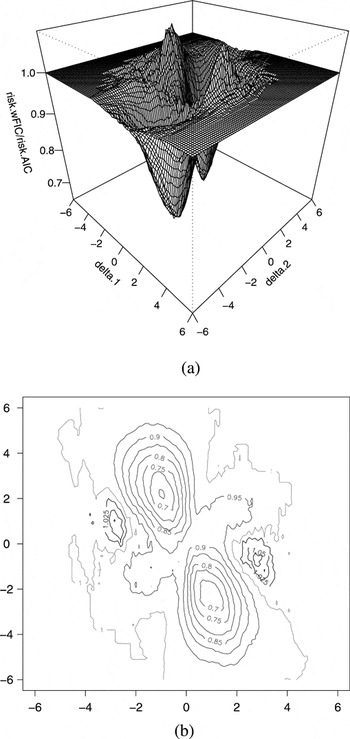
We compared the AIC to the wFIC in the limit experiment situation. We took q = 2, which allows us to present the results graphically, and we let δ₁, δ₂ take values in an equispaced grid of 200 points between −6 and 6. For each such combination of “true” values of δ = (δ₁,δ₂), 2,000 values for D were simulated from a bivariate standard normal distribution. We proceeded by performing wFIC and AIC model selection for each simulated value of the vector D to obtain the value of the indicator weight c(S|D), which is either 0 (if the model is not selected) or 1 (when that model is selected) for the four candidate models, which we label “0” (none of γ₁,γ₂ included), “1” (γ₁ included, γ₂ not), “2” (γ₁ excluded, γ₂ included), “12” (both included). This allowed us to compute values of bias(δ) = E(δ*(D) − δ) and of var(δ) = var(δ*(D)) for wFIC and AIC model selection. The A matrix taken was

Figure 2 depicts the ratio of the risk values for wFIC by those of AIC. Values below 1 indicate preference for the wFIC, whereas values above 1 are situations where AIC has lower risk. There is no absolute preference of one method above the other. The risk ratio surface converges to 1 when ∥δ∥ increases. The figure indicates a significant area in δ-space where wFIC has better performance. In these areas wFIC has a much lower minimal risk than that of AIC. The risk function, computed via equation (18), takes values between 5.216 and 229.914 for wFIC. For AIC the minimal simulated risk is larger, with value 5.704, whereas the upper bound is the same. Computations for the risk ratio of wFIC/AIC lead to a lower bound of 0.643; i.e., the risk for wFIC is only 0.643 times that of the AIC for certain values in δ-space, whereas the maximum of this ratio is equal to 1.090, indicating only a slight advantage for the AIC in those areas where it has a better risk.

(a) Simulated risk ratio wFIC/AIC for model selection in a situation with q = 2, K the identity matrix, and the matrix A as given in the text. Values below 1 indicate preference for wFIC; values above 1 indicate preference for AIC. (b) Contour plots of the risk ratio wFIC/AIC.

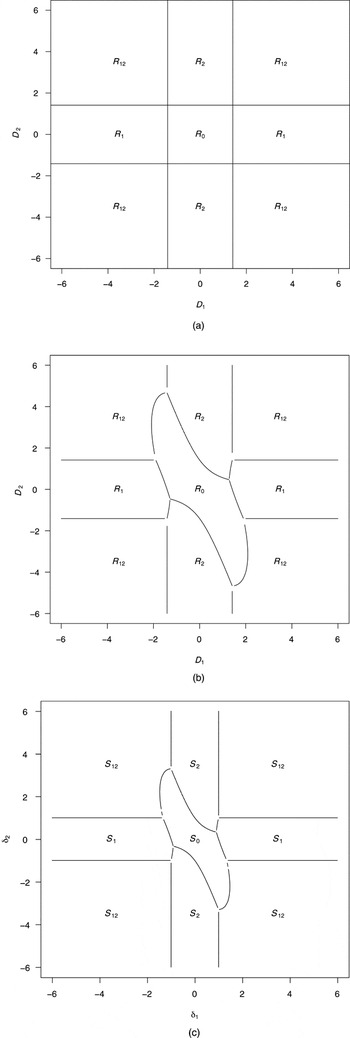
Because the limit version of AIC selects those variables with index j for which

, the areas where AIC selects a certain model are easy to depict; see Figure 3a. For the same grid of D₁, D₂ values we can use wFIC model selection and obtain information on the D₁, D₂ values for which wFIC selects a certain model. This leads to the areas of Figure 3b for the A matrix above. To judge the quality of these areas we need to compare those with the actual areas that minimize the risk function for each S. Therefore we employ the w-risk expression in equation (13) to obtain the areas in δ-space where each model should be selected to have minimal w-risk. These areas are depicted in Figure 3c for the same A matrix as used above. Even though the wFIC does not match these areas perfectly, it comes much closer than, e.g., the AIC.

Regions for R for (D1, D2) where the different models are selected (cases (a) and (b)), and regions S for (δ1, δ2) where different models are optimal (case (c)), for the A matrix given in the text. Here R12 denotes the full model with both variables, R1 is the model only including the first variable, R2 only includes the second variable, and R0 is the narrow model, not including any variable. (a) Areas where AIC selects a certain model, (b) areas for the wFIC, and (c) optimal areas where the indicated model is best in minimizing the w-risk function. (Figure continues on facing page.)