1. INTRODUCTION
One of the major problems for statistical inference is the elimination of nuisance parameters. It is relatively straightforward to test the null of white noise against memory (short memory, long memory, or integrated behavior). However, the white noise null is, in most situations, rather unrealistic. It often makes more sense to test for the null of short memory against long memory or integrated behavior. If the short memory can be modeled parametrically (e.g., with an autoregressive moving average (ARMA) process) it is usually possible to fit such a model and whiten the data prior to testing. The main difficulty, however, is that the parametric model for short memory is usually unknown and any fitted model may, therefore, not include the “true” parametric data generating process (DGP). In this situation, any subsequent test will typically suffer from size distortions, even asymptotically. In contrast to prewhitening the data, we propose a nonparametric method of dealing with nuisance parameters for a class of short memory linear processes that may be observed or be the disturbances of a deterministic linear regression model. So, provided that the class of linear processes is appropriate there is no need to postulate and fit a parametric model for any short memory behavior.
The statistic we suggest is a simple variant of the test for I(d) long memory proposed by Robinson (1994) and Tanaka (1999). It is constructed from appropriately chosen and weighted high-order sample autocovariances. By not including low-order sample autocovariances, we are effectively able to eliminate the effects of the nuisance parameters induced by the presence of I(0) short memory autocorrelation under the null. We demonstrate that our statistic is asymptotically normal under the short memory null when it is calculated using residuals from a quite general deterministic linear regression model. This property renders our statistic convenient for practical implementation, as in many empirical applications the short memory process is not directly observed but instead appears as the disturbance term in a deterministic linear regression model that may cater, e.g., for constants, time trends, or structural breaks. We also establish consistency of our statistic under both stationary and nonstationary long memory alternatives, as characterized by the I(d), d > 0 model.
We perform Monte Carlo simulation experiments that demonstrate that our new statistic can exhibit very good size control across a range of stationary short memory DGPs and sample sizes, to an extent not matched by the other tests used in the comparison. This size control is not achieved at the expense of reasonable power, however, with the new test displaying particularly good power for nonstationary I(d) alternatives. Somewhat interestingly, our preferred variant of the new statistic has superior empirical size and power properties to the well-known Kwiatkowski, Phillips, Schmidt, and Shin (KPSS) (1992) test for a short memory null hypothesis against an I(1) alternative.
The structure of the paper is as follows. Section 2 provides some simple motivation for our new test. In Section 3 we demonstrate the asymptotic standard normality of the statistic under a general short memory linear process assumption and also establish its consistency against long memory processes. Some finite-sample issues associated with regression effects are also discussed here. Finally, in Section 4 we report the results of the Monte Carlo simulation experiments. Proofs appear in the Appendix.
2. MOTIVATION
Consider the linear regression model

where the disturbances satisfy the I(d) process

and where ut is a zero mean stationary short memory process. We are concerned with the hypothesis testing problem H0 : d = 0, H1 : d > 0. That is, we wish to test the null hypothesis that zt has I(0) short memory against the alternative that it has I(d) long memory. The autocovariance function of zt is denoted γj = E(zt zt−j), which is absolutely summable under the null hypothesis but not under the alternative.
Abstracting from regression effects and supposing for the moment that zt is observed, our starting point is the Lagrange multiplier (LM) statistic proposed by Robinson (1994) and Tanaka (1999) under the assumption that ut is Gaussian white noise, i.e.,

where

. Under the null hypothesis and when ut is white noise these authors demonstrate that

(when appropriately studentized) has a standard normal limiting distribution. Crucially, it is the fact that the expectation of each

is zero that implies that the asymptotic distribution is centered at zero. However, in the more general case when ut is autocorrelated, we find that

because

This implies that when ut is autocorrelated the statistic is incorrectly centered under the null and the divergence of

shows that a one-tailed test using

will have an asymptotic size of either zero or one, if standard normal critical values are referenced. To overcome this difficulty, Robinson (1994) provides a modified statistic, based on the periodogram, whose asymptotic null distribution is centered at zero. Tanaka (1999) approaches the problem by suggesting that the test is calculated not from the zt but instead via the residuals from an ARMA model estimated for zt. In the case where zt is generated by a stationary ARMA model, and assuming the correct model is fitted (or overfitted), this approach asymptotically recenters the statistic at zero.
In this paper we pursue a third approach to eliminating the mean effect induced by the dependence in ut under H0. We modify the statistic

directly by including only the sample autocovariances at long lags. Specifically, we consider the truncated statistic

which is basically

calculated only from sample autocovariances at lag k and above. Essential to our approach here is the fact that long and short memory can be distinguished by the eventual rate of decay of the autocovariance function of zt, i.e., the rate at which γj → 0 as j → ∞. Now,

and it is shown subsequently that under H0, this converges to zero for suitable choice of k where k → ∞ as T → ∞, giving a correctly centered asymptotic null distribution. Furthermore we show that

, when suitably studentized, has an asymptotic standard normal null distribution and is divergent under the alternative—hence giving a consistent test for long memory. In essence,

disregards any short-run information under H0 contained in the lower order sample autocovariances up to lag k − 1. Long memory effects arising under H1 are not eliminated, however, because long-run information is contained in all the higher order sample autocovariances from lag k onward.
3. DISTRIBUTION THEORY
Let

be the ordinary least squares (OLS) residuals from (1) with sample autocovariances
1We use the notation j ∨ 0 = max(j,0) and j ∧ 0 = min(j,0).

Our studentized test statistic is given by

where

and h0 = π2/6 and hj = H| j| /| j| for j = ±1,±2,… where Hj are the harmonic numbers

.
The derivation of the asymptotic null distribution of

makes use of the following linear process assumption on ut in (2).
Assumption LP. Let

where
(a)

,
(b) εt ∼ i.i.d.(0,1),
(c) E(εt4) = m4 < ∞.
The following theorem shows that under the null hypothesis the distribution of

is asymptotically standard normal where xt is a vector of deterministic regressors.
THEOREM 1. If we assume that
(i) Assumption LP holds,
(ii) k = (cT)1/2 for some constant c > 0,
(iii) l → ∞ as T → ∞ such that l2/T → 0,
(iv) xt is a p-dimensional vector of deterministic regressors such that

uniformly in τ for some matrix DT, and

(v)

,
then under H0 : d = 0,

.
Note that

is only a slightly stronger condition than

, which would follow directly from Assumption LP(i). Notice also that although the numerator of the statistic

only uses information on high-order sample autocovariances, for the correct studentization we do employ short-run information in the construction of

. The next theorem establishes consistency of

under the alternative hypothesis of long memory.
THEOREM 2. Under H1 with d > 0, conditions (i)–(iv) of Theorem 1, and
(i)

,
(ii)

,
the statistic

diverges to +∞ at a rate at least Td ln T/ln l for

, Td ln T/(l2d−1/2(ln l)) for

, and (T1/2 ln T)/(l1/2 ln l) for

.
This shows that a consistent test for long memory is obtained by rejecting H0 for values of

greater than the upper tail standard normal critical value. Condition (i) of this theorem rules out moving average (MA) unit roots in ut so that zt is I(d). Condition (ii) is an additional relatively weak technical condition from equation (13) of Tanaka (1999).
The proof of Theorem 1 proceeds by establishing that

, where

is the infeasible statistic calculated from the true zt rather than OLS estimates

. That is, the effect of estimating the regression (1) has an asymptotically negligible effect on the null distribution of

. However, this estimation can have an important effect in finite samples. In particular, a little algebra shows that the numerator of

can be written as

where

The term b approximates the effect of the regression estimation on the numerator

. Even though b is itself asymptotically negligible, it is a term that is unambiguously positive and can therefore contribute a substantial negative finite-sample bias to the statistic

, with the effect of reducing the size of the test in finite samples. It turns out that the quality of the asymptotic approximation provided by Theorem 1 can be improved if we define the estimate of the bias induced by b, i.e., E(b), by

where

is any standard long-run variance matrix estimator. A “bias corrected” statistic is then defined to be

We then have the following corollary.
COROLLARY 1. Under the conditions of Theorem 1,

; under the conditions of Theorem 2,

diverges to +∞ at the same rates as

.
Corollary 1 (proof omitted) follows because

is easily shown to be of a smaller order in probability than

under both H0 and H1. It is the statistic

that we recommend for use in practice.
4. FINITE-SAMPLE RESULTS
Although the choice of the scaling parameter c, which controls the truncation k, has no asymptotic effect on the properties of

, the finite-sample performance of

will inherently depend on the specific value selected by the user. Here we evaluate, via Monte Carlo simulation, the properties of

for various choices of c in the context of an ARMA(1,1) DGP: (1 − ρL)ut = (1 − θL)εt, εt ∼ i.i.d.N(0,1). The sample sizes selected are T = 200, 500, 1,000, and for c we consider the values c = 0.5,1.0,2.0, setting k = [lfloor ](cT)1/2[rfloor ] ([lfloor ].[rfloor ] denoting the integer part of the argument). Size calculations are performed under the null hypothesis that d = 0 in (2), and power calculations are carried out for d = 0.2, 0.4, 0.6, 0.8, 1.0. As regards the supplementary user-supplied items: in

we use a bandwidth of

, and for

in the bias correction we employ the quadratic spectral (QS) kernel with Newey and West (1994) automatic bandwidth selection, using a nonstochastic prior bandwidth of [lfloor ]4(T/100)2/25[rfloor ].
2Our results did not appear particularly sensitive to the specific choices made for these supplementary parameters.
For comparison, three other well-known tests of long memory are included in the simulations. The first is the KPSS test, shown by Lee and Schmidt (1996) to provide a consistent test of short memory against long memory. Here, we implement the KPSS test using a long-run variance estimator computed using the QS kernel/Newey–West automatic bandwidth selection, with prior bandwidth set at [lfloor ]8(T/100)2/25[rfloor ]. This combination is promoted by Hobijn, Franses, and Ooms (2004) as a means of improving the finite-sample size properties of the KPSS test under the I(0) null, while retaining decent levels of power against I(1) alternatives.3
We also considered estimating the long-run variance using the recently proposed prewhitening-based method of Sul, Phillips, and Choi (2005). Although this procedure arguably displayed slightly better size control for a pure AR(1) DGP, we found that its degree of size control given an additional MA(1) component generally fell well below that obtainable from the Hobijn et al. (2004) procedure, in terms of both under- and oversizing.
Two versions of the time domain test first suggested by Robinson (1994), and further analyzed by Tanaka (1999), are also considered. The test requires the parameterization of a model for ut, and so we calculate versions of the test assuming that ut follows an AR(1) process and an ARMA(1,1) process, estimating each model using an exact maximum likelihood procedure. For these experiments, the assumption of an ARMA(1,1) model is always correct, and so the test is theoretically valid. However, the assumption of an AR(1) model is incorrect (except when θ = 0), and so this version of the test will give some idea of the consequences of misspecifying the estimated model for ut. We implemented the statistic in a form denoted ST 2′ following Tanaka (1999, Thm. 3.3), which provides the necessary formulas. The tests are carried out using upper tail critical values to test against long memory.
We also include two versions of the test proposed by Lobato and Robinson (1998), which is an LM test based on the Whittle log-likelihood constructed for zt. We carry out the test in its one-sided form (see Lobato and Robinson, 1998, eqn. (2.2)) and note that the test for long memory is carried out using a lower tail critical value. The statistic is a function of the periodogram of

and requires the choice of a bandwidth parameter m. We consider two choices for this bandwidth. The first is the formula m* suggested by Lobato and Robinson (1998, p. 481), which is based on an AR(1) approximation to the spectrum of ut. The second version of the Lobato and Robinson (1998) test is carried out using an ARMA(1,1) approximation to the spectrum of ut, with the resulting formula for m* following from equation (3.8) of Delgado and Robinson (1996).
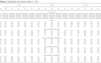
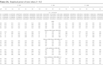
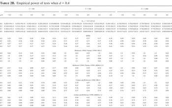
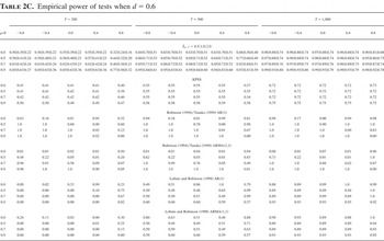
In Tables 1 and 2, the tests are constructed assuming a constant term in (1). Entries refer to empirical rejection frequencies at asymptotic critical values yielding a nominal size of 0.05. Standard normal critical values apply in each case apart from the KPSS test. All results are based on 10,000 replications.
Empirical size of tests when d = 0.0

Empirical power of tests when d = 0.2

Empirical power of tests when d = 0.4

Empirical power of tests when d = 0.6

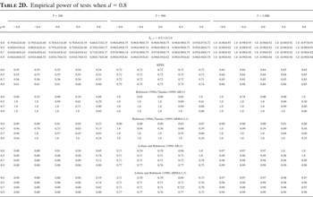
Empirical power of tests when d = 0.8

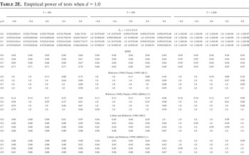
Empirical power of tests when d = 1.0

The empirical sizes for the tests are presented in Table 1. When c = 0.5, the

test can be seen to control size very well across the ARMA parameter space with the exception of when the autoregressive (AR) coefficient takes its largest value of ρ = 0.9. In this case its size generally exceeds 0.20 when T = 200. Increasing the sample size does, however, offset this effect reasonably quickly. When c = 1.0,

is only ever modestly oversized for ρ = 0.9 when T = 200 (though never above 0.10), and this problem is rapidly corrected as the sample size increases. For c = 2.0, there are no notable size distortions anywhere. This is entirely consistent with what we would expect in finite samples; other things being equal, the larger the AR root, the larger the value of c that will be required to correctly center the statistic.
The KPSS test has good size properties for small amounts of autocorrelation in ut but becomes oversized across all of the sample sizes for strong autocorrelation of an AR form, or large positive MA in small samples. The Robinson (1994)/Tanaka (1999) test assuming an AR(1) model for ut provides conservative sizes overall when the AR(1) model is correct but can be either badly oversized or undersized if the AR(1) model is incorrect and ARMA(1,1) is the true DGP. Those cases where the AR(1) model is misspecified are included to demonstrate the consequences of model misspecification in the parametric test. The Robinson (1994)/Tanaka (1999) test assuming an ARMA(1,1) model for ut is always based on a correctly specified model in these particular simulations, and therefore they provide reasonable size control, albeit being somewhat undersized for weak AR autocorrelation when T = 200. Of course, if the DGP for ut were of a higher order than ARMA(1,1) then the size properties of this test would be expected to be rather poor. The Lobato and Robinson (1998) tests can be seen to provide reasonable size control for negative values of θ, although with some undersizing for large values of ρ for T = 200. However, the AR(1) version has poor size properties for positive values of θ, with sizes approaching both zero and one in various areas of the parameter space. The ARMA(1,1) version does not suffer from this problem, although there is evidence of undersizing when T = 200 and there are also some sizes over 0.10 for ρ = 0 in the larger sample sizes. Despite this being a nonparametric test, the obvious implication of these results is that it is important to have a good approximating model from which to compute the bandwidth parameter for this test.
The corresponding empirical powers for the tests are reported in Tables 2A, 2B, 2C, 2D, & 2E. Recall that these are not size adjusted powers, and so comparisons across the tests need to be made keeping their relative size properties firmly in mind. It is clear that, for all c, the

test has power that increases with both d and T. For a given d and T, these powers also decline monotonically with c because the positive offset of the statistic declines as c increases. Our opinion is that the potential problems of controlling size when c = 0.5 are probably sufficient to outweigh its power advantages over c = 1.0, whereas we feel that the reverse is true on comparing c = 1.0 and c = 2.0. This leaves c = 1.0 as our compromise choice on which we base subsequent comparisons with the other tests.
The power of

is greater than that of KPSS almost everywhere when d is in the nonstationary region (for stationary values of d KPSS has the greater power unless the sample size is large). Hence, bearing in mind its superior control of size,

would appear to provide a very worthy competitor to KPSS as a test of short memory against nonstationary long memory and particularly in the I(1) case.
As might be expected, the powers of the Robinson (1994)/Tanaka (1999) tests are usually very good when the model for ut is specified correctly, although there are some curious exceptions in some parts of the ARMA parameter space for nonstationary values of d where the powers are extremely low. In fact, this test does not appear to be consistent for nonstationary d when ut is noise. We conjecture that, in such situations, prewhitening via AR/ARMA estimation is largely extracting the effects of nonstationary d (this certainly explains the results for d = 1). The Lobato and Robinson (1998) test using the ARMA(1,1) approximating model exhibits very good power properties for the largest sample size, T = 1,000, but is generally less powerful than

for the other sample sizes and is profoundly so when T = 200 and d is nonstationary.
In the case where (1) contains a linear trend term, simulations (not reported but available from the authors) show that the good size control properties of the

test continue to hold but with the absence of the modest oversizing seen previously. The size properties of the KPSS test also generally mimic those of the constant only case with the exception that a large positive MA component leads to much more serious oversizing in smaller samples. For the other four tests, their patterns of size largely carry over from the constant case but with almost every size being slightly smaller than before. The test powers are, overall, lower than in the constant case except for KPSS, which appears less affected by the presence of the trend.
In summary, then, we conclude from these simulations that

exhibits very good size control across a range of DGPs and sample sizes, to an extent not matched by the other tests in the comparison. For tests that rely on prewhitening, knowledge of the correct parametric model appears essential to avoid potentially severe size distortions. Similarly, bandwidth selection in the periodogram-based tests requires a good approximating parametric model to avoid finite-sample size distortion. Significantly, the size control of the new test does not appear to be achieved at the expense of being competitive in terms of power, particularly when nonstationary long memory alternatives are under consideration.
APPENDIX: Proofs
A.1. Proof of Theorem 1.
Similar to the definition of

, we define a statistic

based on the true zt, rather than

, as

where

and wj = 1/(j + 1) is defined for notational convenience. The proof uses (T − k)/T → 1 and the next four steps, which are proved in the following sequence of lemmas.
L1.

where

,
L2.

,
L3.

,
L4.

and

.
The result of Theorem 1 then follows by the continuous mapping theorem (CMT).
LEMMA 1. Under the conditions of Theorem 1,

.
Proof. Define the artificial autocovariances

, which clearly exist and are absolutely summable under the condition

. These γj provide useful bounds throughout the proof. Lemma 5 shows that the claimed expression for ω2 exists.
First note that

can be rewritten as

where

and

. In this notation

Substituting these expressions and rearranging gives

where

and δi,j = 1 for i = j and is zero otherwise. Applying the Beveridge–Nelson decomposition to gk,t,k−i(L) gives the martingale difference

where gk,t,k−i = gk,t,k−i(1). The existence of the ζk,t−1 process as a mean square limit follows from Lemma 6(i) with s = 0. The central limit theorem (CLT) is proved by showing
(a)

,
(b)

,
(c)

.
These results combine to give Lemma 1.
For (a) the martingale difference CLT is proved by showing
(i)

,

,
(ii)

.
Part (i) is shown by Lemma 6(iii) in Appendix A.3 (Technical Appendix),

To also show

, use mk,t = εtζk,t−1 to write

For any s ≥ 0

where κ4(.) denotes the (finite) fourth-order cumulant (see Hannan, 1970, Ch. 1, eqn. (5.1)), and Lemma 6(i) and (ii) provide the convergence of these sums. The martingale difference array (εt2 − 1)ζk,t−12 therefore has uniformly bounded variance (s = 0 in (A.3)), and hence the first term of (A.2) converges to zero in probability. Using (A.3), the variance of the second term of (A.2) can be written


Using the Cauchy–Schwarz (CS) inequality in (A.4) and then applying Lemma 6(i) and (ii) shows that (A.4) is bounded by

Now (T − k)−1k → 0, and the Cesaro sum disappears because

as s → ∞ by Lemma 5, and so it follows that (A.4) disappears as T → ∞. Rearranging sums in (A.5) gives

and this disappears by Lemma 6(i). This shows that

m as required.
For part (ii) it can be shown that for any ε > 0

and the preceding arguments for (i) show that E(mk,t4) is uniformly bounded for all k and t. Thus

as required.
We prove (b) by using

which gives


Clearly all terms have zero means, and so it is sufficient to show that their variances disappear. First (A.6) can be written

which has variance

and this disappears using k/T → 0 and Lemma 5. Similarly (A.8) can be written

which disappears in exactly the same way. Rearranging sums in (A.7) gives

which has variance

Using

(A.9) can be bounded by

which disappears by Cesaro summation because

as t → ∞.
To prove (c) we consider

where for s ≥ 0


where a = max(1,m4) and using

for all t. Substituting (A.11) and (A.12) into (A.10) and rearranging summations gives a bound for (A.10):

which disappears as T → ∞, and hence k → ∞, by the summability of |cj| and γs.
LEMMA 2. Under the conditions of Theorem 1,

.
Proof. We have

Under

we want to choose k so that

. Now

and

where γ is Euler's constant. Because

we thus have

and hence

, so that k must grow such that k/(T − k)1/2 [nrarr ] 0, i.e., k is at least O(T1/2). █
LEMMA 3. Under the conditions of Theorem 1,

.
Proof. The limiting variance has the form

because for j = 1,2,…,

where Hj is the jth harmonic number. So

where h0 = π2/6 and hj = | j|−1H| j| for j = ±1,±2,…. Note that

and

. The estimator based on zt is

and we define

We note that

and we show that each of these terms disappears asymptotically. First

for some a > 0. The bounds in the second inequality follow because

and

and the term involving the fourth cumulant is handled similarly, showing that

for some a uniformly in h ≤ 2l. Second

as l → ∞. Thus

as required. █
LEMMA 4. Under the conditions of Theorem 1,
(i)

,
(ii)

.
Proof. (i) The numerator of the statistic can be written

where

. We show that the last three terms disappear asymptotically. Note that

, and so

The second inequality follows by the vector CS inequality

. This bound also applies to

and

. Thus the second term on the right-hand side of (A.13) disappears as follows:

The third and fourth terms disappear similarly, which proves (i).
(ii) To show

, we write

in which
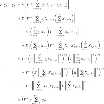
by application of (A.14). It thus follows that

for some a > 0. █
A.2. Proof of Theorem 2.
For d < 0.5 the statistic can be written as

It follows from Lemma 7 that there exists some J such that γj > 0 for all j ≥ J, so that

is positive for large enough k and has order

Now

where

and by CS inequality

so that

Also

which has order


The ratio

, the leading term in (A.16), therefore has order at least

and, because l/T1/2 → 0, the ratio diverges to +∞. To conclude from this that

diverges to +∞ we now argue that the second term in (A.16) converges in probability to +1.
In the numerator we have the term

To show that the first term disappears, we have by (A.15) that

whereas the denominator

has been shown to have a rate of divergence of at least k2d ln k, which is rate Td ln T with k = O(T1/2), and (T2d−1/2 ln T)/(Td ln T) → 0 for all d < ½. The second term disappears similarly because

. The disappearance of

in the denominator in (A.16) also follows by similar reasoning.
For d > 0.5 we first note that

so that for some c > 0

Next consider

for some 0 < ε < ½ (the inequality uses a + b ≥ a − |b| because b + |b| ≥ 0). Now

and clearly

uniformly for all j ≤ T1−ε. Using equation (22) of Tanaka (1999) and the CMT we obtain

and hence

where Fd−1 is given by Tanaka's equation (24) and φ by his equation (13). Also

uniformly for all j ≤ T1−ε. Thus,

and hence

uniformly for all j ≤ T1−ε. Therefore we write the first term in (A.19) as

Next we consider the second term in (A.19), which, using

for all j, can be written

Combining (A.20) and (A.21) in (A.19) gives

and then combining (A.22) and (A.18) gives

so that

diverges at least as fast as (T1/2 ln T)/(l1/2 ln l) as claimed. █
A.3. Technical Lemmas.
LEMMA 5. If

then

. Note that this also immediately implies

.
Proof. For any n > 0

LEMMA 6. For gk,t,k−i defined following (A.1),
(i) if 0 ≤ s ≤ k − 1,

,
(ii) if s ≥ k,

uniformly in t, and if k → ∞ as T → ∞ such that k/T → 0 then
(iii)

as T → ∞.
Proof. (i) For 0 ≤ s ≤ k − 1

where

and similarly

and so adding (A.23) and (A.24) gives the required bound.
(ii) For s ≥ k

and the bound follows similarly to (A.24).
(iii) The sum can be written

where

. We can validly define

where

and xT,∞ exists by part (i). We now show that

where

. To do this, first write

Now

where

Substituting (A.28) into (A.27) gives

as required for (A.26). Combining (A.25) and (A.26) shows

as T → ∞ by Cesaro summation, because Lemma 5 implies that ct → 0 as t → ∞.
It is therefore left to show that

as T → ∞. Now substituting for gk,∞,k−i2 and f∞,j−i with some rearrangement gives

where

. Thus

The second term on the right-hand side is bounded by

, which, in view of Lemma 5, clearly disappears as k → ∞. So it remains to consider the first term, which can be seen to be bounded by 2ωrk1/2 + rk where

and

. Rearrangement of the second term shows that it is bounded by

, which disappears as k → ∞ by Lemma 5. The first term is bounded by

which disappears for k → ∞ as cj is absolutely summable. Thus rk → 0 and

. █
LEMMA 7. Under the conditions of Theorem 2 with 0 < d < ½ the autocovariance function of zt, denoted γh, satisfies

where γu,j denotes the autocovariance function of ut.
Proof. The proof follows that of Theorem 13.2.2 of Brockwell and Davis (1991). We have

where γx,j is the autocovariance function of the fractional noise process (1 − L)dxt = et where et is unit variance white noise. We can write

The second of these terms satisfies

which disappears as h → ∞ because

implies that

. Next,

uniformly in j for | j| ≤ h1−2d because 1 − 2d < 1, and so the first term in (A.29) satisfies

as required. █