2. The governing equations

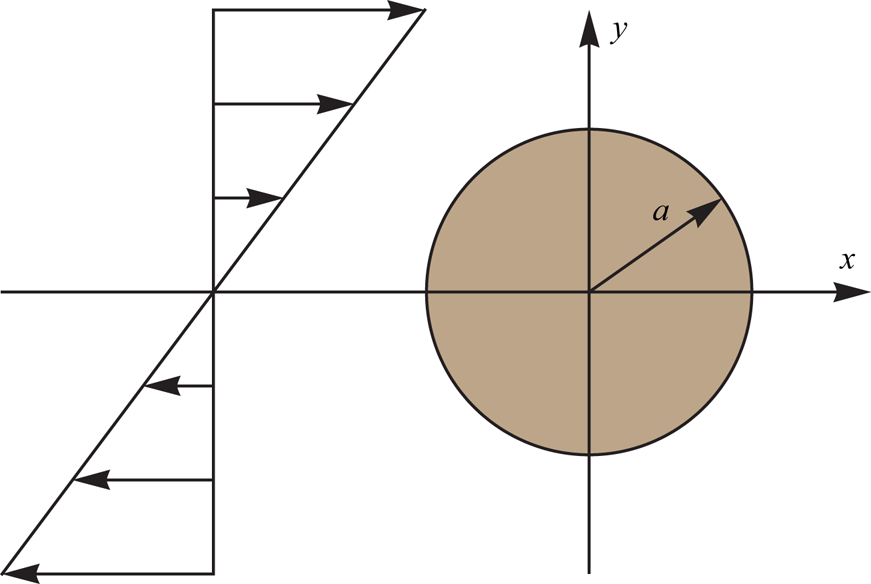
Figure 1 describes an initially non-buoyant spherical drop (radius a) of one fluid positioned at the origin of a coordinate system and submerged in another fluid. Let both fluids be immiscible, incompressible, Newtonian and under creeping flow conditions. Far away from the drop, the external fluid experiences a nonlinear cubic shear flow (in two directions), defined in Cartesian coordinates (x, y, z) as

(2.1)\begin{gather}{v_x} = Ay + B{y^3},\end{gather}

(2.2)\begin{gather}{v_y} = Cx + B{x^3},\end{gather}

(2.3)\begin{gather}{v_z} = 0,\end{gather}

(2.4)\begin{gather}p = 6\mu Bxy + K.\end{gather}

Here, p is the pressure, $\mu$ is the viscosity of the external fluid and K is an arbitrary constant. Note that quadratic terms are missing in order to maintain an odd velocity profile around the origin. The constants A, B and C can attain positive, negative or zero values, and if B = C = 0, and A > 0, the familiar simple (linear) shear flow, described in figure 1, is recovered. Furthermore, the constants of the terms with the cubic powers must be the same, otherwise the Stokes equations cannot be fulfilled. Similar to simple shear flow, this nonlinear shear flow possesses angular deformation and rotation but not linear deformation.

Figure 1.

A spherical drop in a simple (linear) shear flow (A > 0, B = C = 0).

In spherical coordinates (r, θ, ϕ), with 0 ≤ θ ≤ π being the polar angle and 0 ≤ ϕ < 2π the azimuth angle, the undisturbed motion, given by (2.1)–(2.4), reads

(2.5)\begin{gather}{v_r} = {\textstyle{1 \over 2}}(A + C)r{\sin ^\textrm{2}}\theta \sin (\textrm{2}\phi ) + {\textstyle{1 \over 2}}B{r^3}{\sin ^\textrm{4}}\theta \sin (\textrm{2}\phi ),\end{gather}

(2.6)\begin{gather}{v_\theta } = {\textstyle{1 \over 2}}(A + C)r\cos \theta \sin \theta \sin (2\phi ) + {\textstyle{1 \over 2}}B{r^3}\cos \theta {\sin ^3}\theta \sin (2\phi ),\end{gather}

(2.7)\begin{gather}{v_\phi } = {\textstyle{1 \over 2}}r\sin \theta [ - A + C + (A + C)\cos (2\phi )] + B{r^3}{\sin ^3}\theta \cos (2\phi ),\end{gather}

(2.8)\begin{gather}p = 3\mu B{r^2}{\sin ^2}\theta \sin (2\phi ) + K.\end{gather}

The Stokes equations, outside and inside the drop, together with the appropriate boundary conditions, suggest a problem which is governed by four dimensionless parameters. These are: the capillary number (Ca), the viscosity ratio (λ), the linear velocity ratio (G) and the nonlinear intensity of the flow (E)

(2.9)\begin{gather}Ca = \frac{{\mu Aa}}{\sigma },\end{gather}

(2.10)\begin{gather}\lambda = \frac{{{\mu _{in}}}}{\mu },\end{gather}

(2.11)\begin{gather}G = \frac{C}{A},\end{gather}

(2.12)\begin{gather}E = \frac{{B{a^2}}}{A}.\end{gather}

Here, $\mu$ and $\mu_{in}$ are the external and internal viscosities, respectively, a is the initial radius of the spherical drop and σ is the surface tension. Note that since the constants A, B and C can be positive, negative or zero, this suggests the same for Ca, G and E.

From now on and in what follows, we non-dimensionalize the lengths with the initial drop radius (a), the velocities with the characteristic linear velocity (U = Aa) and the pressures and viscous stresses with the characteristic external stress ($\mu A$). A general solution the Stokes equations, in spherical coordinates, was suggested by Lamb (Reference Lamb1945), see also Happel & Brenner (Reference Happel and Brenner1983) and Zapryanov & Tabakova (Reference Zapryanov and Tabakova1999). For the internal flow have

(2.13)\begin{gather}{\boldsymbol{v}_{in}} = \sum\limits_{n = 1}^\infty {\left[ {\frac{{(n + 3){r^2}\boldsymbol{\nabla }{p_{n,in}}}}{{2\lambda (n + 1)(2n + 3)}} - \frac{{nr\boldsymbol{e}_r{p_{n,in}}}}{{\lambda (n + 1)(2n + 3)}} + \boldsymbol{\nabla }{\Phi_{n,in}} + \boldsymbol{\nabla } \times (r\boldsymbol{e}_r{\chi_{n,in}})} \right]} ,\end{gather}

(2.14)\begin{gather}{p_{in}} = {p_0} + \sum\limits_{n = 1}^\infty {{p_{n,in}}} ,\end{gather}

(2.15)\begin{gather}{p_{n,in}} = {r^n}\sum\limits_{m = 0}^n {P_n^m(\eta )[{a_{n,m}}\cos (m\phi ) + {b_{n,m}}\sin (m\phi )]} ,\end{gather}

(2.16)\begin{gather}{\varPhi _{n,in}} = {r^n}\sum\limits_{m = 0}^n {P_n^m(\eta )[{c_{n,m}}\cos (m\phi ) + {d_{n,m}}\sin (m\phi )]} ,\end{gather}

(2.17)\begin{gather}{\chi _{n,in}} = {r^n}\sum\limits_{m = 0}^n {P_n^m(\eta )[{e_{n,m}}\cos (m\phi ) + {f_{n,m}}\sin (m\phi )]} .\end{gather}

And by replacing n with $- (n + 1)$, we arrive at the external flow expressions

(2.18)\begin{gather}{\boldsymbol{v}_{out}} = {\boldsymbol{v}_\infty } + \sum\limits_{n = 1}^\infty {\left[ { - \frac{{(n - 2){r^2}\boldsymbol{\nabla }{p_{n,out}}}}{{2n(2n - 1)}} + \frac{{(n + 1)r\boldsymbol{e}_r{p_{n,out}}}}{{n(2n - 1)}} + \boldsymbol{\nabla }{\Phi_{n,out}} + \boldsymbol{\nabla } \times (r\boldsymbol{e}_r{\chi_{n,out}})} \right]} ,\end{gather}

(2.19)\begin{gather}{p_{out}} = {p_\infty } + \sum\limits_{n = 1}^\infty {{p_{n,out}}} ,\end{gather}

(2.20)\begin{gather}{p_{n,out}} = {r^{ - n - 1}}\sum\limits_{m = 0}^n {P_n^m(\eta )[{a_{ - n - 1,m}}\cos (m\phi ) + {b_{ - n - 1,m}}\sin (m\phi )]} ,\end{gather}

(2.21)\begin{gather}{\varPhi _{n,out}} = {r^{ - n - 1}}\sum\limits_{m = 0}^n {P_n^m(\eta )[{c_{ - n - 1,m}}\cos (m\phi ) + {d_{ - n - 1,m}}\sin (m\phi )]} ,\end{gather}

(2.22)\begin{gather}{\chi _{n,out}} = {r^{ - n - 1}}\sum\limits_{m = 0}^n {P_n^m(\eta )[{e_{ - n - 1,m}}\cos (m\phi ) + {f_{ - n - 1,m}}\sin (m\phi )]} .\end{gather}

Here, v is the velocity, v_∞ and p_∞ are the velocity vector and pressure of the unperturbed motion, p ₀ is the internal pressure in the absence of flow, e_r is the unit vector in the radial direction and the subscripts in and out represent inside and outside the drop, respectively. The functions p_n, Φ_n and χ_n are solid spherical harmonics with $P_n^m(\eta )$ being the associated Legendre polynomials of degree n and order m, and the usual substitution in spherical coordinates (η = cosθ) has been made. The constants in (2.15)–(2.17) and (2.20)–(2.22) are to be evaluated according to the usual boundary conditions suggested by the literature.

The no slip condition requires equal velocities at the interface (r = 1). Furthermore, in a stationary drop the normal velocities also vanish:

(2.23)\begin{gather}{v_{r,out}} = {v_{r,in}} = 0,\end{gather}

(2.24)\begin{gather}{v_{\theta ,out}} = {v_{\theta ,in}},\end{gather}

(2.25)\begin{gather}{v_{\phi ,out}} = {v_{\phi ,in}}.\end{gather}

Newton's third law of motion requires the normal and tangential stresses of the two fluids to be balanced at the interface (r = 1). For the tangential stress we have

(2.26)\begin{gather}{\tau _{r\theta ,out}} = {\tau _{r\theta ,in}},\end{gather}

(2.27)\begin{gather}{\tau _{r\phi ,out}} = {\tau _{r\phi ,in}}.\end{gather}

According to the method for solving this type of problem, (2.13)–(2.27) are sufficient to obtain the spherical solution O(Ca ⁰). This zeroth-order solution can then be substituted into the normal stress balance at the interface to obtain the first-order, O(Ca ¹), deformed shape

(2.28)\begin{equation}{p_{in}} - {p_{out}} + {\tau _{rr,out}} - {\tau _{rr,in}} = \frac{1}{{Ca}}\left( {\frac{1}{{{R_1}}} + \frac{1}{{{R_2}}}} \right),\end{equation}

where R ₁ and R ₂ are the principal radii of curvature of the surface.

3. The undisturbed motion

In order to better understand this physical situation, it is worthwhile to describe first the behaviour of the undisturbed motion, that is, the flow in the absence of the drop. Since the undisturbed motion is an incompressible two-dimensional flow, we can easily define and obtain for it a dimensionless streamfunction

(3.1)\begin{gather}{v_x} ={+} \frac{{\partial \psi }}{{\partial y}} = y + E{y^3},\end{gather}

(3.2)\begin{gather}{v_y} ={-} \frac{{\partial \psi }}{{\partial x}} = Gx + E{x^3},\end{gather}

(3.3)\begin{gather}\psi = \frac{1}{2}({y^2} - G{x^2}) + \frac{E}{4}({y^4} - {x^4}).\end{gather}

Note that v_x vanishes at y = 0 or $y ={\pm} i/\sqrt E $, while v_y vanishes at x = 0 or $x ={\pm} i\sqrt {G/E} $.

In terms of the strain rate tensor ($\boldsymbol{\varGamma}$) and the vorticity tensor ($\boldsymbol{\varOmega}$), the only non-vanishing components are

(3.4)\begin{gather}{\varGamma _{xy}} = {\varGamma _{yx}} = {\textstyle{1 \over 2}}[(1 + G) + 3E({x^2} + {y^2})],\end{gather}

(3.5)\begin{gather}{\varOmega _{xy}} ={-} {\varOmega _{yx}} = {\textstyle{1 \over 2}}[(G - 1) + 3E({x^2} - {y^2})].\end{gather}

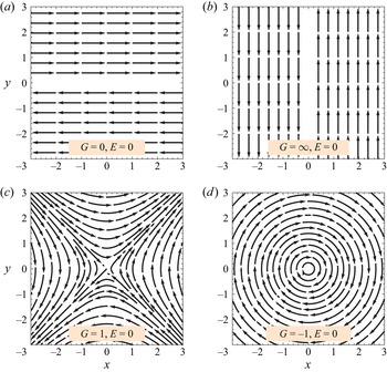
Thus, for a linear shear flow (E = 0), if G = 0 we have the familiar simple shear flow in the x-direction with both angular deformation and rotation of the same magnitude, if G = 1 there is only angular deformation and if G = −1 there is only rotation. In a nonlinear shear flow (E ≠ 0), there will be always angular deformation and rotation simultaneously.

Figure 2 shows the velocity vector of the unperturbed motion for the case where the shear flow is linear (E = 0). Four G cases are described: the familiar simple shear flow in which the velocity is in the x-direction (G = 0) or in the y-direction (G = ∞); a positive case (G = 1), where observing at an angle of ϕ = 45° suggests an extensional flow; and finally, a negative case (G = −1), where the fluid rotates clockwise.

Figure 2.

The undisturbed motion in a linear (E = 0) shear flow.

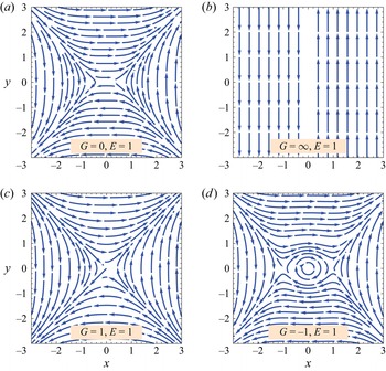
The undisturbed motion with a positive nonlinear intensity (E = 1) is described in figure 3. The case G = ∞ is similar to the linear flow in the y-direction of figure 2, since then the linear velocity term is much larger than the nonlinear term. The remaining three cases are all similar in form, with the case G = −1 also showing a clockwise circulation. This circulation increases in size as E decreases, until the image of the linear case (G = −1, E = 0) is recovered.

Figure 3.

The undisturbed motion in a positive nonlinear (E > 0) shear flow.

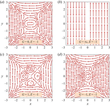
Probably the most interesting undisturbed motion case is shown in figure 4, where the nonlinear intensity of the flow is negative (E = −1). Once again, the case G = ∞ is similar to the linear flow in the y-direction of figure 2, since then the linear velocity term is much larger than the nonlinear term. The third case (G = 1) is fascinating, since, if observing it from an angle of ϕ = ±45°, it mimics a drop in an extensional flow, with the familiar internal circulations, despite the fact that there is no drop at all! Figures 2–4 show just a few possibilities for the undisturbed motion. Many more interesting streamline shapes can be obtained by exploring different combinations of G and E, as a result of the inclusion of nonlinear terms to the velocity field, which among other features, also suggests up to eight stagnation points, besides the one at the origin which always is present. These are located at: (0, 0); (0, ${\pm} i/\sqrt E $); (${\pm} i\sqrt {G/E} $, 0); (${\pm} i\sqrt {G/E} $, ${\pm} i/\sqrt E $); and (${\pm} i\sqrt {G/E} $, ${\mp} i/\sqrt E $).

Figure 4.

The undisturbed motion in a negative nonlinear (E < 0) shear flow.

4. The disturbed motion

The flow in the presence of a spherical drop, corresponding to the limit of Ca = 0, can be obtained by solving the Stokes equations with the appropriate boundary conditions, as suggested by (2.13)–(2.27). It appears that, if the linear case (E = 0) can be satisfied with n = 1 and 2, our nonlinear problem requires n = 1, 2, 3 and 4. With the assistance of the Mathematica software, the following analytical expressions for the coefficients in the solid harmonics were obtained. For the external flow we have

(4.1)\begin{gather}{b_{ - 3,2}} ={-} \frac{{(2 + 5\lambda )(1 + G)}}{{6(1 + \lambda )}} - \frac{{\lambda E}}{{(1 + \lambda )}},\end{gather}

(4.2)\begin{gather}{b_{ - 5,2}} ={+} \frac{{(2 + 9\lambda )E}}{{75(1 + \lambda )}},\end{gather}

(4.3)\begin{gather}{d_{ - 3,2}} ={-} \frac{{\lambda (1 + G)}}{{12(1 + \lambda )}} + \frac{{(2 - 5\lambda )E}}{{42(1 + \lambda )}},\end{gather}

(4.4)\begin{gather}{d_{ - 5,2}} ={+} \frac{{\lambda E}}{{150(1 + \lambda )}},\end{gather}

(4.5)\begin{gather}{e_{ - 4,2}} ={+} \frac{{(1 - \lambda )E}}{{30(5 + 2\lambda )}}.\end{gather}

While the coefficients of the internal flow are

(4.6)\begin{gather}{b_{2,2}} ={+} \frac{{7\lambda (1 + G)}}{{4(1 + \lambda )}} + \frac{{7\lambda E}}{{2(1 + \lambda )}},\end{gather}

(4.7)\begin{gather}{b_{4,2}} ={-} \frac{{11\lambda E}}{{60(1 + \lambda )}},\end{gather}

(4.8)\begin{gather}{d_{2,2}} ={-} \frac{{(1 + G)}}{{8(1 + \lambda )}} - \frac{E}{{4(1 + \lambda )}},\end{gather}

(4.9)\begin{gather}{d_{4,2}} ={+} \frac{E}{{120(1 + \lambda )}},\end{gather}

(4.10)\begin{gather}{e_{1,0}} ={-} \frac{{(1 - G)}}{2},\end{gather}

(4.11)\begin{gather}{e_{3,2}} ={+} \frac{{7E}}{{60(5 + 2\lambda )}},\end{gather}

where the rest of the coefficients vanish.

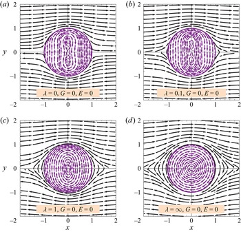
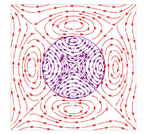
Figure 5 represents the velocity vector of the disturbed motion, in the z = 0 plane, for the familiar simple (linear) shear flow (E = 0, G = 0), where the velocity of the unperturbed motion is in the x-direction only. This case has been extensively explored by Bartok & Mason (Reference Bartok and Mason1958). Four viscosity ratios are presented, from a bubble or an inviscid drop (λ = 0) up to a solid sphere (λ = ∞). When λ = 0, the external streamlines are open while the internal streamlines suggest the familiar ‘8’ shape combined with oval streamlines. A similar picture is observed for the λ = 0.1 case, except that the external streamlines are closed. For low values of λ, where the ‘8’ shape exists, the drop contains two additional stagnation points, besides the one at the origin. At z = 0, these are located at ϕ = 90° and ϕ = 270° and at $r = \sqrt {(1 - 2\lambda )/5} $ suggesting that the ‘8’ shape can be established only if λ < 1/2 (Bartok & Mason Reference Bartok and Mason1958). Next is λ = 1, where the two phases are of equal viscosity, and where the internal streamlines are everywhere oval in shape. Finally, when λ = ∞, the drop becomes a solid sphere rotating clockwise at an angular velocity ω = −1/2 in accordance with the literature. In general, the angular velocity of a solid sphere in this problem is $\omega ={-} (1 - G)/2$ and independent of E.

Figure 5.

The disturbed motion in a linear (E = 0) shear flow, with G = 0, as a function of λ.

Another interesting feature of the flow field is the location of surface stagnation points. At the surface of the drop (r = 1) and at the z = 0 plane (η = 0), v_r = v_θ = 0, and the condition for a vanishing v_ϕ leading to a stagnation point can be expressed as

(4.12)\begin{equation}\phi ={\pm} \frac{1}{2}{\cos ^{ - 1}}\left[ {\frac{{10(1 - G)(1 + \lambda )(5 + 2\lambda )}}{{10(1 + G)(5 + 2\lambda ) + 7E(20 + 11\lambda )}}} \right] + n{\rm \pi} ,\end{equation}

where n is an integer. It follows that, for the cases described in figure 5 (G = E = 0), only the inviscid drop (λ = 0) predicts real azimuthal angles which are located at ϕ = 0° and ϕ = 180°. The inviscid drop is also the only case in figure 5 suggesting no closed external streamlines, an important issue when dealing with mass transfer problems around such a drop.

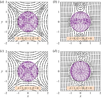
Next, in figure 6, we continue with the velocity vector in a linear shear flow (E = 0) at the z = 0 plane, but with a positive linear velocity ratio (G > 0). Two viscosity ratios (λ = 0, 1) and two linear velocity ratios (G = 1, 10) are described. For the two G = 1 cases, and if observing at ϕ = ±45°, an extensional flow is produced (see figure 2, G = 1) suggesting similar streamlines shapes for all values of λ. However, when $G \gg 1$, the external flow moves towards a simple shear flow in the in the y-direction (see figure 2, G = ∞), where, similar to the familiar simple shear flow (figure 5), the shape of the internal streamlines strongly depends on λ. The surface stagnation points in figure 6 can be easily located according to (4.12). The case G = 1 is unique since it suggests the simple expression of $\phi = ({\pm} 1/4 + n){\rm \pi}$, which is independent of λ or E. The angular velocity of a solid sphere (λ = ∞) is $\omega ={-} (1 - G)/2$ and independent of E. That is, for G = 1 it vanishes, while for G > 1 it results in ω > 0 or a counter-clockwise rotation.

Figure 6.

The disturbed motion in a linear (E = 0) shear flow, with G > 0, as a function λ.

Figures 5 and 6 suggests that, for the linear case (E = 0), the internal flow within the drop contains zero, two or four stagnation points, besides the one at the origin. The first pair is located at ϕ = 0° and ϕ = 180°, and its distance from the origin is

(4.13)\begin{equation}r = \sqrt {\frac{{5 + 2\lambda + (1 - 2\lambda )G}}{{5(1 + G)}}} .\end{equation}

While the next pair is positioned at ϕ = 90° and ϕ = 270°, and at

(4.14)\begin{equation}r = \sqrt {\frac{{1 - 2\lambda + (5 + 2\lambda )G}}{{5(1 + G)}}} .\end{equation}

It follows that, for G = 1, these two pairs are at equal distance $r = \sqrt {3/5} = 0.775$ from the origin and independent of λ. When λ = 0 and G = 10, the first pair is at ${r = \sqrt{3/11} = 0.522}$, and the second one at $r = \sqrt{51/55} = 0.963$. However, if λ = 1 and G = 10, the first pair does not exist (r is imaginary), and the second one does not exist either (r > 1).

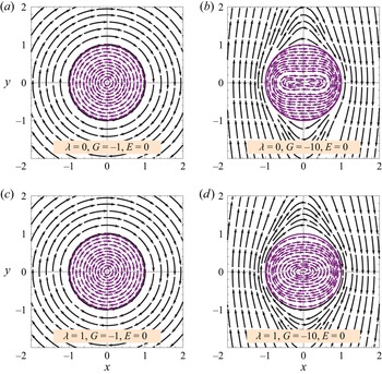
Figure 7 finalizes our linear (E = 0) findings, by plotting the velocity vector at the z = 0 plane, with a negative velocity ratio (G < 0). As in figure 6, two viscosity ratios (λ = 0, 1) and two linear velocity ratios (G = −1, −10) are presented. The case E = 0 and G = −1 is unique since, in the entire space, all velocity components vanish except v_ϕin = v_ϕout = −rsinθ, independent of λ. That is, the drop rotates clockwise like a solid particle at an angular velocity ω = −1. As G becomes more negative, the external streamlines change their configuration from circles towards ellipse-like shapes and, if $\textrm{|}G\textrm{|} \gg 1$, we approach a simple shear flow in the y-direction but in opposite direction to the one presented in figure 2. When G < 0 (E = 0), (4.12) predicts no stagnation points at the surface of the drop. Figure 7 shows that, if G < 0 (G ≠ −1), the internal circulation is a strong function of λ, predicting once again oval shape streamlines with or without the ‘8’ structure (which now lies down). The internal stagnation points, besides the one at the origin, can be obtained from (4.13) and (4.14), where it is clear that, if G = −1, they do not exist as the denominator vanishes. For the G = −10 cases described here, only λ = 0 predicts internal stagnation points and only one pair located at ϕ = 0° and ϕ = 180° at a distance r = 1/3 from the origin.

Figure 7.

The disturbed motion in a linear (E = 0) shear flow, with G < 0, as a function λ.

Now that we are familiar with the disturbed linear (E = 0) behaviour, we can move forward and explore nonlinear (E ≠ 0) shear flows in the presence of a drop. For a spherical drop (Ca = 0), the problem is governed by three dimensionless numbers (λ, G, E), and the number of combinations is extremely large. To reduce the number of figures, we explore the case λ = 1 only, at three different linear velocity ratios (G = 0, 1, −1). All forthcoming velocity vector plots are shown at the z = 0 plane.

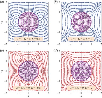
The first nonlinear plot of the disturbed motion is presented in figure 8, where λ = 1, G = 0 and E adopts positive and negative values. In the first case (E = 0.1), the nonlinear intensity of the flow is weak, and since G = 0, the flow behaviour is not far from the familiar simple shear flow (G = 0, E = 0). Some differences are observed in the external flow, where the present case has stagnation points at ϕ = 0°, ϕ = 180° and r = 1.15, whereas the linear case has not. On the other hand, the internal streamlines are oval, with no stagnation points apart from the origin, as in the familiar simple shear flow case λ = 1. No stagnation points are present at the surface of the drop. Next, we increase the nonlinear intensity (E = 1) and dramatic changes occur everywhere. Now, the external flow does not contain stagnation points, but the surface of the drop does (ϕ = ±30.4°, ±149.6°). Inside the drop, four additional stagnation points are created, at the usual azimuthal angles. The first pair is located at ϕ = 0° and 180° with r = 0.874, while for the second one we have ϕ = 90° and 270° with r = 0.547.

Figure 8.

The disturbed motion in a nonlinear (E ≠ 0) shear flow, with λ = 1 and G = 0, as a function of E. Blue: E > 0; red E < 0.

When E < 0, and if G = 0, the undisturbed motion has stagnation points (besides the origin) at x = 0, $y ={\pm} i/\sqrt E $. As |E| increases and the flow becomes more nonlinear, this stagnation point moves towards the origin. For E = −1/2, this point is located at $(0, \pm \sqrt 2 )$ and its location, if the flow is disturbed, is not far away from it (0, ±1.39). The direction of the flow above and below of this point is reversed, as can be seen in the first E < 0 case of figure 8. No stagnation points are predicted at the surface of the drop or inside the drop, except at the origin. As |E| continues to increase, ${\pm} i/\sqrt E $ approaches the origin, and the stagnation point in the external fluid, where the flow changes direction, does not exist anymore. This is illustrated in the last example of figure 8 where four stagnation points are created at the surface of the drop (ϕ = ±56.3°, ±123.7°) and four others within the drop (ϕ = 0°, 180° and r = 0.522; ϕ = 90°, 270° and r = 0.828).

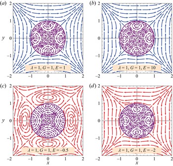
The next nonlinear disturbed motion plot is shown in figure 9, where λ = 1 and G = 1 for all cases. The two positive nonlinear intensities E = 1 and E = 10, are not only similar in form, but they also behave as in the linear case (λ = 1, G = 1, E = 0) in figure 6. That is, if observing from an angle ϕ = ±45°, we have an extensional flow. The only difference between the cases is the volumetric flow rate which increases with an increase in E. Stagnation points are not present in the external flow; however, they are present at the surface of the drop (ϕ = ±45°, ±135°), and within the drop (ϕ = 0°, 90°, 180°, 270°). It appears that, for a constant λ and if G = 1, all these four points are located at equal distances from the origin. For λ = 1 we have: E = 0, $r = \sqrt {3/5} = 0.775$; E = 1, r = 0.741; E = 10, r = 0.716; E = ∞, r = 0.711. Thus, the distance of the internal stagnation points from the origin slightly decreases as E increases.

Figure 9.

The disturbed motion in a nonlinear (E ≠ 0) shear flow, with λ = 1 and G = 1, as a function of E. Blue: E > 0; red E < 0.

The two cases at the bottom of figure 9 correspond to λ = 1, G = 1 and E < 0. Since both E < 0 and G/E < 0, the undisturbed motion predicts eight stagnation points besides the one at the origin. These are located at: (0, ${\pm} i/\sqrt E $); (${\pm} i\sqrt {G/E} $, 0); (${\pm} i\sqrt {G/E} $, ${\pm} i/\sqrt E $); and (${\pm} i\sqrt {G/E} $, ${\mp} i/\sqrt E $). The stagnation points move towards the origin as |E| increases. In the first case, G = 1 and E = −1/2, the first two pairs are located at (0, ${\pm} \sqrt 2 $) and (${\pm} \sqrt 2 $, 0) and their position in the disturbed motion is not far from (0, ±1.35) and (±1.35, 0). Around these stagnation points, circulations are formed. In addition, four stagnation points in the external fluid can be observed at (ϕ = ±45°, ±135°, r = 1.78) to support such complex structure. As |E| increases and the flow becomes more nonlinear, as can be seen in the last example of figure 9 (E = −2), these eight stagnation points just described move towards the origin and disappear in the external fluid. Both E < 0 cases suggest four stagnation points at the surface of the drop (ϕ = ±45°, ±135°, r = 1), and another four (besides the origin) within the drop (ϕ = 0°, 90°, 180°, 270°). Those within the drop move toward the surface as |E| increases from E = 0 (E = 0, $r = \sqrt {3/5} = 0.775$; E = −0.5, r = 0.867; E = −0.645, r = 0.9997). These points disappear in the range −1 < E < −0.646, and emerge once again at E < −1 (E = −1, r = 0; E = −2, r = 0.664; E = −10, r = 0.706; E = −∞, r = 0.711).

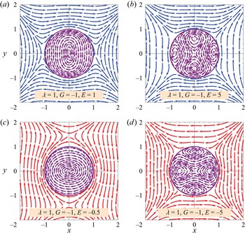
The last undisturbed motion is presented in figure 10, where once again λ = 1 but with a negative linear velocity ratio (G < 0). The first positive nonlinear intensity case (E = 1) should be compared with its equivalent undisturbed motion in figure 3 (G = −1, E = 1). The external fluid contains two stagnation points (ϕ = 0°, 180°, r = 1.07); however, the surface of the drop and the internal fluid (except the origin) do not. As E increases, as shown in the second case (E = 5), the stagnation points in the external fluid disappear, yet they emerge at the surface of the drop (ϕ = ±37.5°, ±142.5°) and within the drop (ϕ = 0°, 180° and r = 0.798; ϕ = 90°, 270° and r = 0.612). For λ = 1 and G = −1, the first pair (ϕ = 0°, 180°) appears if E > 1.29 from r = 1 and reaches r = 0.711 at E = ∞, while the second pair (ϕ = 90°, 270°) appears when E > 1.33 from r = 0 and approaches also r = 0.711 at E = ∞.

Figure 10.

The disturbed motion in a nonlinear (E ≠ 0) shear flow, with λ = 1 and G = −1, as a function of E. Blue: E > 0; red E < 0.

The next two cases correspond to negative nonlinear intensities (E < 0). In the first one (E = −0.5), the external flow contains two stagnation points (ϕ = 90°, 270°, r = 1.43), not far from those of the undisturbed motion (0, ${\pm} \sqrt 2 $). Yet, both the surface of the drop and the internal fluid (besides the origin) do not contain stagnation points. As |E| increases and the flow becomes more nonlinear (E = −5), the situation is reversed. Stagnation points in the external fluid disappear, but appear at the surface (ϕ = ±52.5°, ±127.5°) and within the drop (ϕ = 0°, 180° and r = 0.612; ϕ = 90°, 270° and r = 0.798). For λ = 1 and G = −1, the first pair (ϕ = 0°, 180°) appears if E < −1.33 from r = 0 until r = 0.711 at E = −∞, while the second pair (ϕ = 90°, 270°) appears if E < −1.29 from r = 1 and approaches r = 0.711 at E = −∞. Thus, one concludes that, if the present situation (E = −5) is rotated at ϕ = 90°, the previous internal findings (E = 5) are recovered.

5. Deformation of the drop

So far, the velocity profiles outside and inside a spherical drop, representing the O(Ca ⁰) solution, are available to us. The normal viscous stresses can be evaluated from Newton's viscosity law, and the pressures from (2.14) and (2.19). These can be then substituted into the normal stress balance, (2.28), that has not been applied yet, to obtain the O(Ca ¹) shape of the deformed drop. Let the distance from the origin to the surface of the deformed drop be

(5.1)\begin{equation}R(\theta ,\phi ) = 1 + Ca\,f(\theta ,\phi ),\end{equation}

Where, according to Landau & Lifshitz (Reference Landau and Lifshitz1987), the shape function f(θ, ϕ) is connected to the principal radii of curvature, obtained from the normal stress balance, as follows:

(5.2)\begin{equation}\frac{1}{{{R_1}}} + \frac{1}{{{R_2}}} = 2 - Ca(2f + {\nabla ^2}f).\end{equation}

In (5.2), the Laplacian operator should be in spherical coordinates. After some algebraic manipulation, the expression the shape of the deformed drop is given by

(5.3)\begin{align} R &= 1 + Ca(1 + G)\dfrac{{(16 + 19\lambda )}}{{16(1 + \lambda )}}(1 - {\eta ^2})\sin (2\phi )\nonumber\\ & \quad + CaE\dfrac{{7[28 + 41\lambda - {\eta ^2}(16 + 17\lambda )]}}{{240(1 + \lambda )}}(1 - {\eta ^2})\sin (2\phi ). \end{align}

When G = E = 0, the shape of the familiar (linear) simple shear flow is recovered. The maximum and minimum semi-axes in the z = 0 (η = 0) plane can be found by solving $\partial R/\partial \phi = 0$. As expected, these are located at the principal axes of extension or compression (ϕ = ±45°, ±135°), for both linear and nonlinear shear flows. The expression presented here for the shape of the drop is valid for a slightly deformed drop with λ = O(1), G = O(1), E = O(1) and $Ca \ll 1$. For a simple shear flow, Taylor (Reference Taylor1934) showed that small deformations are also possible for highly viscous drops $\lambda \gg 1$ with Ca = O(1) where the major axis of the deformed drop is positioned in the direction of the flow. In section 6 we shall discuss high viscosity drops.

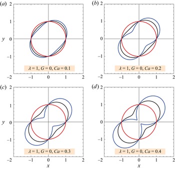
Figure 11 describes the shape of a drop with λ = 1 and G = 0 at different values of Ca. Each figure contains the linear case (E = 0) as well as positive and negative nonlinear intensities (E = ±1). As expected, the deformation of the drop increases as Ca increases. When the nonlinear intensity is positive (E = 1), the drop is more elongated than the linear case, and when it is negative (E = −1), the drop is less elongated than the linear case. This is also expressed by the familiar centre pinching or peanut shape, which for E > 0 it is developed at a lower Ca than the linear case, and for E < 0 it is not developed at all as a result of extremely small deformations. At ϕ = 0°, 90°, 180° and 270°, the distance of the surface to the origin is R = 1.

Figure 11.

The shape of a drop with λ = 1 and G = 0 as a function of Ca. Black: E = 0; blue: E = 1; red E = −1.

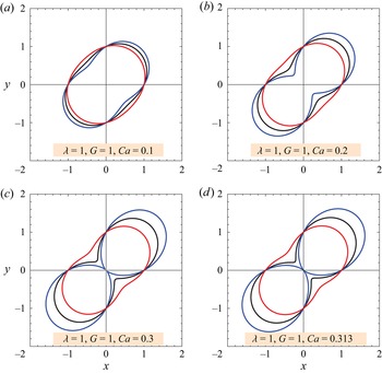
In figure 12 we continue to describe the shape of the same drop (λ = 1), but this time the linear velocity ratio is G = 1. Once again, each figure accommodates three different nonlinear intensities (E = 0, ±1). It appears that the same behaviour observed in the previous case (G = 0) occurs here (G = 1) as well. That is, the deformation of the drop increases with an increase in E. Note that the influence of G on the shape of the drop takes place only in the second (linear) term on the right-hand side of (5.3). It is clear from the shape expression that larger deformations are to be expected when G = 1 (figure 12) than when G = 0 (figure 11). This is also reflected by the evidence that, contrary to figure 11, this time even the E = −1 case shows the peanut shape. The last case had to be stopped at Ca = 0.313 as, beyond that, no steady shape was possible for E = 1.

Figure 12.

The shape of a drop with λ = 1 and G = 1 as a function of Ca. Black: E = 0; blue: E = 1; red E = −1.

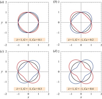
Finally, in figure 13 we portray the deformation of the drop when λ = 1 and G = −1. The case G = −1 is unique since the second (linear) term on the right-hand side of the shape (5.3) vanishes. Furthermore, for the linear case (E = 0), even the last term on the right-hand side vanishes, suggesting that no deformation is possible since the unperturbed flow contains vorticity but not angular deformation. The two nonlinear situations of E = ±1 offer the same deformation but at different orientations. For E = 1, the drop is aligned at ϕ = 45°, while for E = −1 at ϕ = −45°; however, it is possible to orient the drop at ϕ = ±45° for all cases of E (zero, positive or negative). When G < 0 and if |G| is relatively large, an opposite picture than figures 11 and 12 is obtained. That is, all drops are aligned at ϕ = −45°, if E < 0, the drop is more elongated than the linear case, and if E > 0 it is less elongated than the linear case.

Figure 13.

The shape of a drop with λ = 1 and G = −1 as a function of Ca. Black: E = 0; blue: E = 1; red E = −1.

Figures 11–13 confirmed that the drop sometimes is aligned at ϕ = 45° and sometimes at ϕ = −45°, that is, in the principal directions of elongation. When the drop shifts from one orientation to the other it passes via the spherical shape where no deformation is taking place, even at Ca ≠ 0. This combination of parameters can be anticipated by letting R = 1 in (5.3)

(5.4)\begin{equation}G ={-} \left[ {1 + \frac{{7(28 + 41\lambda )}}{{3(80 + 95\lambda )}}E} \right].\end{equation}

Thus, taking the examples in figures 11–13 (λ = 1), this shift occurs at: G = −1 (E = 0, shown in figure 13), G = −48/25 = −1.92 (E = 1) and G = −2/25 = −0.08 (E = −1).

As noticed in figures 11–13, at larger capillary number, the drop adopts a peanut shape similar in appearance to the case of a centre pinching breakup mechanism. So, it would be interesting to determine the critical capillary number at which the physical drop shape ceases to exist. Of course, this cannot be considered as the official breakup point since drop breakup is a transient unstable situation which the steady and slightly perturbed sphere approximation performed here cannot predict. Nevertheless, we feel that this limit is valuable to the analysis presented here. Substituting R = 0 at ϕ = ±45° in (5.3), we find this critical value to be

(5.5)\begin{equation}C{a_{cr}} = \frac{{240(1 + \lambda )}}{{15(1 + G)(16 + 19\lambda ) + 7E(28 + 41\lambda )}}.\end{equation}

Thus, taking the example of figure 12 (λ = 1, G = 1), this occurs at: Ca_cr = 16/35 = 0.457 (E = 0), Ca_cr = 160/511 = 0.313 (E = 1, shown in figure 12) and Ca_cr = 160/189 = 0.847 (E = −1).

In the drop deformation literature, it is common to introduce the Taylor deformation parameter (Taylor Reference Taylor1934) as a measure of the deformation magnitude. Let L = R_max and B = R_min be the major and minor radii of the drop. Applying a Taylor series on Taylor's deformation parameter for Ca, around Ca = 0, results in

(5.6)\begin{equation}D = \frac{{L - B}}{{L + B}} = \left|{\frac{{(16 + 19\lambda )}}{{16(1 + \lambda )}}(1 + G)Ca + \frac{{7(28 + 41\lambda )}}{{240(1 + \lambda )}}Ca\,E} \right|,\end{equation}

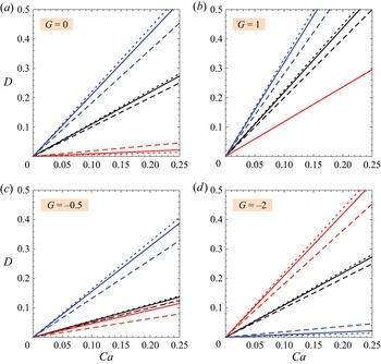
where D = 0 suggests a sphere and D → 1 denotes a slender drop. Note that we included the absolute value, as we already saw that sometimes the major radius is at ϕ = 45° and sometimes at ϕ = −45°. Figure 14 describes the Taylor deformation parameter as a function of the capillary number (Ca), the viscosity ratio (λ), the linear velocity ratio (G) and the nonlinear intensity of the flow (E). The first case (G = 0), confirms once again our finding of figure 11 (G = 0) that, for the same Ca, when E > 0, the drop is more elongated than the linear case (E = 0), and when E < 0 the drop is less elongated than the linear case. Furthermore, when E ≥ 0, as λ increases the drop is more elongated; however, when E < 0 the opposite is expected. The next case (G = 1), see also figure 12, repeats the G = 0 trends, but with a larger deformation. Here, the λ influence is practically indistinguishable for E = −1. The last two cases correspond to G < 0, where the example of figure 13 (G = −1) was not selected as it predicts no deformation for the linear case, and equal deformation (but not orientation) at E = ±1. When G = −0.5, once again, if E > 0, the drop is more elongated than the linear case and if E < 0 the drop is less elongated than the linear case. Also, as λ increases the drop is more elongated for all E cases. In the last situation, where G = −2, the major radius in all E cases is oriented at ϕ = −45°, and the deformation of the drop increases as E decreases. Moreover, when E ≤ 0 the elongation increases as λ increases, and the opposite occurs at E > 0. To summarize, the Taylor deformation parameter is primarily affected by G and E, while λ variations are of second importance.

Figure 14.

The Taylor deformation parameter, as a function of Ca, for different values of λ, G and E. Black, E = 0; blue, E = 1; red, E = −1. Solid lines, λ = 1; dashed lines, λ = 0; dotted lines, λ = 2.

6. Deformation of a very viscous drop

Taylor (Reference Taylor1934) also treated the case of a very viscous drop $(\lambda \gg 1)$, where the shape of the drop remains almost spherical, even at Ca = O(1). This is possible when the external flow has sufficient vorticity (such as in simple shear flow) resulting in the high viscosity drop rotating almost as if it were a solid particle (Frankel & Acrivos Reference Frankel and Acrivos1970; Stone Reference Stone1994). Accordingly, we repeat Taylor's solution procedure, as follows. The normal stress balance, (2.28), with the right-hand side equal to 2/Ca, is included, the normal velocities are still continuous; however, they do not vanish. Once again, with the assistance of the Mathematica software, an analytical solution of O(Ca ⁰) has been obtained. For the external flow, the coefficients of the solid spherical harmonics are now

(6.1)\begin{gather}{b_{ - 3,2}} ={+} \frac{{5(1 - \lambda )(1 + G)}}{{3(3 + 2\lambda )}} + \frac{{2(1 - \lambda )E}}{{(3 + 2\lambda )}},\end{gather}

(6.2)\begin{gather}{b_{ - 5,2}} ={-} \frac{{6(1 - \lambda )E}}{{5(11 + 10\lambda )}},\end{gather}

(6.3)\begin{gather}{d_{ - 3,2}} ={+} \frac{{(1 - \lambda )(1 + G)}}{{6(3 + 2\lambda )}} + \frac{{5(18 + \lambda - 19{\lambda ^2})E}}{{21(3 + 2\lambda )(16 + 19\lambda )}},\end{gather}

(6.4)\begin{gather}{d_{ - 5,2}} ={-} \frac{{(1 - \lambda )E}}{{15(11 + 10\lambda )}},\end{gather}

(6.5)\begin{gather}{e_{ - 4,2}} ={+} \frac{{(1 - \lambda )E}}{{30(5 + 2\lambda )}}.\end{gather}

And for the internal flow we have

(6.6)\begin{gather}{b_{2,2}} ={+} \frac{{35\lambda E}}{{(16 + 19\lambda )}},\end{gather}

(6.7)\begin{gather}{d_{2,2}} ={+} \frac{{5(1 + G)}}{{12(3 + 2\lambda )}} - \frac{{5(1 - \lambda )E}}{{2(3 + 2\lambda )(16 + 19\lambda )}},\end{gather}

(6.8)\begin{gather}{d_{4,2}} ={-} \frac{E}{{20(11 + 10\lambda )}},\end{gather}

(6.9)\begin{gather}{e_{1,0}} ={-} \frac{{(1 - G)}}{2},\end{gather}

(6.10)\begin{gather}{e_{3,2}} ={+} \frac{{7E}}{{60(5 + 2\lambda )}}.\end{gather}

Here, the other coefficients vanish, and the e_ij values are equal to the those of the previous procedure.

Following Taylor (Reference Taylor1934), we represent the surface of the drop and the surface radial velocity at the z = 0 (θ = π/2, η = 0) plane as

(6.11)\begin{equation}R(\phi ) = 1 + f(\phi ),\end{equation}

so that

(6.12)\begin{equation}{v_r} = \frac{{\textrm{d}R}}{{\textrm{d}t}} = \frac{{\textrm{d}f}}{{\textrm{d}t}} = \frac{{\textrm{d}f}}{{\textrm{d}\phi }}\frac{{\textrm{d}\phi }}{{\textrm{d}t}}.\end{equation}

While, on the other hand,

(6.13)\begin{equation}{v_\phi } = r\sin \theta \frac{{\textrm{d}\phi }}{{\textrm{d}t}} = \frac{{\textrm{d}\phi }}{{\textrm{d}t}},\end{equation}

where the last equality in (6.13) has been evaluated at the surface of the drop (r = 1) and at the z = 0 plane. Combining the last two equation results in

(6.14)\begin{equation}f(\phi ) = \int {\frac{{{v_r}}}{{{v_\phi }}}\,\textrm{d}\phi }.\end{equation}

Applying a Taylor series on v_r and v_ϕ at r = 1 and θ = π/2 for λ, around λ = ∞, suggests the following leading-order velocity components:

(6.15)\begin{gather}{v_r} = \frac{{5(1 + G)}}{{4\lambda }}\textrm{sin(}2\phi \textrm{)} + \frac{{507E}}{{380\lambda }}\textrm{sin(}2\phi \textrm{),}\end{gather}

(6.16)\begin{gather}{v_\phi } ={-} \frac{{(1 - G)}}{2}.\end{gather}

Substituting the above velocities into (6.14) and then into (6.11) results in an expression for the surface of the drop at the z = 0 plane, which at first approximation can be described as

(6.17)\begin{equation}R = 1 + \frac{{5(1 + G)}}{{4\lambda (1 - G)}}\textrm{cos(}2\phi \textrm{)} + \frac{{507E}}{{380\lambda (1 - G)}}\textrm{cos(}2\phi \textrm{)}\textrm{.}\end{equation}

With an appropriate Taylor deformation parameter of

(6.18)\begin{equation}D = \frac{{L - B}}{{L + B}} = \left|{\frac{5}{{4\lambda }}\frac{{(1 + G)}}{{(1 - G)}} + \frac{{507}}{{380\lambda }}\frac{E}{{(1 - G)}}} \right|.\end{equation}

For the familiar simple (linear) shear flow (G = 0, E = 0) in the x-direction, (6.17) and (6.18) reduce to Taylor's results. Clearly, that the treatment presented here, which we suppose to describe small deformations $(f \ll 1)$, must be restricted to $\lambda \gg 1$, Ca = O(1), G = O(1) and E = O(1), is independent of Ca and it is not valid for G → 1. When $\lambda \gg 1$ and G → 1, (6.16), as well as the previous treatment, predict, at a leading order, v_ϕ = 0, and we may expect the drop to remain at the principal axis of elongation or contraction at ϕ = ±45°.

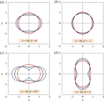
Figure 15 describes the shape of a viscous drop $(\lambda \gg 1)$, at the z = 0 plane, for different values of the linear velocity ratio (G), and of the nonlinear intensity of the flow (E). In the first case (G = 0), the deformation of the drop appears to increase with E. The largest radius is sometimes aligned with the x axis (E = 0, 1) and sometimes with the y axis (E = −1). The next case (G = −1) is interesting. Here, the drop in the linear case (E = 0) remains spherical, while the nonlinear cases deform at exactly the same magnitude but at opposite directions. Although difficult to see, for E = 1 the largest radius is aligned with the x axis and for E = −1 with the y axis. As explained above, under this very viscous drop procedure, the case G = 1 is singular, so the last two cases are dedicated to other positive values (G = 0.5, G = 2). Both cases show a relatively large deformation which increases with E. The difference is in the orientation of the drop. For G = 0.5 it is with the x axis, while for G = 2 it is with the y axis. Finally, notice that at ϕ = ±45° and ±135°, for all cases, the distance of the surface of the drop to the origin is R = 1.

Figure 15.

The shape of a very viscous drop with λ = 10 as a function of G. Black: E = 0; blue: E = 1; red E = −1.