Boron carbide complexity

Modeling B–C with classical MD is challenging due to the complex crystal structures and varying stoichiometry of its many known polymorphs. The nominal crystal structure, shown in Fig. 1(a), is described as rhombohedral consisting of primarily boron-rich icosahedra located at the unit cell vertex with a three-atom backbone chain along the [1 1 1] direction. Atomic location within these icosahedra can be subdivided into equatorial and polar sites which are shown in Fig. 1(a)’s inset as gold and gray atoms, respectively. Carbon atoms are primarily located in the backbone chain but can be substituted into distinct polar and equatorial sites of the icosahedra. Boron carbide is classified in the R$\bar 3$ m space group. However, relaxation of the atom positions and lattice parameters occur during QM and molecular statics (MS) energy minimization that disrupts this symmetry. For example, Fig. 1(b) shows a typical energy minimization routine used in this work that cycles between stages of lattice relaxation to better reduce internal pressure and relax atomic coordinate. It should be noted that common practice consists of simpler energy minimization schemes, which would follow the blue dotted-curve. Clearly, it is possible that not allowing both relaxation procedures could lead to unoptimized atomic configurations.

Figure 1.

Boron carbide is a structurally complex polymorphic material. Its lightweight and toughness make it a great candidate for a wide variety of applications. (a) visualization of a B–C rhombohedral unit cell with 12-atom icosahedra at the vertices and 3-atom chain at the body, (b) energy minimization through different molecular statics stages, and (c) atomic configuration of four B–C polymorphs known to have the lowest energy (note B₁₂CBC is boron-rich compared with the others).

Boron carbide has been experimentally observed in ranges of carbon solubility from 8 to 20 at.% without phase separation or interstitial carbon occupancy.^[Reference Thevenot^9, Reference Gosset and Colin^22] Its most abundant configurations have transition energies in the order of a few meV per unit cell (u.c.).^[Reference Domnich, Reynaud, Haber and Chhowalla^7, Reference Fanchini, McCauley and Chhowalla^23, Reference Taylor, McCauley and Wright^24] Figure 1(c) shows three 20 at.% C (B₄C) and one 13 at.% C polymorphs of boron carbide, from left to right. The two left B₄C structures in Fig. 1(c) have a boron atom inserted in the middle of the carbon backbone chain and a carbon atom substituted in the icosahedra at polar (B₁₁C^pCBC) and equatorial (B₁₁C^eCBC) sites, respectively. The right two boron carbide structures, B₁₂CCC and B₁₂CBC, have full boron icosohedra with CCC and CBC chains, respectively. Due to the atomic size difference between B and C atoms, these seemingly small variations in the polymorphic configuration lead to non-negligible structural differences.

The complexities of the boron carbide crystal structures and the thermodynamic landscape of its many polymorphs have led to difficulties in developing and parameterizing accurate interatomic potentials. Without accurate boron carbide potentials, there are no sufficient MD studies to understand the root cause of fracture nor is there clear understanding how its performance is altered due to defects.^[Reference Coleman, Hernandez-Rivera, Behler, Synowczynski-Dunn and Tschopp^5] While there has been success in observing amorphization in bulk boron carbide under shear,^[Reference An and Goddard^17] this parameterization has difficulties capturing polymorphic ordering, and predicting boron carbide defect and grain boundary structures.

Framework for parameterizing interatomic potentials

Different parameterization approaches are routinely employed in the development of interatomic potentials. Nonetheless, systematic and transferable methodologies for potential parameterization are limited. When existing potentials need to be improved upon, parameter is modified based on assumptions of potential behavior. Due to its simplicity, a common practice consists of varying parameters in a one-factor-at-a-time (OFAT) fashion. The main limitation to OFAT is that there could be hidden effects (e.g., factor interactions) which it fails to capture. Factor interactions are of interest in hyperdimensional (ℍ^D) force fields where a number of factors could influence the property of interest. Herein, a systematic statistics-based approach is proposed to parameterize and optimize these potentials.

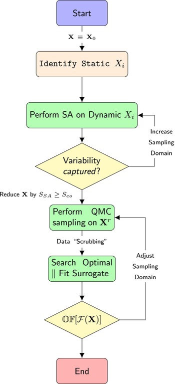
Figure 2 outlines the proposed systematic approach for parameterizing and optimizing interatomic potentials. The approach begins by adopting an initial-guess parameterization $\lpar {{\bf X}_0} \rpar $. For instance, this could be a previous parameterization which needs to be improved upon to enhance its fidelity. Herein, the potential developed by An and Goddard^[Reference An and Goddard^17] was chosen. Optimization of a large number of factors within the ReaxFF formulation can become cumbersome and expensive due to its hyperdimensionality. Therefore, the first step is to perform a SA to determine which parameters best capture response uncertainty. It is important to note that the goal is to identify a subset of factors which are exhibit importance (sensitivity) with respect to the responses of interest. Hence, parameter-space transformation approaches to dimensionality reduction, such as principle component analysis (which seek to project the data onto a reduced-order linearly uncorrelated factor space) are not directly applicable here. Identification of the most sensible parameters enables a reduction in the domain ${\open {\rm H}}^D \to {\open {\rm H}}^{d_r}$, where D ≫ d _r. The dimensional reduction is achieved by comparing sensitivity metrics. This step should be repeated until a desirable level of variability is captured. Then, a traditional design of experiments (e.g., Latin Hypercube sampling) is performed on ${\open {\rm H}}^{d_r}$ yielding statistically representative data describing how this reduced domain can predict responses (desired material properties). The sampled reduced domain is then used to determine an optimal parameterization. For instance, the sampled set could be tested against several properties of interest to determine their accuracy. Alternatively, surrogate models can be fit to the sampled data set and optimized to determine an optimal parameterization from this reduced-order models. The latter could be performed at orders of magnitude lower computational expense required of computing MS for sampled candidate usually needed of methods typically used to optimize potentials.

Figure 2.

Framework workflow for parameterizing multidimensional interatomic potentials. The framework employs several statistical techniques, resulting in optimized potential(s) that predict properties calculated from molecular statics.

Global SA enabled parameter screening

SA is a practice that helps understand how changes in independent input variables influence a model response. Understanding these relationships is paramount to being able to efficiently parameterize high fidelity interatomic potentials, especially for complex atomic systems like B–C. The ReaxFF potential permits parameterization of over 200 factors to accurately model B–C potentials, which lends itself to SA studies. However, not all these factors can be tunable as many correspond to material-specific properties (e.g. atomic mass).

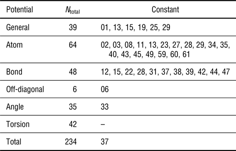
ReaxFF clearly presents dimensional challenges, and a complex computational and mathematical implementation, as evident from Eq. 1. Three prior B–C ReaxFF potentials^[Reference An and Goddard^17, Reference Paupitz, Junkermeier, van Duin and Branicio^25] were used to identify ReaxFF factors should be held constant in the current study, deeming these “material specific” or insensitive factors. Table I summarizes the findings from this comparative analysis. The integers correspond to a parameter from the given functional subset and follow the potential template nomenclature in the Supplementary Information. For example, subset atom factor 03$ \to $ ATO03 corresponds to the C atomic mass. This approach suggests that 37 of the 234 fitting factors should remain constant, resulting in a ℍ¹⁹⁷ hyperdimensional domain. In other words, we need to determine a set of 197 parameters that yield an optimal ReaxFF parameterization to describe atomic interactions between B and C atoms.

Table I.

Subset of parameters held constant from a comparative study of three prior B–C ReaxFF parameterizations from the literature^[Reference An and Goddard^17, Reference Paupitz, Junkermeier, van Duin and Branicio^25]

Optimizing the resulting ℍ¹⁹⁷ still remains computationally expensive and challenging for tractable materials design. Therefore, SA is essential for determining which of these parameters should be targeted in parameterizing the potential. Multiple techniques have been developed to perform SA on different types of mathematical systems. These include OFAT, local methods, variance-based methods, etc.^[Reference Saltelli, Ratto, Andres, Campolongo, Cariboni, Gatelli, Saisana and Tarantola^26] However, the simplicity of some techniques like OFAT can miss interactions between factors.

This work focuses on the use of the derivative-based global sensitivity measure (DGSM), which systematically changes factors yielding a measure of the global sensitivity.^[Reference Saltelli, Ratto, Andres, Campolongo, Cariboni, Gatelli, Saisana and Tarantola^26, Reference Sobol and Kucherenko^27] The DGSM is a derivative-based global method which consists of averaging the squared partial-derivative of each independent variable using quasi-random sampling techniques,

(2)$$S_{{\rm DGSM}}^{i,m} = \mathop \int \limits_{{\opf {\rm H}}^{197}} \left( {\displaystyle{{\partial f_m\lpar {\bf X} \rpar } \over {\partial x_i}}} \right)^2d{\bf X}$$

where ${\bf X} = \lcub {x_1, \ldots, x_i, \ldots, x_{197}} \rcub $ is the distribution of randomly sample factors, x _i is the independent input variable (factor) and $f_m\lpar {\bf X} \rpar $ is the MS response of interest (e.g., for B₁₂CCC 's cohesive energy $m = U_{{\rm coh}}^{B_{12}{\rm CCC}} $) obtained from MS minimization at each sampled potential. This approach has several commonalities to other better-known SA approaches like Morris screening and the Sobol sensitivity index but is able to overcome some of their limitations.^[Reference Kucherenko and Iooss^28] In fact, it is been shown that for uniformly and normally distributed input variables, the DGSM and Sobol's total sensitivity index (S _tot) are linked.^[Reference Sobol and Kucherenko^27] Further discussion on SA generalities and how it was implemented here can be found in the Supplementary Information.

The DGSMs were calculated by using the Sensitivity Analysis Library in Python (SALib) implementation.^[Reference Herman and Usher^29] SALib's finite difference sampler was used to probe ℍ¹⁹⁷, which performs a finite difference with a predefined delta (δ) around a base Sobol sequence design. This sequence is determined by assigning upper and lower sampling bounds, which defines the hyperdimensional sampling volume. These bounds were chosen by defining a bounding sampling delta (Δ) around the initial-guess potential

$$\lcub {\lpar {1 - {\rm \Delta}} \rpar \cdot {\bf X}_0 \le {\bf X}_S \le \lpar {1 + {\rm \Delta}} \rpar \cdot {\bf X}_0} \rcub $$

where ${\bf X}_S$ is the Sobol sequence and ${\bf X}_0$ is the origin potential developed by Qi.^[Reference Tschopp, Solanki, Baskes, Gao, Sun and Horstemeyer^21] The conventional finite difference sampling requires that multiples of D + 1 samples be evaluated. Therefore, a design of N _T = n · (D + 1) = 1980 samples was generated with a δ = 0.015 and a variable Δ. The former delta influences the sampling distance from each Sobol sample, while the latter controls the domain volume to be sampled. It should be noted that derivative-based measures have been found to accurately identify influential input variables from small (n ≤ 10) sample sizes.^[Reference Becker, Tarantola and Deman^30] Through MS energy minimizations on the sampled potentials, SA is performed on the objective response space ($ {\opf {\rm O}}$_DGSM). The objective response space is composed of a set of “inexpensive” material properties

$$ {\opf {\rm O}}_{{\rm DGSM}}^p = \lcub {U_{{\rm coh}}^p, V^p,a^p,\alpha^p} \rcub $$

where p is a specific polymorph, $U_{{\rm coh}}^p $ is the cohesive energy per unit cell, V ^p is the unit cell volume, a ^p is a lattice parameter and α ^p is a lattice angle.

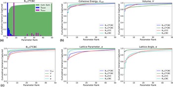
Limited to the 50 factors with the highest DGSM, the SA results are shown in Fig. 3, where the factors have been rank-ordered by their normalized DGSM. An example of B₁₁C^pCBC's cohesive energy $(U_{{\rm coh}}^{B_{11}C^p{\rm CBC}} )$ is shown in Fig. 3(a). SALib calculates a DGSM (blue bars) and a Sobol index (magenta bars) for each parameter as it relates to a specific response. The cumulative sum of the normalized DGSM (green) is representative of the variance captured. It is shown that these metrics do not agree in identifying which factor presents the highest impact on the energy response $\lpar {\hbox{max}\lpar {S_{{\rm Sobol}}^f} \rpar = S_{{\rm DGSM}}^7 \ne \hbox{max}\lpar {S_{{\rm DGSM}}^f} \rpar } \rpar $. Although the asymptotic saturation of the cumulative index supports our reasoning behind pursuing this approach (for dimensional reduction), interestingly it does not provide a clear directive on exactly how many parameters should be considered. This manifest itself with a relatively long tail to the rank-ordered DGSM. Therefore, a set of rules must be employed in determining which factors are of relevance. After rank ordering, the cumulative sum of the DGSM was plotted. Then, a threshold of 90% of the cumulative sum was chosen as the cutoff criteria. This cutoff should contain enough information to explain 90% of the variability in the sampled data. This approach was performed across ${\open {\rm O}}_{{\rm DGSM}}^p $ and polymorphs, as shown in Fig. 3(b). 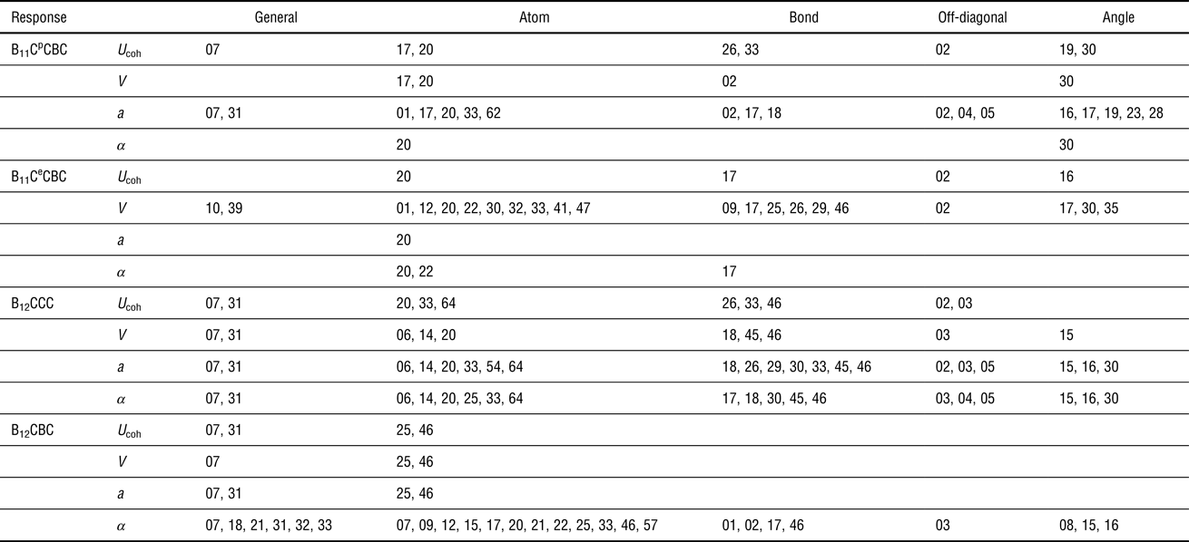From the U _coh analysis, it is observed that about seven parameters are needed to explain 90% of the observed variability in $U_{{\rm coh}}^{B_{11}C^p{\rm CBC}} $, while about three parameters are needed for $U_{{\rm coh}}^{B_{12}{\rm CBC}} $. The number and type of factor that best explain the variability also changes as a function of response within a single polymorph, as shown in Fig. 3(c). Hence, to be able to properly describe variability for such a complicated system like B–C, a set of factors is taken from the union of all these subsets. The set of factors identified as of importance are listed in Table II, which are then defined as the reduced domain $({\open {\rm H}}^{d_r} \to d_r = 55)$. It should be noted that torsion factors are excluded from the table since none were classified as important.

Figure 3.

Rank ordered DGSM values show how a limited number of factors explain most of the variance. (a) Rank-ordered top 60 parameters based on the normalized DGSM (S _DGSM), its cumulative sum and normalized Sobol index (S _Sobol), (b) cumulative variability-measure for responses and polymorphs of interest, and (c) cumulative variability-measure for the different responses of B₁₁C^pCBC.

Table II.

Parameters identified as most sensitive by the DGSM analysis

Objective and reduced domain sampling selection

The DGSM provides a measure of how much a factor is able to explain a response's variability, which allows the reduction of very large domains. Each parameter $S_{{\rm DGSM}}^{i,m} $ was then used to enable screening a factor's ability to explain variability in objective response Y _m. Further, a good parameterization requires a potential to predict multiple responses, meaning parameterizing these potentials is a multi-objective optimization exercise. Here, the focus is on inexpensive properties as defined by the response set $ {\opf {\rm O}}$_DGSM. Furthermore, the analysis focuses on the four lowest energy polymorphs, considering that these are the most abundant.^[Reference Kucherenko and Iooss^28]

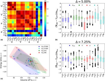
However, it is important to understand the relationship between factors and responses, and how correlation between responses could be exploited in other ways. The Pearson correlation heatmap was plotted from the SA dataset, Fig. 4(a), which shows how responses correlate across the multiple polymorphs. It is shown that cohesive energies are clustered into a high correlation region, as are the volume and lattice parameter a. For instance, the cohesive energies for the B₁₁C^pCBC and B₁₁C^eCBC polymorphs, |ρ(U(¹¹C ^p), U(¹¹C ^e))| = 0.96, are highly linearly correlated. However, the lattice parameter for B₁₂CCC and lattice angle for B₁₂CBC, |ρ(a(¹²C _l), α(¹²B _l))| = 0.26, are not correlated. Therefore, within this sampling domain, the number of responses that must be fitted can be reduced, assuming that these correlations can be used to predictably estimate changes on Y _j based on the observed changes on Y _i. For example, instead of using an objective function that aims to predict the volume of all the polymorphs, the volume of B₁₁C^pCBC could be exclusively considered. Nonetheless, as these are fairly inexpensive properties, the set of properties analyzed (U _coh, V, a, and α for each polymorph) remained unchanged.

Figure 4.

A global sensitivity analysis provides insights into the responses of interest. (a) Pearson correlation coefficient heatmap for energy, volume lattice constant, and angle for the polymorphs of interest, (b) response box-plots for two sampling bounds, and (c) Ashby-like plots of the resulting molecular statics energy minimization for the Δ = 7.25% case. (The following nomenclature was adopted: ¹¹C_p = B₁₁C^pCBC, ¹¹C_e = B₁₁C^eCBC, ¹²C_l = B₁₂CCC, and ¹²B_l = B₁₂CBC).

Interestingly, the lattice angle for all polymorphs are mostly uncorrelated. Nonetheless, it can be seen that for B₁₂CCC its lattice angle and parameter are moderately correlated, |ρ(a(¹²C _l), α(¹²C _l)| = 0.87, unlike other polymorphs. This could be due to the “symmetry disruption” that arises by the presence of C in other polymorphs’ icosahedral or backbone sites. Further, α(¹¹C ^e) is the least correlated response as analyzed from the SA results, again likely due to the symmetry challenges and structural complexity created by adding a larger C atom into an equatorial site.

A proper exploration of the ℍ¹⁹⁷ domain requires that the Δ parameter is chosen accordingly. This Δ value must sample a domain that yields a response domain where all the responses are contained within the dataset. This means that the sampled potentials yield a response domain that contains the response target (i.e., DFT) values within it, e.g., $\min (U_{{\rm coh,}}^{{\rm MS}} ) \le U_{{\rm coh}}^{{\rm DFT}} \le \max (U_{{\rm coh}}^{{\rm MS}} )$. However, for very large Δ, more Sobol samples are needed to properly sample the larger hyperdimensional volume. To determine whether the sampled volume is accurately capturing the responses, boxplots of the normalized responses are shown in Fig. 4(b) for two Δ settings. This normalization approach is similar to the “standard score”, however, instead of regressing to the mean the data was normalized to its corresponding target

(3)$$Y_i^{\prime} = \displaystyle{{{\bi Y}^i - {\bi Y}^i\; \;} \over {\sigma _{{\bi Y}^i}}} = \displaystyle{{{\bi Y}_{{\rm MS}}^i - Y_{{\rm DFT}}} \over {\sigma _{{\bi Y}_{{\rm Ms}}^i}}} \; $$

where ${\bi Y}_{{\rm MS}}^i $ are the responses obtained from MS minimization for the i-th property, Y _DFT is the target (DFT) value,^[Reference Taylor, McCauley and Wright^24] and $\sigma _{{\bi Y}_{{\rm MS}}^i} $ is the response's standard deviation. Since the response distribution is “regressed to target”, an ideal normalized response distribution encompassing the target values would be centered at zero. Therefore, the sampled potentials should yield a response distribution where the boxplot medians (red lines at notches) are approximately zero. From the ${\rm \Delta} = 5\% $ case, it can be seen that the sampled potentials yield responses that are unlikely to accurately predict target values. Furthermore, the response distribution does not encompass all the objectives since $\max (a_{{\rm MS}}^{B_{11}C^p{\rm CBC}} ) \lt a_{{\rm DFT}}^{B_{11}C^p{\rm CBC}} $. This is illustrated in Fig. 4(b), where the upper whisker of the $a_{{\rm MS}}^{B_{11}C^p{\rm CBC}} $ distribution (first red boxplot) falls below zero. This suggests that the sampling parameters (Δ and δ) are not optimal for the objective set. While maintaining δ constant, the Δ parameter is increased to sample a larger domain on ℍ¹⁹⁷. The ${\rm \Delta} = 7.25\% $ case is shown in Fig. 4(b) where the boxplots are shown to have shifted towards the zero line. While not perfectly aligned at zero, it is an improvement on ${\rm \Delta} = 5\% $. Most importantly, the response distribution fully encompasses the objective set target. Therefore, the latter could be considered a better sampling of the hyperdimensional domain as applied to B–C, which contains more robust information.

Understanding how factor modification results in property trade-offs are essential in optimizing multi-objective potentials. Ashby-like diagrams (convex-hulls) were generated for the volume and cohesive energy of the different polymorphs, Fig. 4(c). The target DFT values are shown as stars, with colors corresponding to the respective polymorph's Ashby diagram. This analysis clearly shows how the three lowest energy polymorphs fall within the center of the diagrams intersection (ca. 110 Å ³/u.c.,− 110 eV/u.c.). Hence, the resulting dataset contains enough information to properly describe the relationship between factors and these responses. However, the target values for B₁₂CBC falls just outside of this information-rich region. While some of the sampled potentials within ${\bf X}_{{\rm DGSM}}$ were able to predict the target values $U_{{\rm coh}}^{B_{12}{\rm CBC}} $ and $V^{B_{12}{\rm CBC}}$ independently (see Fig. 4(b)), these potentials did not yield a response space that contained both simultaneously, i.e., $ {U_{{\rm coh}}(V)} \vert _{B_{12}{\rm CBC}} \notin {\open {\rm O}}_{{\rm DGSM}}$. Nonetheless, it is expected that the selected sampling domain will contain enough information for a proper analysis of the ReaxFF potential. Last, it should be noted that the finite difference nature of the sampling can be appreciated from Fig. 4(c), where the scatter plots reflect the discreteness of the sampling technique.

Reduced domain parametric exploration

With a significantly reduced domain (ℍ⁵⁵) to query, a focused search can be performed on the smaller hyperdimensional domain whose bounding volume was determined from the SA. This reduced domain was sampled using 1100 Latin Hypercube samples (LHS), which is a statistical technique that generates quasi-random samples for multidimensional independent variables. The LHS technique is often used to statistically characterize high-dimensional spaces since it can yield accurate results with a reduced number of samples, with respect to traditional Monte Carlo sampling. Since LHS produces a normalized design for each dimension with values between [0, 1], the designed samples were linearly transformed to distributions bounded by ${\bf X}_0 \pm {\rm \Delta} $

(4)$$\eqalign{{\bf X}_s & = \lpar {1 + {\rm \Delta} \cdot \lpar {1 - 2{\bf X}_{{\rm LHS}}} \rpar } \rpar \cdot {\bf X}_0 \cr & = \left\{ {\matrix{ {\lpar {1 + {\rm \Delta}} \rpar \cdot {\bf X}_0,\; \; \; \; \; {\bf X}_{{\rm LHS}} = 0} \cr {\lpar {1 - {\rm \Delta}} \rpar \cdot {\bf X}_0,\; \; \; \; \; {\bf X}_{{\rm LHS}} = 1} \cr} \; \;} \right.}$$

where Δ defines the sampling distribution and ${\bf X}_{{\rm LHS}}$ is a LHS design composed of individual experiments ($({\bf X}_{{\rm LHS}}^i )$ being uniformly distributed about 0 and 1 $\lcub {{\bf X}_{{\rm LHS}} \in {\open {\rm R}}^{55}:\!\!0 \le {\bf X}_{{\rm LHS}}^i \le 1} \rcub $. As for the SA, this sampling scheme is bounded by ${\rm \Delta} = 7.25\% $ as this volume was found to be information-rich. While the idea to sample a larger volume is appealing, it must be noted that the input variables defining ${\open {\rm H}}^{d_r}$ correspond to this particular volume. Hence, exploring a larger volume might result in a different set of reduced parameters.

While the domain considered during sampling was relatively constrained, eight sampled potentials failed to converge to a stable atomic configuration during the MS energy minimization scheme. These were unsuccessful due to instabilities in the potential parameterization. Further, nine potentials converged to unphysical regimes (e.g., cohesive energies order of magnitude smaller than expected^[Reference Taylor, McCauley and Wright^24]). This unphysical regime was defined as sampled potentials resulting in values ± 10 “standard deviations” from the target (DFT) values, defined as $\sigma _{Y_i} \equiv \sqrt {Y_i} = \lpar {Y_i^{{\rm DFT}}} \rpar ^{1/2}$. Hence, a sampled parameterization ${\bf X}_i$ resulting in a cohesive energy of $\vert {U\lpar {{\bf X}_i} \rpar } \vert \gt \left\vert {U_{{\rm DFT}} \pm 10\sqrt {U_{{\rm DFT}}}} \right\vert$ would be filtered out from the 1100 sample dataset. These data were filtered to exclude potentials deemed to have resulted in poor convergence, yielding a dataset of 1083 successful potentials. The resulting “successful” dataset for B₁₁C^pCBC is graphically shown and further discussed in the Supplementary Information.

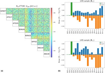
A particular challenge to hyperdimensional models is data visualization, which can enable a further understanding of the model's behavior. To address this challenge, a matrix of scatter plots for the cohesive energy of the B₁₁C^pCBC polymorph was chosen, shown in Fig. 5(a). Here, cohesive energy is represented as a function of the 8-dimensions identified in the SA as important factors (see Table II). Each box represents a 2-dimensional plane with the scattered markers representing the sampled factor distribution, and the coloring representing the cohesive energy value for the corresponding potential. It can be noticed that while these factors were identified as important, that does not necessarily make them ideal for predicting the objective response at hand. For instance, no clear trend is observed from the ATO17-ATO20 plane. However, the ATO17-BON33 plane shows a clear trend where lower values of BON33 result in higher energies. Moreover, the BON33-OFF02 plane illustrates that energies become larger as OFF02 increases. Further analysis of this plane shows that there are no main interactions between these two factors (see Supplementary Information).

Figure 5.

Exploratory and surrogate modeling-based techniques can be used to determine optimal parameterizations. (a) scatter plot matrix for B₁₁C^pCBC's cohesive energy across an 8-dimensional space, and (b) performance of two candidate potentials (which are compared to the ${\bf X}_0$^[Reference An and Goddard^17]).

The approach followed in exploring the reduced hyperdimensional space yields an information-rich refined potential samples. An exploratory approach is employed as a first step to determine suitable parameterizations and provide rigorous analysis. Two tentative suitable parameterizations (${\bf X}_{339}$ and ${\bf X}_{732}$) were identified from screening the successful samples. These were compared with the initial-guess potential ${\bf X}_0$, Fig. 5(b). The bar plots correspond to a property's error with respect to the target value, e.g., the volume error for the i −th sampled parameterization is

(6)$${\rm \Delta} V = \left \vert {\displaystyle{{V_{{\bf X}_i} - V} \over V}} \right \vert = \left \vert {\displaystyle{{V_{{\bf X}_i} - V_{{\rm DFT}}} \over {V_{{\rm DFT}}}}} \right \vert $$

where V ≡ V _DFT is the target value. Note that these measures the absolute error, hence, the bar direction (sign) is not indicative of over/underestimation. Since cohesive energies depend on the DFT implementation, the corresponding cohesive energy errors were calculated with respect to its ground state $U_{{\bf X}_i}^{B_{11}C^p{\rm CBC}} $

(7)$${\rm \Delta} U^{{\rm poly}} = \left \vert {\displaystyle{{U_{{\bf X}_i}^{{\rm poly}} - U_{{\bf X}_i}^{B_{11}C^p{\rm CBC}}} \over {U_{{\bf X}_i}^{B_{11}C^p{\rm CBC}}}}} \right \vert \; \; $$

where $U_{{\bf X}_i}^{{\rm poly}} $ is the polymorph's cohesive energy for the i −th sampled potential. This was done since capturing the correct polymorphic energetic order/trend is more important than matching a specific cohesive energy value. Several characteristics can be observed when comparing with the ${\bf X}_0$ parameterization. First, DFT values yield a trend in polymorphic energy order such that $U_{{\rm DFT}}^{B_{11}C^e{\rm CBC}} \lt U_{{\rm DFT}}^{B_{12}{\rm CCC}} \lt U_{{\rm DFT}}^{B_{12}{\rm CBC}} $. This order is not captured by ${\bf X}_0$, which predicts $U_{{\bf X}_0}^{B_{12}{\rm CBC}} \lt U_{{\bf X}_0}^{B_{11}C^e{\rm CBC}} $. Therefore, this suggests that these sampled potentials (${\bf X}_{339}$ and ${\bf X}_{732}$) are capturing some physics not observed on ${\bf X}_0$. While the refined sampling in this work yielded multiple parameterizations that capture this trend, none were as pronounced as the DFT case. It is worth noting that while parameterization ${\bf X}_{339}$ captured an average lower error across all the objectives, the polymorphic energy trend is very subtle. Parameterization ${\bf X}_{732}$ does have a more pronounced energy difference, but it results in higher errors for many of the responses.