


1. INTRODUCTION
Many applications lead us to consider models for systems that are subject to disasters or other forms of drastic intervention. Typically, these extreme events might occur intermittently at random. The first models were formulated and studied in the context of populations subject to catastrophes (see Kaplan, Sudbury, and Nilsen [3], Karlin and Tavaré [4], and Stirzaker [6]); for a more recent work in the same field, see Chao and Zheng [1]. We remark that the field of interest has been extended to include other applications such as inventory and reliability models (see Economou and Fakinos [2] and Switkes [7]). In these new contexts, the extreme event might be a regulatory intervention to reset some system within a range of acceptable values.
Here, we will be particularly concerned with models that reset the process to a value that is independent of its history up to the time of regulation or disaster. However, we do permit the times of regulation to depend on the dynamics of the system. There are several circumstances in which such models should be considered appropriate. For example, in the context of reliability models, one might postulate a system in which a random process X(t) provides some measure of the system's performance. At intervals that might depend on the amount of degradation in the system, it is restored to some pristine level of renovation.
In the context of population models, there are many examples of populations that are subject to catastrophic collapses. It is often reasonable to assume that the chance of such a collapse might depend on the size of the population. This could correspond to situations in which larger populations are more likely to lead to the exhaustion of food (or other) resources or to attract a disastrous influx of predators. In some cases, the extreme intervention might be a regulatory response to excessive levels of vermin or even bacteria. Clearly, a larger infestation is more likely to result in intervention, whereas a low level of nuisance might be tolerated.
In this article, we formulate a general framework to describe this class of processes. We derive expressions for the transient and stationary distributions of the system X(t) and hence their moments. We conclude by evaluating some of these explicitly for some typical models of interest.
2. THE GENERAL MODEL
All of the models that we consider have the following general structure. There is an underlying stochastic process U(t), t ≥ 0, that we will assume to be a regular nonexplosive Markov process in continuous time. The process U(t) is adapted to the sequence of sigma fields comprising the usual filtration,

, and we note that all of the processes considered here satisfy the usual conditions, being right-continuous with left limits.
At a time D1 > 0, the process is terminated (or killed) and a new process U1(t), t ≥ D1, replaces it. The random variable D1 is allowed to depend on the sample paths of U(t), with the constraint that the event {D1 > t} might depend only on {U(s);0 ≤ s ≤ t}; there is no functional dependence on any values of U(s) for s > t. We assume that the distribution of D1 is absolutely continuous, with density fD(x) and distribution function FD(x).
The new process U1(t), started at t = D1, is an independent and identically distributed (i.i.d.) copy of U(t) started at t = 0. Then U1(t) is terminated in the same way as U(t), after a further time D2, where D2 depends only on the path of U1(t), t ≥ D1. Then U1(t) is replaced by U2(t), t ≥ D1 + D2, where U2(t) is an i.i.d. copy of U(t). This procedure is continued indefinitely, and the process X(t), t ≥ 0, is defined to be the straightforward concatenation of the processes U(t),U1(t),U2(t),…, where the termination times of each segment correspond to the instants of regulation, intervention, or disaster, depending on the application. The random variable D1 is required to be

-measurable; that is, the event {D1 ≤ t} depends only on the path of X(t) up to time t. Note that X(t) itself is not necessarily a Markov process unless some constraint is placed on the construction of Di, i ≥ 1.
Now, by construction, the sequence Di, i ≥ 1, is a sequence of i.i.d. random variables. To this we can attach the usual associated renewal process M(t), where

In the processes we consider here,

and we assume this to be true henceforth. We next define the current life (or age) of the renewal process M(t) at time s to be the random variable C(s), where

It is well known that the distribution function FC(s)(v) of the current life is obtained from that of D by

where

and FD(k)(x) is the k-fold convolution of the distribution function FD(x) of D.
Furthermore, in the limit as s → ∞, the distribution of C(s) converges to the limit having density function given by

This holds provided that D is not arithmetic, and μD = ED < ∞, which is the case for the processes that we consider here.
The above-described structure is a more general version of that discussed by Economou and Fakinos [2] and Stirzaker [6]; in that case, the sequence Di, i ≥ 1, was assumed to be independent of the underlying process U(t). We will allow the regulating sequence to depend on the underlying process.
3. THE REGULATED PROCESS
Now we specify the distribution of the regulating intervals Di, i ≥ 1, between the terminations of the successive segments Ui, i ≥ 1, of X(t). We consider the simplest case first. Suppose that U(t) has not been terminated by time t; the essential idea is that the probability that the segment then terminates during (t,t + h) might depend only on t and on the value of U(t). More precisely, conditional on the path of U(s) up to time t, we define the termination rate τ at time t to be

for a suitable function δ(U(t),t). (In the context of reliability theory, τ(t) is familiar as the hazard-rate function.) When δ(U(t),t) does not depend on U(t), but only on t, then D1 is independent of U(t). When the function δ is additive, of the form

for suitable functions f (·) and g(·), then we are effectively assuming that the effects of time and the value of U(t) act independently in terminating the process. In later sections we will consider more general forms for τ(t), such as τ(t) = δ(U(t − d),t) or

However, for the moment we will until further notice consider the simplest case when τ is a function only of U(t):

In view of the above-discussed applications, we anticipate that the function δ(x) should be (in general) a nonnegative nondecreasing function of x ≥ 0. However, this restriction is not essential in what follows; we assume simply that δ(x) is integrable. Now denote the conditional density and distribution function of D given

by

and

, respectively. The limit in Eq. (3.1) exists because we assumed the distribution of D to be absolutely continuous, so letting h → 0 gives

It follows by integrating Eq. (3.2) that

For ease of reference, δ(x) will be called the penalty function; in particular, we will consider linear and quadratic penalty functions in specific examples. Of course, we could equally well have defined the conditional distribution of D given

by Eq. (3.3) and then derived the hazard rate in Eq. (3.1). Either way, we have the unconditional distribution of D to be

The expected value μD of D follows immediately as

Now consider the process X(t), defined in Section 2, at time s. By construction, it has the same distribution as U(C(s)), where C(s) is the current life at s of the renewal process M(s) of termination times. It follows that, conditional on C(s) = t, the distribution of X(s) is that of U(t) conditional on D > t.
This makes it possible to compute a number of properties of the process in principle and sometimes explicitly in cases of interest. For example, we have the following:
Proposition: Let the current life C(s) have distribution function FC(s)(y). The characteristic function of X(s), denoted by φX(s)(z), is given by

where I(D > t) is the indicator of the event that D > t.
Proof: Conditional on C(s) = t, we require

because eizU(t) is

-measurable. The final equality follows by the tower property for conditional expectation. █
Similar expressions can be written for the moments and the moment generating function, when they exist, and for the probability generating function whenever X(t) is integer-valued. For example, the expected value of X(s) is given by

We do not display the others, which are all similar natural modifications of Eq. (3.5).
By the continuity theorem, as s → ∞, φX(s)(z) converges to the characteristic function φX(z) of a random variable X if and only if X(s) converges in distribution, where the limiting distribution is that of X. We have remarked earlier that, as s → ∞, the distribution of the current life C(s) converges to a distribution having the density

Therefore, in this case, the limit φX(z) is given by

As earlier, similar expressions hold for the stationary moments of X(t) in equilibrium, when they exist.
In the special case when X(t) is an irreducible Markov process, then we know that its distribution converges to the stationary distribution, because it is recurrent and nonnull.
4. EXAMPLES
We consider a number of illustrative examples in detail, beginning with the simplest.
4.1. Poisson Process with Linear Penalties
Let the underlying process U(t) be a compound Poisson process; that is, the population increases at the instants of a Poisson process of rate λ and the jumps are i.i.d., integer-valued random variables Li, i ≥ 1, where each has finite moment generating function

We assume that the penalty function is linear:

This model seems appropriate when the population of interest increases mainly by sporadic immigration, possibly in groups. It also seems very appropriate for modeling the regulation of a system that deteriorates at random or an inventory with random demand for randomly sized batches of stock.
Note that in the penalty function given in Eq. (4.2), the constant term δ represents the effect of a Poisson process of rate δ that terminates the current segment independently of the size-dependent penalty θx.
Now we recall that conditional on N(t) = n, the n independent increments L1,…, Ln, of the process U(t), occur at times t − Vi, 1 ≤ i ≤ n, where the Vi are independently and uniformly distributed on [0,t]. Hence, by a standard calculation,

The mean μD is obtained by integrating this over [0,∞).
Next, by essentially the same calculation, we find the familiar result that

This, together with Eq. (3.5), supplies an expression for the moment generating function (or characteristic function) of X(s).
It is interesting to consider a special case of this process in equilibrium. Suppose that Lr = 1 for all r, so that U(t) is a simple Poisson process, and let δ = 0. Then the expected time between terminations is
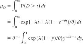
setting y = e−θt, which is finite for all λ > 0 and θ > 0.
Furthermore, from Eq. (3.6) we have the stationary probability generating function π(z) of X(t) in equilibrium:

setting y = e−θt. Hence, or directly, we find the stationary expected value of the population size in equilibrium, in the form

which is finite for all λ > 0 and θ > 0. Similar expressions can be written for any required moment.
As we have noted earlier, one can in principle obtain this by solving the usual equations for the stationary distribution of X(s), but the above approach seems to have clear advantages.
4.2. Yule Process with Linear Penalties
Let the underlying process be U(t) = Y(t), where Y(t) is the simple birth process (Yule process) with Q-matrix given by qj,j+1 = λj, and qjj = −λj, for all j ≥ 1.
This is an appropriate model when the population of interest increases mainly by reproduction. At a catastrophe, the process is returned to Y(0) = 1.
Again, we assume linear penalties, so that

It is well known that Y(t) is geometric with parameter e−λt. It is equally well known that, conditional on Y(t) = y + 1, the y events of the process (i.e., the births) occur at times t − Bi, 1 ≤ i ≤ y, where the Bi are i.i.d. on [0,t] with density

and moment generating function

A small modification of the arguments used above for the Poisson process will therefore yield any required results of interest. Let us consider only the stationary distribution of X(t) in the case when δ = 0. Omitting the details, which resemble those in Eq. (4.3), we find that

The mean μD is obtained by integrating this over [0,∞). Note that it is finite and note the special case when λ = θ, yielding

For the stationary distribution of X(s), we find likewise, and as earlier from Eq. (3.6), that

Hence, or directly, the mean in equilibrium is

Next, we consider an example when the underlying process U(t) is not monotone nondecreasing.
4.3. Reflected Wiener Process with Quadratic Penalties
Let the underlying process be U(t) = |W(t)|, where W(t) is the standard Wiener process. Of course, |W(t)| is simply the Wiener process reflected in the origin.
This process might be seen as a continuous limit of the symmetric random walk in continuous time and is therefore appropriate when the underlying system fluctuates symmetrically in this way. Switkes [7] has considered this symmetric random walk in the presence of a process of catastrophes that are independent of the walk, suggesting a number of applications.
We let the penalty function in this case be quadratic, so that

This penalty function has the advantage of being symmetrical about the origin. The symmetry of the distributions of W(t) about the origin allow us to define X(t) as |Xw(t)|, where Xw(t) is the regulated process obtained when the underlying process is the standard Wiener process W(t).
We follow the by now familiar schedule of calculations to see that as usual

by the Cameron–Martin formula. (See, for example, Revuz and Yor [5].)
The expected value of D, obtained by integrating Eq. (4.9) over [0,∞), can then be expressed as an elliptic integral.
The Markov process X(t) is irreducible and recurrent, so we can consider the stationary expected value in equilibrium, μX.
Here

is the usual filtration appropriate for the Wiener process; recalling the Eq. (3.6) we obtain an expression for μX as follows:

Now we remark that conditional on W(0) = 0 and W(t) = w, the process W2(u) is the squared Bessel bridge over [0,t].
For this process, the internal conditional expectation in Eq. (4.10) is given by the Pitman–Yor formula (see Revuz and Yor [5]) and we have

Hence, the stationary mean of the regulated process X(t) in equilibrium is, on removing the conditioning on W(t), which we know to have the N(0,t) density,

which is finite for all θ > 0.
In exactly the same way, it is straightforward to write similar expressions for any moment of X(t) in equilibrium.
5. FURTHER EXAMPLES
In all of the examples discussed in Section 4, the penalty δ was a function simply of U(t) (linear or quadratic). However, as we remarked in the discussion at the beginning of Section 3, there are many practical applications in which the penalty and consequent regulation should depend on other properties of the process up to time t.
For example, it is reasonable to consider the possibility of delays in regulation. There might be lags in the collection and reporting of data about the system, or the regulatory response might be deferred, or both. In such cases, the penalty function δ might be expected to be defined in terms of U(s) for s < t.
In the simplest case, naturally, we assume that the dependence on the state at some earlier time is linear and, for some constant d > 0, write

The analysis following Eq. (3.2), leading to Eqs. (3.4)–(3.6) now follows essentially as earlier, provided that the argument t is replaced by t − d as appropriate. We consider two examples later in this section.
We will also consider some other simple and natural models for the penalty function δ; the general property that they all share is that at time t, δ is a function of U(s) for s ∈ [0,t]. In no case do we permit the penalty to have any functional dependence on values of U(s) for s > t.
5.1. Poisson Process with Delayed Penalty
We assume that the underlying process U(t) is the standard Poisson process of rate λ and that the penalty function is that given in Eq. (5.1). Let the random variable D(d) be the time of first termination. Then, trivially, for t ≤ d, we have P(D(d) > t) = 1. For t > d, the usual schedule of calculations yields

where D is the termination time defined in Section 4.1 for the Poisson process with linear penalty when d = 0. Hence, immediately, the mean is given by

where μD is as given in Section 4.1.
Now let μX(d) denote the stationary expected value in equilibrium of this regulated process X(t) with delayed penalty. By the results of Section 3, in the usual way, we have that

using the results for the case in Section 4.1. Hence,

Likewise for the stationary probability generating function πd(z) of the process X(t) in equilibrium, we have

where π(z) is the stationary probability generating function of the Poisson process with linear penalty given in Eq. (4.5). Substituting for μD(d) using Eq. (5.2) gives the required expression for πd(z).
5.2. Reflected Wiener Process with Delayed Penalty
Let the underlying process be U(t) = |W(t)|, where W(t) is the standard Wiener process. We assume that the penalty function is

With the notation following that introduced in Section 5.1, it follows in the usual way that the expected time of termination is

where μD is obtained by integrating Eq. (4.9), as usual. Now let μX(d) be the stationary expected value of the regulated process in equilibrium. In order to calculate this, we recall three results:
I. From Section 4.3 we recall the Pitman–Yor formula

where


It is easy to show that Bt < 0 for t > 0.
II. The reflected Wiener process |W(t)| = Y(t), started at Y(0) = w > 0, has density function

where φ(t,x) is the density of the normal N(0,t) random variable X. Note that fY(t,y;w) is an even function of

; a fact that we will use shortly.
III. Let the random variable Z be normally distributed with mean zero and variance t − d; that is, N(0,t − d). Then for any real y and B < 0,

This is readily verified by a routine integration, which we omit.
Now we can calculate, as usual,

The integrand in the last term in Eq. (5.12) can be written as

because fY(d,y;w) is an even function of w (as we noted in result II) and the distribution of W(t − d) is symmetric about the origin; the interchange of integration and expectation is justified using the nonnegativity of the integrand.
The expectation in the integrand in Eq. (5.13) can be evaluated using conditional expectation and the Pitman–Yor formula (see Eq. (5.7)), as

where At and Bt are given by Eq. (5.8) and Eq. (5.9), respectively. Now

so that using Eq. (5.11) in result III, we obtain

Hence, from Eqs. (5.12)–(5.15),

setting t − d = s in the integral.
By the same argument, it is straightforward to obtain similar expressions for the stationary moments of X(t) in equilibrium, if desired.
5.3. Poisson Process with Integral Penalty
Finally, we note that in several applications it is reasonable to assume that the penalty at t should not depend just on U(t), but also on the cumulative effect of its path up to time t. For an example, consider the effect of a population on the environment. Perhaps the simplest model that takes account of this case arises when the penalty function is assumed to be

Then, with the usual notation,

Now let U(t) be a Poisson process of rate λ and recall that conditional on U(t) = n, the n events of the process occur at times t − Vi, 1 ≤ i ≤ n, where the random variables Vi are independently and uniformly distributed on [0,t]. Let their order statistics be V(i), 1 ≤ i ≤ n. Then, conditional on

, we find that

after integration and rearrangement. Hence, using Eq. (5.17),

As usual, μD is obtained by integrating this over [0,∞). For the stationary moment generating function M(ψ) of X(t) in equilibrium, we use Eq. (3.6) in the usual way to give

Hence, or directly, the stationary mean μX in equilibrium is found to be given by

Similar expressions can be written for any moment in the same way. In conclusion, we note that the same methods can be used to yield equivalent results for the Yule process with an integral penalty; the uniform distribution of Vi in (5.18) is replaced by

as in Section 4.2.
Likewise, very similar calculations will deal with the Poisson and Yule processes with a product penalty function of the form

We omit the details.


