




No CrossRef data available.
THE TIME-TO-EMPTY FOR TANDEM JACKSON NETWORKS
Published online by Cambridge University Press: 01 October 2004
Abstract
We derive the distribution of the time-to-empty for an open tandem Jackson network assuming that while in equilibrium at time 0, the arrival stream is suddenly shut off. The analysis is based on analogous results regarding the distribution of the time-to-empty for the corresponding closed tandem Jackson network. The results obtained are used in the analysis of a two-class tandem Jackson network with FIFO discipline in which customers of the second class have negligible service times.
Information
- Type
- Research Article
- Information
- Probability in the Engineering and Informational Sciences , Volume 18 , Issue 4 , October 2004 , pp. 493 - 502
- Copyright
- © 2004 Cambridge University Press
1. INTRODUCTION
We consider a open tandem Jackson network with M single-server exponential stations with service rates μm, m = 1,2,…,M, and external Poisson arrivals with rate λ < minm=1,…,M μm. Assuming the process to be in equilibrium, we are interested in the distribution of the time it takes for the system to empty if at time t = 0 the arrival process is suddenly switched off.
More formally, consider the continuous-time Markov chain

with state space

and generator

(Here, em = (0,0,…,1,…,0) is the unit vector in the mth direction in

and (0,0,…,0) acts as an absorbing state.) The above process, together with the initial condition

, describes the behavior of the open tandem Jackson network when the arrival process is switched off at time t = 0.
Note that the time-to-empty is precisely the flow time through the network of a virtual customer who arrives at time t = 0 and finds the system in equilibrium and whose service time is zero at all stations. Thus, the time-to-empty can be thought of as a generalization of the workload (or virtual waiting time) for a tandem network. In Section 4, we take advantage of this remark to apply the results obtained to the analysis of a two-class FIFO tandem network in which customers of the second class have negligible service times.
Let τ = inf{t ≥ 0 : X(t) = (0,0,…,0)} be the time required for the system to empty. In order to compute the Laplace transform R(s) := Ee−sτ, we first condition on the number of customers in the network at time 0. If we denote by
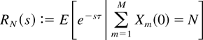
the Laplace transform of τ conditional on having N customers in the system initially, then

The total number of customers in the system in steady state for the original open Jackson network, before the arrival process is switched off, can, of course, be obtained as the sum of M independent geometric random variables and, thus, its probability generating function takes the form

where the constants

are determined by a partial fractions expansion. The above expansion is, of course, valid only if the service rates are different from each other [i.e., μm ≠ μl (and, thus, ρm ≠ ρl) for m ≠ l], an assumption which we will adopt for simplicity in the sequel. Thus, we have

In order to evaluate RN(s), it suffices to realize that this is the same as the time to emptiness for the corresponding closed Jackson network in equilibrium if, at time 0, we “break the loop” and suppose that customers who finish service at station M simply leave the system and do not return to station 1. In the next section, we will see how this can be evaluated by turning what is a question regarding the transient behavior of the network into a question regarding its steady-state operation.
2. A RECURSIVE RELATIONSHIP FOR THE TIME-TO-EMPTY IN TANDEM CLOSED NETWORKS
Consider the same tandem network as earlier which we now assume operating as a closed Jackson network with N customers. In fact, we will consider a whole family of closed network processes, each described by a continuous-time Markov chain,

with state space

defined on a probability space

, where XN(t) = (X1N(t),…,XMN(t)) denotes the number of customers in each station at time t. We assume that the Markov chain XN is stationary under P and we denote by {DnN} the point process of departures from node M. We use the standard numbering convention that D0N ≤ 0 < D1N P-a.s. (i.e., call D1N the first point strictly to the right of the time origin) and denote by

, the interdeparture times. We will also denote by PN0 the Palm transformation of the probability measure P under the point process {DnN} and by EN0 the expectation with respect to PN0.
If we were to assume that at time 0 “the loop is broken” between station M and station 1 so that customers who finish service at station M simply leave the system without returning, then, because at time 0 the system is a closed network in equilibrium, the time for the system to empty is precisely DNN, the time until the Nth departure in a closed network with N customers in equilibrium. This, of course, is true since all stations have single servers so that it is not possible for one customer to overtake another. Thus,

We are now ready to establish the following theorem.
Theorem 1: The time-to-empty starting from equilibrium for a closed tandem Jackson network with N customers is given by the expression

where λk is the throughput in such a network with k customers and R1(s) is the time to emptiness from equilibrium in the network with a single customer given by
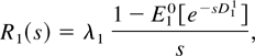
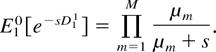
where
Proof: We will use the approach in [10] (see also [12]) as follows. Let XN+1 be the same closed Jackson network with N + 1 customers and suppose that it is stationary under P. If we denote by {DnN+1} the departure process for this system and if PN+10 denotes the Palm probability transformation of P under {DnN+1}, then, as a consequence of the arrival theorem (see [3,6,7,8,9]), we have

However, by the shift invariance properties of PN+10 and since PN+10(D0N+1 = 0) = 1, we also have
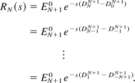
Using the above equations in conjunction with the arrival theorem, we conclude that

(In the above argument, note that RN(s) is originally expressed as a stationary expectation, then the arrival theorem is used to express it as a Palm expectation in a network with one additional customer, then a shift is performed along the points of the departure process, and, finally, the arrival theorem is used once more to return to a stationary expectation in the original network with N customers.) Using the Palm inversion formula (see [1]), we obtain the relationship
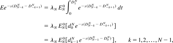
where in the last equation we have again used the shift invariance of PN0. From (8) and (9), adding term by term, we obtain
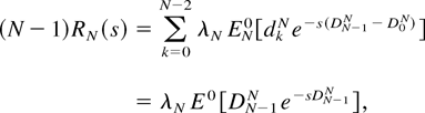
where in the above equation we have taken into account that PN0–a.s. D0N = 0 and DN−1N = d0N + d1N + ··· + dN−2N. However, we have
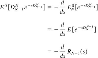
(where we have used the arrival theorem again!) and, hence, (10) can be written as

Applying the above recursively we readily obtain (5). It remains to establish (6), which, however, follows immediately by applying the Palm inversion formula once more. (This should be intuitively obvious: R1(s) = E [e−sD11] is simply the forward recurrence time of the departure process {Dn1} in the closed network with a single customer in equilibrium.) Finally, (7) clearly holds since D11 under P10 is the typical cycle time in a closed tandem network with a single customer. █
From Theorem 1, it is clear that the explicit computation of RN(s) is not difficult. In the next section, we carry out this computation and we return to the problem of the open network.
3. CLOSED-FORM EXPRESSIONS FOR THE TIME-TO-EMPTY IN CLOSED AND OPEN JACKSON NETWORKS
Here, we will assume for simplicity that the service rates in different nodes of the network are different (μm ≠ μl when μ ≠ l). Under this assumption, it has been shown in [10] that
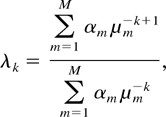
where

The constants αm arise from the partial fractions expansion
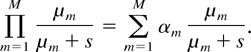
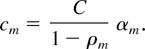
If we set

, then it is easy to see that these constants are connected to the constants (3) via the relationship
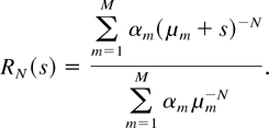
From (5)–(7), (12), and (14), after some elementary manipulations, we obtain the following closed-form expression for the time-to-empty for a closed tandem Jackson network initially in equilibrium with N customers:
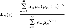
It is interesting to compare the above formula with the expression for the Laplace transform of the cycle time of a customer in this network with N customers, which we will denote by ΦN(s), as given in [10]:
We are now in a position to compute the Laplace transform of the time-to-empty for the open tandem Jackson network in steady state. From (1), (4), (15), and (16), we obtain

Again, the comparison with the corresponding flow time (viz. the time it takes from the moment a customer arrives to the first station until the time it leaves the last station in steady state) is interesting. If this flow time is denoted by Φ(s), then it is well known (e.g., see [7,9]) that
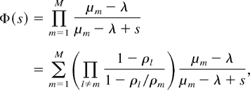
the second expression equality following by a partial fractions expansion of the first.
Finally, we compute the Laplace transform of the time-to-empty for the same system assuming that at time 0 it is in steady state and conditioning on the event that there are N or more customers in the system. Elementary manipulations similar to the ones described earlier give
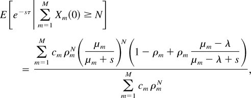
where the constants cm are given in (3). Note the similarity of the above expression with the corresponding result for the M/M/1 queue. Suppose that an M/M/1 system with arrival rate λ and service rate μ > λ is in equilibrium at time t = 0 and that at that time, the arrival process is switched off. Then, the Laplace transform of the time required for the system to empty can be easily computed via a conditioning argument and is equal to

where ρ = λ/μ. It is worth noting that the corresponding result for the tandem network given in (20) is simply a weighted average of the corresponding M/M/1 factors for each station.
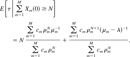
From (20), we can readily obtain the mean time for the network to empty given that there are at least N customers in the system:
4. APPLICATION: A TWO-CLASS TANDEM NETWORK WITH PROBE CUSTOMERS
Consider now an open, tandem Jackson network with two classes of customers. Customers belonging to the first class arrive to the system according to a Poisson process with rate λ and their service rates at the M stations are μ1,μ2,…,μM, as earlier. Customers belonging to the second class arrive according to an independent Poisson process with rate ν and the service discipline is FIFO for all customers and stations. We will assume that the service times of class 2 customers at the various stations are so small compared with the timescale of the system that we can entirely ignore them. Thus, these customers, which we will call probe customers, flow through the system without delay except for the fact that they have to wait in front of class 1 customers. There are many cases in both communications systems and in manufacturing where such a model is applicable. Then, one can easily see that the flow time of the typical probe customer is precisely the time-to-empty for the Jackson network in equilibrium with only one class of customers. Thus, (18) gives the flow time for probe customers also. Let us now denote by Π(z) the probability generating function (p.g.f.) of the stationary number of probe customers in the system. Then, we can use the distributional law of Little (see [4,5]) to obtain

Thus, the stationary distribution of probe customers is expressed as a combination of geometric factors.
One might be tempted to derive Π(z) directly by noting that the number of probe customers who arrive between two consecutive class 1 customers is geometrically distributed with p.g.f. given by λ/(λ + ν − νz) and then composing this p.g.f. with the p.g.f. of the total number of class 1 customers in the system, as given in (2). Such reasoning, however, will not lead to the correct result since the number of class 1 customers in the system at any given time and the interarrival intervals corresponding to these customers are, of course, not independent.
Clearly, as long as the process of class 1 customers is in steady state, the flow time of probe customers will be given by (18), regardless of the statistics of their arrival process, provided, of course, that this arrival process is independent of the arrivals and service requirements of class 1 customers. What could become more complicated is the determination of the statistics of the total number of probe customers in the network. However, when probe customers arrive according to a renewal process with interarrival distribution G, independent of the arrivals and service times of class 1 customers, then, as we will see, the stationary number of probe customers in the system can be easily determined. This is done using the distributional version of Little's law for renewal arrivals in the form given in [11] (see also [2]).
In the framework adopted there, one starts with a marked point process

, which is assumed to be stationary under the probability measure P. The marks Wn are assumed to be nonnegative w.p. 1. Corresponding to this marked point process, one defines the arrival counting measure

, where B is any Borel set in

, and the system size process

. Tn is to be interpreted as the arrival epoch of the nth customer, Wn as his sojourn time through the system, and Y(t) as the total number of customers in the system at time t. In our situation, {Tn} is the renewal arrival process of probe customers, {Wn} is their corresponding sojourn times through the network, and Y(t) is the total number of probe customers in the network at time t. We will also denote by P* the Palm transformation of P with respect to the point process {Tn}. Let Π(z) := EzY(0) denote the p.g.f. of the stationary number of probe customers in the system. In [11], it is shown that

where

is the mean interarrival time, assumed finite, provided that the following two conditions hold:
1. The system is FIFO (i.e., Tm + Wm ≤ Tn + Wn w.p.1 whenever m < n).
2. The system enjoys the following Lack of Anticipation Property: Under P*, W0 and A(0,u] are independent for all u > 0. This simply states that the sojourn time of a customer cannot be influenced by future arrivals, and future arrivals, in turn, do not contain any information regarding the sojourn time of the customer who arrives at time 0.
In our situation it is clear that both conditions are satisfied. Also,

, and if we denote by

the Laplace transform of G, a straightforward computation gives

where we have used the notation

to denote the Laplace transform of the integrated tail distribution that corresponds to G. In view of (18) and (3), we have

Thus, from (22)–(24), we conclude that

The above displays the total number of probe customers in the system as a combination of geometric factors.
References
REFERENCES
Bertsimas, D. &
Nakazato, D.
(1995).
The distributional Little's Law and its applications.
Operations Research
43:
298–310.Google Scholar
Brémaud, P.,
Kanurpatti, R., &
Mazumdar, R.
(1992).
Event and time averages: A review.
Advances in Applied Probability
24:
377–411.Google Scholar
Haji, R. &
Newell, G.F.
(1971).
A relation between stationary queue and waiting–time
distributions.
Journal of Applied Probability
8:
617–620.Google Scholar
Keilson, J. &
Servi, L.D.
(1988).
A distributional form of Little's law.
Operations Research Letters
7:
223–227.Google Scholar
Lavenerg, S.S. &
Reiser, M.
(1980).
Stationary state probabilities at arrival instants for closed
queueing networks with multiple types of customers.
Journal of Applied Probability
17:
1048–1061.Google Scholar
Sevcik, K.C. &
Mitrani, I.
(1981).
The distribution of queueing network states at input and output
instants.
Journal of the Association for Computing Machines
28:
358–371.Google Scholar
Walrand, J.
(1988).
An introduction to queueing networks.
Englewood Cliffs, NJ:
Prentice-Hall.
Zazanis, M.A.
(1997).
Formulas and representations for cyclic Markovian networks via
Palm calculus.
Queueing Systems
26(1–2):
151–167.Google Scholar
Zazanis, M.A.
(1998).
Functional versions of Little's law.
Stochastic Processes and Their Applications
74(2):
195–201.Google Scholar
Zazanis, M.A.
(2004).
Cycle times in single server cyclic Jackson networks.
Operations Research Letters
32(5):
422–430.Google Scholar
 You have
Access