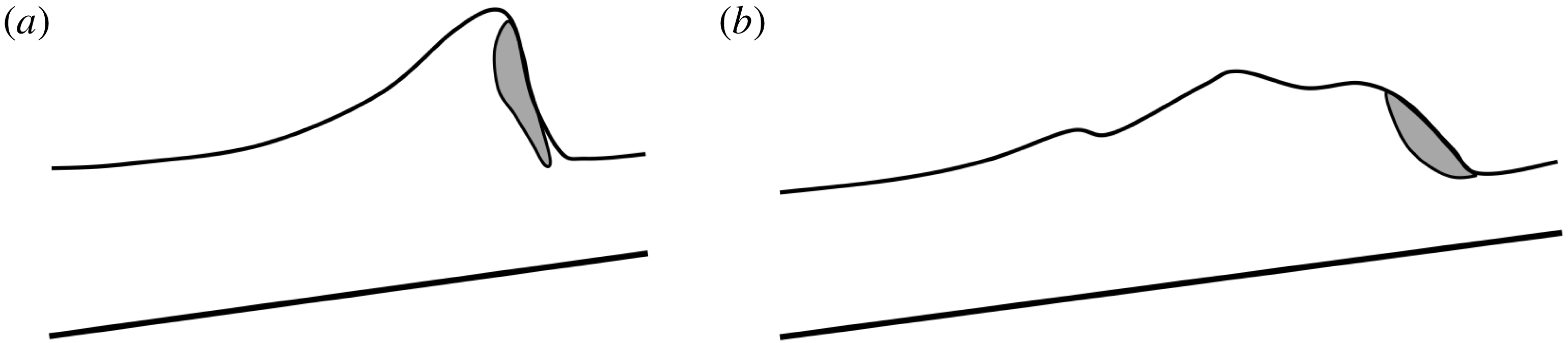
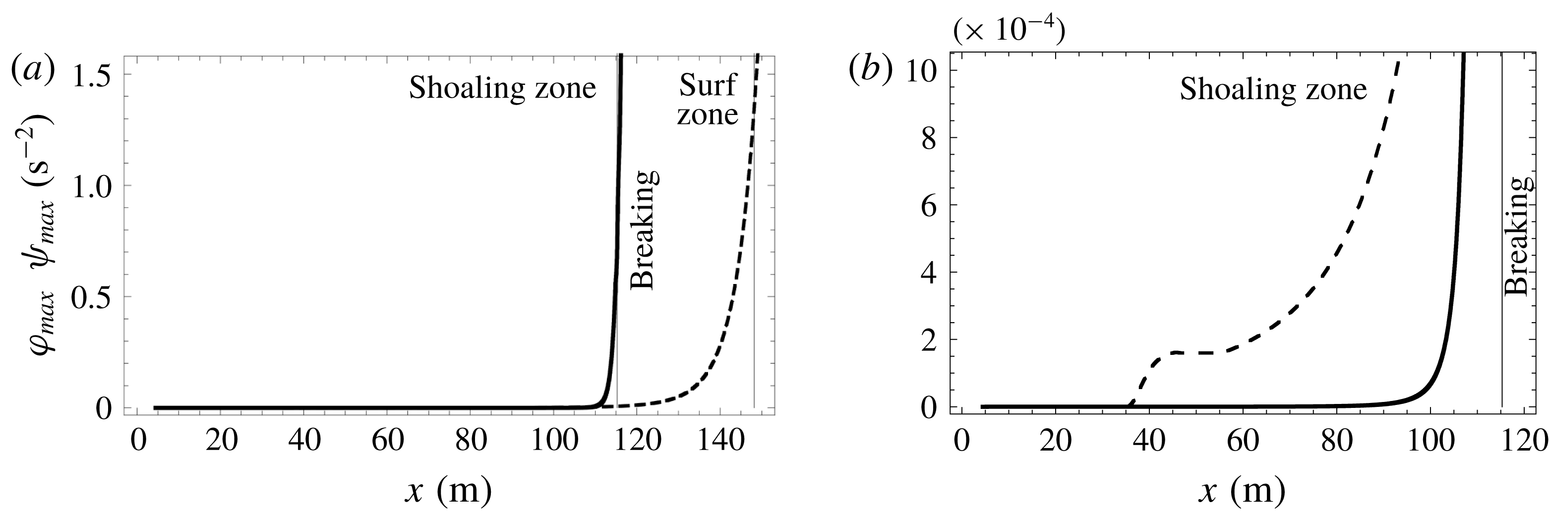
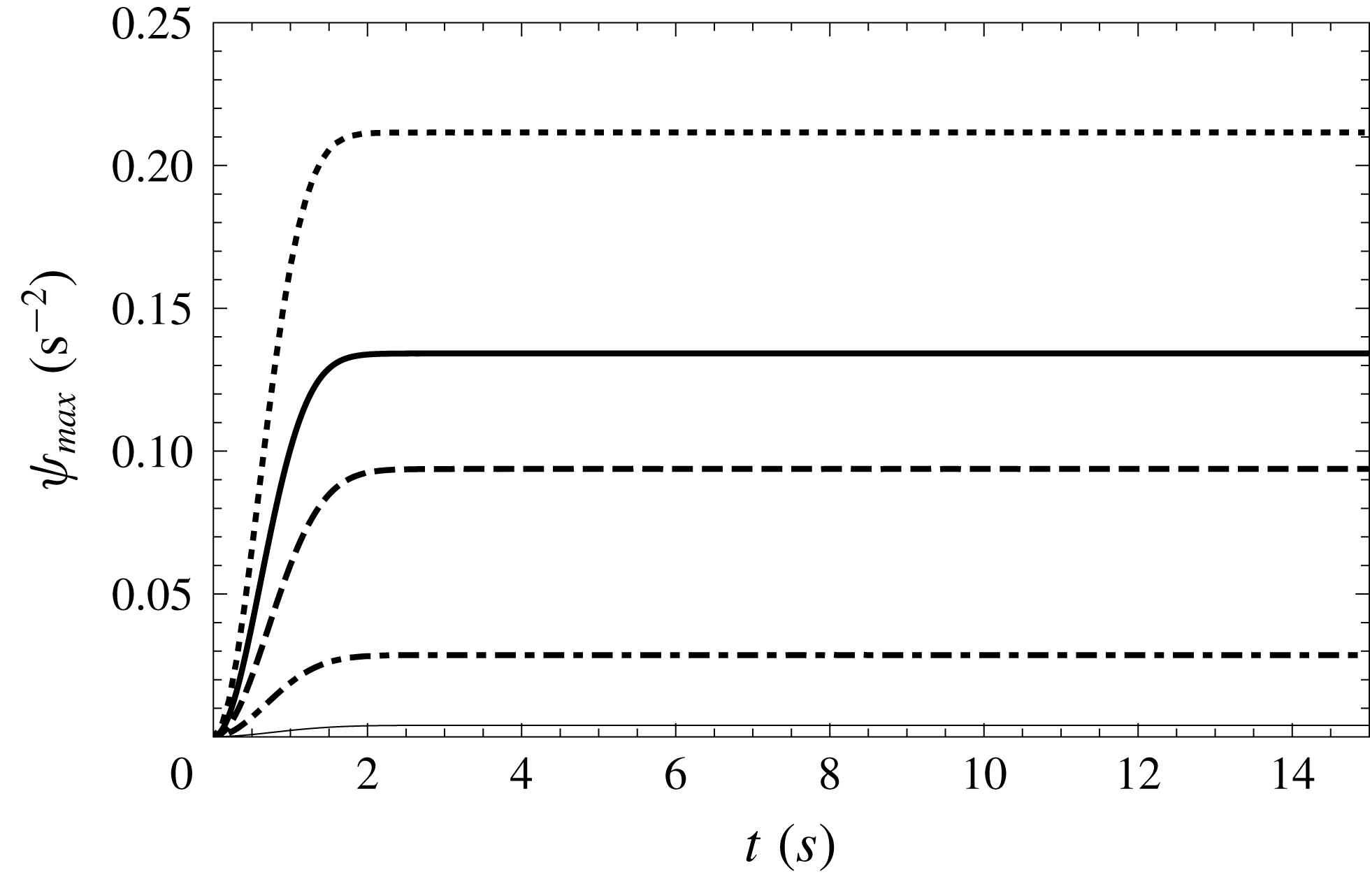
1 Introduction
Mathematical modelling of coastal wave propagation is a quite challenging issue since it is difficult to describe in the same model the dispersive effects in the shoaling zone and the energy dissipation of breakers in the surf zone. As it is impractical to solve the full Navier–Stokes system over any significant domain, approximate models must be used. Many asymptotic models were proposed in the last decades for the coastal wave propagation.
The first attempt to describe a surf zone wave propagation was made in the context of the nonlinear shallow-water equations, also called the Saint-Venant equations (Barré de Saint Venant Reference Barré de Saint Venant1871). Meyer & Taylor (Reference Meyer and Taylor1972) reviewed analytic solutions of the shallow-water equations over a beach. Stocker (Reference Stocker1957) presented perhaps the first numerical solution of the shallow-water equations for a sloping beach using the method of characteristics. His method produces quite accurate results for the simple cases. Freeman & Le Méhauté (Reference Freeman and Le Méhauté1964) and later Iwasaki & Togashi (Reference Iwasaki and Togashi1970) improved this method. However, when the characteristic lines cross at the breaking point the wave evolution has to be treated in a different manner. Further for non-uniformly sloping beaches, this method is cumbersome.
In order to be able to calculate the wave breaking, Hibbert & Peregrine (Reference Hibbert and Peregrine1979) proposed a ground-breaking method based on the numerical solution of the nonlinear shallow-water equations in their conservative form. This method gives physically realistic results. However it is not very robust in the run-up phase (Synolakis Reference Synolakis1989). Furthermore, it is important to take into account a large energy dissipation following the wave breaking. Consequently, a subsequent version of this algorithm (Packwood & Peregrine Reference Packwood and Peregrine1981; Kobayashi, Otta & Roy Reference Kobayashi, Otta and Roy1987) added artificial dissipative terms such as viscosity and friction for an accurate wave amplitude description.
Indeed the nonlinear shallow-water equations give a rather good description of breaking waves representing them as shocks, and the run-up simulations generally give accurate results. However due to the absence of dispersive effects the wave profile is not described precisely, particularly in the shoaling zone. Moreover this model predicts that all waves break, which is obviously incorrect. Thereby, a more relevant modelling of wave shoaling before breaking is based on various Boussinesq-type models (Brocchini & Dodd Reference Brocchini and Dodd2008). Non-breaking numerical solutions for the Boussinesq equations are reviewed by Liu, Synolakis & Yeh (Reference Liu, Synolakis and Yeh1991). Since the 1990s, considerable efforts were made to improve the dispersive properties of the Boussinesq model (Madsen & Sørensen Reference Madsen and Sørensen1992; Nwogu Reference Nwogu1993; Wei et al. Reference Wei, Kirby, Grilli and Subramanya1995). A review of Boussinesq-type models was performed recently by Brocchini (Reference Brocchini2013).
Most of the Boussinesq models are derived in the assumption of a weak nonlinearity (the wave amplitude is much smaller than the characteristic water depth). The natural idea is to use a fully nonlinear model, such as the one derived by Serre (Reference Serre1953) and Su & Gardner (Reference Su and Gardner1969), in the one-dimensional (1-D) case, or the two-dimensional (2-D) fully nonlinear model presented in Green & Naghdi (Reference Green and Naghdi1976). This model can be derived from the Euler equations as an asymptotic model in the shallow-water regime without any hypothesis on the wave amplitude (see e.g. Lannes Reference Lannes2013). This fully nonlinear model has better dispersive properties than the Boussinesq equations, and the water wave profile is better described. Except for being formulated in terms of the velocity vector at an arbitrary level, the equations of Wei et al. (Reference Wei, Kirby, Grilli and Subramanya1995) mentioned above are basically equivalent to the 2-D Green–Naghdi equations. In fact, the Green–Naghdi equations are often known in the literature as the fully nonlinear Boussinesq-type model. The dispersive properties of the Green–Naghdi equations were further improved by Bonneton et al. (Reference Bonneton, Chazel, Lannes, Marche and Tissier2011) and Chazel, Lannes & Marche (Reference Chazel, Lannes and Marche2011).
However the weakly nonlinear or fully nonlinear Boussinesq-type equations do not include dissipation due to wave breaking, and thus become invalid in the surf zone. To extend the validity of these equations, Heitner & Housner (Reference Heitner and Housner1970) introduced an artificial viscosity term into the momentum balance equation. This approach was followed by many researchers. Zelt (Reference Zelt1991) used an eddy viscosity formulation together with a Lagrangian Boussinesq model. The inclusion of this term in the momentum equation helps to control the energy dissipation, and it must be calibrated with experiments. Similar techniques were used in Madsen, Sørensen & Schäffer (Reference Madsen, Sørensen and Schäffer1997), Wei, Kirby & Sinha (Reference Wei, Kirby and Sinha1999) and Kennedy et al. (Reference Kennedy, Chen, Kirby and Dalrymple2000). Another idea is to use the so-called roller models which include dissipation through an extra convective term in the momentum equation (see for example Schäffer, Madsen & Deigaard Reference Schäffer, Madsen and Deigaard1993; Svendsen, Yu & Veeramony Reference Svendsen, Yu, Veeramony and Edge1996; Karambas & Tozer Reference Karambas and Tozer2003; Briganti et al. Reference Briganti, Musumeci, Bellotti, Brocchini and Foti2004; Musumeci, Svendsen & Veeramony Reference Musumeci, Svendsen and Veeramony2005; Dimas & Dimakopoulos Reference Dimas and Dimakopoulos2009; Cienfuegos, Barthelemy & Bonneton Reference Cienfuegos, Barthelemy and Bonneton2010; Viviano, Musumeci & Foti Reference Viviano, Musumeci and Foti2015). The basis of these models is the concept of surface roller due to Svendsen (Reference Svendsen1984). In this approach additional terms are included not only in the momentum equation, but also in the mass balance equation and the thickness of the roller region has to be estimated.
In the so-called switching or hybrid approach the dispersive terms are suppressed in the breaking regions. Contrary to the nonlinear shallow-water system, the Boussinesq equations do not admit discontinuities because they are dispersive. The removal of the dispersive terms reduces the system to the nonlinear shallow-water equations. This relatively simple idea was developed in many studies (for example Bonneton et al. Reference Bonneton, Chazel, Lannes, Marche and Tissier2011; Tonelli & Petti Reference Tonelli and Petti2011; Shi et al. Reference Shi, Kirby, Harris, Geiman and Grilli2012; Tissier et al. Reference Tissier, Bonneton, Marche, Chazel and Lannes2012; Kazolea, Delis & Synolakis Reference Kazolea, Delis and Synolakis2014; Duran & Marche Reference Duran and Marche2015, Reference Duran and Marche2017; Filippini, Kazolea & Ricchiuto Reference Filippini, Kazolea and Ricchiuto2016).
A complete and detailed overview of these approaches can be found in Brocchini (Reference Brocchini2013) and in Kirby (Reference Kirby2016). Generally speaking, two large groups of methods can be distinguished. The first one includes additional terms such as viscous terms and the second one uses hybrid methods. In both approaches some parameters need to be calibrated. Moreover some criteria must be defined to initiate or terminate the breaking process. Generally, these criteria are based on different empirical relations. For example, the breaking process is activated if the wave local energy dissipation forms a peak, or if the wave slope reaches a critical value.
Detailed analysis of the different approaches cited above and an estimation of the influence of the numerical dissipation can be found in Kazolea & Ricchiuto (Reference Kazolea and Ricchiuto2018). The authors highlight that, despite the absence of an explanation for the physical meaning of the coefficients in the eddy viscous terms, this approach shows little sensitivity to the grid, while hybrid methods are not very robust and lead to numerical instabilities that depend on the mesh size.
The aim of the present study is to derive a dispersive model for breaking wave propagation which resolves the large-scale turbulence. In most models the turbulence is not resolved but modelled with a turbulent-viscosity hypothesis. In some models, this turbulent viscosity is calculated with a turbulent kinetic energy for which a transport equation with source terms is solved (Nwogu Reference Nwogu and Edge1996; Karambas & Tozer Reference Karambas and Tozer2003; Zhang et al. Reference Zhang, Kennedy, Donahue, Westerink, Panda and Dawson2014). However the validity of a turbulent viscosity hypothesis is questionable (see the discussion in Pope Reference Pope2000). It is often assumed that there is a local balance between production and dissipation, especially in the case of a mixing-length approach (Nwogu Reference Nwogu and Edge1996), which is not assured in a breaking wave. Further, the anisotropic character of shallow-water turbulence cannot be well described by such an approach (Nadaoka & Yagi Reference Nadaoka and Yagi1998).
Kim, Lynett & Socolofsky (Reference Kim, Lynett and Socolofsky2009) distinguished between a vertical and a horizontal eddy viscosity, the latter being estimated with the Smagorinsky model (Smagorinsky Reference Smagorinsky1963) involving the horizontal grid size. Nadaoka & Yagi (Reference Nadaoka and Yagi1998) and Hinterberger, Fröhlich & Rodi (Reference Hinterberger, Fröhlich and Rodi2007) used a filtering approach but resolved only the two-dimensional eddies with a length scale larger than the fluid depth while the subdepth scales were not resolved and were modelled with a turbulent-viscosity hypothesis. Note that these models were not especially designed for coastal waves but for other shallow-water flows. Madsen, Rugbjerg & Warren (Reference Madsen, Rugbjerg, Warren and Edge1988) used a filtering approach with a grid size comparable to the water depth and also an eddy viscosity hypothesis calculated with the Smagorinsky model. This model was applied to near-shore tidal currents. As pointed out by Nadaoka & Yagi (Reference Nadaoka and Yagi1998), whereas the subgrid turbulence in the original approach of Smagorinsky (Reference Smagorinsky1963) is reasonably isotropic and locally in equilibrium since the cutoff frequency is in the inertial subrange, it is not the case for the subdepth turbulence. It follows that the validity of a turbulent-viscosity hypothesis and of the Smagorinsky model is again questionable for a cutoff at or near the water depth length scale. Further an eddy viscosity approach implies that the energy can be transferred only from the large scales toward the small scales i.e. there is no backscatter. However an energy transfer from the subdepth turbulence toward the two-dimensional eddies of larger length scale is possible (Nadaoka & Yagi Reference Nadaoka and Yagi1998; Hinterberger et al. Reference Hinterberger, Fröhlich and Rodi2007). To take such a transfer into account, Hinterberger et al. (Reference Hinterberger, Fröhlich and Rodi2007) introduced a stochastic force in their model.
In this work we use a filtering method with a cutoff frequency in the inertial subrange as in the classical large-eddy simulation (LES) approach, before averaging the resulting filtered equations over the depth. It is thus much safer to assume that the residual (or subgrid) turbulence is isotropic and locally in equilibrium. This method resolves the large-scale subdepth turbulence and has the advantage to capture the anisotropic character of this turbulence, as well as the possible energy transfer towards the larger scales. Of course, these effects will appear in the two-dimensional (2-D) model for three-dimensional flows which will be the subject of a work to come. However, the other advantage of this method is that it can be assumed that the energy transfer rate from the filtered scales towards the residual scales is almost equal to the dissipation i.e. that there is a close balance between the production of the residual kinetic energy and the dissipation (Lilly Reference Lilly and Goldstine1967). This result is important for the derivation of the 1-D model.
In the derivation of Boussinesq-type models or of the Green–Naghdi model, there is an assumption on the velocity profile. In many cases it is assumed either that the horizontal velocity component is uniform or almost uniform over the whole water depth or that the flow is irrotational, which leads to a parabolic velocity profile. Other assumptions were formulated. For example, the roller model of Schäffer et al. (Reference Schäffer, Madsen and Deigaard1993) supposes that the velocity profile is flat below the roller region and that the velocity in the roller region is also constant and equal to the wave celerity which has thus to be estimated. More complex velocity profiles including rotational effects were also proposed in the literature. Zhang et al. (Reference Zhang, Kennedy, Donahue, Westerink, Panda and Dawson2014) used an asymptotic method with a polynomial expansion of the horizontal velocity to include the rotational effects. In some models, the vorticity equation in the fluid depth was also explicitly included to calculate the rotational effects on the velocity profile. The variation of the vorticity with the depth was calculated analytically (Veeramony & Svendsen Reference Veeramony and Svendsen2000; Musumeci et al. Reference Musumeci, Svendsen and Veeramony2005) or numerically (Briganti et al. Reference Briganti, Musumeci, Bellotti, Brocchini and Foti2004). Most often these velocity profiles are either incorrect for breaking waves (notably the flat profile or the hypothesis of an irrotational flow) or complex and lead to rather complicated models. Further a velocity profile implies that the turbulence is not resolved and included only with a turbulent-viscosity hypothesis. If the large-scale turbulence is resolved, a velocity profile is not practicable.
An alternative approach is to get rid entirely of any velocity profile by adding a new variable to the equations. The addition of an extra variable implies to add also an equation to the model. For a 1-D model, this new equation is given by the averaged kinetic energy equation. Svendsen & Madsen (Reference Svendsen and Madsen1984) use the energy as the extra variable and solved the energy equation. However because they divided vertically the flow into a turbulent region and a non-turbulent region both having a variable thickness, a velocity profile had to be assumed. In this case, this profile was a third-order polynomial. Moreover the pressure was taken to be hydrostatic, which means that there was no dispersive effect and that the model was restricted to turbulent bores. A 2-D hyperbolic model of shear flows without any velocity profile assumption was derived in Teshukov (Reference Teshukov2007) from the Euler equations also with the assumption of a hydrostatic pressure. When augmented with dissipation (Richard & Gavrilyuk Reference Richard and Gavrilyuk2012, Reference Richard and Gavrilyuk2013) it gives an excellent description of roll waves and classical hydraulic jumps. The closure of the model was obtained with the hypothesis of weakly sheared flows which is not very restrictive in practice since highly turbulent hydraulic jumps can be correctly described. The addition of a non-hydrostatic correction to the pressure and thus of dispersive effects was proposed in the conservative case in Castro & Lannes (Reference Castro and Lannes2014) and Richard & Gavrilyuk (Reference Richard and Gavrilyuk2015). Gavrilyuk, Liapidevskii & Chesnokov (Reference Gavrilyuk, Liapidevskii and Chesnokov2016) first included both dissipative and dispersive effects in the framework of this approach with a two-layer model, the upper turbulent layer including shearing effects and the irrotational lower layer being described by the Green–Naghdi model. In the present work this method is extended to include dissipation and dispersion in a one-layer model.
The paper is organized as follows, in § 2 the filtered equations are presented. Then the depth-average model is derived in § 3 and the empirical laws for the eddy viscosity and the turbulent dissipation are discussed in § 4. The last two sections deal with numerical tests. The numerical implementation is presented § 5. In § 6 the model is validated by comparison with experimental results.
2 Filtered conservation equations
We study the propagation of coastal waves from the shoaling zone to the shoreline. The flow can be highly turbulent, especially in the breaking zone and thereafter in the surf zone. A suitable model of turbulence is thus needed to capture important physical features of the breaking waves.
The classical approach to turbulence is based on the Reynolds decomposition. The velocity field is written as the sum of the mean velocity and of the turbulent fluctuation. The mean kinetic energy of the flow can be decomposed into the kinetic energy of the mean flow and the turbulent kinetic energy. Turbulent processes usually remove energy from the mean flow and transfer it to the fluctuating velocity field. This transfer is called production since most of the time it refers to a loss of the mean kinetic energy and a production of turbulent kinetic energy.
The turbulent motions range in size from large scales, which are of the order of the characteristic length scales of the flow, to small scales. According to the energy cascade hypothesis (Richardson Reference Richardson1922) and to the Kolmogorov hypothesis (Kolmogorov Reference Kolmogorov1941), the production transfers energy first to the large-scale motions. This energy is then transferred to smaller and smaller scales until the Kolmogorov scales where the energy is dissipated by viscous processes. The large scales contain most of the energy and are therefore called the energy-containing range. The dissipating small scales are called the dissipation range. Between these two ranges, at sufficiently high Reynolds numbers lies the inertial subrange where the length scales are high enough so that the viscous effects are negligible but small enough compared to the length scales of the flow such that there is almost no production. In the inertial subrange, the energy is transferred by inviscid processes toward the smaller scales. Another feature of turbulent motions according to the Kolmogorov hypothesis is that the large eddies are anisotropic whereas the small eddies are isotropic.
We use an approach similar to the large-eddy simulation (LES) method. The velocity field
 $\boldsymbol{v}$
is filtered to decompose the velocity into a filtered velocity field
 $\overline{\boldsymbol{v}}$
and a residual velocity field
 $\boldsymbol{v}^{r}$
 $$\begin{eqnarray}\boldsymbol{v}=\overline{\boldsymbol{v}}+\boldsymbol{v}^{r}.\end{eqnarray}$$
The difference between the Reynolds decomposition and this filtering operation is that the former decomposes the velocity field into a non-turbulent (mean) field and a turbulent field whereas in the latter the filtered velocity field includes the large-scale turbulence and the residual velocity field includes the small-scale turbulence. Ideally, the filtering operation is a low-pass filter that allows us to resolve turbulent motions of a scale greater than some specified length chosen in the inertial subrange. It follows that the anisotropic energy-containing range is in the filtered field and that the isotropic dissipation range is in the residual field. Another difference with the Reynolds decomposition is that, in general, the filtered residual velocity is not equal to zero i.e.
 $\overline{\boldsymbol{v}^{r}}\neq 0$
, although if the filter is a projector such as the sharp spectral filter,
 $\overline{\overline{\boldsymbol{v}}}=\overline{\boldsymbol{v}}$
and
 $\overline{\boldsymbol{v}^{r}}=0$
(for more details on all this approach, see Pope Reference Pope2000).
The filtering operation is applied to the Navier–Stokes equations of an incompressible fluid of density
 $\unicode[STIX]{x1D70C}$
and kinematic viscosity
 $\unicode[STIX]{x1D708}$
. The filter is supposed to be homogeneous. The filtered continuity equation becomes simply
 $$\begin{eqnarray}\text{div}\;\overline{\boldsymbol{v}}=0.\end{eqnarray}$$
The filtered momentum equation is
 $$\begin{eqnarray}\frac{\unicode[STIX]{x2202}\overline{\boldsymbol{v}}}{\unicode[STIX]{x2202}t}+\mathbf{div}(\overline{\boldsymbol{v}\otimes \boldsymbol{v}})=\boldsymbol{g}-\frac{1}{\unicode[STIX]{x1D70C}}\,\mathbf{grad}\,\overline{p}+\unicode[STIX]{x1D708}\unicode[STIX]{x0394}\overline{\boldsymbol{v}},\end{eqnarray}$$
where
 $\overline{p}$
is the filtered pressure and
 $\otimes$
the tensorial product. The residual stress tensor is defined by
 $$\begin{eqnarray}\unicode[STIX]{x1D748}^{r}=-\unicode[STIX]{x1D70C}(\overline{\boldsymbol{v}\otimes \boldsymbol{v}}-\overline{\boldsymbol{v}}\otimes \overline{\boldsymbol{v}}).\end{eqnarray}$$
The residual kinetic energy is defined from the trace of this tensor as
 $$\begin{eqnarray}k^{r}=-\frac{\text{tr}\;\unicode[STIX]{x1D748}^{r}}{2\unicode[STIX]{x1D70C}}.\end{eqnarray}$$
The residual stress tensor can be decomposed into an isotropic part and a deviatoric anisotropic part
 $\unicode[STIX]{x1D63C}^{r}$
as
 $$\begin{eqnarray}\unicode[STIX]{x1D748}^{r}=-{\textstyle \frac{2}{3}}\unicode[STIX]{x1D70C}k^{r}\unicode[STIX]{x1D644}+\unicode[STIX]{x1D63C}^{r}.\end{eqnarray}$$
The tensor
 $\unicode[STIX]{x1D644}$
is the identity tensor. The residual stress tensor is then modelled by a turbulent-viscosity hypothesis. This usual hypothesis implies that there is no backscatter in the model i.e. the energy is transferred only from the large scales toward the small scales. Denoting by
 $\overline{\unicode[STIX]{x1D63F}}$
the filtered strain rate tensor defined by
 $$\begin{eqnarray}\overline{\unicode[STIX]{x1D63F}}={\textstyle \frac{1}{2}}[\mathbf{grad}\;\overline{\boldsymbol{v}}+(\mathbf{grad}\;\overline{\boldsymbol{v}})^{\text{T}}],\end{eqnarray}$$
the anisotropic residual stress tensor is written
 $$\begin{eqnarray}\unicode[STIX]{x1D63C}^{r}=2\unicode[STIX]{x1D70C}\unicode[STIX]{x1D708}_{T}\overline{\unicode[STIX]{x1D63F}},\end{eqnarray}$$
where
 $\unicode[STIX]{x1D708}_{T}$
is a turbulent viscosity. The isotropic part of the residual stress tensor is then absorbed into a modified pressure which is denoted simply by
 $p$
to lighten the notations and which is
 $$\begin{eqnarray}p=\overline{p}+{\textstyle \frac{2}{3}}\unicode[STIX]{x1D70C}k^{r}.\end{eqnarray}$$
The filtered momentum equation is finally written
 $$\begin{eqnarray}\frac{\unicode[STIX]{x2202}\overline{\boldsymbol{v}}}{\unicode[STIX]{x2202}t}+\mathbf{div}(\overline{\boldsymbol{v}}\otimes \overline{\boldsymbol{v}})=\boldsymbol{g}-\frac{1}{\unicode[STIX]{x1D70C}}\,\mathbf{grad}\;p+\mathbf{div}(2\unicode[STIX]{x1D708}_{T}\overline{\unicode[STIX]{x1D63F}})+\unicode[STIX]{x1D708}\unicode[STIX]{x0394}\overline{\boldsymbol{v}}.\end{eqnarray}$$
The filtered specific kinetic energy is
 $$\begin{eqnarray}\overline{e}_{k}={\textstyle \frac{1}{2}}\overline{\boldsymbol{v}\boldsymbol{\cdot }\boldsymbol{v}}.\end{eqnarray}$$
It follows from the definition (2.5) that
 $$\begin{eqnarray}\overline{e}_{k}=e_{f}+k^{r},\end{eqnarray}$$
where
 $e_{f}$
is the kinetic energy of the filtered velocity field
 $$\begin{eqnarray}e_{f}={\textstyle \frac{1}{2}}\overline{\boldsymbol{v}}\boldsymbol{\cdot }\overline{\boldsymbol{v}}.\end{eqnarray}$$
Writing
 $\boldsymbol{g}=-\mathbf{grad}\,e_{p}$
, the latter satisfies the equation
 $$\begin{eqnarray}\frac{\unicode[STIX]{x2202}e_{f}}{\unicode[STIX]{x2202}t}+\text{div}\left(e_{f}\overline{\boldsymbol{v}}+\frac{p\overline{\boldsymbol{v}}}{\unicode[STIX]{x1D70C}}-\frac{\overline{\boldsymbol{v}}\boldsymbol{\cdot }\unicode[STIX]{x1D63C}_{r}}{\unicode[STIX]{x1D70C}}-2\unicode[STIX]{x1D708}\overline{\boldsymbol{v}}\boldsymbol{\cdot }\overline{\unicode[STIX]{x1D63F}}+e_{p}\overline{\boldsymbol{v}}\right)=-\unicode[STIX]{x1D700}_{f}-P^{r},\end{eqnarray}$$
where
 $$\begin{eqnarray}\unicode[STIX]{x1D700}_{f}=2\unicode[STIX]{x1D708}\overline{\unicode[STIX]{x1D63F}}\boldsymbol{ : }\overline{\unicode[STIX]{x1D63F}}\end{eqnarray}$$
and
 $$\begin{eqnarray}P^{r}=2\unicode[STIX]{x1D708}_{T}\overline{\unicode[STIX]{x1D63F}}\boldsymbol{ : }\overline{\unicode[STIX]{x1D63F}}.\end{eqnarray}$$
The dot and the colon mean the dot product and the double dot product respectively. For a very high Reynolds number, the terms involving the molecular viscosity can be neglected. This is the case of the term
 $\unicode[STIX]{x1D700}_{f}$
which represents the viscous dissipation from the filtered velocity field and of the Laplacian of the filtered velocity that appears in (2.10). Most of the viscous dissipation processes take place in the dissipation range. The dominant dissipative term in the equation of
 $e_{f}$
is
 $P_{r}$
, which represents an energy transfer from the filtered motions towards the residual motions i.e. from the large scales towards the small scales. Since most of the energy is contained in the energy-containing range, the mean kinetic energy
 $\langle e\rangle$
is almost equal to the mean kinetic energy of the filtered velocity field
 $\langle e_{f}\rangle$
(the brackets denote the Reynolds averaging). The dissipation due to the mean flow being negligible at high Reynolds numbers, the dissipation of the mean kinetic energy is almost entirely due to the dissipation of the turbulent kinetic energy, usually denoted by
 $\unicode[STIX]{x1D700}$
and called simply dissipation. Consequently, the mean energy transfer
 $\langle P_{r}\rangle$
is nearly equal to the dissipation. This also implies the equality of the dissipation of the mean residual kinetic energy and its rate of production (Lilly Reference Lilly and Goldstine1967, see also Pope Reference Pope2000, Higgins, Parlange & Meneveau Reference Higgins, Parlange, Meneveau, Fedorovich, Rotunno and Stevens2004)
 $$\begin{eqnarray}\langle P^{r}\rangle \simeq \unicode[STIX]{x1D700}.\end{eqnarray}$$
The classical closure of this approach is due to Smagorinsky (Reference Smagorinsky1963) who modelled the eddy viscosity by analogy with the mixing-length hypothesis. We do not follow this path because the filtered equations will be averaged over the fluid depth. We will use instead a simpler closure by assuming that the turbulent viscosity is uniform over the water depth but otherwise variable in space and time. The empirical law chosen for this eddy viscosity is discussed in § 4.
3 Averaged conservation equations
3.1 Governing equations
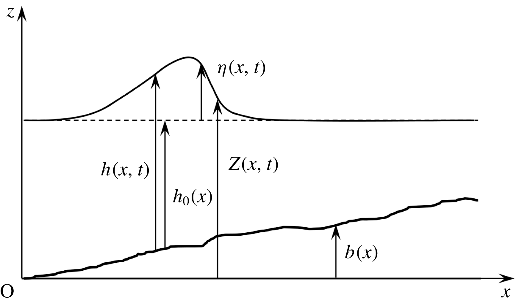
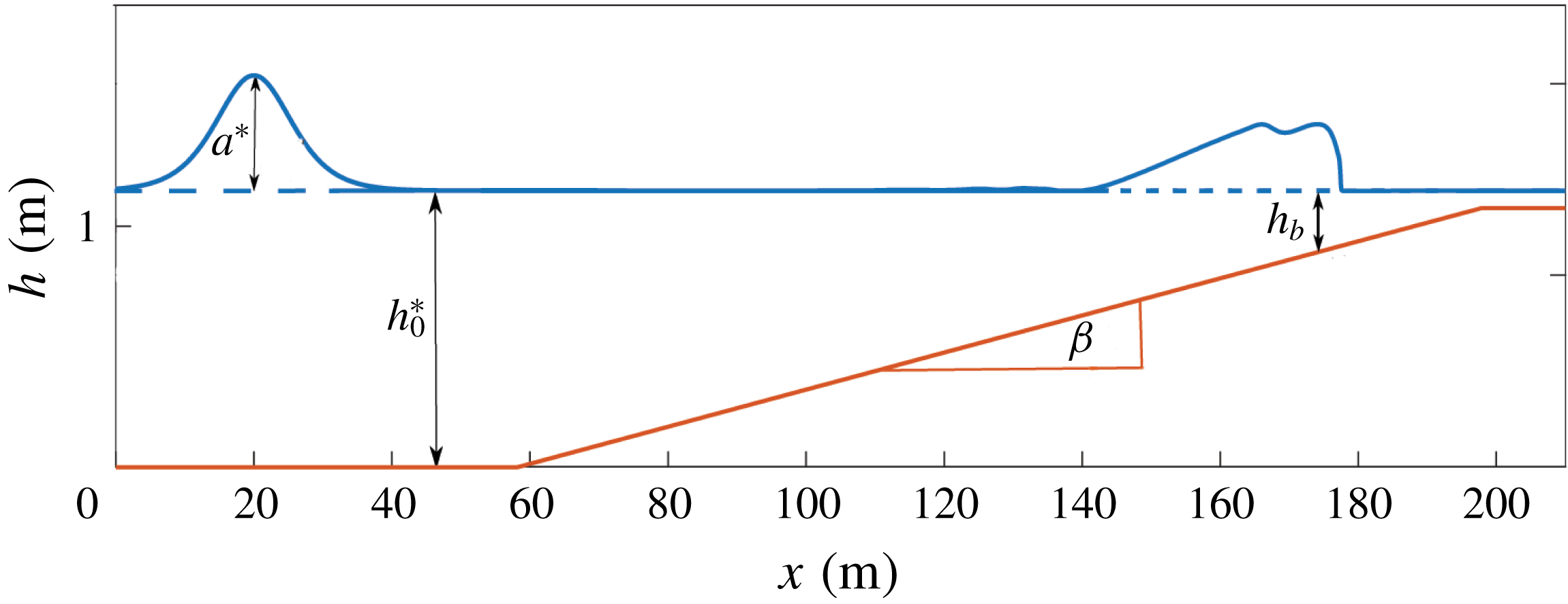
We study the particular case of a two-dimensional flow over a variable bottom. The notations are presented in figure 1. The components of the velocity field are
 $u$
in the horizontal direction
 $Ox$
and
 $w$
in the vertical direction
 $Oz$
. The bottom topography is measured by its elevation
 $b(x)$
over a horizontal datum.
Notations used in the text.

The free-surface location
 $h^{\ast }$
can be written as the sum of a filtered term
 $h$
and a residual term
 $h^{\prime }$
i.e.
 $h^{\ast }=h+h^{\prime }$
where the filtered free surface is a smooth mean free surface. The boundary conditions for the filtered flow at this mean surface were first derived for non-splashing regimes by Hasselmann (Reference Hasselmann1971) and extended to the case of splashing regimes with disconnected surfaces by Brocchini & Peregrine (Reference Brocchini and Peregrine2001) by a careful study of the two-phase surface layer. The major difficulty in using these turbulent boundary conditions is to find closures for the new terms and in particular for the turbulent stresses at the smooth surface. Approximate boundary conditions were derived by Brocchini (Reference Brocchini2002) in the case of a thin bubbly/weakly splashing surface layer.
These considerations can prove important in particular for non-hydrostatic models based on Reynolds-averaged Navier–Stokes equations as an underestimation of the turbulent viscosity was attributed to a zero-tangential-stress boundary condition imposed at the smooth free surface instead of these turbulent boundary conditions (Derakhti et al. Reference Derakhti, Kirby, Shi and Ma2016). It is of much less importance for depth-averaged models. Working on turbulent hydraulic jumps providing the best similarities with near-shore breaking waves, Svendsen et al. (Reference Svendsen, Veeramony, Bakunin and Kirby2000) stated that the terms due to the turbulent fluctuations of the free surface give negligible contributions and they omitted them in their integration over the depth. Measurements by laser Doppler anemometry by Stansby & Feng (Reference Stansby and Feng2005) on surf zone waves showed that the terms of the boundary conditions associated with the turbulent aerated two-phase flow at the air/water interface can be ignored, at least in an instantaneous depth-integrated sense. Accordingly very few depth-integrated models, if any, used these turbulent boundary conditions even those modelling turbulence such as the two-layer model of Gavrilyuk et al. (Reference Gavrilyuk, Liapidevskii and Chesnokov2016). In the same way, the semi-integrated model of Antuono & Brocchini (Reference Antuono and Brocchini2013) did not consider the turbulent contribution to the free-surface position and used the classical kinematic boundary condition and the shallow-water sloshing model of Antuono et al. (Reference Antuono, Bardazzi, Lugni and Brocchini2014) for wave breaking similarly neglected the turbulent stresses at the free surface. We do likewise in the derivation of our model by considering a smooth filtered free surface and by neglecting the residual stresses at the free surface. This proves to be sufficient to model correctly the dissipation effects in breaking waves within the framework of our depth-integrated model.
The elevation of the smooth filtered free surface over this horizontal datum is
 $Z(x,t)$
while the water depth is
 $h(x,t)=Z(x,t)-b(x)$
. The still water depth is denoted by
 $h_{0}(x)$
and the water elevation over this level is
 $\unicode[STIX]{x1D702}(x,t)$
. In the case of a solitary wave, the amplitude
 $a$
of the wave is defined as the maximum value of the elevation i.e.
 $a=\unicode[STIX]{x1D702}_{max}$
.
The filtered mass conservation equation is
 $$\begin{eqnarray}\frac{\unicode[STIX]{x2202}\overline{u}}{\unicode[STIX]{x2202}x}+\frac{\unicode[STIX]{x2202}\overline{w}}{\unicode[STIX]{x2202}z}=0.\end{eqnarray}$$
The filtered momentum balance equation writes in the
 $Ox$
direction
 $$\begin{eqnarray}\frac{\unicode[STIX]{x2202}\overline{u}}{\unicode[STIX]{x2202}t}+\frac{\unicode[STIX]{x2202}\overline{u}^{2}}{\unicode[STIX]{x2202}x}+\frac{\unicode[STIX]{x2202}\overline{u}\,\overline{w}}{\unicode[STIX]{x2202}z}=-\frac{1}{\unicode[STIX]{x1D70C}}\frac{\unicode[STIX]{x2202}p}{\unicode[STIX]{x2202}x}+\frac{1}{\unicode[STIX]{x1D70C}}\left(\frac{\unicode[STIX]{x2202}\unicode[STIX]{x1D608}_{xx}^{r}}{\unicode[STIX]{x2202}x}+\frac{\unicode[STIX]{x2202}\unicode[STIX]{x1D608}_{xz}^{r}}{\unicode[STIX]{x2202}z}\right)+\unicode[STIX]{x1D708}\left(\frac{\unicode[STIX]{x2202}^{2}u}{\unicode[STIX]{x2202}x^{2}}+\frac{\unicode[STIX]{x2202}^{2}u}{\unicode[STIX]{x2202}z^{2}}\right)\end{eqnarray}$$
and in the
 $Oz$
direction
 $$\begin{eqnarray}\frac{\unicode[STIX]{x2202}\overline{w}}{\unicode[STIX]{x2202}t}+\frac{\unicode[STIX]{x2202}\overline{u}\,\overline{w}}{\unicode[STIX]{x2202}x}+\frac{\unicode[STIX]{x2202}\overline{w}^{2}}{\unicode[STIX]{x2202}z}=-g-\frac{1}{\unicode[STIX]{x1D70C}}\frac{\unicode[STIX]{x2202}p}{\unicode[STIX]{x2202}z}+\frac{1}{\unicode[STIX]{x1D70C}}\left(\frac{\unicode[STIX]{x2202}\unicode[STIX]{x1D608}_{xz}^{r}}{\unicode[STIX]{x2202}x}+\frac{\unicode[STIX]{x2202}\unicode[STIX]{x1D608}_{zz}^{r}}{\unicode[STIX]{x2202}z}\right)+\unicode[STIX]{x1D708}\left(\frac{\unicode[STIX]{x2202}^{2}w}{\unicode[STIX]{x2202}x^{2}}+\frac{\unicode[STIX]{x2202}^{2}w}{\unicode[STIX]{x2202}z^{2}}\right).\end{eqnarray}$$
The balance equation for the kinetic energy of the filtered motions can be written
 $$\begin{eqnarray}\displaystyle & & \displaystyle \frac{\unicode[STIX]{x2202}}{\unicode[STIX]{x2202}t}\left(\frac{\overline{u}^{2}}{2}+\frac{\overline{w}^{2}}{2}\right)\nonumber\\ \displaystyle & & \displaystyle \qquad +\,\frac{\unicode[STIX]{x2202}}{\unicode[STIX]{x2202}x}\left[\overline{u}\left(\frac{\overline{u}^{2}}{2}+\frac{\overline{w}^{2}}{2}+gz\right)+\frac{pu}{\unicode[STIX]{x1D70C}}-\frac{\unicode[STIX]{x1D608}_{xx}^{r}u}{\unicode[STIX]{x1D70C}}-\frac{\unicode[STIX]{x1D608}_{xz}^{r}w}{\unicode[STIX]{x1D70C}}-\frac{\unicode[STIX]{x1D70F}_{xx}u}{\unicode[STIX]{x1D70C}}-\frac{\unicode[STIX]{x1D70F}_{xz}w}{\unicode[STIX]{x1D70C}}\right]\nonumber\\ \displaystyle & & \displaystyle \qquad +\,\frac{\unicode[STIX]{x2202}}{\unicode[STIX]{x2202}z}\left[\overline{w}\left(\frac{\overline{u}^{2}}{2}+\frac{\overline{w}^{2}}{2}+gz\right)+\frac{pw}{\unicode[STIX]{x1D70C}}-\frac{\unicode[STIX]{x1D608}_{xz}^{r}u}{\unicode[STIX]{x1D70C}}-\frac{\unicode[STIX]{x1D608}_{zz}^{r}w}{\unicode[STIX]{x1D70C}}-\frac{\unicode[STIX]{x1D70F}_{xz}u}{\unicode[STIX]{x1D70C}}-\frac{\unicode[STIX]{x1D70F}_{zz}w}{\unicode[STIX]{x1D70C}}\right]\nonumber\\ \displaystyle & & \displaystyle \quad =-\unicode[STIX]{x1D700}_{f}-P^{r}.\end{eqnarray}$$
In this equation, the filtered viscous stress tensor is
 $\unicode[STIX]{x1D749}=2\unicode[STIX]{x1D70C}\unicode[STIX]{x1D708}\overline{\unicode[STIX]{x1D63F}}$
. The components of the involved symmetrical tensors are defined as
 $\unicode[STIX]{x1D63C}^{r}=\unicode[STIX]{x1D608}_{xx}^{r}\boldsymbol{e}_{\boldsymbol{x}}\otimes \boldsymbol{e}_{\boldsymbol{x}}+\unicode[STIX]{x1D608}_{xz}^{r}\boldsymbol{e}_{\boldsymbol{x}}\otimes \boldsymbol{e}_{\boldsymbol{z}}+\unicode[STIX]{x1D608}_{xz}^{r}\boldsymbol{e}_{\boldsymbol{z}}\otimes \boldsymbol{e}_{\boldsymbol{x}}+\unicode[STIX]{x1D608}_{zz}^{r}\boldsymbol{e}_{\boldsymbol{z}}\otimes \boldsymbol{e}_{\boldsymbol{z}}$
and
 $\unicode[STIX]{x1D749}=\unicode[STIX]{x1D70F}_{xx}\boldsymbol{e}_{\boldsymbol{x}}\otimes \boldsymbol{e}_{\boldsymbol{x}}+\unicode[STIX]{x1D70F}_{xz}\boldsymbol{e}_{\boldsymbol{x}}\otimes \boldsymbol{e}_{\boldsymbol{z}}+\unicode[STIX]{x1D70F}_{xz}\boldsymbol{e}_{\boldsymbol{z}}\otimes \boldsymbol{e}_{\boldsymbol{x}}+\unicode[STIX]{x1D70F}_{zz}\boldsymbol{e}_{\boldsymbol{z}}\otimes \boldsymbol{e}_{\boldsymbol{z}}$
, where
 $\boldsymbol{e}_{\boldsymbol{x}}$
and
 $\boldsymbol{e}_{\boldsymbol{z}}$
are the unit vectors in the
 $Ox$
and
 $Oz$
directions.
The boundary conditions are the no-penetration condition at the bottom
 $$\begin{eqnarray}w(b)=u(b)b_{x},\end{eqnarray}$$
where
 $b_{x}=\text{d}b/\text{d}x$
, the kinematic boundary condition at the free surface
 $$\begin{eqnarray}w(Z)=\frac{\unicode[STIX]{x2202}h}{\unicode[STIX]{x2202}t}+u(Z)\frac{\unicode[STIX]{x2202}Z}{\unicode[STIX]{x2202}x}\end{eqnarray}$$
and the dynamic boundary condition at the free surface
 $$\begin{eqnarray}(\unicode[STIX]{x1D748}\boldsymbol{\cdot }\boldsymbol{n})(Z)=0,\end{eqnarray}$$
where
 $\unicode[STIX]{x1D748}=-p\unicode[STIX]{x1D644}+\unicode[STIX]{x1D63C}^{r}+\unicode[STIX]{x1D749}$
is the Cauchy stress tensor and where
 $\boldsymbol{n}$
is the unit normal vector at the free surface.
3.2 Scaling
The model is derived within the scope of the shallow-water approximation. If
 $h_{0}^{\ast }$
is a reference value of the still water depth and if
 $L$
is a characteristic length of variation of the flow parameters in the horizontal direction, then there is a small parameter
 $$\begin{eqnarray}\unicode[STIX]{x1D707}=\frac{h_{0}^{\ast }}{L}\ll 1.\end{eqnarray}$$
The equations are then written in dimensionless form. The dimensionless quantities are denoted by a tilde symbol. The following scaling is classical for this situation (Antuono & Brocchini Reference Antuono and Brocchini2013):
 $$\begin{eqnarray}\left.\begin{array}{@{}c@{}}\displaystyle \tilde{x}=\frac{x}{L};\quad \tilde{z}=\frac{z}{h_{0}^{\ast }};\quad \tilde{u} =\frac{\overline{u}}{\sqrt{gh_{0}^{\ast }}};\quad \tilde{w}=\frac{\overline{w}}{\unicode[STIX]{x1D707}\sqrt{gh_{0}^{\ast }}};\\ \displaystyle \tilde{t}=\unicode[STIX]{x1D707}t\sqrt{\frac{g}{h_{0}^{\ast }}};\quad \tilde{h}=\frac{h}{h_{0}^{\ast }};\quad \tilde{p}=\frac{p}{\unicode[STIX]{x1D70C}gh_{0}^{\ast }}.\end{array}\right\}\end{eqnarray}$$
For the viscous stress tensor, the scaling is
 $$\begin{eqnarray}\tilde{\unicode[STIX]{x1D70F}}_{xx}=\frac{L\unicode[STIX]{x1D70F}_{xx}}{\unicode[STIX]{x1D70C}\unicode[STIX]{x1D708}\sqrt{gh_{0}^{\ast }}};\quad \tilde{\unicode[STIX]{x1D70F}}_{zz}=\frac{L\unicode[STIX]{x1D70F}_{zz}}{\unicode[STIX]{x1D70C}\unicode[STIX]{x1D708}\sqrt{gh_{0}^{\ast }}};\quad \tilde{\unicode[STIX]{x1D70F}}_{xz}=\frac{\unicode[STIX]{x1D70F}_{xz}}{\unicode[STIX]{x1D70C}\unicode[STIX]{x1D708}}\sqrt{\frac{h_{0}^{\ast }}{g}}.\end{eqnarray}$$
The Reynolds number is defined by
 $Re=h_{0}^{\ast }\sqrt{gh_{0}^{\ast }}/\unicode[STIX]{x1D708}$
. Experimental measures on breaking waves (Cox, Kobayashi & Okayasu Reference Cox, Kobayashi and Okayasu1995) or turbulent hydraulic jumps similar to breaking waves (Svendsen et al.
Reference Svendsen, Veeramony, Bakunin and Kirby2000) showed that the ratio
 $\unicode[STIX]{x1D708}_{T}/(h_{0}^{\ast }\sqrt{gh_{0}^{\ast }})$
is small, of the order of
 $10^{-2}$
. Accordingly the turbulent viscosity is supposed to be of
 $O(\unicode[STIX]{x1D707})$
and it is written in dimensionless form as in Antuono & Brocchini (Reference Antuono and Brocchini2013) or in Zhang et al. (Reference Zhang, Kennedy, Donahue, Westerink, Panda and Dawson2014):
 $$\begin{eqnarray}\tilde{\unicode[STIX]{x1D708}}_{T}=\frac{\unicode[STIX]{x1D708}_{T}}{\unicode[STIX]{x1D707}h_{0}^{\ast }\sqrt{gh_{0}^{\ast }}}.\end{eqnarray}$$
Consequently the components of the deviatoric part of the residual stress tensor are scaled as
 $$\begin{eqnarray}\tilde{\unicode[STIX]{x1D608}}_{xx}^{r}=\frac{\unicode[STIX]{x1D608}_{xx}^{r}}{\unicode[STIX]{x1D707}^{2}\unicode[STIX]{x1D70C}gh_{0}^{\ast }};\quad \tilde{\unicode[STIX]{x1D608}}_{zz}^{r}=\frac{\unicode[STIX]{x1D608}_{zz}^{r}}{\unicode[STIX]{x1D707}^{2}\unicode[STIX]{x1D70C}gh_{0}^{\ast }};\quad \tilde{\unicode[STIX]{x1D608}}_{xz}^{r}=\frac{\unicode[STIX]{x1D608}_{xz}^{r}}{\unicode[STIX]{x1D707}\unicode[STIX]{x1D70C}gh_{0}^{\ast }}.\end{eqnarray}$$
We can write
 $$\begin{eqnarray}\tilde{\unicode[STIX]{x1D608}}_{xx}^{r}=2\tilde{\unicode[STIX]{x1D708}}_{T}\frac{\unicode[STIX]{x2202}\tilde{u} }{\unicode[STIX]{x2202}\tilde{x}};\quad \tilde{\unicode[STIX]{x1D608}}_{zz}^{r}=-\tilde{\unicode[STIX]{x1D608}}_{xx}^{r};\quad \tilde{\unicode[STIX]{x1D608}}_{xz}^{r}=\tilde{\unicode[STIX]{x1D708}}_{T}\left(\frac{\unicode[STIX]{x2202}\tilde{u} }{\unicode[STIX]{x2202}\tilde{z}}+\unicode[STIX]{x1D707}^{2}\frac{\unicode[STIX]{x2202}\tilde{w}}{\unicode[STIX]{x2202}\tilde{x}}\right).\end{eqnarray}$$
The dimensionless mass conservation equation is simply
 $$\begin{eqnarray}\frac{\unicode[STIX]{x2202}\tilde{u} }{\unicode[STIX]{x2202}\tilde{x}}+\frac{\unicode[STIX]{x2202}\tilde{w}}{\unicode[STIX]{x2202}\tilde{z}}=0.\end{eqnarray}$$
The momentum equation in the
 $Ox$
direction becomes in dimensionless form
 $$\begin{eqnarray}\frac{\unicode[STIX]{x2202}\tilde{u} }{\unicode[STIX]{x2202}\tilde{t}}+\frac{\unicode[STIX]{x2202}\tilde{u} ^{2}}{\unicode[STIX]{x2202}\tilde{x}}+\frac{\unicode[STIX]{x2202}\tilde{u} \tilde{w}}{\unicode[STIX]{x2202}\tilde{z}}=-\frac{\unicode[STIX]{x2202}\tilde{p}}{\unicode[STIX]{x2202}\tilde{x}}+\unicode[STIX]{x1D707}^{2}\frac{\unicode[STIX]{x2202}\tilde{\unicode[STIX]{x1D608}}_{xx}^{r}}{\unicode[STIX]{x2202}\tilde{x}}+\frac{\unicode[STIX]{x2202}\tilde{\unicode[STIX]{x1D608}}_{xz}^{r}}{\unicode[STIX]{x2202}\tilde{z}}+\frac{\unicode[STIX]{x1D707}}{Re}\frac{\unicode[STIX]{x2202}\tilde{\unicode[STIX]{x1D70F}}_{xx}}{\unicode[STIX]{x2202}\tilde{x}}+\frac{1}{\unicode[STIX]{x1D707}Re}\frac{\unicode[STIX]{x2202}\tilde{\unicode[STIX]{x1D70F}}_{xz}}{\unicode[STIX]{x2202}\tilde{z}}.\end{eqnarray}$$
In the
 $Oz$
direction, the momentum equation can be written
 $$\begin{eqnarray}\unicode[STIX]{x1D707}^{2}\left(\frac{\unicode[STIX]{x2202}\tilde{w}}{\unicode[STIX]{x2202}\tilde{t}}+\frac{\unicode[STIX]{x2202}\tilde{u} \tilde{w}}{\unicode[STIX]{x2202}\tilde{x}}+\frac{\unicode[STIX]{x2202}\tilde{w}^{2}}{\unicode[STIX]{x2202}\tilde{z}}\right)=-1-\frac{\unicode[STIX]{x2202}\tilde{p}}{\unicode[STIX]{x2202}\tilde{z}}+\unicode[STIX]{x1D707}^{2}\frac{\unicode[STIX]{x2202}\tilde{\unicode[STIX]{x1D608}}_{xz}^{r}}{\unicode[STIX]{x2202}\tilde{x}}+\unicode[STIX]{x1D707}^{2}\frac{\unicode[STIX]{x2202}\tilde{\unicode[STIX]{x1D608}}_{zz}^{r}}{\unicode[STIX]{x2202}\tilde{z}}+\frac{\unicode[STIX]{x1D707}}{Re}\frac{\unicode[STIX]{x2202}\tilde{\unicode[STIX]{x1D70F}}_{xz}}{\unicode[STIX]{x2202}\tilde{x}}+\frac{\unicode[STIX]{x1D707}}{Re}\frac{\unicode[STIX]{x2202}\tilde{\unicode[STIX]{x1D70F}}_{zz}}{\unicode[STIX]{x2202}\tilde{z}}.\end{eqnarray}$$
It follows from the chosen scaling that the dimensionless viscous dissipation in the filtered velocity field can be defined as
 $\tilde{\unicode[STIX]{x1D700}}_{f}=h_{0}^{\ast }\unicode[STIX]{x1D700}_{f}/(g\unicode[STIX]{x1D708})$
and that the dimensionless energy transfer toward the residual motion is
 $\tilde{P}^{r}=P^{r}/(\unicode[STIX]{x1D707}g\sqrt{gh_{0}^{\ast }})$
. The dimensionless energy equation can then be written
 $$\begin{eqnarray}\displaystyle & & \displaystyle \frac{\unicode[STIX]{x2202}}{\unicode[STIX]{x2202}\tilde{t}}\left(\frac{\tilde{u} ^{2}}{2}+\unicode[STIX]{x1D707}^{2}\frac{\tilde{w}^{2}}{2}\right)\nonumber\\ \displaystyle & & \displaystyle \qquad +\,\frac{\unicode[STIX]{x2202}}{\unicode[STIX]{x2202}\tilde{x}}\left[\tilde{u} \left(\frac{\tilde{u} ^{2}}{2}+\unicode[STIX]{x1D707}^{2}\frac{\tilde{w}^{2}}{2}+\tilde{z}\right)+\tilde{p}\tilde{u} -\unicode[STIX]{x1D707}^{2}\left(\tilde{\unicode[STIX]{x1D608}}_{xx}^{r}\tilde{u} +\tilde{\unicode[STIX]{x1D608}}_{xz}^{r}\tilde{w}\right)-\frac{\unicode[STIX]{x1D707}}{Re}\left(\tilde{\unicode[STIX]{x1D70F}}_{xx}\tilde{u} +\tilde{\unicode[STIX]{x1D70F}}_{xz}\tilde{w}\right)\right]\nonumber\\ \displaystyle & & \displaystyle \qquad +\,\frac{\unicode[STIX]{x2202}}{\unicode[STIX]{x2202}\tilde{z}}\left[\tilde{w}\left(\frac{\tilde{u} ^{2}}{2}+\unicode[STIX]{x1D707}^{2}\frac{\tilde{w}^{2}}{2}+\tilde{z}\right)+\tilde{p}\tilde{w}-\tilde{\unicode[STIX]{x1D608}}_{xz}^{r}\tilde{u} -\unicode[STIX]{x1D707}^{2}\tilde{\unicode[STIX]{x1D608}}_{zz}^{r}\tilde{w}-\frac{1}{\unicode[STIX]{x1D707}Re}\tilde{\unicode[STIX]{x1D70F}}_{xz}\tilde{u} -\frac{\unicode[STIX]{x1D707}}{Re}\tilde{\unicode[STIX]{x1D70F}}_{zz}\tilde{w}\right]\nonumber\\ \displaystyle & & \displaystyle \quad =-\frac{1}{\unicode[STIX]{x1D707}Re}\tilde{\unicode[STIX]{x1D700}}_{f}-\tilde{P}^{r}.\end{eqnarray}$$
The boundary conditions are also written in dimensionless form with
 $\tilde{b}=b/h_{0}^{\ast }$
and
 $\tilde{Z}=Z/h_{0}^{\ast }$
. If we assume that
 $b$
varies horizontally on a characteristic length of
 $O(L)$
, then
 $\tilde{b}_{x}=b_{x}/\unicode[STIX]{x1D707}$
. The no-penetration condition on the bottom and the kinematic condition at the free surface write simply
 $$\begin{eqnarray}\tilde{w}(b)=\tilde{u} (b)\tilde{b}_{x};\quad \tilde{w}(Z)=\frac{\unicode[STIX]{x2202}\tilde{h}}{\unicode[STIX]{x2202}\tilde{t}}+\tilde{u} (Z)\frac{\unicode[STIX]{x2202}\tilde{Z}}{\unicode[STIX]{x2202}\tilde{x}},\end{eqnarray}$$
whereas the dynamic boundary condition at the free surface (3.7) gives two scalar equations
 $$\begin{eqnarray}\displaystyle & \displaystyle \tilde{\unicode[STIX]{x1D608}}_{xz}^{r}(Z)+[\tilde{p}(Z)-\unicode[STIX]{x1D707}^{2}\tilde{\unicode[STIX]{x1D608}}_{xx}^{r}(Z)]\frac{\unicode[STIX]{x2202}\tilde{Z}}{\unicode[STIX]{x2202}\tilde{x}}=0 & \displaystyle\end{eqnarray}$$
 $$\begin{eqnarray}\displaystyle & \displaystyle \tilde{p}(Z)-\unicode[STIX]{x1D707}^{2}\tilde{\unicode[STIX]{x1D608}}_{zz}^{r}(Z)+\unicode[STIX]{x1D707}^{2}\tilde{\unicode[STIX]{x1D608}}_{xz}^{r}(Z)\frac{\unicode[STIX]{x2202}\tilde{Z}}{\unicode[STIX]{x2202}\tilde{x}}=0. & \displaystyle\end{eqnarray}$$
There is no surface tension and no shear stress condition imposed at the free surface.
The filtered equations are averaged over the depth. For any quantity
 $A$
, its average value over the depth is denoted by
 $\langle \!\langle A\rangle \!\rangle$
and defined as
 $$\begin{eqnarray}\langle \!\langle A\rangle \!\rangle =\frac{1}{h}\int _{b(x)}^{Z(x,t)}A\,\text{d}z.\end{eqnarray}$$
The averaged horizontal velocity is denoted by
 $U=\langle \!\langle \overline{u}\rangle \!\rangle$
and in dimensionless form
 $\tilde{U} =\langle \!\langle \tilde{u} \rangle \!\rangle$
. As explained at the beginning of § 3.1, we consider a smooth free surface and we neglect all effects due to the turbulent contribution to the free-surface location. It follows that the upper limit of the integral defining the averaging over the depth (3.21) is taken at this smooth free surface. The filtered horizontal velocity is decomposed as
 $$\begin{eqnarray}\overline{u}(x,z,t)=U(x,t)+u^{\prime }(x,z,t).\end{eqnarray}$$
Equivalently,
 $u=U+u^{\prime }+u^{r}$
. The term
 $u^{\prime }$
represents the deviation of the filtered horizontal velocity from its averaged value. It includes the anisotropic large-scale turbulence which contains most of the turbulent energy and the depth variations of the Reynolds-averaged velocity field (shearing effects). On the other hand, the residual velocity field
 $u^{r}$
includes the isotropic small-scale turbulence where most of the dissipation takes place.
The model is derived in the hypothesis of a weakly turbulent (and weakly sheared) flow which means that
 $u^{\prime }$
is of
 $O(\unicode[STIX]{x1D707})$
. This hypothesis is very similar in effect as the hypothesis of a weakly sheared flow (Teshukov Reference Teshukov2007) with a value of Teshukov’s exponent
 $\unicode[STIX]{x1D6FD}$
equal to 1. Therefore we write
 $$\begin{eqnarray}\tilde{u} (x,z,t)=\tilde{U} (x,t)+\unicode[STIX]{x1D707}\tilde{u} ^{\prime }(x,z,t).\end{eqnarray}$$
In the following derivation of the model, all terms of an order up to
 $O(\unicode[STIX]{x1D707}^{2})$
will be kept and the terms of
 $O(\unicode[STIX]{x1D707}^{3})$
will be neglected.
In spite of its name, the assumption of a weakly turbulent flow does not prevent the application of the model to breaking waves with an intense turbulence. This same assumption was used by Richard & Gavrilyuk (Reference Richard and Gavrilyuk2013) to model turbulent hydraulic jumps in the framework of a hyperbolic non-dispersive model. The results of this model are in a very good agreement with the experimental results of Chanson (Reference Chanson2011) including for hydraulic jumps with an upstream Froude number of 8.25 that indicates an intense turbulence and which gives a ratio between maximum and minimum depths much higher than the depth ratios between trough and crest for surf zone waves (see Svendsen et al. Reference Svendsen, Veeramony, Bakunin and Kirby2000). This assumption entails no practical limitation to the study of highly turbulent breaking waves. It was also used similarly by Castro & Lannes (Reference Castro and Lannes2014) and by Gavrilyuk et al. (Reference Gavrilyuk, Liapidevskii and Chesnokov2016).
The Reynolds number is supposed to be high enough so that all viscous terms can be neglected. This hypothesis is usual for this kind of problem (see for example Antuono & Brocchini Reference Antuono and Brocchini2013). It can be written
 $Re=O(\unicode[STIX]{x1D707}^{-3})$
. The terms of
 $O(\unicode[STIX]{x1D707}/Re)$
are then of
 $O(\unicode[STIX]{x1D707}^{4})$
. The terms of
 $O(1/(\unicode[STIX]{x1D707}Re))$
involve
 $\tilde{\unicode[STIX]{x1D70F}}_{xz}$
whose dominant term is
 $\unicode[STIX]{x2202}\tilde{u} /\unicode[STIX]{x2202}\tilde{z}$
. Since
 $\unicode[STIX]{x2202}\tilde{U} /\unicode[STIX]{x2202}\tilde{z}=0$
,
 $\tilde{\unicode[STIX]{x1D70F}}_{xz}$
is in fact of
 $O(\unicode[STIX]{x1D707})$
and the terms of
 $O(1/(\unicode[STIX]{x1D707}Re))$
are of
 $O(\unicode[STIX]{x1D707}^{3})$
and therefore negligible. The term
 $\tilde{\unicode[STIX]{x1D700}}_{f}$
is negligible for the same reason.
The effect of the hypothesis of a weakly turbulent flow can also be applied to the scaling of
 $\overline{\unicode[STIX]{x1D63F}}$
and
 $P^{r}$
. In
 $\overline{\unicode[STIX]{x1D63F}}$
the dominant component is normally, in dimensionless form
 $$\begin{eqnarray}\tilde{\unicode[STIX]{x1D60B}}_{xz}=\frac{1}{2}\left(\frac{\unicode[STIX]{x2202}\tilde{u} }{\unicode[STIX]{x2202}\tilde{z}}+\unicode[STIX]{x1D707}^{2}\frac{\unicode[STIX]{x2202}\tilde{w}}{\unicode[STIX]{x2202}\tilde{x}}\right).\end{eqnarray}$$
However,
 $\unicode[STIX]{x2202}\tilde{u} /\unicode[STIX]{x2202}\tilde{z}=\unicode[STIX]{x1D707}\unicode[STIX]{x2202}\tilde{u} ^{\prime }/\unicode[STIX]{x2202}\tilde{z}$
. This implies that
 $$\begin{eqnarray}\tilde{P}^{r}=\frac{P^{r}}{\unicode[STIX]{x1D707}^{3}g\sqrt{gh_{0}^{\ast }}}.\end{eqnarray}$$
Consequently, the last term in (3.17) writes in fact
 $-\unicode[STIX]{x1D707}^{2}\tilde{P}^{r}$
. It is thus of
 $O(\unicode[STIX]{x1D707}^{2})$
and must be kept.
As in Veeramony & Svendsen (Reference Veeramony and Svendsen2000), the shear stress on the bottom is neglected and this implies a free-slip condition at the sea bed. The whole deviatoric residual stress tensor is neglected on the bottom i.e.
 $\unicode[STIX]{x1D63C}^{r}(b)\simeq 0$
. The shear stress on the bottom could be modelled by a classical drag term if needed such as a Chézy-type sea bed friction.
3.3 Averaging procedure
To lighten the notations, the tilde are dropped in this section dealing entirely with dimensionless quantities. Averaging the mass conservation equation (3.14) over the depth, taking into account the boundary conditions, gives
 $$\begin{eqnarray}\frac{\unicode[STIX]{x2202}h}{\unicode[STIX]{x2202}t}+\frac{\unicode[STIX]{x2202}hU}{\unicode[STIX]{x2202}x}=0.\end{eqnarray}$$
The continuity equation (3.14) allows us to find an expression for the vertical filtered velocity
 $$\begin{eqnarray}w=(z-b)\frac{\dot{h}}{h}+Ub_{x}+O(\unicode[STIX]{x1D707}),\end{eqnarray}$$
where the dot symbol denotes the material derivative along the average flow
 $$\begin{eqnarray}\dot{h}=\frac{\unicode[STIX]{x2202}h}{\unicode[STIX]{x2202}t}+U\frac{\unicode[STIX]{x2202}h}{\unicode[STIX]{x2202}x}=-h\frac{\unicode[STIX]{x2202}U}{\unicode[STIX]{x2202}x}.\end{eqnarray}$$
In the following we will denote by
 $\ddot{h}$
the material derivative of
 ${\dot{h}}$
along the average flow i.e.
 $$\begin{eqnarray}\ddot{h}={\displaystyle \frac{\unicode[STIX]{x2202}{\dot{h}}}{\unicode[STIX]{x2202}t}}+U{\displaystyle \frac{\unicode[STIX]{x2202}{\dot{h}}}{\unicode[STIX]{x2202}x}}=h\left({\displaystyle \frac{\unicode[STIX]{x2202}U}{\unicode[STIX]{x2202}x}}\right)^{2}-h{\displaystyle \frac{\unicode[STIX]{x2202}^{2}U}{\unicode[STIX]{x2202}x\unicode[STIX]{x2202}t}}-hU{\displaystyle \frac{\unicode[STIX]{x2202}^{2}U}{\unicode[STIX]{x2202}x^{2}}}.\end{eqnarray}$$
The momentum equation in the
 $Oz$
direction (3.16) gives first
 $$\begin{eqnarray}\frac{\unicode[STIX]{x2202}p}{\unicode[STIX]{x2202}z}=-1-\unicode[STIX]{x1D707}^{2}(z-b)\frac{\ddot{h}}{h}-\unicode[STIX]{x1D707}^{2}\frac{\text{D}b_{x}U}{\text{D}t}+\unicode[STIX]{x1D707}^{2}\frac{\unicode[STIX]{x2202}\unicode[STIX]{x1D608}_{xz}^{r}}{\unicode[STIX]{x2202}x}+\unicode[STIX]{x1D707}^{2}\frac{\unicode[STIX]{x2202}\unicode[STIX]{x1D608}_{zz}^{r}}{\unicode[STIX]{x2202}z}\end{eqnarray}$$
and then, with the dynamic boundary condition (3.20), an expression of the pressure
 $$\begin{eqnarray}\displaystyle p & = & \displaystyle Z-z-\unicode[STIX]{x1D707}^{2}\frac{\ddot{h}}{h}\left[\frac{z^{2}-Z^{2}}{2}-b(z-Z)\right]-\unicode[STIX]{x1D707}^{2}\frac{\text{D}b_{x}U}{\text{D}t}(z-Z)\nonumber\\ \displaystyle & & \displaystyle +\,\unicode[STIX]{x1D707}^{2}\frac{\unicode[STIX]{x2202}}{\unicode[STIX]{x2202}x}\int _{Z}^{z}\unicode[STIX]{x1D608}_{xz}^{r}\,\text{d}z+\unicode[STIX]{x1D707}^{2}\unicode[STIX]{x1D608}_{zz}^{r}.\end{eqnarray}$$
In these expressions, both the notations
 $\text{D}a/\text{D}t$
and
 ${\dot{a}}$
denote the material derivative of a quantity
 $a$
along the average flow (see (3.28)). With the dynamic boundary condition (3.19) and since we took
 $\unicode[STIX]{x1D63C}^{r}(b)\simeq 0$
, the integration of the pressure terms and of the residual stress terms gives
 $$\begin{eqnarray}\displaystyle & & \displaystyle -\int _{b}^{Z}\frac{\unicode[STIX]{x2202}p}{\unicode[STIX]{x2202}x}\,\text{d}z+\int _{b}^{Z}\unicode[STIX]{x1D707}^{2}\frac{\unicode[STIX]{x2202}\unicode[STIX]{x1D608}_{xx}^{r}}{\unicode[STIX]{x2202}x}\,\text{d}z+\int _{b}^{Z}\frac{\unicode[STIX]{x2202}\unicode[STIX]{x1D608}_{xz}^{r}}{\unicode[STIX]{x2202}z}\,\text{d}z\nonumber\\ \displaystyle & & \displaystyle \quad =-\frac{\unicode[STIX]{x2202}}{\unicode[STIX]{x2202}x}\int _{b}^{Z}p\,\text{d}z-p(b)b_{x}+\unicode[STIX]{x1D707}^{2}\frac{\unicode[STIX]{x2202}}{\unicode[STIX]{x2202}x}\int _{b}^{Z}\unicode[STIX]{x1D608}_{xx}^{r}\,\text{d}z.\end{eqnarray}$$
The integration of the pressure leads to
 $$\begin{eqnarray}\int _{b}^{Z}p\,\text{d}z=\frac{h^{2}}{2}+\unicode[STIX]{x1D707}^{2}\frac{h^{2}\ddot{h}}{3}+\unicode[STIX]{x1D707}^{2}\frac{h^{2}}{2}\frac{\text{D}b_{x}U}{\text{D}t}+\unicode[STIX]{x1D707}^{2}\int _{b}^{Z}\text{d}z\frac{\unicode[STIX]{x2202}}{\unicode[STIX]{x2202}x}\int _{Z}^{z}\unicode[STIX]{x1D608}_{xz}^{r}\,\text{d}z+\unicode[STIX]{x1D707}^{2}\int _{b}^{Z}\unicode[STIX]{x1D608}_{zz}^{r}\,\text{d}z.\end{eqnarray}$$
We can write
 $$\begin{eqnarray}\int _{Z}^{z}\unicode[STIX]{x1D608}_{xz}^{r}\,\text{d}z=\int _{Z}^{z}\unicode[STIX]{x1D708}_{T}\frac{\unicode[STIX]{x2202}u}{\unicode[STIX]{x2202}z}\,\text{d}z+O(\unicode[STIX]{x1D707}^{2}).\end{eqnarray}$$
Since the turbulent viscosity is uniform over the fluid depth,
 $$\begin{eqnarray}\int _{Z}^{z}\unicode[STIX]{x1D708}_{T}\frac{\unicode[STIX]{x2202}u}{\unicode[STIX]{x2202}z}\,\text{d}z=\unicode[STIX]{x1D708}_{T}(u-u(Z)).\end{eqnarray}$$
The hypothesis of a weakly turbulent flow implies that
 $u-u(Z)=O(\unicode[STIX]{x1D707})$
. The corresponding term in (3.33) is thus of
 $O(\unicode[STIX]{x1D707}^{3})$
and negligible. Then
 $$\begin{eqnarray}\int _{b}^{Z}\unicode[STIX]{x1D608}_{xx}^{r}\,\text{d}z=-\int _{b}^{Z}\unicode[STIX]{x1D608}_{zz}^{r}\,\text{d}z.\end{eqnarray}$$
With the expression of
 $\unicode[STIX]{x1D608}_{xx}^{r}$
, we get
 $$\begin{eqnarray}\int _{b}^{Z}\unicode[STIX]{x1D608}_{xx}^{r}\,\text{d}z=2\unicode[STIX]{x1D708}_{T}\int _{b}^{Z}\frac{\unicode[STIX]{x2202}u}{\unicode[STIX]{x2202}x}\,\text{d}z.\end{eqnarray}$$
The hypothesis of a weakly turbulent flow allows us to write
 $u(Z)=U+O(\unicode[STIX]{x1D707})$
and
 $u(b)=U+O(\unicode[STIX]{x1D707})$
. This leads to
 $$\begin{eqnarray}\int _{b}^{Z}\unicode[STIX]{x1D608}_{xx}^{r}\,\text{d}z=2\unicode[STIX]{x1D708}_{T}h\frac{\unicode[STIX]{x2202}U}{\unicode[STIX]{x2202}x}+O(\unicode[STIX]{x1D707}).\end{eqnarray}$$
The calculation of the pressure at the sea bed gives
 $$\begin{eqnarray}p(b)b_{x}=hb_{x}+\unicode[STIX]{x1D707}^{2}hb_{x}\left(\frac{\ddot{h}}{2}+\frac{\text{D}b_{x}U}{\text{D}t}\right).\end{eqnarray}$$
Finally the integration of the right-hand side of (3.15) gives
 $$\begin{eqnarray}\displaystyle & & \displaystyle -\int _{b}^{Z}\frac{\unicode[STIX]{x2202}p}{\unicode[STIX]{x2202}x}\,\text{d}z+\int _{b}^{Z}\unicode[STIX]{x1D707}^{2}\frac{\unicode[STIX]{x2202}\unicode[STIX]{x1D608}_{xx}^{r}}{\unicode[STIX]{x2202}x}\,\text{d}z+\int _{b}^{Z}\frac{\unicode[STIX]{x2202}\unicode[STIX]{x1D608}_{xz}^{r}}{\unicode[STIX]{x2202}z}\,\text{d}z\nonumber\\ \displaystyle & & \displaystyle \quad =-\frac{\unicode[STIX]{x2202}}{\unicode[STIX]{x2202}x}\left[\frac{h^{2}}{2}+\unicode[STIX]{x1D707}^{2}\left(\frac{h^{2}\ddot{h}}{3}+\frac{h^{2}}{2}\frac{\text{D}b_{x}U}{\text{D}t}-4\unicode[STIX]{x1D708}_{T}h\frac{\unicode[STIX]{x2202}U}{\unicode[STIX]{x2202}x}\right)\right]-hb_{x}-\unicode[STIX]{x1D707}^{2}hb_{x}\left(\frac{\ddot{h}}{2}+\frac{\text{D}b_{x}U}{\text{D}t}\right).\nonumber\\ \displaystyle & & \displaystyle\end{eqnarray}$$
Taking into account the boundary conditions, the integration of the left-hand side of (3.15) leads to
 $$\begin{eqnarray}\int _{b}^{Z}\left(\frac{\unicode[STIX]{x2202}u}{\unicode[STIX]{x2202}t}+\frac{\unicode[STIX]{x2202}u^{2}}{\unicode[STIX]{x2202}x}+\frac{\unicode[STIX]{x2202}uw}{\unicode[STIX]{x2202}z}\right)\text{d}z=\frac{\unicode[STIX]{x2202}hU}{\unicode[STIX]{x2202}t}+\frac{\unicode[STIX]{x2202}}{\unicode[STIX]{x2202}x}(h\langle \!\langle u^{2}\rangle \!\rangle ).\end{eqnarray}$$
The treatment of
 $\langle \!\langle u^{2}\rangle \!\rangle$
is the same as in Richard & Gavrilyuk (Reference Richard and Gavrilyuk2012). First,
 $\langle \!\langle u^{2}\rangle \!\rangle$
is written
 $U^{2}+\unicode[STIX]{x1D707}^{2}\langle \!\langle u^{\prime 2}\rangle \!\rangle$
since, by definition,
 $\langle \!\langle u^{\prime }\rangle \!\rangle =0$
. Second, a new variable, called enstrophy, is defined as
 $$\begin{eqnarray}\unicode[STIX]{x1D711}=\frac{\langle \!\langle u^{\prime 2}\rangle \!\rangle }{h^{2}}.\end{eqnarray}$$
The averaged momentum equation can finally be written
 $$\begin{eqnarray}\frac{\unicode[STIX]{x2202}hU}{\unicode[STIX]{x2202}t}+\frac{\unicode[STIX]{x2202}}{\unicode[STIX]{x2202}x}\left(hU^{2}+\unicode[STIX]{x1D707}^{2}h^{3}\unicode[STIX]{x1D711}+\frac{h^{2}}{2}+\unicode[STIX]{x1D707}^{2}\unicode[STIX]{x1D6F1}+\unicode[STIX]{x1D707}^{2}\unicode[STIX]{x1D6F1}^{\prime }\right)=-hb_{x}-\unicode[STIX]{x1D707}^{2}f^{\prime }+O(\unicode[STIX]{x1D707}^{3}),\end{eqnarray}$$
where
 $$\begin{eqnarray}\displaystyle & \displaystyle \unicode[STIX]{x1D6F1}=\frac{h^{2}\ddot{h}}{3}-4\unicode[STIX]{x1D708}_{T}h\frac{\unicode[STIX]{x2202}U}{\unicode[STIX]{x2202}x}, & \displaystyle\end{eqnarray}$$
 $$\begin{eqnarray}\displaystyle & \displaystyle \unicode[STIX]{x1D6F1}^{\prime }=\frac{h^{2}}{2}\frac{\text{D}b_{x}U}{\text{D}t} & \displaystyle\end{eqnarray}$$
and
 $$\begin{eqnarray}f^{\prime }=hb_{x}\left(\frac{\ddot{h}}{2}+\frac{\text{D}b_{x}U}{\text{D}t}\right)\!.\end{eqnarray}$$
We will say that the sea bed has a mild slope if
 $b$
varies horizontally on a characteristic length of
 $O(L/\unicode[STIX]{x1D707})$
. In this case, the terms in
 $\unicode[STIX]{x1D707}^{2}\unicode[STIX]{x1D6F1}^{\prime }$
and
 $-\unicode[STIX]{x1D707}^{2}f^{\prime }$
become of
 $O(\unicode[STIX]{x1D707}^{3})$
and are negligible. The averaged momentum equation reduces to
 $$\begin{eqnarray}\frac{\unicode[STIX]{x2202}hU}{\unicode[STIX]{x2202}t}+\frac{\unicode[STIX]{x2202}}{\unicode[STIX]{x2202}x}\left(hU^{2}+\unicode[STIX]{x1D707}^{2}h^{3}\unicode[STIX]{x1D711}+\frac{h^{2}}{2}+\unicode[STIX]{x1D707}^{2}\frac{h^{2}\ddot{h}}{3}-\unicode[STIX]{x1D707}^{2}4\unicode[STIX]{x1D708}_{T}h\frac{\unicode[STIX]{x2202}U}{\unicode[STIX]{x2202}x}\right)=-\unicode[STIX]{x1D707}hb_{x}+O(\unicode[STIX]{x1D707}^{3}).\end{eqnarray}$$
The conservative hyperbolic part of this equation was first derived by Teshukov (Reference Teshukov2007) in the general 2-D case and the dispersive term was studied in Castro & Lannes (Reference Castro and Lannes2014). The viscous term is new in this context. Since the model features three variables
 $h$
,
 $U$
and
 $\unicode[STIX]{x1D711}$
, three equations are needed. Two equations are provided by the averaged mass conservation equation and by the averaged momentum equation and the third equation is the averaged energy equation. With the boundary conditions, we can integrate
 $$\begin{eqnarray}\int _{b}^{Z}\left[\frac{\unicode[STIX]{x2202}}{\unicode[STIX]{x2202}t}\frac{u^{2}}{2}+\frac{\unicode[STIX]{x2202}}{\unicode[STIX]{x2202}x}\frac{u^{3}}{2}+\frac{\unicode[STIX]{x2202}}{\unicode[STIX]{x2202}z}\frac{wu^{2}}{2}\right]\text{d}z=\frac{\unicode[STIX]{x2202}}{\unicode[STIX]{x2202}t}\left(\frac{h}{2}\langle \!\langle u^{2}\rangle \!\rangle \right)+\frac{\unicode[STIX]{x2202}}{\unicode[STIX]{x2202}x}\left(\frac{h}{2}\langle \!\langle u^{3}\rangle \!\rangle \right)\!.\end{eqnarray}$$
We can expand as above
 $\langle \!\langle u^{2}\rangle \!\rangle =U^{2}+\unicode[STIX]{x1D707}^{2}h^{2}\unicode[STIX]{x1D711}$
. The same method yields
 $\langle \!\langle u^{3}\rangle \!\rangle =U^{3}+3\unicode[STIX]{x1D707}^{2}h^{2}U\unicode[STIX]{x1D711}+O(\unicode[STIX]{x1D707}^{3})$
. As in Teshukov (Reference Teshukov2007), the hypothesis of weakly turbulent flows allows us to neglect
 $\langle \!\langle {u^{\prime }}^{3}\rangle \!\rangle$
and thus to close the problem. Another integration combined with the boundary conditions and with the expression (3.27) of the vertical velocity leads to
 $$\begin{eqnarray}\displaystyle & & \displaystyle \!\!\!\!\displaystyle \unicode[STIX]{x1D707}^{2}\int _{b}^{Z}\left[\frac{\unicode[STIX]{x2202}}{\unicode[STIX]{x2202}t}\frac{w^{2}}{2}+\frac{\unicode[STIX]{x2202}}{\unicode[STIX]{x2202}x}\frac{uw^{2}}{2}+\frac{\unicode[STIX]{x2202}}{\unicode[STIX]{x2202}z}\frac{w^{3}}{2}\right]\text{d}z\nonumber\\ \displaystyle & & \displaystyle \!\!\!\!\quad =\unicode[STIX]{x1D707}^{2}\frac{\unicode[STIX]{x2202}}{\unicode[STIX]{x2202}t}\left(\frac{h{\dot{h}}^{2}}{6}+\frac{hU^{2}b_{x}^{2}}{2}+\frac{hb_{x}U{\dot{h}}}{2}\right)+\unicode[STIX]{x1D707}^{2}\frac{\unicode[STIX]{x2202}}{\unicode[STIX]{x2202}x}\left[U\!\left(\frac{h{\dot{h}}^{2}}{6}+\frac{hU^{2}b_{x}^{2}}{2}+\frac{hb_{x}U{\dot{h}}}{2}\right)\right]\!.\;\qquad \;\end{eqnarray}$$
With the expression (3.31) of the pressure and with the boundary conditions, we get
 $$\begin{eqnarray}\displaystyle & & \displaystyle \!\!\!\!\int _{b}^{Z}\left[\frac{\unicode[STIX]{x2202}}{\unicode[STIX]{x2202}x}(uz+pu-\unicode[STIX]{x1D707}^{2}\unicode[STIX]{x1D608}_{xx}^{r}u-\unicode[STIX]{x1D707}^{2}\unicode[STIX]{x1D608}_{xz}^{r}w)+\frac{\unicode[STIX]{x2202}}{\unicode[STIX]{x2202}z}(wz+pw-\unicode[STIX]{x1D608}_{xz}^{r}u-\unicode[STIX]{x1D707}^{2}\unicode[STIX]{x1D608}_{zz}^{r}w)\right]\text{d}z\nonumber\\ \displaystyle & & \displaystyle \!\!\!\!\quad =\frac{\unicode[STIX]{x2202}}{\unicode[STIX]{x2202}t}\left(\frac{h^{2}}{2}\right)+\frac{\unicode[STIX]{x2202}}{\unicode[STIX]{x2202}x}\left[U\!\left(h^{2}+\unicode[STIX]{x1D707}^{2}\frac{h^{2}\ddot{h}}{3}+\unicode[STIX]{x1D707}^{2}\frac{h^{2}}{2}\frac{\text{D}b_{x}U}{\text{D}t}-\unicode[STIX]{x1D707}^{2}4\unicode[STIX]{x1D708}_{T}h\frac{\unicode[STIX]{x2202}U}{\unicode[STIX]{x2202}x}\right)\right]+hb_{x}U\!.\;\qquad\end{eqnarray}$$
The averaged value of
 $P^{r}$
over the depth is estimated by the averaged value over the depth of its mean value (in the Reynolds sense)
 $\langle P^{r}\rangle$
. Then the approximation (2.17) gives
 $$\begin{eqnarray}\langle \!\langle P^{r}\rangle \!\rangle \simeq \langle \!\langle \unicode[STIX]{x1D700}\rangle \!\rangle .\end{eqnarray}$$
Physically, this means that the energy dissipation of the model is mostly due to the dissipation of the turbulent kinetic energy in the dissipation range i.e. in the small scales. The expression of
 $\langle \!\langle \unicode[STIX]{x1D700}\rangle \!\rangle$
is discussed in § 4. The averaged energy equation can finally be written
 $$\begin{eqnarray}\displaystyle & & \displaystyle \frac{\unicode[STIX]{x2202}}{\unicode[STIX]{x2202}t}[h(e+\unicode[STIX]{x1D707}^{2}e^{\prime })]+\frac{\unicode[STIX]{x2202}}{\unicode[STIX]{x2202}x}\left[hU(e+\unicode[STIX]{x1D707}^{2}e^{\prime })+U\left(\unicode[STIX]{x1D707}^{2}h^{3}\unicode[STIX]{x1D711}+\frac{h^{2}}{2}+\unicode[STIX]{x1D707}^{2}\unicode[STIX]{x1D6F1}+\unicode[STIX]{x1D707}^{2}\unicode[STIX]{x1D6F1}^{\prime }\right)\right]\nonumber\\ \displaystyle & & \displaystyle \quad =-hb_{x}U-\unicode[STIX]{x1D707}^{2}h\langle \!\langle \unicode[STIX]{x1D700}\rangle \!\rangle +O(\unicode[STIX]{x1D707}^{3}),\end{eqnarray}$$
where
 $\unicode[STIX]{x1D6F1}$
and
 $\unicode[STIX]{x1D6F1}^{\prime }$
are given by (3.44) and (3.45) respectively and where
 $$\begin{eqnarray}e=\frac{U^{2}}{2}+\unicode[STIX]{x1D707}^{2}\frac{h^{2}\unicode[STIX]{x1D711}}{2}+\unicode[STIX]{x1D707}^{2}\frac{{\dot{h}}^{2}}{6}+\frac{h}{2};\quad e^{\prime }=\frac{b_{x}^{2}U^{2}}{2}+\frac{{\dot{h}}}{2}b_{x}U.\end{eqnarray}$$
The factor
 $\unicode[STIX]{x1D707}^{2}$
in front of
 $h\langle \!\langle \unicode[STIX]{x1D700}\rangle \!\rangle$
comes from the hypothesis of a weakly turbulent flow as explained at the end of § 3.2 (see relation (3.25)). In the case of a mild slope,
 $e^{\prime }$
and
 $\unicode[STIX]{x1D6F1}^{\prime }$
become negligible and the energy equation reduces to
 $$\begin{eqnarray}\displaystyle \frac{\unicode[STIX]{x2202}he}{\unicode[STIX]{x2202}t}+\frac{\unicode[STIX]{x2202}}{\unicode[STIX]{x2202}x}\left[hUe+U\left(\unicode[STIX]{x1D707}^{2}h^{3}\unicode[STIX]{x1D711}+\frac{h^{2}}{2}+\unicode[STIX]{x1D707}^{2}\unicode[STIX]{x1D6F1}\right)\right]=-\unicode[STIX]{x1D707}hb_{x}U-\unicode[STIX]{x1D707}^{2}h\langle \!\langle \unicode[STIX]{x1D700}\rangle \!\rangle +O(\unicode[STIX]{x1D707}^{3}).\;\quad \; & & \displaystyle\end{eqnarray}$$
3.4 Enstrophy equation
The model is composed of the mass equation (3.26), the momentum equation ((3.43) or (3.47) for a mild slope) and the energy equation ((3.52) or (3.54) for a mild slope). From these three equations, an evolution equation for the enstrophy can be derived. From (3.43), we first obtain the equation
 $$\begin{eqnarray}\frac{\unicode[STIX]{x2202}}{\unicode[STIX]{x2202}t}\frac{hU^{2}}{2}+\frac{\unicode[STIX]{x2202}}{\unicode[STIX]{x2202}x}\frac{hU^{3}}{2}+U\frac{\unicode[STIX]{x2202}}{\unicode[STIX]{x2202}x}\left(\unicode[STIX]{x1D707}^{2}h^{3}\unicode[STIX]{x1D711}+\frac{h^{2}}{2}+\unicode[STIX]{x1D707}^{2}\unicode[STIX]{x1D6F1}+\unicode[STIX]{x1D707}^{2}\unicode[STIX]{x1D6F1}^{\prime }\right)=-hb_{x}U-\unicode[STIX]{x1D707}^{2}Uf^{\prime }.\end{eqnarray}$$
Subtracting this equation from (3.52) leads to
 $$\begin{eqnarray}\displaystyle & & \displaystyle \!\!\frac{\unicode[STIX]{x2202}}{\unicode[STIX]{x2202}t}\left(\unicode[STIX]{x1D707}^{2}\frac{h^{3}\unicode[STIX]{x1D711}}{2}+\unicode[STIX]{x1D707}^{2}\frac{h{\dot{h}}^{2}}{6}+\frac{h^{2}}{2}+\unicode[STIX]{x1D707}^{2}he^{\prime }\right)\nonumber\\ \displaystyle & & \displaystyle \!\!\quad +\,\frac{\unicode[STIX]{x2202}}{\unicode[STIX]{x2202}x}\left[\unicode[STIX]{x1D707}^{2}\frac{h^{3}U\unicode[STIX]{x1D711}}{2}+\frac{h^{2}U}{2}+\unicode[STIX]{x1D707}^{2}\frac{hU{\dot{h}}^{2}}{6}+\unicode[STIX]{x1D707}^{2}hUe^{\prime }+U\left(\unicode[STIX]{x1D707}^{2}h^{3}\unicode[STIX]{x1D711}+\frac{h^{2}}{2}+\unicode[STIX]{x1D707}^{2}\unicode[STIX]{x1D6F1}+\unicode[STIX]{x1D707}^{2}\unicode[STIX]{x1D6F1}^{\prime }\right)\right]\nonumber\\ \displaystyle & & \displaystyle \!\!\quad -\,U\frac{\unicode[STIX]{x2202}}{\unicode[STIX]{x2202}x}\left(\unicode[STIX]{x1D707}^{2}h^{3}\unicode[STIX]{x1D711}+\frac{h^{2}}{2}+\unicode[STIX]{x1D707}^{2}\unicode[STIX]{x1D6F1}+\unicode[STIX]{x1D707}^{2}\unicode[STIX]{x1D6F1}^{\prime }\right)=-\unicode[STIX]{x1D707}^{2}h\langle \!\langle \unicode[STIX]{x1D700}\rangle \!\rangle +\unicode[STIX]{x1D707}^{2}Uf^{\prime }.\end{eqnarray}$$
The mass equation implies that
 $$\begin{eqnarray}{\dot{h}}=-h\frac{\unicode[STIX]{x2202}U}{\unicode[STIX]{x2202}x}.\end{eqnarray}$$
The following equalities are satisfied
 $$\begin{eqnarray}\displaystyle & \displaystyle \frac{\unicode[STIX]{x2202}he^{\prime }}{\unicode[STIX]{x2202}t}+\frac{\unicode[STIX]{x2202}}{\unicode[STIX]{x2202}x}(hUe^{\prime }+U\unicode[STIX]{x1D6F1}^{\prime })=U\frac{\unicode[STIX]{x2202}\unicode[STIX]{x1D6F1}^{\prime }}{\unicode[STIX]{x2202}x}+Uf^{\prime }, & \displaystyle\end{eqnarray}$$
 $$\begin{eqnarray}\displaystyle & \displaystyle \frac{\unicode[STIX]{x2202}}{\unicode[STIX]{x2202}t}\frac{h{\dot{h}}^{2}}{6}+\frac{\unicode[STIX]{x2202}}{\unicode[STIX]{x2202}x}\left(\frac{hU{\dot{h}}^{2}}{6}+U\frac{h^{2}\ddot{h}}{3}\right)=U\frac{\unicode[STIX]{x2202}}{\unicode[STIX]{x2202}x}\frac{h^{2}\ddot{h}}{3}, & \displaystyle\end{eqnarray}$$
 $$\begin{eqnarray}\displaystyle & \displaystyle \frac{\unicode[STIX]{x2202}}{\unicode[STIX]{x2202}t}\frac{h^{2}}{2}+\frac{\unicode[STIX]{x2202}h^{2}U}{\unicode[STIX]{x2202}x}=U\frac{\unicode[STIX]{x2202}}{\unicode[STIX]{x2202}x}\frac{h^{2}}{2} & \displaystyle\end{eqnarray}$$
and
 $$\begin{eqnarray}\frac{\unicode[STIX]{x2202}}{\unicode[STIX]{x2202}t}\frac{h^{3}\unicode[STIX]{x1D711}}{2}+\frac{\unicode[STIX]{x2202}}{\unicode[STIX]{x2202}x}\frac{3h^{3}U\unicode[STIX]{x1D711}}{2}-U\frac{\unicode[STIX]{x2202}}{\unicode[STIX]{x2202}x}(h^{3}\unicode[STIX]{x1D711})=\frac{h^{3}}{2}\frac{\text{D}\unicode[STIX]{x1D711}}{\text{D}t}.\end{eqnarray}$$
The evolution equation of the enstrophy can finally be written
 $$\begin{eqnarray}\frac{\unicode[STIX]{x2202}h\unicode[STIX]{x1D711}}{\unicode[STIX]{x2202}t}+\frac{\unicode[STIX]{x2202}hU\unicode[STIX]{x1D711}}{\unicode[STIX]{x2202}x}=\frac{8\unicode[STIX]{x1D708}_{T}}{h}\left(\frac{\unicode[STIX]{x2202}U}{\unicode[STIX]{x2202}x}\right)^{2}-\frac{2}{h}\langle \!\langle \unicode[STIX]{x1D700}\rangle \!\rangle .\end{eqnarray}$$
The enstrophy is related to the averaged large-scale turbulent kinetic energy and to the shearing effects of the Reynolds-averaged flow. The above equation shows that it is created by the effect of the turbulent viscosity and dissipated by the dissipation of the turbulent kinetic energy. The latter takes place in the small scales after the energy had been transferred from the large scales.
The underlying conservative hyperbolic system has the mathematical structure of the Euler equations of compressible fluids. For this system, the enstrophy is analogous to the entropy. For a hyperbolic system, the appearance of discontinuities would impose to solve the mass, momentum and energy equations since these discontinuities would conserve the energy and would create enstrophy. Because of the diffusive and dispersive terms of our model, no discontinuity can arise. It is thus equivalent in theory to solve the mass, momentum and energy equations or to solve the mass, momentum and enstrophy equation. However, in practice, the enstrophy equation (3.62) is much simpler than the energy equation (3.52). The enstrophy equation has no dispersive term and no term depending on the topography. Numerically, this equation is much easier to handle than the energy equation. The substitution of the enstrophy equation for the energy equation in order to solve numerically the equations was already made by Lannes & Marche (Reference Lannes and Marche2016) in their dispersive model including terms up to
 $O(\unicode[STIX]{x1D707}^{3})$
but no dissipation nor viscosity. Take care of the notation differences since their
 $\unicode[STIX]{x1D707}$
is for us
 $\unicode[STIX]{x1D707}^{2}$
and the quantity they denote by
 $\tilde{E}$
is
 $h\unicode[STIX]{x1D711}$
.
4 Dissipation and eddy viscosity
The closure of the model composed of (3.26), (3.43) (or (3.47)) and (3.62) requires us to know the dissipation
 $\langle \!\langle \unicode[STIX]{x1D700}\rangle \!\rangle$
and the eddy viscosity
 $\unicode[STIX]{x1D708}_{T}$
. We can assume that these quantities can depend on
 $h$
and on the enstrophy
 $\unicode[STIX]{x1D711}$
but not on the average velocity
 $U$
in order to satisfy easily the principle of Galilean invariance (
 $\unicode[STIX]{x1D711}$
is a Galilean invariant quantity). Including a dependence on
 $U$
would in fact require a dependence on a velocity difference
 $U-v^{\ast }$
where
 $v^{\ast }$
would be a suitable velocity. The only obvious choice for
 $v^{\ast }$
would be the bottom velocity but it is difficult to explain a dependence on the bottom velocity while the turbulent and viscous processes close to the bottom are completely neglected in this model. Another choice for the turbulent viscosity would be a dependence on
 $h$
and
 $g$
writing
 $\unicode[STIX]{x1D708}_{T}=C_{\unicode[STIX]{x1D708}}h\sqrt{gh}$
as in Musumeci et al. (Reference Musumeci, Svendsen and Veeramony2005), where
 $C_{\unicode[STIX]{x1D708}}$
is a dimensionless constant. However such an expression would imply that the turbulent viscosity is greater where the depth is greater, thus in the shoaling zone, and smaller where the wave breaks and in the surf zone whereas the opposite variation would be expected. This would make the model highly dependent on the breaking criterion. It seems much more preferable to be inspired by the models using a dependence of the viscosity with the turbulent kinetic energy.
With a dependence on
 $h$
and
 $\unicode[STIX]{x1D711}$
only, a dimensional analysis shows that
 $$\begin{eqnarray}\unicode[STIX]{x1D708}_{T}=C_{p}h^{2}\sqrt{\unicode[STIX]{x1D711}},\end{eqnarray}$$
where
 $C_{p}$
is a dimensionless quantity, and that
 $$\begin{eqnarray}\langle \!\langle \unicode[STIX]{x1D700}\rangle \!\rangle =\frac{C_{r}}{2}h^{2}\unicode[STIX]{x1D711}^{3/2},\end{eqnarray}$$
where
 $C_{r}$
is another dimensionless quantity. Note that
 $C_{p}$
can be interpreted as the inverse of a Reynolds number
 $R$
such that
 $$\begin{eqnarray}\unicode[STIX]{x1D708}_{T}=\frac{h^{2}\sqrt{\unicode[STIX]{x1D711}}}{R}.\end{eqnarray}$$
With these choices, the model has the mathematical structure of the turbulent kinetic energy model (TKE or
 $k{-}\ell _{m}$
) proposed by Kolmogorov (Reference Kolmogorov1942) and Prandtl (Reference Prandtl1945) who suggested to base the turbulent viscosity and the dissipation on the turbulent kinetic energy and the mixing length. In our model, the enstrophy and the water depth replace the turbulent kinetic energy and the mixing length respectively (the turbulent kinetic energy is in fact homogeneous to
 $h^{2}\unicode[STIX]{x1D711}$
) with the difference that the problem of completeness of the TKE model does not apply to this model since
 $h$
is a variable of the model and does not need to be specified.
Another difference is that, although the equation of the enstrophy is analogous to the equation of the turbulent kinetic energy of the TKE model, the mass equation (3.26) shows that our model is analogous to the equations of a compressible fluid (the water depth
 $h$
being the analogous of the density).
The relation (4.2) implies that the dimensionless form of
 $\langle \!\langle \unicode[STIX]{x1D700}\rangle \!\rangle$
is
 $$\begin{eqnarray}\langle \!\langle \tilde{\unicode[STIX]{x1D700}}\rangle \!\rangle =\frac{\langle \!\langle \unicode[STIX]{x1D700}\rangle \!\rangle }{\unicode[STIX]{x1D707}^{3}g\sqrt{gh_{0}^{\ast }}}.\end{eqnarray}$$
This is in accordance with (3.25). The relation (4.3) is also in agreement with the scaling (3.11) of the eddy viscosity. It follows that the quantities
 $C_{p}$
,
 $R$
and
 $C_{r}$
are all of
 $O(1)$
. In this approach the scaling and the dependence of the turbulent viscosity have a clear physical meaning and interpretation. There is no need to impose a variation of the turbulent viscosity with the depth which would greatly complicate the model for a doubtful benefit. The viscous terms are needed for their diffusive role and to create enstrophy. The only important thing is to be able to predict the value of the eddy viscosity in all cases and the hypothesis of a viscosity which is constant over the depth is sufficient for this purpose, as is shown in the following sections.
5 Numerical resolution
The resulting system for a mild slope topography can be written in dimensional form
 $$\begin{eqnarray}\left.\begin{array}{@{}c@{}}\displaystyle \frac{\unicode[STIX]{x2202}h}{\unicode[STIX]{x2202}t}+\frac{\unicode[STIX]{x2202}hU}{\unicode[STIX]{x2202}x}=0,\\ \displaystyle \frac{\unicode[STIX]{x2202}hU}{\unicode[STIX]{x2202}t}+\frac{\unicode[STIX]{x2202}}{\unicode[STIX]{x2202}x}\left(hU^{2}+\frac{gh^{2}}{2}+h^{3}\unicode[STIX]{x1D711}+\frac{h^{2}\ddot{h}}{3}\right)=\frac{\unicode[STIX]{x2202}}{\unicode[STIX]{x2202}x}\left(\frac{4}{R}h^{3}\sqrt{\unicode[STIX]{x1D711}}\frac{\unicode[STIX]{x2202}U}{\unicode[STIX]{x2202}x}\right)-ghb_{x},\\ \displaystyle \frac{\unicode[STIX]{x2202}h\unicode[STIX]{x1D711}}{\unicode[STIX]{x2202}t}+\frac{\unicode[STIX]{x2202}hU\unicode[STIX]{x1D711}}{\unicode[STIX]{x2202}x}=\frac{8h\sqrt{\unicode[STIX]{x1D711}}}{R}\left(\frac{\unicode[STIX]{x2202}U}{\unicode[STIX]{x2202}x}\right)^{2}-C_{r}h\unicode[STIX]{x1D711}^{3/2}.\end{array}\right\}\end{eqnarray}$$
This system is dispersive, and the discretization of the high-order derivatives requires a special approach. It should be mentioned that, from the point of view of the dispersive terms, the proposed system (5.1) can be treated in the same manner as the well-known Green–Naghdi system. The same techniques for the numerical resolution of the Green–Naghdi equations can be used for the evaluation of the high-order derivatives or for the preservation of the steady states.
In the last two decades the Green–Naghdi system has received a lot of attention due to its improved dispersive properties and the following list of works is not intended to be exhaustive. Different approaches were applied for the one-dimensional system. A finite-difference method is proposed in Antunes do Carmo, Seabra Santos & Almeida (Reference Antunes do Carmo, Seabra Santos and Almeida1993) and in Antunes do Carmo (Reference Antunes do Carmo2013). A finite-volume method is developed in Cienfuegos, Barthelemy & Bonneton (Reference Cienfuegos, Barthelemy and Bonneton2006, Reference Cienfuegos, Barthelemy and Bonneton2007), Le Métayer, Gavrilyuk & Hank (Reference Le Métayer, Gavrilyuk and Hank2010) and Favrie & Gavrilyuk (Reference Favrie and Gavrilyuk2017). Dutykh et al. (Reference Dutykh, Clamond, Milewski and Mitsotakis2013) used a pseudo-spectral approach. Hybrid methods are implemented in Bonneton et al. (Reference Bonneton, Chazel, Lannes, Marche and Tissier2011), Chazel et al. (Reference Chazel, Lannes and Marche2011) and Tissier et al. (Reference Tissier, Bonneton, Marche, Chazel and Lannes2012). For the continuous finite-element method and for the discontinuous Galerkin method we refer to Mitsotakis, Ilan & Dutykh (Reference Mitsotakis, Ilan and Dutykh2014), Mitsotakis, Synolakis & McGuinness (Reference Mitsotakis, Synolakis and McGuinness2016) for the former and to Panda et al. (Reference Panda, Dawson, Zhang, Kennedy, Westerink and Donahue2014), Duran & Marche (Reference Duran and Marche2015) and Dong & Li (Reference Dong and Li2016) for the latter. Two-dimensional numerical studies including finite-difference, finite-volume and finite-element methods, as well as hybrid methods can be found in Le Métayer et al. (Reference Le Métayer, Gavrilyuk and Hank2010), Shi et al. (Reference Shi, Kirby, Harris, Geiman and Grilli2012), Antunes do Carmo (Reference Antunes do Carmo2013), Lannes & Marche (Reference Lannes and Marche2015), Popinet (Reference Popinet2015) and Duran & Marche (Reference Duran and Marche2017). In this study we concentrate only on the one-dimensional equations to validate the proposed model. Moreover in the following numerical tests, a slowly varying topography was assumed.
No attempt was made to improve the dispersive properties of the model which are identical to those of the Green–Naghdi equations. The linear dispersive properties are in turn identical to those of the Boussinesq equations and were studied in particular in Madsen, Murray & Sørensen (Reference Madsen, Murray and Sørensen1991) and in Madsen & Sørensen (Reference Madsen and Sørensen1992). The same improvement techniques which were used for the Green–Naghdi equations (Wei et al.
Reference Wei, Kirby, Grilli and Subramanya1995; Bonneton et al.
Reference Bonneton, Chazel, Lannes, Marche and Tissier2011; Chazel et al.
Reference Chazel, Lannes and Marche2011) could be used for our model. These techniques can prove important in practical simulations of coastal waves in the shoaling zone since the dispersive properties of the Green–Naghdi equations are accurate to
 $kh_{0}\simeq 1$
approximately (where
 $k$
is the wavenumber) whereas the improvement techniques of Bonneton et al. (Reference Bonneton, Chazel, Lannes, Marche and Tissier2011) give accurate results until
 $kh_{0}\simeq 4$
for the phase celerity,
 $kh_{0}\simeq 2.5$
for the group velocity and
 $kh_{0}\simeq 2$
for the shoaling gradient (see Chazel et al.
Reference Chazel, Lannes and Marche2011). These improvement techniques will be included in our model in the second part of this work.
Note that our depth-integrated large-eddy simulation approach could also be adapted to the depth-integrated non-hydrostatic models (Stelling & Zijlema Reference Stelling and Zijlema2003; Yamazaki, Kowalik & Cheung Reference Yamazaki, Kowalik and Cheung2009 for example). These approaches avoid the difficult numerical treatment of the high-order derivatives of the dispersive terms in the Boussinesq-type models by treating the non-hydrostatic component of the pressure and the vertical velocities as variables for which additional equations are solved. Using the filtering approach, the treatment of the non-hydrostatic part of the equations could be left unchanged and only the hydrostatic part of the equations would be modified by including the enstrophy and the eddy viscosity terms.
The numerical integration of the Green–Naghdi equations generally includes an elliptic operator inversion. The change of variables proposed in Le Métayer et al. (Reference Le Métayer, Gavrilyuk and Hank2010) allows us to split the numerical resolution into two steps. Firstly, the system is rewritten as a hyperbolic system of equations and treated with a Godunov-type method. Then an elliptic equation for the velocity is solved. We adopted this strategy for the model (5.1) due to its straightforward realization.
5.1 Numerical scheme
The characteristics of the hyperbolic part of this system are
 $$\begin{eqnarray}\unicode[STIX]{x1D706}_{1}=U,\quad \unicode[STIX]{x1D706}_{2,3}=U\pm \sqrt{gh+3h^{2}\unicode[STIX]{x1D711}}.\end{eqnarray}$$
Following Le Métayer et al. (Reference Le Métayer, Gavrilyuk and Hank2010) we introduce the new variables
 $$\begin{eqnarray}\displaystyle & \displaystyle K=U+\frac{1}{3h}\frac{\unicode[STIX]{x2202}(h^{2}{\dot{h}})}{\unicode[STIX]{x2202}x}, & \displaystyle\end{eqnarray}$$
 $$\begin{eqnarray}\displaystyle & \displaystyle \unicode[STIX]{x1D6FC}=-\frac{2}{3}h^{3}\frac{\unicode[STIX]{x2202}(hU)}{\unicode[STIX]{x2202}x}. & \displaystyle\end{eqnarray}$$
Under this change of variables the system (5.1) can be rewritten
 $$\begin{eqnarray}\left.\begin{array}{@{}c@{}}\displaystyle \frac{\unicode[STIX]{x2202}h}{\unicode[STIX]{x2202}t}+\frac{\unicode[STIX]{x2202}hU}{\unicode[STIX]{x2202}x}=0\\ \displaystyle \frac{\unicode[STIX]{x2202}hK}{\unicode[STIX]{x2202}t}+\frac{\unicode[STIX]{x2202}}{\unicode[STIX]{x2202}x}\left(hUK+\frac{gh^{2}}{2}+h^{3}\unicode[STIX]{x1D711}+\unicode[STIX]{x1D6FC}\right)=\frac{\unicode[STIX]{x2202}}{\unicode[STIX]{x2202}x}\left(\frac{4}{R}h^{3}\sqrt{\unicode[STIX]{x1D711}}\frac{\unicode[STIX]{x2202}U}{\unicode[STIX]{x2202}x}\right)-ghb_{x}\\ \displaystyle \frac{\unicode[STIX]{x2202}h\unicode[STIX]{x1D711}}{\unicode[STIX]{x2202}t}+\frac{\unicode[STIX]{x2202}hU\unicode[STIX]{x1D711}}{\unicode[STIX]{x2202}x}=\frac{8h\sqrt{\unicode[STIX]{x1D711}}}{R}\left(\frac{\unicode[STIX]{x2202}U}{\unicode[STIX]{x2202}x}\right)^{2}-C_{r}h\unicode[STIX]{x1D711}^{3/2}.\end{array}\right\}\end{eqnarray}$$
This system is solved for the conservative variables
 $h,hK,h\unicode[STIX]{x1D711}$
by a finite-volume scheme (Godunov-type) with the Harten, Lax, van Leer approximate Riemann solver for the hyperbolic part of the equations and by a finite-difference method for the source terms. Since an explicit scheme was used, the stability of this scheme in the presence of viscosity is ensured by a Courant–Friedrichs–Levy (CFL) condition.
The topography source term in the momentum equation should be discretized in a special manner to preserve the steady state
 $h+b=\text{const.}$
,
 $U=K=0$
and
 $\unicode[STIX]{x1D711}=0$
. To do so, we followed the method of Audusse et al. (Reference Audusse, Bouchut, Bristeau, Klein and Perthame2004) to obtain a well-balanced reconstruction.
The second step of the method of Le Métayer et al. (Reference Le Métayer, Gavrilyuk and Hank2010) is the resolution of the elliptic equation (5.3) to calculate
 $U$
from the values of
 $h$
and
 $K$
given by the first step. We rewrite this equation in terms of
 $hU$
and
 $hK$
 $$\begin{eqnarray}hK=hU-{\displaystyle \frac{1}{3}}{\displaystyle \frac{\unicode[STIX]{x2202}}{\unicode[STIX]{x2202}x}}\left(h^{2}{\displaystyle \frac{\unicode[STIX]{x2202}(hU)}{\unicode[STIX]{x2202}x}}\right)+{\displaystyle \frac{1}{6}}{\displaystyle \frac{\unicode[STIX]{x2202}}{\unicode[STIX]{x2202}x}}\left(hU{\displaystyle \frac{\unicode[STIX]{x2202}h^{2}}{\unicode[STIX]{x2202}x}}\right).\end{eqnarray}$$
This equation is solved numerically at each time step by using a simple second-order finite-difference method. The inversion of a tridiagonal matrix is needed, which is done with the Thomas algorithm. This step is the most time consuming of all the numerical procedure. Note that the inversion of this tridiagonal matrix involves the total water depth
 $h$
and not the still water depth
 $h_{0}$
and this agrees with a note of Bellotti & Brocchini (Reference Bellotti and Brocchini2002) who showed that using the still water depth instead of the total water depth leads to spurious behaviours at the shoreline.
A scheme of the second order in space and time was obtained with the Monotone upstream-centred scheme for conservation laws (MUSCL) method coupled with the Heun method.
5.2 Convergence of the numerical scheme
The numerical scheme is validated in the case of the classical soliton solution. The Green–Naghdi system admits an exact solution which corresponds to a wave propagating without deformation. This solution was found by Su & Gardner (Reference Su and Gardner1969) and coincides with the expression derived by Rayleigh (1876). This particular kind of solitary wave was first observed by Russell (Reference Russell1844). The model (5.1) admits also such a type of solution on a flat horizontal bottom in the absence of dissipation. The exact expressions for the water depth
 $h^{ex}$
, the fluid velocity
 $U^{ex}$
and the enstrophy
 $\unicode[STIX]{x1D711}^{ex}$
were derived in a more general case by Richard & Gavrilyuk (Reference Richard and Gavrilyuk2015). In this particular case, these expressions reduce to
 $\unicode[STIX]{x1D711}^{ex}=\unicode[STIX]{x1D711}_{0}=\text{const.}$
,
 $$\begin{eqnarray}\frac{h^{ex}}{h_{0}^{\ast }}=1+{\displaystyle \frac{2\tilde{a}(Fr^{2}-1-3\tilde{\unicode[STIX]{x1D711}})}{Fr^{2}-1-(3+\tilde{a}^{2})\tilde{\unicode[STIX]{x1D711}}+[Fr^{2}-1-(3-\tilde{a}^{2})\tilde{\unicode[STIX]{x1D711}}]\cosh [\unicode[STIX]{x1D705}(x-c_{0}t-x_{0})/h_{0}^{\ast }]}}\end{eqnarray}$$
and
 $$\begin{eqnarray}U^{ex}=c_{0}\left(1-\frac{h_{0}^{\ast }}{h^{ex}}\right),\end{eqnarray}$$
where
 $x_{0}$
is the initial abscissa of the wave maximum depth position,
 $h_{0}^{\ast }$
is the still water depth at an infinite distance from the wave,
 $c_{0}$
is the celerity of the soliton,
 $\tilde{a}=\unicode[STIX]{x1D6FF}=a/h_{0}^{\ast }$
its dimensionless amplitude (and the nonlinearity parameter),
 $Fr=|c_{0}|/\sqrt{gh_{0}^{\ast }}$
a Froude number representing the dimensionless wave celerity,
 $\tilde{\unicode[STIX]{x1D711}}=\unicode[STIX]{x1D711}h_{0}^{\ast }/g$
the dimensionless enstrophy and where
 $$\begin{eqnarray}\unicode[STIX]{x1D705}=\sqrt{{\displaystyle \frac{3}{Fr^{2}}}(Fr^{2}-1-3\tilde{\unicode[STIX]{x1D711}})}.\end{eqnarray}$$
The celerity of the soliton can be written
 $$\begin{eqnarray}c_{0}=\sqrt{(h_{0}^{\ast }+a)[g+\unicode[STIX]{x1D711}(3h_{0}^{\ast }+a)]}.\end{eqnarray}$$
The dimensionless amplitude of the wave
 $\tilde{a}$
is
 $$\begin{eqnarray}\tilde{a}={\displaystyle \frac{1}{2\tilde{\unicode[STIX]{x1D711}}}}\left[-(1+4\tilde{\unicode[STIX]{x1D711}})+\sqrt{(1+4\tilde{\unicode[STIX]{x1D711}})^{2}+4\tilde{\unicode[STIX]{x1D711}}(Fr^{2}-1-3\tilde{\unicode[STIX]{x1D711}})}\right].\end{eqnarray}$$
Depth profile of a soliton for
 $Fr=1.095$
and
 $h_{0}=1~\text{m}$
if
 $\unicode[STIX]{x1D711}_{0}=0.05~\text{s}^{-2}$
(solid line) and if
 $\unicode[STIX]{x1D711}=0$
(dashed line).

This soliton solution reduces to the expression of Rayleigh (1876) and Su & Gardner (Reference Su and Gardner1969), corresponding to the 1-D Green–Naghdi equations, if
 $\unicode[STIX]{x1D711}_{0}=0$
. If
 $\unicode[STIX]{x1D711}_{0}\neq 0$
, this solution describes a wave with a smaller amplitude for the same Froude number compared to the Rayleigh solution (see Richard & Gavrilyuk Reference Richard and Gavrilyuk2015). For the hyperbolic part of the system (5.1), which was first derived by Teshukov (Reference Teshukov2007), the number
 $Te=Fr/\sqrt{1+3\tilde{\unicode[STIX]{x1D711}_{0}}}$
, called the Teshukov number in Richard, Rambaud & Vila (Reference Richard, Rambaud and Vila2017), has the same role as the Froude number in the Saint-Venant equations. The soliton solution exists only if
 $Te>1$
(Richard & Gavrilyuk Reference Richard and Gavrilyuk2015). This implies that the enstrophy must satisfy
 $0<\tilde{\unicode[STIX]{x1D711}}_{0}<(Fr^{2}-1)/3$
. The upper limit of
 $\tilde{\unicode[STIX]{x1D711}}_{0}$
gives a soliton amplitude equal to zero. An upper physical limit for a stable (non-breaking) soliton is approximately
 $Fr=1.29$
. The depth profile of a soliton is presented in figure 2 where it is compared to the depth profile of the Rayleigh soliton (
 $\unicode[STIX]{x1D711}_{0}=0$
) for the same reference water depth and Froude number. These profiles are calculated for an arbitrary depth of
 $h_{0}^{\ast }=1~\text{m}$
, a moderate Froude number of
 $Fr=1.095$
giving the conditions
 $\tilde{\unicode[STIX]{x1D711}}_{0}<0.066$
, or equivalently
 $\unicode[STIX]{x1D711}_{0}<0.65~\text{s}^{-2}$
, and an enstrophy
 $\unicode[STIX]{x1D711}_{0}=0.05~\text{s}^{-2}$
. The main effect of the enstrophy is to decrease the soliton amplitude. Inside the above intervals, the value of the enstrophy was chosen to get a moderate decrease of the amplitude.
Numerical solution of a soliton calculated for
 $Fr=1.095$
,
 $h_{0}=1~\text{m}$
and
 $\unicode[STIX]{x1D711}_{0}=0.05~\text{s}^{-2}$
(solid line) and comparison to the exact solution (crosses) at different times:
 $t=0~\text{s}$
,
 $t=10~\text{s}$
,
 $t=20~\text{s}$
,
 $t=30~\text{s}$
and
 $t=40~\text{s}$
.

The numerical scheme is used to calculate the propagation of a soliton over a flat horizontal bottom with
 $Fr=1.095$
,
 $h_{0}^{\ast }=1~\text{m}$
and
 $\unicode[STIX]{x1D711}_{0}=0.05~\text{s}^{-2}$
. The depth profiles are presented in figure 3 at different times and compared to the exact solution. Neumann boundary conditions were used both for the hyperbolic and for the elliptic parts of the system but, as these conditions may cause an important reflection at the boundary, the propagation was simulated as long as the wave did not reach the boundary. No deviation can be observed from the theoretical profile. It is thus numerically established that the proposed numerical scheme preserves the dynamics of the solitons.
This case is used to study the convergence of the algorithm. The deviation of the calculated solution
 $h(t,x)$
from the exact soliton solution
 $h^{ex}(t,x)$
is estimated for an increasing level of space refinement. The discrete analogue of the norm
 $L^{\infty }$
in time and
 $L^{2}$
in space of the relative error is plotted in figure 4. This proves numerically that the scheme is of the second order.
Convergence of the numerical scheme used for the calculation of a soliton for
 $Fr=1.095$
,
 $h_{0}=1~\text{m}$
and
 $\unicode[STIX]{x1D711}_{0}=0.05~\text{s}^{-2}$
.

5.3 Breaking criterion
5.3.1 Turbulence generation
The phenomenon of wave breaking is characterized by a rapid increase of turbulence and vorticity and by a change of the shape of the wave profile which becomes more asymmetrical. During the breaking process the kinetic energy of the mean flow is first converted into turbulent kinetic energy of organized vortices before being dissipated into small-scale turbulence (see for example Lubin et al. Reference Lubin, Vincent, Abadie and Caltagirone2006). In the framework of our model this means that the breaking process corresponds to a rapid increase of the enstrophy which represents the turbulence of large scale. The spectral analyses resulting from the experimental measures of Hattori & Aono (Reference Hattori and Aono1985) confirm the energy cascade picture in the case of breaking waves and also the formation of vortices.
Before the beginning of the breaking process the flow can be considered to be irrotational except close to the bottom and close to the free surface. In the case of breaking waves the main source of turbulence is the injection of turbulence at the free surface (Hattori & Aono Reference Hattori and Aono1985). The existence of a small vorticity near the free surface is due to the surface curvature (Longuet-Higgins Reference Longuet-Higgins1992) and it is thus mainly localized at the wave crest. However Lin & Liu (Reference Lin and Liu1998) showed that, compared to the vorticity generated by the breaking wave, this small crest vorticity is not only much smaller but also it has the opposite sign. This implies that the characteristic vorticity and vortices of breaking waves are generated during the breaking of the wave. In the shoaling zone, the interior of the flow is irrotational and in this case the Corrsin–Kistler equation (Corrsin & Kistler Reference Corrsin and Kistler1955) shows that the Reynolds stresses have no effect on the mean velocity field. The vorticity is created on the free surface during the wave breaking and is transported into the interior region of the wave (Lin & Liu Reference Lin and Liu1998). The surface-generated turbulence penetrates downward too during breaking and can reach the bottom wall (Hattori & Aono Reference Hattori and Aono1985). That the origin of vorticity and turbulence generation is located at or near the free surface during breaking is further confirmed by the major role of air entrainment in turbulence generation (Lubin et al. Reference Lubin, Vincent, Abadie and Caltagirone2006).
The precise location of vorticity and turbulence generation was determined by several experimental and numerical works. In the case of a plunging breaker Kimmoun & Branger (Reference Kimmoun and Branger2007) identified the generation of a first vortex at the beginning of the plunging phase when the free surface steepens strongly. They observed that this vortex is not located at the top of the crest but rather at the toe of the front of the wave. Other vortices are generated in the front part of the wave during a series of splash-up events (Lubin et al. Reference Lubin, Vincent, Abadie and Caltagirone2006; Kimmoun & Branger Reference Kimmoun and Branger2007). The production of turbulent kinetic energy is also located at the front face of the crest and it remains attached there during the whole wave propagation from the breaking point to the swash zone (Kimmoun & Branger Reference Kimmoun and Branger2007). In a spilling breaker the major source of turbulence is at the foot of the breaker when the water falling, tumbling or sliding, down the front meets the undisturbed water (Brocchini & Peregrine Reference Brocchini and Peregrine2001). The experiments and the numerical simulations show that the vorticity generation and the turbulence generation take place during breaking in approximately the same front region of the wave extending from the foot of the breaker to the front side of the breaking crest. This region is depicted in grey in figure 5 in the case of a plunging breaker (inspired by the results of Lin & Liu Reference Lin and Liu1998 and of Kimmoun & Branger Reference Kimmoun and Branger2007). Figure 5(a) shows the steepening phase at the beginning of the plunging process and figure 5(b) shows the wave after the second splash-up event. Vorticity and turbulent kinetic energy are also measured behind this region because both quantities are transported after they are created.
Location of turbulence generation and of vorticity generation for a plunging breaker (in grey). The direction of propagation is from left to right. (a) Steepening phase at the beginning of the plunging process. (b) Breaking wave after the second splash-up event (from experimental results of Kimmoun & Branger Reference Kimmoun and Branger2007).

A depth-averaged model cannot describe all the details of the breaking process and especially not the splash-up sequences. The vorticity and turbulence generation during the steepening of the free surface is taken into account by an enstrophy creation caused by the production term in the enstrophy equation (3.62). When the free surface steepens,
 $(\unicode[STIX]{x2202}U/\unicode[STIX]{x2202}x)^{2}$
and consequently the production term increases and enstrophy is created. However the particular generation mechanism that takes place at the front side of the crest and at the toe of the front cannot be captured by a depth-averaged model. The information on the sign of
 $\unicode[STIX]{x2202}U/\unicode[STIX]{x2202}x$
is lost in the production term. Consequently enstrophy can be produced not only at the front side of the wave but also at the rear side, particularly if the wave profile is weakly asymmetrical. In the case of a soliton the wave profile is completely symmetrical. In the absence of a description of the generation of vorticity and turbulence on the front surface of the wave, there is a production on both sides of the crest. A sloping bottom creates some asymmetry in the wave but this does not always prevent an enstrophy production in the rear of the wave. After breaking, thanks to the dissipation, the wave becomes asymmetrical enough to remove the problem but a criterion must be added to prevent a non-physical behaviour in the breaking zone.
Since the turbulent fluctuations have no effect on the mean velocity field if the flow is irrotational (Corrsin & Kistler Reference Corrsin and Kistler1955), there should be no enstrophy and no eddy viscosity in the shoaling zone before the beginning of the surface generation of vorticity at the wave front. This gives the grounds for the introduction of a breaking criterion. The first element of a breaking criterion is to impose that the enstrophy production can happen only at the front side of a wave. This is obtained simply by taking
 $\unicode[STIX]{x1D708}_{T}=0$
if
 $\unicode[STIX]{x2202}U/\unicode[STIX]{x2202}x>0$
. This condition is equivalent to
 ${\dot{h}}<0$
since the mass equation implies that the material derivative of the water depth is
 ${\dot{h}}=-h\unicode[STIX]{x2202}U/\unicode[STIX]{x2202}x$
. The front part of the wave is thus defined as
 ${\dot{h}}>0$
. There is many cases where this condition is needless and, even when it is useful, its omission causes only a transient problem that is rapidly corrected by the action of the dissipation. This issue can arise only for small slopes. Otherwise the dissymmetry caused by the slope is sufficient to create a front enstrophy peak much higher than the rear peak. In the following section we will see that no breaking criterion is needed for waves with a small nonlinearity but that a criterion to activate the eddy viscosity is necessary if the nonlinearity is not small. In all cases the impact of the enstrophy is handling the dissipation due to breaking. There is no additional dissipation source in the model.
5.3.2 Virtual enstrophy
The nonlinearity parameter of the initial wave is defined by
 $\unicode[STIX]{x1D6FF}=a^{\ast }/h_{0}^{\ast }$
where
 $a^{\ast }$
is the initial amplitude of the wave and where
 $h_{0}^{\ast }$
is the still water level at the initial position of the wave. When
 $\unicode[STIX]{x1D6FF}<0.05$
the model (5.1) can be used directly without any breaking criterion other than the condition of § 5.3.1. The breaking position is predicted correctly due to the sudden increase of the enstrophy. An example of a solitary wave with
 $\unicode[STIX]{x1D6FF}=0.048$
propagating on a constant slope equal to
 $\text{tg}\unicode[STIX]{x1D6FD}=1/60$
is presented in figure 6(a) where the maximal value of the enstrophy is given as a function of the position during the wave propagation. This is a simulation of an experiment of Hsiao et al. (Reference Hsiao, Hsu, Lin and Chang2008) whose geometrical characteristics are presented in figure 7. In this case, the still water depth at the initial position was
 $h_{0}^{\ast }=1.2~\text{m}$
. The values of the parameters of the model are
 $C_{r}=0.48$
and
 $R=6$
and, as explained in § 6.1, these values can be used for all solitary waves with
 $\unicode[STIX]{x1D6FF}<0.05$
on this slope. The increase of the enstrophy corresponds to the breaking point since it implies also a brutal increase of the large-scale turbulent energy and a diminution of the wave amplitude. As shown in figure 6(a), the enstrophy keeps a very small value from the beginning of the wave propagation until the breaking region where the sudden increase takes place. In the shoaling zone the values of the enstrophy range from
 $10^{-7}$
to
 $10^{-4}~\text{s}^{-2}$
whereas in the surf zone, the enstrophy is of the order of
 $1~\text{s}^{-2}$
or
 $10~\text{s}^{-2}$
, thus several orders of magnitude higher. This evolution is also presented in figure 6(b) with another scale showing that the enstrophy is much smaller than
 $10^{-3}~\text{s}^{-2}$
in the shoaling zone. The extreme steepness of the enstrophy curve at the breaking point shows that the enstrophy is a relevant quantity to characterize the wave breaking.
Evolution of the maximal value of the enstrophy for
 $\unicode[STIX]{x1D6FF}=0.048$
(solid curve) and of the virtual enstrophy for
 $\unicode[STIX]{x1D6FF}=0.137$
(dashed curve). The thin vertical lines show the breaking positions in each case. The shoaling zone, breaking point and surf zone are indicated for the case
 $\unicode[STIX]{x1D6FF}=0.048$
. (a) Propagation until the wave breaking. (b) Detailed zoom on the initial values of the virtual enstrophy.

Experimental set-up. A solitary wave of initial amplitude
 $a^{\ast }$
in an initial still water depth
 $h_{0}^{\ast }$
arrives over a sloping beach with an incline angle
 $\unicode[STIX]{x1D6FD}$
. The depth at the breaking point is
 $h_{b}$
.

However, for solitary waves with a nonlinearity greater than approximately 0.05, the initial evolution of the enstrophy causes an important attenuation of the wave amplitude. Compared to the case with
 $\unicode[STIX]{x1D6FF}<0.05$
, the increase of the enstrophy at the breaking point is less steep and the enstrophy is small but not as much in the shoaling zone. The enstrophy is still a relevant quantity for breaking but its values are not small enough before breaking to be entirely negligible and this is the cause of the wave attenuation. Therefore for such conditions the enstrophy must not be created in the shoaling zone. This implies that the turbulent viscosity should be activated only when the breaking is likely to occur and that a breaking criterion is needed for these waves.
There are several breaking criteria based on empirical relations for the horizontal velocity, the free-surface gradient or the local energy dissipation (see e.g. Bonneton et al.
Reference Bonneton, Chazel, Lannes, Marche and Tissier2011). For other criteria we refer to Bacigaluppi, Ricchiuto & Bonneton (Reference Bacigaluppi, Ricchiuto, Bonneton, Ohlberger, Fuhrmann and Rohde2014), Kazolea et al. (Reference Kazolea, Delis and Synolakis2014) or Duran & Marche (Reference Duran and Marche2015). Although most of those criteria can be adapted to our model, we introduce a new criterion specific to this model and based on the sudden increase of the enstrophy at the breaking point. The idea is to calculate the enstrophy produced by the wave while preventing any feedback on the wave’s characteristics to avoid the spurious amplitude attenuation. A new quantity denoted by
 $\unicode[STIX]{x1D713}$
is introduced. It follows the same equation as the enstrophy
 $\unicode[STIX]{x1D711}$
except that the turbulent viscosity is always activated in the equation of
 $\unicode[STIX]{x1D713}$
if
 $\unicode[STIX]{x2202}U/\unicode[STIX]{x2202}x<0$
. The equation of
 $\unicode[STIX]{x1D713}$
is thus
 $$\begin{eqnarray}\frac{\unicode[STIX]{x2202}h\unicode[STIX]{x1D713}}{\unicode[STIX]{x2202}t}+\frac{\unicode[STIX]{x2202}hU\unicode[STIX]{x1D713}}{\unicode[STIX]{x2202}x}=B\frac{8h\sqrt{\unicode[STIX]{x1D713}}}{R}\left(\frac{\unicode[STIX]{x2202}U}{\unicode[STIX]{x2202}x}\right)^{2}-C_{r}h\unicode[STIX]{x1D713}^{3/2},\end{eqnarray}$$
where
 $B=0$
if
 $\unicode[STIX]{x2202}U/\unicode[STIX]{x2202}x>0$
, otherwise
 $B=1$
(see § 5.3.1). The (5.1) of the model are unchanged and they do not depend on
 $\unicode[STIX]{x1D713}$
. This means that
 $\unicode[STIX]{x1D713}$
has no effect on the wave propagation. The equation of the virtual enstrophy is a simple transport equation with source terms without any third-order derivatives nor second-order derivatives. The numerical cost of this equation is negligible. The resolution of the elliptic equation for the treatment of the dispersive terms is by far the most time-consuming part of the numerical resolution.
This new quantity, homogeneous to the enstrophy, represents the amount of enstrophy that the wave is potentially able to create and therefore it is called virtual enstrophy. The virtual enstrophy undergoes a sudden increase when the wave is about to break and this can be used to characterize the breaking point. The eddy viscosity in the equation of the real enstrophy is set equal to zero as long as the virtual enstrophy did not reach a threshold value
 $\unicode[STIX]{x1D713}_{0}$
. This means that there is no enstrophy creation before the breaking point and thus no amplitude attenuation in the shoaling zone. The cell where
 $\unicode[STIX]{x1D713}$
becomes equal to
 $\unicode[STIX]{x1D713}_{0}$
indicates the beginning of the breaking process. The breaking point can be defined as this position or as the position where the wave amplitude begins to decrease which happens shortly after the former position. Once
 $\unicode[STIX]{x1D713}>\unicode[STIX]{x1D713}_{0}$
, the eddy viscosity in the real enstrophy equation takes its normal value (taking into account the condition of § 5.3.1). Consequently the real enstrophy increases rapidly and the expected breaking process is obtained.
Note that the initial values of the virtual enstrophy and of the real enstrophy should never be set equal to zero because in this case the turbulent viscosity would be also equal to zero. Instead of zero, a very small initial uniform value ranging from
 $10^{-12}$
to
 $10^{-7}~\text{s}^{-2}$
must be given to
 $\unicode[STIX]{x1D713}$
and
 $\unicode[STIX]{x1D711}$
in all cells. Since the initial value of the enstrophy is very small, the initial value of the eddy viscosity is also very small when it is activated. This ensures that the activation of the viscous terms is smooth and progressive.
A criterion to remove the eddy viscosity if the wave stops breaking is easy to define along the same guidelines but for the moment it proved to be useless in all test cases.
The precise threshold value of the virtual enstrophy is found by comparison with the experiments and is presented below. The advantage of the proposed criterion is that its implementation is straightforward. Since this criterion depends on the value of one of the variables of the model, it does not depend on the mesh size nor on the order of the scheme not even on the numerical scheme provided that the calculation is close to the convergence.
The evolution of the maximum value of the virtual enstrophy for a solitary wave with a nonlinearity parameter
 $\unicode[STIX]{x1D6FF}=0.137$
and the condition of Hsiao et al. (Reference Hsiao, Hsu, Lin and Chang2008) with
 $h_{0}^{\ast }=2.2~\text{m}$
is presented in figure 6(a). The increase of
 $\unicode[STIX]{x1D713}$
just before the breaking point is rapid but it is less steep than for
 $\unicode[STIX]{x1D6FF}=0.048$
. With the different scale presented in figure 6(b), it can be seen that the maximum value of
 $\unicode[STIX]{x1D713}$
increases first from its initial value
 $10^{-9}~\text{s}^{-2}$
to a constant value of approximately
 $0.2\times 10^{-3}~\text{s}^{-2}$
corresponding to the part of the propagation over a horizontal bottom. When the wave arrives over the sloping bottom (see figure 7), the maximum value of the virtual enstrophy is no longer constant and increases until the threshold value for breaking is reached (see figure 6
b). Although the maximum value of
 $\unicode[STIX]{x1D713}$
in the shoaling zone is small, it is several orders of magnitude greater than for
 $\unicode[STIX]{x1D6FF}=0.048$
.
5.3.3 Propagation of a soliton in a constant water depth
When used with the breaking criterion involving the virtual enstrophy, the model (5.1), including all dissipation terms, allows a soliton to propagate indefinitely over a flat horizontal bottom provided that the virtual enstrophy is smaller than the threshold value (see § 5.3.2). If this condition is satisfied, the eddy viscosity remains equal to zero and the system reduces to its conservative part and thus admits a soliton solution. It is known that a soliton cannot physically exist if the nonlinearity parameter of the wave is greater than some limit value. The most commonly accepted limit value is
 $\unicode[STIX]{x1D6FF}=0.78$
(McCowan Reference McCowan1894). For a nonlinearity greater than this limit, the wave breaks and dissipation appears.
Variation of the maximal value
 $\unicode[STIX]{x1D713}_{max}$
of the virtual enstrophy for a soliton calculated with
 $R=2$
,
 $h_{0}^{\ast }=2,2~\text{m}$
and a nonlinearity parameter
 $\unicode[STIX]{x1D6FF}$
equal to 0.3 (thin solid curve), 0.5 (dot-dashed curve), 0.7 (dashed curve), 0.78 (thick solid curve) and 0.9 (dotted curve).

The propagation of a soliton is simulated numerically taking the expression of the soliton of the Green–Naghdi equations (Rayleigh’s soliton) as the initial wave conditions and an enstrophy
 $\unicode[STIX]{x1D711}$
equal to 0 (alternatively an infinitesimal value can be used without detriment). The virtual enstrophy
 $\unicode[STIX]{x1D713}$
is initially set to an infinitesimal value, for example of the order of
 $10^{-9}~\text{s}^{-2}$
. The calculated evolution of the maximum virtual enstrophy is presented in figure 8 for
 $R=2$
,
 $h_{0}^{\ast }=2.2~\text{m}$
and a nonlinearity ranging from 0.3 to 0.9. The maximum virtual enstrophy increases initially quickly and then becomes forever constant. The value of this constant depends on the nonlinearity parameter of the wave and on the value of
 $R$
. The maximal value of the virtual enstrophy is greater if the nonlinearity is greater (see figure 8) or if
 $R$
is smaller. Note that this constant value does not depend on the initial value of the virtual enstrophy provided that it is small enough. There is much leeway to choose this initial value though, since according to our tests any value smaller than approximately
 $10^{-6}~\text{s}^{-2}$
is acceptable. Although it is not shown on the figure, the entire virtual enstrophy profile becomes also invariant during the propagation after the transient regime and not only the maximal value.
This assumes that the maximum virtual enstrophy in the permanent regime is smaller than the threshold value. Otherwise the eddy viscosity is activated and the wave breaks. Consequently the threshold value must be chosen equal to the maximum virtual enstrophy value of the most nonlinear existing soliton. Taking the limit of McCowan (Reference McCowan1894), the threshold value corresponds to
 $\unicode[STIX]{x1D6FF}=0.78$
. However, as the maximum virtual enstrophy value depends also on
 $R$
, a more complete study of wave breaking on various slopes and of various nonlinearities must be made before being able to propose empirical laws for
 $R$
and for the threshold values
 $\unicode[STIX]{x1D713}_{0}$
. In particular, since
 $R$
controls not only the increase of the virtual enstrophy but also the dissipation in breaking waves, the determination of the law governing
 $R$
requires a study also of the breaking waves.
6 Application to a mild slope topography
6.1 Comparison with the experiments of Hsiao et al. (Reference Hsiao, Hsu, Lin and Chang2008)
We study now the propagation of a solitary wave over a mild slope topography. The experiments of Hsiao et al. (Reference Hsiao, Hsu, Lin and Chang2008) are used to validate the model (5.1). In these experiments a solitary wave is generated with a high-resolution wavemaker and it propagates in a channel 300 m long, 5.0 m wide and 5.2 m deep. A plane beach with a slope equal to
 $\text{tg}\unicode[STIX]{x1D6FD}=1/60$
starts 50 m after the wavemaker. The set-up is shown on figure 7. The computational domain is extended with a flat bottom part after the slopping beach to prevent any numerical reflection. The initial still water depth is denoted by
 $h_{0}^{\ast }$
, the initial wave amplitude by
 $a^{\ast }$
and the unperturbed water depth at the breaking point by
 $h_{b}$
. Several tests were made for an initial depth
 $h_{0}^{\ast }$
equal to 1.2 m, 2.2 m or 2.9 m and for different values of the nonlinearity parameter
 $\unicode[STIX]{x1D6FF}$
ranging from 0.019 to 0.338. The breaking position is given for each test case and the evolution in time of the water depth at different positions along the channel are available. The experimental conditions of Hsiao et al. (Reference Hsiao, Hsu, Lin and Chang2008) which we used for our numerical simulations are given in table 1 with the values of the relevant parameters. These 14 cases were chosen to cover a wide range of nonlinearities and depths. Each case, except for one, is referred by the same trial number as in Hsiao et al. (Reference Hsiao, Hsu, Lin and Chang2008).
Conditions of the numerical simulations. Trial numbers refer to Hsiao et al. (Reference Hsiao, Hsu, Lin and Chang2008).

The localization of the breaking points is a quite challenging issue. Moreover the definition of the breaking point itself can have several interpretations. For example, the amplitude decreases dramatically for a strongly nonlinear wave when breaking occurs. In Hsiao et al. (Reference Hsiao, Hsu, Lin and Chang2008) the breaking point is defined as the location where the front of the wave becomes nearly vertical tangent and where bubbles subsequently appear. We can relate this to the beginning of a rapid turbulent energy increase i.e. to a sudden enstrophy growth in the proposed approach. This idea allows us to determine an appropriate threshold value
 $\unicode[STIX]{x1D713}_{0}$
for the virtual enstrophy in order to reach a good agreement with the experimental breaking points. In our numerical simulations, the breaking position can be defined either at the place where the criterion on
 $\unicode[STIX]{x1D713}_{0}$
is first satisfied or where the wave amplitude starts to decrease. The second position follows closely the first one but takes place nevertheless a little bit later. Given this uncertainty in the definition of the breaking point, some deviations to the experimental values is inevitable. The values of the model parameters were chosen to be able to predict the breaking position with a good accuracy in all cases. The deviation on the abscissa of the breaking point is always smaller than 1 m (compare to the wavelength which ranges from 20 m to 100 m approximately).
The breaking position depends on both the threshold value
 $\unicode[STIX]{x1D713}_{0}$
and on the Reynolds number
 $R$
but the amplitude variation of the wave after breaking depends on
 $R$
but not on
 $\unicode[STIX]{x1D713}_{0}$
. The value of
 $C_{r}$
has an effect only in the front region of the wave where there is a high value of the enstrophy. Afterwards only
 $R$
has a significant effect on the wave profile. The values of the model parameters can thus be found by comparison of the calculated depth profiles and breaking point positions with the corresponding experimental values. In order to obtain a predictive model, the values of the parameters were sought as functions of the bathymetry and of the initial nonlinearity only. It is important to note that the results presented here were not obtained with an ad hoc tuning of the parameters in each case but with the predictive laws which were brought out from the comparisons with the experimental measures and which are given below.
A good agreement of the numerical simulations with the experimental depth profiles and breaking positions was found with the following values of the model parameters. Firstly
 $C_{r}$
was found to have the same value
 $C_{r}=0.48$
in all cases. Preliminary calculations with this model in the case of roll waves and hydraulic jumps (not yet ready for publication) seem to give also this same value. The value
 $C_{r}=0.48$
could be universal. Secondly as explained above, no breaking criterion is needed for a nonlinearity parameter smaller than 0.05 (apart from the condition of § 5.3.1). This means that
 $\unicode[STIX]{x1D713}_{0}=0$
if
 $\unicode[STIX]{x1D6FF}<0.05$
. In this case, the value
 $R=6$
gives a good agreement on the waves profiles after breaking. There is not a great sensitivity to the value of
 $R$
however and any value of
 $R$
between 5 and 10 can be used. Thirdly for higher nonlinearities, the virtual enstrophy threshold was found to depend on the nonlinearity parameter as
 $$\begin{eqnarray}\tilde{\unicode[STIX]{x1D713}}_{0}=0.1+\frac{0.031}{\unicode[STIX]{x1D6FF}}\end{eqnarray}$$
if
 $\unicode[STIX]{x1D6FF}>0.05$
. In this expression the dimensionless virtual enstrophy threshold is defined as
 $\tilde{\unicode[STIX]{x1D713}}_{0}=\unicode[STIX]{x1D713}_{0}h_{0}^{\ast }/g$
. The corresponding value of
 $R$
for
 $\unicode[STIX]{x1D6FF}<0.05$
is constant and lies between 1.6 and 2.0. The constant value
 $R=1.7$
is used in this section.
A representative series of results is presented in figure 9 in the case of the trial 54 of Hsiao et al. (Reference Hsiao, Hsu, Lin and Chang2008) (
 $h_{0}^{\ast }=2.9~\text{m}$
and
 $\unicode[STIX]{x1D6FF}=0.086$
). Three results in the shoaling zone are presented at the abscissa 176.55 m, 187.06 m and 192.36 m followed by three results in the surf zone at the abscissa 202.88 m, 205.57 m and 216.09 m. The breaking point was measured by Hsiao et al. (Reference Hsiao, Hsu, Lin and Chang2008) at 193 m. The breaking criterion is first satisfied at 192.7 m and the amplitude starts to decrease at 193.5 m. In each case the variation of the wave amplitude as a function of time is shown as well as the enstrophy variation (dotted curve). A breaking wave can be easily identified by the presence of a non-zero value of the enstrophy. The results in the case of a wave with a high initial nonlinearity (trial 19 of Hsiao et al. (Reference Hsiao, Hsu, Lin and Chang2008),
 $\unicode[STIX]{x1D6FF}=0.338$
and
 $h_{0}^{\ast }=1.2~\text{m}$
) are presented in figure 10. Only two different representative positions in the surf zone are shown. The asymmetry of the depth profile and the wave amplitude are both correctly described.
Calculated variation in time of the wave amplitude (solid curve) and comparison with the experimental results in the case of the trial 54 of Hsiao et al. (Reference Hsiao, Hsu, Lin and Chang2008) (dashed curve). The dotted curve is the calculated enstrophy variation.

Calculated variation in time of the wave amplitude (solid curve) and comparison with the experimental results in the case of the trial 19 of Hsiao et al. (Reference Hsiao, Hsu, Lin and Chang2008). The dashed curve is the calculated enstrophy variation.

No attempt is made here to improve the dispersive properties. The model is fully nonlinear and has the same dispersive properties as the equations of Green–Naghdi. Its dispersive properties are thus better than those of weakly nonlinear Boussinesq models. However the dispersive properties can be improved in the same way as those of the Green–Naghdi model as in Bonneton et al. (Reference Bonneton, Chazel, Lannes, Marche and Tissier2011) or Chazel et al. (Reference Chazel, Lannes and Marche2011). Because in this part the standard dispersive properties of the Green–Naghdi system are kept, a small deviation to the experimental profiles in the shoaling zone can sometimes be observed. For example, in figure 9 the calculated wave amplitude is smaller than the experimental one at
 $x=192.36~\text{m}$
just before the breaking point.
6.2 Amplitude evolution and breaking depth
The model predictions on the evolution of the wave amplitude are compared to the power law of Synolakis & Skjelbreia (Reference Synolakis and Skjelbreia1993)
 $$\begin{eqnarray}\frac{a}{h_{b}}=\left(\frac{h_{0}}{h_{b}}\right)^{n},\end{eqnarray}$$
where
 $a$
is the amplitude of the wave at a position where the still water depth is
 $h_{0}$
,
 $h_{b}$
is the water depth at the breaking point and
 $n$
is an exponent depending on the region. Synolakis & Skjelbreia (Reference Synolakis and Skjelbreia1993) showed that four regions exist, two in the shoaling zone before breaking and two after breaking. During the wave propagation shoreward there is first the zone of gradual shoaling where
 $n=-1/4$
(corresponding to Green’s law), then the zone of rapid shoaling where
 $n=-1$
(Boussinesq’s law) followed by the zone of rapid decay (
 $n=4$
) and by the zone of gradual decay (
 $n=1$
). Ting (Reference Ting2006) and Hsiao et al. (Reference Hsiao, Hsu, Lin and Chang2008) showed the existence of a fifth zone where
 $n=1/4$
after the zone of gradual decay.
The results of numerical simulations in the conditions of Hsiao et al. (Reference Hsiao, Hsu, Lin and Chang2008) are presented in figure 11 with
 $h_{0}^{\ast }=1.2~\text{m}$
and
 $\unicode[STIX]{x1D6FF}=0.338$
(figure 11
a) and with
 $h_{0}^{\ast }=2.2~\text{m}$
and
 $\unicode[STIX]{x1D6FF}=0.152$
(figure 11
b). The solid lines represent the slopes corresponding to the above-mentioned values of
 $n$
. The numerical results are in good agreement with the experimental results and with the values of the exponent of the law (6.2) in each zone including in the fifth zone where we find a value of the exponent
 $n$
close to
 $1/4$
. The curve is a little bit less sharp than the experimental one at the breaking point. This is probably due to the dispersive properties of the model which are identical to the Green–Naghdi equations and which are not optimal, as is explained above. It results that the amplitude is slightly underestimated just before the breaking point. In all other regions, the predicted wave amplitude evolution is very similar to the experimental results of Hsiao et al. (Reference Hsiao, Hsu, Lin and Chang2008).
Evolution of the amplitude for a solitary wave: numerical results (points) and law (6.2) (solid lines). (a)
 $h_{0}^{\ast }=1.2~\text{m}$
and
 $\unicode[STIX]{x1D6FF}=0.338$
. (b)
 $h_{0}^{\ast }=2.2~\text{m}$
and
 $\unicode[STIX]{x1D6FF}=0.152$
.

The breaking depth and thus the breaking position predicted by the model is checked by comparison with the empirical law proposed by Grilli, Svendsen & Subramanya (Reference Grilli, Svendsen and Subramanya1997) who defined the slope parameter for solitary waves
 $S_{0}=1.521~\text{tg}\unicode[STIX]{x1D6FD}/\sqrt{\unicode[STIX]{x1D6FF}}$
. They found that the breaking types depend on the value of this parameter. According to this criterion the waves studied by Hsiao et al. (Reference Hsiao, Hsu, Lin and Chang2008) are all of the plunging type since
 $0.025<S_{0}<0.30$
(the wave with the highest nonlinearity has
 $\unicode[STIX]{x1D6FF}=0.338$
and
 $S_{0}=0.044$
). However Hsiao et al. (Reference Hsiao, Hsu, Lin and Chang2008) observed that for
 $S_{0}<0.05$
the breaker type is not a pure plunging type but that the spilling breaker prevails. They also found that the properties of amplitude evolution are not significantly affected by the breaker types. Grilli et al. (Reference Grilli, Svendsen and Subramanya1997) found that the breaking depth was correctly predicted by the law
 $$\begin{eqnarray}\frac{h_{b}}{h_{0}^{\ast }}=\frac{0.149}{(S_{0}/\unicode[STIX]{x1D6FF})^{0.523}}\end{eqnarray}$$
if
 $S_{0}<0.30$
. On the whole this law was also confirmed by the experiments of Hsiao et al. (Reference Hsiao, Hsu, Lin and Chang2008). The comparison of the breaking depths predicted by our model with this law are presented in figure 12. Our numerical results are very similar to the experimental results of Hsiao et al. (Reference Hsiao, Hsu, Lin and Chang2008). There is an overall agreement with the law (6.3). The deviations follow exactly the same trends as the experimental measures. In particular, as noted by Hsiao et al. (Reference Hsiao, Hsu, Lin and Chang2008), the law (6.3) under-predicts slightly the breaking water depth for
 $S_{0}/\unicode[STIX]{x1D6FF}<2$
. This small deviation has the greatest value, both in the experiments and in the numerical simulations, for
 $S_{0}/\unicode[STIX]{x1D6FF}$
close to 1. Conversely, for large values of
 $S_{0}/\unicode[STIX]{x1D6FF}$
(between 9 and 10), the numerical results are smaller than the values predicted by the law (6.3). In the experiments of Hsiao et al. (Reference Hsiao, Hsu, Lin and Chang2008), most values of
 $h_{b}/h_{0}^{\ast }$
for
 $S_{0}/\unicode[STIX]{x1D6FF}$
between 9 and 10 are also smaller than the predictions of this law. This comparison shows that the model gives an accurate prediction on the breaking depth and position, in a very good agreement with the experiments.
Comparison of the numerical breaking depth (points) with the prediction by (6.3).

6.3 Dependence on the slope
The influence of the slope on the values of the virtual enstrophy threshold
 $\unicode[STIX]{x1D713}_{0}$
and on
 $R$
is studied from recent experimental works by Fuchs & Hager (Reference Fuchs and Hager2015) and Hafsteinsson, Evers & Hager (Reference Hafsteinsson, Evers and Hager2017) for various slope angles (
 $\unicode[STIX]{x1D6FD}=1^{\circ }$
,
 $3^{\circ }$
,
 $6^{\circ }$
and
 $11^{\circ }$
) and a nonlinearity parameter ranging from 0.2 to 0.7. The value of the bottom slope angle for the numerical simulations of the experiments of Hsiao et al. (Reference Hsiao, Hsu, Lin and Chang2008) is
 $\unicode[STIX]{x1D6FD}=0.95^{\circ }$
which is very close to
 $\unicode[STIX]{x1D6FD}=1^{\circ }$
. The numerical tests confirm that the proposed laws for
 $\unicode[STIX]{x1D713}_{0}$
and
 $R$
(see § 6.1) give also satisfactory predictions for the case
 $\unicode[STIX]{x1D6FD}=1^{\circ }$
of Hafsteinsson et al. (Reference Hafsteinsson, Evers and Hager2017).
However numerical tests show that these values are not valid for other slope angles. Since the increase of the virtual enstrophy is faster if
 $R$
is smaller, a given breaking point can be obtained with different sets of values for
 $\unicode[STIX]{x1D713}_{0}$
and
 $R$
. The wave breaks later if
 $\unicode[STIX]{x1D713}_{0}$
or
 $R$
are increased. However given the steepness of the variation of the virtual enstrophy near the breaking point (see figure 6), the threshold value
 $\unicode[STIX]{x1D713}_{0}$
has a much smaller effect on the breaking position than
 $R$
. The value of
 $\unicode[STIX]{x1D713}_{0}$
must be strongly modified to change significantly the breaking point. It is therefore more practical to keep the same value of
 $\unicode[STIX]{x1D713}_{0}$
as above and to suppose that only
 $R$
depends on the slope. This choice is also simpler to implement in the numerical scheme because in this case
 $R$
is locally determined by the bathymetry. Another criterion to determine
 $R$
is the comparison with the depth profiles of the breaking waves and this method was used in § 6.1. However for higher slopes, this method cannot be used. For
 $\unicode[STIX]{x1D6FD}=11^{\circ }$
the wave does not break at all (Fuchs & Hager Reference Fuchs and Hager2015). For
 $\unicode[STIX]{x1D6FD}=6^{\circ }$
the wave breaks so close to the shore than no bore is generated and for
 $\unicode[STIX]{x1D6FD}=3^{\circ }$
the bore lasts only for a short moment (Hafsteinsson et al.
Reference Hafsteinsson, Evers and Hager2017). According to our numerical tests, supposing that
 $R$
depends on the slope but not
 $\unicode[STIX]{x1D713}_{0}$
is not only the simplest choice but it works also better.
The assumption that
 $R$
depends only on the slope and that
 $\tilde{\unicode[STIX]{x1D713}}_{0}$
depends only on the nonlinearity as in § 6.1 gives immediately the value of
 $R$
in the case of a horizontal bottom if the value of McCowan (Reference McCowan1894) of the maximum height of a soliton is taken (see § 5.3.3). With
 $\unicode[STIX]{x1D6FF}=0.78$
, the law (6.1) gives the dimensionless threshold value
 $\tilde{\unicode[STIX]{x1D713}}_{0}=0.14$
. Then the numerical calculation shows that the highest nonlinearity for a non-breaking soliton is
 $\unicode[STIX]{x1D6FF}=0.78$
if and only if
 $R=0.85$
, which is thus the value of
 $R$
for
 $\text{tg}\unicode[STIX]{x1D6FD}=0$
.
For each nonlinearity parameter of the waves studied by Hafsteinsson et al. (Reference Hafsteinsson, Evers and Hager2017), the value of
 $\tilde{\unicode[STIX]{x1D713}}_{0}$
is found by (6.1) and the value of
 $R$
is sought in order to obtain breaking depths and positions in agreement with the experimental measures. This gives values of
 $R$
for
 $\unicode[STIX]{x1D6FD}=1^{\circ }$
,
 $\unicode[STIX]{x1D6FD}=3^{\circ }$
and
 $\unicode[STIX]{x1D6FD}=6^{\circ }$
besides the value for
 $\unicode[STIX]{x1D6FD}=0.95^{\circ }$
of Hsiao et al. (Reference Hsiao, Hsu, Lin and Chang2008) already known.
The obtained values allow us to propose the following expressions in the case
 $\unicode[STIX]{x1D6FF}>0.05$
:
 $$\begin{eqnarray}\unicode[STIX]{x1D713}_{0}=\left(0.1+\displaystyle \frac{0.031}{\unicode[STIX]{x1D6FF}}\right){\displaystyle \frac{g}{h_{0}^{\ast }}}\end{eqnarray}$$
and
 $$\begin{eqnarray}R=0.85+60~\text{tg}\,\unicode[STIX]{x1D6FD}.\end{eqnarray}$$
If
 $\unicode[STIX]{x1D6FF}<0.05$
,
 $\unicode[STIX]{x1D713}_{0}=0$
and
 $5<R<10$
. Predictions obtained with these expressions for
 $\unicode[STIX]{x1D6FD}$
equal to
 $1^{\circ }$
,
 $3^{\circ }$
and
 $6^{\circ }$
and
 $\unicode[STIX]{x1D6FF}$
equal to 0.2, 0.3, 0.4, 0.5, 0.6 and 0.7 are compared to the law proposed by Grilli et al. (Reference Grilli, Svendsen and Subramanya1997) (6.3) in figure 13. The results are in good agreement with the law (6.3). The deviations are of the same order as those found by Grilli et al. (Reference Grilli, Svendsen and Subramanya1997). The case
 $\unicode[STIX]{x1D6FF}=0.2$
and
 $\unicode[STIX]{x1D6FD}=6^{\circ }$
has
 $S_{0}=0.36$
and is not shown since the breaking type is a surging breaker (Grilli et al.
Reference Grilli, Svendsen and Subramanya1997) and the law (6.3) does not apply. With the proposed laws (6.4) and (6.5), a solitary wave on an incline slope of
 $11^{\circ }$
does not break in accordance with Fuchs & Hager (Reference Fuchs and Hager2015).
Numerical results for
 $\unicode[STIX]{x1D6FD}=1^{\circ }$
(●),
 $\unicode[STIX]{x1D6FD}=3^{\circ }$
(♢) and
 $\unicode[STIX]{x1D6FD}=6^{\circ }$
(○) and comparison with the law (6.3) (solid curve).

Although the proposed laws were validated for a solitary wave in a wide range of nonlinearities and slopes, more tests must be run in future works to confirm or improve these laws in an even wider range of physical conditions and, in particular, in the case of wave trains.
7 Conclusion
We derived a new model for coastal waves capable of describing shoaling and breaking waves. This one-dimensional model resolves the large-scale turbulence while the small-scale turbulence is modelled through a turbulent-viscosity hypothesis. The three equations of the model are obtained by averaging over the depth the balance equations for mass, momentum and kinetic energy with a shallow-water hypothesis, a negligible bottom shear stress and the weakly turbulent flow assumption which does not prevent to model highly turbulent breaking waves. This approach can be seen as a depth-averaged large-eddy simulation model with a cutoff frequency in the inertial subrange. No assumption is made regarding the order of magnitude of the nonlinearity. As a result, the model is fully nonlinear and its dispersive properties are identical to those of the Green–Naghdi equations. The model’s variables are the fluid depth, the average velocity and the enstrophy, which includes the large-scale turbulence effects. The viscous and dispersive terms preclude discontinuities arising and the enstrophy transport equation can be conveniently substituted for the energy equation.
The breaking point is characterized by a sudden increase of the enstrophy. In some cases no breaking criterion is necessary to predict the wave breaking and the propagation in the surf zone. In other cases, a breaking criterion must be implemented to prevent a decrease of the wave amplitude before breaking. Most breaking criteria can be used although a breaking criterion based on a virtual enstrophy is proposed. The model is validated in the case of a solitary wave on a mild sloping beach by comparisons with experimental results of the literature, most notably from Hsiao et al. (Reference Hsiao, Hsu, Lin and Chang2008). Numerical simulations were made over a wide range of values of the nonlinearity parameter and of the slope. The three dimensionless parameters are a dissipation coefficient
 $C_{r}$
which has the constant value 0.48, a turbulent Reynolds number depending only on the slope and a threshold value, if the breaking criterion based on the virtual enstrophy is used, which depends only on the initial nonlinearity parameter of the wave. If the bottom topography and the initial wave conditions are known, the model can thus predict the whole solitary wave propagation. Further studies are needed to see if these empirical laws are still valid in different physical conditions, especially concerning wave trains, or if they must be improved.
The continuation of this work will extend the model to the two-dimensional case and will include complex bathymetries, run-up, run-down, wave trains and improved dispersive properties. Further developments are envisaged to model particles and sediment transport for applications in coastal erosion.
Acknowledgements
We thank P. Bonneton and A. Duran for helpful suggestions and discussions. The work was supported by the Service Hydrographique et Océanographique de la Marine (SHOM).