1 Introduction
The need for accurate models in coastal engineering has motivated many works in the past decades. The difficulties met by the researchers lie in the fact that the capability of the model to capture the main physical phenomena must be accompanied by an easy and reliable numerical resolution. A successful approach must combine an accurate and physically relevant model with a robust and efficient numerical scheme, both being mutually dependent. The main physical effects to model are the dispersive effects and the dissipative effects. The dispersion brings the most acute difficulties in the numerical resolution because it typically introduces third-order derivatives into the equations. Moreover the classical dispersive equations like the Green–Naghdi equations (Green & Naghdi Reference Green and Naghdi1976) lack dissipative terms whereas the even more classical Saint-Venant equations, also known as the nonlinear shallow-water equations (Barré de Saint Venant Reference Barré de Saint Venant1871), are non-dispersive. The dispersive effects are dominant before breaking, in the so-called shoaling zone of the coastal waves propagation, and the dissipation dominates after breaking in what is called the surf zone. One of the challenges in coastal wave modelling is to derive a model capable of describing both the dispersion and the dissipation and of predicting accurately the breaking point. A discussion of the interdependence between physical phenomena, model equations and numerical schemes within the scope of the Saint-Venant equations can be found in Brocchini & Dodd (Reference Brocchini and Dodd2008). The zone of the beach which is alternately wet and dry is the swash zone. The phenomena of run-up and run-down take place in this zone. They are also challenging for the numerical resolution.
The first dispersive equations used for coastal waves were the weakly nonlinear equations derived by Boussinesq (Reference Boussinesq1872) for the propagation of a solitary wave in water of constant depth, extended by Peregrine (Reference Peregrine1967) for water of variable depth using the depth-averaged velocity. However the weak nonlinearity assumption reduces the validity of these equations. The dispersive properties were improved by different techniques, notably by Madsen, Murray & Sørensen (Reference Madsen, Murray and Sørensen1991) and also by Nwogu (Reference Nwogu1993) who considered the velocity at an arbitrary distance from the still water level instead of the depth-averaged velocity. Models which were able to dispense with the weak nonlinearity hypothesis were developed by Green & Naghdi (Reference Green and Naghdi1976) and were adopted for coastal waves propagation under the name of fully nonlinear Boussinesq models in spite of the fact that the scope of these models exceeds by far the original Boussinesq equations. The dispersive properties of these equations, while better than those of weakly dispersive models, are not completely satisfactory because of their weakly dispersive character. They were in turn improved by various means such as considering the velocity at an arbitrary depth (Wei et al. Reference Wei, Kirby, Grilli and Subramanya1995) or by using asymptotically equivalent equations (Bonneton et al. Reference Bonneton, Chazel, Lannes, Marche and Tissier2011). New Green–Naghdi systems, asymptotically equivalent to the standard Green–Naghdi equations, but having a mathematical structure more suited to the numerical resolution, were proposed by Lannes & Marche (Reference Lannes and Marche2015) and, in the one-dimensional case, by do Carmo et al. (Reference do Carmo, Ferreira, Pinto and Romanazzi2018). Rotational effects were included by Zhang et al. (Reference Zhang, Kennedy, Panda, Dawson and Westerink2013). Reviews on this subject can be found in Brocchini (Reference Brocchini2013) and Kirby (Reference Kirby2016).
Different strategies were implemented to add dissipative effects to the dispersive models in order to describe properly the breaking waves. We focus here mostly on two-dimensional models and we refer to Part 1 of this work (Kazakova & Richard Reference Kazakova and Richard2019) for one-dimensional models of coastal waves and to Brocchini (Reference Brocchini2013) for a complete overview. In the roller model of Madsen, Sørensen & Schäffer (Reference Madsen, Sørensen and Schäffer1997) the surface roller of breaking waves is considered as a volume of water being carried by the wave with the wave celerity. The position of the breaking point is found by a breaking criterion involving the local slope of the surface elevation. This approach requires also the geometrical determination of the roller, the determination of the roller celerity and a complex calibration of various parameters.
In another approach the energy dissipation in the breaking waves is modelled by introducing an eddy viscosity in the equations. In the model of Chen et al. (Reference Chen, Kirby, Dalrymple, Kennedy and Chawla2000) two empirical parameters are used to determine the onset and cessation of breaking and the implementation of the breaking model in two horizontal dimensions requires the determination of the wave direction in order to estimate the age of a breaking event. A Smagorinsky-type subgrid model (Smagorinsky Reference Smagorinsky1963) is used to account for the effect of the resultant eddy viscosity on the underlying flow (Chen et al. Reference Chen, Dalrymple, Kirby, Kennedy and Haller1999). In some other eddy-viscosity models the viscosity is calculated from a turbulent kinetic energy for which a semi-empirical transport equation with source term is solved (Nwogu Reference Nwogu and Billy1996; Zhang et al. Reference Zhang, Kennedy, Donahue, Westerink, Panda and Dawson2014).
Removing the dispersive terms in the Green–Naghdi equation leads to the Saint-Venant equations which produce discontinuities that dissipate energy. This is at the basis of the hybrid or switching method (Bonneton et al. Reference Bonneton, Chazel, Lannes, Marche and Tissier2011; Tonelli & Petti Reference Tonelli and Petti2011; Tissier et al. Reference Tissier, Bonneton, Marche, Chazel and Lannes2012) which switches off the dispersive terms when some breaking criterion is satisfied and which switches on these terms when a criterion for the end of breaking is activated.
For all these approaches, a breaking criterion is needed and many criteria were used such as a relative trough Froude number (Okamoto & Basco Reference Okamoto and Basco2006), a gradient of momentum (Roeber & Cheung Reference Roeber and Cheung2012), a combination of a local evaluation of the mechanical energy dissipation, a maximal front slope and a critical Froude number (Tissier et al. Reference Tissier, Bonneton, Marche, Chazel and Lannes2012) or a combination of the surface variation and the local slope angle (Filippini, Kazolea & Ricchiuto Reference Filippini, Kazolea and Ricchiuto2016). The numerical shock detector of Krivodonova et al. (Reference Krivodonova, Xin, Remacle, Chevaugeon and Flaherty2004) was used as a breaking criterion by Duran & Marche (Reference Duran and Marche2015) for the switching strategy and a numerical resolution by a discontinuous Galerkin method.
The switching method was numerically implemented by various schemes (hybrid finite volume/finite difference scheme in Tissier et al. (Reference Tissier, Bonneton, Marche, Chazel and Lannes2012), finite volume and finite element in Filippini et al. (Reference Filippini, Kazolea and Ricchiuto2016), discontinuous Galerkin finite element scheme in Duran & Marche (Reference Duran and Marche2017) and in Sharifian, Kesserwani & Hassanzadeh (Reference Sharifian, Kesserwani and Hassanzadeh2018)). The major drawbacks of the switching approach are the mesh grid sensitivity and the non-physical oscillatory effects due to the switching of the dispersive terms (see Filippini et al. Reference Filippini, Kazolea and Ricchiuto2016; Kazolea & Ricchiuto Reference Kazolea and Ricchiuto2018). These numerical oscillations may increase with the mesh refinement and can be damped by a smooth transition to the hyperbolic regime. Further the numerical wave breaking detection involves the calibration of a set of empirical parameters.
Alternative approaches include the Saint-Venant equations with non-hydrostatic pressure corrections, which avoid the high-order derivatives in the Boussinesq or Green–Naghdi equations with a calculation of the vertical distribution of the non-hydrostatic pressure (see for example Stelling & Zijlema Reference Stelling and Zijlema2003 or Lu et al. Reference Lu, Dong, Mao and Zhang2015), or the semi-integrated model of Antuono & Brocchini (Reference Antuono and Brocchini2013). A more complete overview on these approaches was made by Kirby (Reference Kirby2016).
Although the turbulence is maybe the most striking phenomenon in a breaking wave, it is rarely taken into account directly in the models. In the eddy-viscosity models the turbulence is modelled by a turbulent-viscosity hypothesis but it is not resolved. As highlighted by Nadaoka & Yagi (Reference Nadaoka and Yagi1998), the turbulence in shallow-water flows has a double-structural and strongly non-isotropic character. The double structure lies in the coexistence of a three-dimensional (3-D) turbulence with length scales less than the water depth and horizontal two-dimensional (2-D) eddies (with a vertical vorticity) with much larger length scales. Moreover the shallow-water turbulence may show an inverse cascade of energy or backscatter i.e. an energy transfer from the 3-D turbulence toward the 2-D eddies (Nadaoka & Yagi Reference Nadaoka and Yagi1998; Hinterberger, Fröhlich & Rodi Reference Hinterberger, Fröhlich and Rodi2007). With an eddy-viscosity hypothesis, even if calculated with a turbulent kinetic energy and an additional transport equation, not only the anisotropic character of the turbulence cannot be described but also the backscatter cannot be captured by the model.
In the Part 1 of this work (Kazakova & Richard Reference Kazakova and Richard2019) a filtering approach was implemented with a cutoff frequency in the inertial subrange. It follows that only the residual small-scale turbulence is modelled through a turbulent-viscosity hypothesis while the 3-D subdepth turbulence is resolved. After depth averaging the filtered equations over the depth, this subdepth turbulence was taken into account in the model by a new quantity called enstrophy. The isotropic character of the small-scale turbulence, the equality of the dissipation of the mean residual kinetic energy and its rate of production (Lilly Reference Lilly and Goldstine1967) and the large validity of the energy cascade hypothesis in the inertial subrange give a much greater validity to the turbulent-viscosity hypothesis for the residual turbulence with a cutoff in the inertial subrange. The existence of an explicit quantity for the subdepth large-scale turbulence is an advantage over previous approaches to model the breaking phenomenon and to describe the breaking waves. In particular, whereas finding and implementing a suitable breaking criterion is a laborious task for the models lacking a quantity describing explicitly the turbulence, the approach of Kazakova & Richard (Reference Kazakova and Richard2019) leads to an easier breaking criterion based on the value of a variable of the model and, in the favourable cases, does not need a breaking criterion at all.
In the present paper the one-dimensional model of Kazakova & Richard (Reference Kazakova and Richard2019) is extended to a two-dimensional model describing three-dimensional flows. The conservative part of the model is similar to the model derived by Teshukov (Reference Teshukov2007) in the non-dispersive case and to the model derived by Castro & Lannes (Reference Castro and Lannes2014) in the dispersive case, in both cases without any dissipative effects. The dissipation is added in the present paper through eddy-viscosity terms (which produce also diffusive effects) and a turbulent dissipation term. Phenomena such as run-up and run-down are studied as well. In a 2-D context the anisotropic character of turbulence is an important feature to model. The optimization techniques of the dispersive properties are extended to the new model in order to simulate accurately the wave propagation in the shoaling zone. An important goal is to be able to add more physical effects to the model, namely turbulence effects, without increasing significantly the complexity of the numerical resolution. Accordingly a suitable numerical scheme is extended to this model. Further the empirical laws determining the values of the model parameters are validated in a wide range of physical situations in order to give a real predictive character to the model.
The two-dimensional equations of the model are derived and discussed in § 2 and the empirical laws chosen to model the eddy viscosity and the dissipation are presented in § 3. The numerical implementation is explained in § 4 with a formulation of the equations more suited to the numerical resolution and improving the dispersive properties. A discussion on the breaking criterion is given in § 5. The numerical results on several test cases with the comparison with experimental results of the literature are presented in § 6.
2 Two-dimensional depth-averaged filtered equations
2.1 Three-dimensional filtered equations
The Navier–Stokes equations for an incompressible fluid of density
 $\unicode[STIX]{x1D70C}$
and kinematic viscosity
 $\unicode[STIX]{x1D708}$
are filtered in the same manner as for the large-eddy simulation approach with a cutoff frequency in the inertial subrange. The details of this filtering approach are given in Part 1 of this work (Kazakova & Richard Reference Kazakova and Richard2019). The velocity field
 $\boldsymbol{v}$
is decomposed as
 $\boldsymbol{v}=\overline{\boldsymbol{v}}+\boldsymbol{v}^{r}$
where
 $\overline{\boldsymbol{v}}$
is the filtered velocity field and
 $\boldsymbol{v}^{\boldsymbol{r}}$
is the residual (or subgrid) velocity field. The residual stress tensor is modelled by a turbulent-viscosity hypothesis and the residual kinetic energy is absorbed into a modified pressure
 $p$
(see for example Pope (Reference Pope2000) for more explanations on this approach). The filtered continuity equation is
 $$\begin{eqnarray}\text{div}\;\overline{\boldsymbol{v}}=0\end{eqnarray}$$
and the filtered momentum equation can be written
 $$\begin{eqnarray}\frac{\unicode[STIX]{x2202}\overline{\boldsymbol{v}}}{\unicode[STIX]{x2202}t}+\mathbf{div}(\overline{\boldsymbol{v}}\,\otimes \,\overline{\boldsymbol{v}})=\boldsymbol{g}-\frac{1}{\unicode[STIX]{x1D70C}}\,\mathbf{g}\mathbf{r}\mathbf{a}\mathbf{d}\;p+\mathbf{div}(2\unicode[STIX]{x1D708}_{T}\overline{\unicode[STIX]{x1D63F}})+\unicode[STIX]{x1D708}\unicode[STIX]{x0394}\overline{\boldsymbol{v}},\end{eqnarray}$$
where
 $\boldsymbol{g}$
is the acceleration due to gravity,
 $\unicode[STIX]{x1D708}_{T}$
is a turbulent viscosity and
 $\overline{\unicode[STIX]{x1D63F}}$
is the filtered strain rate tensor
 $$\begin{eqnarray}\overline{\unicode[STIX]{x1D63F}}={\textstyle \frac{1}{2}}[\mathbf{g}\mathbf{r}\mathbf{a}\mathbf{d}\;\overline{\boldsymbol{v}}+(\mathbf{g}\mathbf{r}\mathbf{a}\mathbf{d}\;\overline{\boldsymbol{v}})^{\text{T}}].\end{eqnarray}$$
The kinetic energy of the filtered velocity field
 $e_{f}=\overline{\boldsymbol{v}}\boldsymbol{\cdot }\overline{\boldsymbol{v}}/2$
satisfies the equation
 $$\begin{eqnarray}\frac{\unicode[STIX]{x2202}e_{f}}{\unicode[STIX]{x2202}t}+\text{div}\left[e_{f}\overline{\boldsymbol{v}}+\frac{p\overline{\boldsymbol{v}}}{\unicode[STIX]{x1D70C}}-2(\unicode[STIX]{x1D708}+\unicode[STIX]{x1D708}_{T})\overline{\boldsymbol{v}}\boldsymbol{\cdot }\overline{\unicode[STIX]{x1D63F}}+e_{p}\overline{\boldsymbol{v}}\right]=-\unicode[STIX]{x1D700}_{f}-P^{r},\end{eqnarray}$$
where
 $e_{p}$
is defined by
 $\boldsymbol{g}=-\mathbf{g}\mathbf{r}\mathbf{a}\mathbf{d}\,e_{p}$
,
 $\unicode[STIX]{x1D700}_{f}=2\unicode[STIX]{x1D708}\overline{\unicode[STIX]{x1D63F}}\boldsymbol{ : }\overline{\unicode[STIX]{x1D63F}}$
is the viscous dissipation in the filtered motions (the colon denotes the double dot product) and
 $P^{r}=2\unicode[STIX]{x1D708}_{T}\overline{\unicode[STIX]{x1D63F}}\boldsymbol{ : }\overline{\unicode[STIX]{x1D63F}}$
is the energy transfer from the filtered motions towards the residual motions. At high Reynolds numbers, the term
 $\unicode[STIX]{x1D700}_{f}$
is negligible. Denoting by
 $\unicode[STIX]{x1D700}$
the dissipation of the turbulent kinetic energy, a result due to Lilly (Reference Lilly and Goldstine1967) allows us to write the equality of the dissipation of the mean residual kinetic energy and its rate of production (see also Pope Reference Pope2000; Higgins, Parlange & Meneveau Reference Higgins, Parlange, Meneveau, Fedorovich, Rotunno and Stevens2004) and therefore
 $\langle P^{r}\rangle \simeq \unicode[STIX]{x1D700}$
(the brackets denote Reynolds averaging).
The problem is a three-dimensional flow over a variable bottom. The components of the filtered velocity field
 $\overline{\boldsymbol{v}}$
are
 $u$
and
 $v$
in the horizontal directions
 $Ox$
and
 $Oy$
respectively and
 $w$
in the vertical direction
 $Oz$
. It is convenient to define the two-dimensional filtered velocity field in the horizontal plane by
 $\overline{\boldsymbol{u}}=[u,v]^{\text{T}}$
. The elevation of the bottom and of the free surface with respect to a horizontal datum are denoted by
 $b(x,y)$
and
 $Z(x,y,t)$
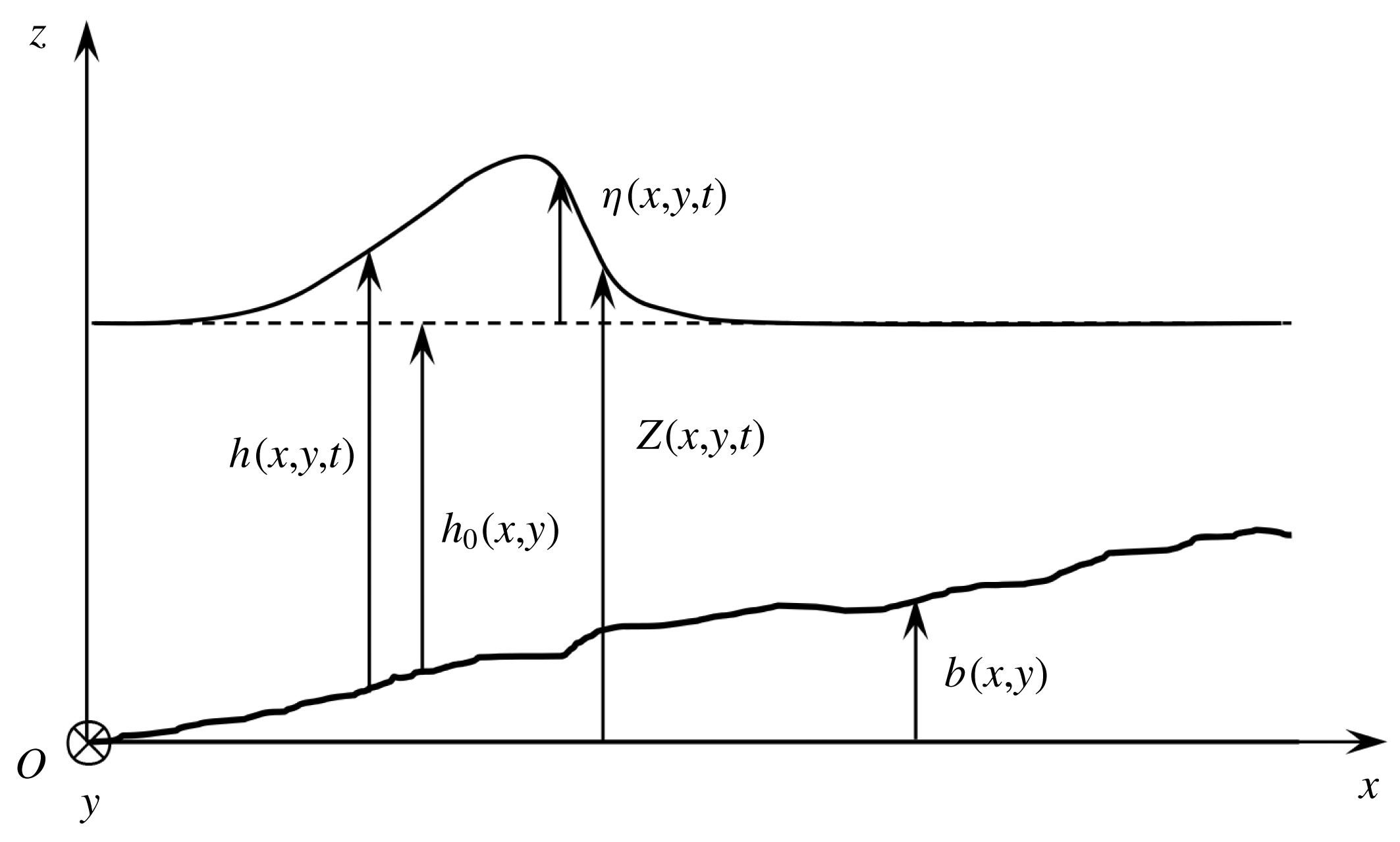
respectively. The water depth is
 $h(x,y,t)=Z(x,y,t)-b(x,y)$
. The still-water depth is
 $h_{0}(x,y)$
and the water elevation is
 $\unicode[STIX]{x1D702}(x,y,t)=h(x,y,t)-h_{0}(x,y)$
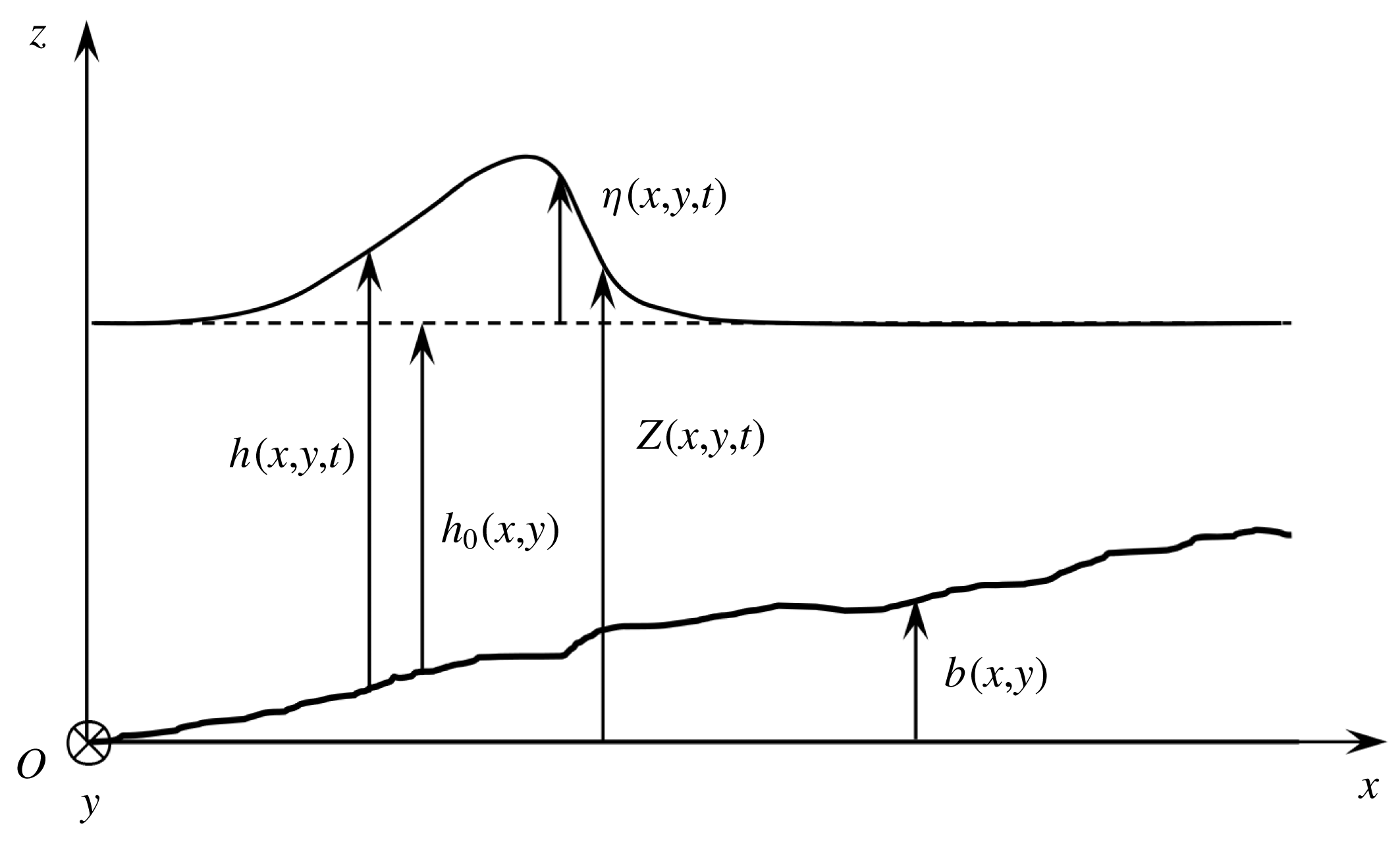
. These notations are depicted in figure 1. It is important to note that the ‘free surface’ referred above is a smooth mean filtered free surface. The boundary conditions for the filtered flow at this mean surface derived by Hasselmann (Reference Hasselmann1971) for non-splashing regimes and by Brocchini & Peregrine (Reference Brocchini and Peregrine2001) for splashing regimes introduce new turbulent stresses at this smooth surface. Although they can have an important role for non-hydrostatic models based on Reynolds-averaged Navier–Stokes equations (Derakhti et al.
Reference Derakhti, Kirby, Shi and Ma2016), they are usually neglected in depth-averaged models. We refer to the Part 1 of this work (Kazakova & Richard Reference Kazakova and Richard2019) for a more complete discussion.
Notations used in the text.
In the following, the operators gradient and divergence are related to a two-dimensional space (
 $Oxy$
) unless noted otherwise. The conventions used for tensor calculus are given in appendix A.
The no-penetration boundary condition at the bottom and the kinematic boundary condition at the free surface can be written respectively
 $$\begin{eqnarray}w(b)=\overline{\boldsymbol{u}}(b)\boldsymbol{\cdot }\mathbf{g}\mathbf{r}\mathbf{a}\mathbf{d}\;b\end{eqnarray}$$
and
 $$\begin{eqnarray}w(Z)=\frac{\unicode[STIX]{x2202}Z}{\unicode[STIX]{x2202}t}+\overline{\boldsymbol{u}}(Z)\boldsymbol{\cdot }\mathbf{g}\mathbf{r}\mathbf{a}\mathbf{d}\;Z.\end{eqnarray}$$
Additionally the dynamic boundary condition at the free surface is
 $(\unicode[STIX]{x1D748}\boldsymbol{\cdot }\boldsymbol{n})(Z)=0$
where
 $\unicode[STIX]{x1D748}$
is the Cauchy stress tensor including the turbulent-viscosity effect and where
 $\boldsymbol{n}$
is the unit normal vector at the free surface. In order to model the shear stress on the bottom wall, the dynamic boundary condition at the bottom can be written
 $(\unicode[STIX]{x1D748}\boldsymbol{\cdot }\boldsymbol{n}^{\prime })(b)=-\hat{p}(b)\boldsymbol{n}^{\prime }-\boldsymbol{f}$
where
 $\boldsymbol{n}^{\prime }$
is the unit normal vector at the bottom,
 $\boldsymbol{f}$
is a friction force to be modelled and
 $\hat{p}$
includes all non-viscous terms i.e. the hydrostatic part of the pressure and all terms due to the dispersive effects and to the variable bottom. The friction force models the shear stress on the bottom and is classically written as a Chézy force or a Manning–Strickler force. This friction term is kept in the derivation of the model but it proved to be useless in the considered applications presented in § 6 and was consequently neglected. This can be explained by the fact that, in the case of breaking waves, the dissipation effects are mainly due to the breaker-generated turbulence rather than to the effects in the bottom boundary layer. The shear stress on the bottom was similarly neglected by Veeramony & Svendsen (Reference Veeramony and Svendsen2000).
2.2 Scaling
According to the shallow-water hypothesis, which is here assumed to be valid, there is a small parameter
 $\unicode[STIX]{x1D707}=h_{0}^{\ast }/L\ll 1$
where
 $h_{0}^{\ast }$
is a reference value of the still-water depth and where
 $L$
is a characteristic length scale in the horizontal plane. A classical scaling is used to write the equations in dimensionless form (see Antuono & Brocchini Reference Antuono and Brocchini2013). The dimensionless quantities are denoted by a tilde symbol and are defined by
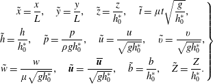 $$\begin{eqnarray}\left.\begin{array}{@{}c@{}}\displaystyle \tilde{x}={\displaystyle \frac{x}{L}},\quad {\tilde{y}}={\displaystyle \frac{y}{L}},\quad \tilde{z}={\displaystyle \frac{z}{h_{0}^{\ast }}},\quad \tilde{t}=\unicode[STIX]{x1D707}t\sqrt{{\displaystyle \frac{g}{h_{0}^{\ast }}}},\\ \displaystyle \tilde{h}={\displaystyle \frac{h}{h_{0}^{\ast }}},\quad \tilde{p}={\displaystyle \frac{p}{\unicode[STIX]{x1D70C}gh_{0}^{\ast }}},\quad \tilde{u} ={\displaystyle \frac{u}{\sqrt{gh_{0}^{\ast }}}},\quad \tilde{v}={\displaystyle \frac{v}{\sqrt{gh_{0}^{\ast }}}},\\ \displaystyle \tilde{w}={\displaystyle \frac{w}{\unicode[STIX]{x1D707}\sqrt{gh_{0}^{\ast }}}},\quad \tilde{\boldsymbol{u}}={\displaystyle \frac{\overline{\boldsymbol{u}}}{\sqrt{gh_{0}^{\ast }}}},\quad \tilde{b}={\displaystyle \frac{b}{h_{0}^{\ast }}},\quad \tilde{Z}={\displaystyle \frac{Z}{h_{0}^{\ast }}}.\end{array}\right\}\end{eqnarray}$$
The viscous stress tensor is defined by
 $\unicode[STIX]{x1D749}=2\unicode[STIX]{x1D70C}\unicode[STIX]{x1D708}\overline{\unicode[STIX]{x1D63F}}=\unicode[STIX]{x1D70F}_{ij}\boldsymbol{e}_{\boldsymbol{i}}\,\otimes \,\boldsymbol{e}_{\boldsymbol{j}}$
where the vectors
 $\boldsymbol{e}_{\boldsymbol{i}}$
are the unit vectors (with Einstein notation and the indexes 1, 2 and 3 for
 $x$
,
 $y$
and
 $z$
respectively). It is scaled as
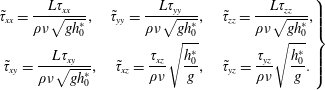 $$\begin{eqnarray}\left.\begin{array}{@{}c@{}}\displaystyle \tilde{\unicode[STIX]{x1D70F}}_{xx}={\displaystyle \frac{L\unicode[STIX]{x1D70F}_{xx}}{\unicode[STIX]{x1D70C}\unicode[STIX]{x1D708}\sqrt{gh_{0}^{\ast }}}},\quad \tilde{\unicode[STIX]{x1D70F}}_{yy}={\displaystyle \frac{L\unicode[STIX]{x1D70F}_{yy}}{\unicode[STIX]{x1D70C}\unicode[STIX]{x1D708}\sqrt{gh_{0}^{\ast }}}},\quad \tilde{\unicode[STIX]{x1D70F}}_{zz}={\displaystyle \frac{L\unicode[STIX]{x1D70F}_{zz}}{\unicode[STIX]{x1D70C}\unicode[STIX]{x1D708}\sqrt{gh_{0}^{\ast }}}},\\ \displaystyle \tilde{\unicode[STIX]{x1D70F}}_{xy}={\displaystyle \frac{L\unicode[STIX]{x1D70F}_{xy}}{\unicode[STIX]{x1D70C}\unicode[STIX]{x1D708}\sqrt{gh_{0}^{\ast }}}},\quad \tilde{\unicode[STIX]{x1D70F}}_{xz}={\displaystyle \frac{\unicode[STIX]{x1D70F}_{xz}}{\unicode[STIX]{x1D70C}\unicode[STIX]{x1D708}}}\sqrt{{\displaystyle \frac{h_{0}^{\ast }}{g}}},\quad \tilde{\unicode[STIX]{x1D70F}}_{yz}={\displaystyle \frac{\unicode[STIX]{x1D70F}_{yz}}{\unicode[STIX]{x1D70C}\unicode[STIX]{x1D708}}}\sqrt{{\displaystyle \frac{h_{0}^{\ast }}{g}}}.\end{array}\right\}\end{eqnarray}$$
It is usual for the modelling of coastal waves to suppose that the Reynolds number defined by
 $Re=h_{0}^{\ast }\sqrt{gh_{0}^{\ast }}/\unicode[STIX]{x1D708}$
is high enough so that the viscous terms are negligible (see for example Antuono & Brocchini Reference Antuono and Brocchini2013). Within the scope of an asymptotic method this hypothesis can be quantified by writing
 $Re=O(\unicode[STIX]{x1D707}^{-4})$
. With the hypothesis of a weakly turbulent flow (see below), this condition reduces to
 $Re=O(\unicode[STIX]{x1D707}^{-3})$
(Kazakova & Richard Reference Kazakova and Richard2019) and this will be assumed in the following.
The ratio
 $\unicode[STIX]{x1D708}_{T}/(h_{0}^{\ast }\sqrt{gh_{0}^{\ast }})$
is typically very small, of the order of
 $10^{-2}$
(Cox, Kobayashi & Okayasu Reference Cox, Kobayashi and Okayasu1995; Svendsen et al.
Reference Svendsen, Veeramony, Bakunin and Kirby2000, see also the discussion in Svendsen Reference Svendsen1987 from various experimental measures). The same scaling as in Antuono & Brocchini (Reference Antuono and Brocchini2013) and in Zhang et al. (Reference Zhang, Kennedy, Donahue, Westerink, Panda and Dawson2014) is used for the eddy viscosity, i.e.
 $$\begin{eqnarray}\tilde{\unicode[STIX]{x1D708}}_{T}=\frac{\unicode[STIX]{x1D708}_{T}}{\unicode[STIX]{x1D707}h_{0}^{\ast }\sqrt{gh_{0}^{\ast }}}.\end{eqnarray}$$
The scaling of the deviatoric part of the residual stress tensor
 $\unicode[STIX]{x1D63C}^{\unicode[STIX]{x1D667}}=2\unicode[STIX]{x1D70C}\unicode[STIX]{x1D708}_{T}\overline{\unicode[STIX]{x1D63F}}=\unicode[STIX]{x1D608}_{ij}^{r}\boldsymbol{e}_{\boldsymbol{i}}\,\otimes \,\boldsymbol{e}_{\boldsymbol{j}}$
is thus
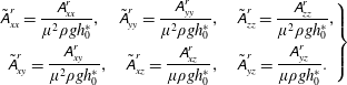 $$\begin{eqnarray}\left.\begin{array}{@{}c@{}}\displaystyle \tilde{\unicode[STIX]{x1D608}}_{xx}^{r}={\displaystyle \frac{\unicode[STIX]{x1D608}_{xx}^{r}}{\unicode[STIX]{x1D707}^{2}\unicode[STIX]{x1D70C}gh_{0}^{\ast }}},\quad \tilde{\unicode[STIX]{x1D608}}_{yy}^{r}={\displaystyle \frac{\unicode[STIX]{x1D608}_{yy}^{r}}{\unicode[STIX]{x1D707}^{2}\unicode[STIX]{x1D70C}gh_{0}^{\ast }}},\quad \tilde{\unicode[STIX]{x1D608}}_{zz}^{r}={\displaystyle \frac{\unicode[STIX]{x1D608}_{zz}^{r}}{\unicode[STIX]{x1D707}^{2}\unicode[STIX]{x1D70C}gh_{0}^{\ast }}},\\ \displaystyle \tilde{\unicode[STIX]{x1D608}}_{xy}^{r}={\displaystyle \frac{\unicode[STIX]{x1D608}_{xy}^{r}}{\unicode[STIX]{x1D707}^{2}\unicode[STIX]{x1D70C}gh_{0}^{\ast }}},\quad \tilde{\unicode[STIX]{x1D608}}_{xz}^{r}={\displaystyle \frac{\unicode[STIX]{x1D608}_{xz}^{r}}{\unicode[STIX]{x1D707}\unicode[STIX]{x1D70C}gh_{0}^{\ast }}},\quad \tilde{\unicode[STIX]{x1D608}}_{yz}^{r}={\displaystyle \frac{\unicode[STIX]{x1D608}_{yz}^{r}}{\unicode[STIX]{x1D707}\unicode[STIX]{x1D70C}gh_{0}^{\ast }}}.\end{array}\right\}\end{eqnarray}$$
It follows that the dimensionless continuity equation writes
 $$\begin{eqnarray}\text{div}\,\tilde{\boldsymbol{u}}+\frac{\unicode[STIX]{x2202}\tilde{w}}{\unicode[STIX]{x2202}\tilde{z}}=0\end{eqnarray}$$
and that the dimensionless momentum equation in the horizontal plane can be written
 $$\begin{eqnarray}\frac{\unicode[STIX]{x2202}\tilde{\boldsymbol{u}}}{\unicode[STIX]{x2202}\tilde{t}}+\mathbf{div}(\tilde{\boldsymbol{u}}\,\otimes \,\tilde{\boldsymbol{u}})+\frac{\unicode[STIX]{x2202}\tilde{w}\tilde{\boldsymbol{u}}}{\unicode[STIX]{x2202}\tilde{z}}+\mathbf{g}\mathbf{r}\mathbf{a}\mathbf{d}\,\tilde{p}=\unicode[STIX]{x1D707}^{2}\mathbf{div}\,\unicode[STIX]{x1D656}+\frac{\unicode[STIX]{x2202}\boldsymbol{a}_{\mathbf{3}}}{\unicode[STIX]{x2202}\tilde{z}}.\end{eqnarray}$$
In this expression, the two-dimensional vector
 $\boldsymbol{a}_{\mathbf{3}}=\tilde{\unicode[STIX]{x1D608}}_{xz}^{r}\boldsymbol{e}_{\boldsymbol{x}}+\tilde{\unicode[STIX]{x1D608}}_{yz}^{r}\boldsymbol{e}_{\boldsymbol{y}}$
is introduced as well as the two-dimensional tensor
 $\unicode[STIX]{x1D656}=2\tilde{\unicode[STIX]{x1D708}}_{T}\unicode[STIX]{x1D668}$
where
 $$\begin{eqnarray}\unicode[STIX]{x1D668}={\textstyle \frac{1}{2}}[\unicode[STIX]{x1D5F4}\unicode[STIX]{x1D5FF}\unicode[STIX]{x1D5EE}\unicode[STIX]{x1D5F1}\,\tilde{\boldsymbol{u}}+(\unicode[STIX]{x1D5F4}\unicode[STIX]{x1D5FF}\unicode[STIX]{x1D5EE}\unicode[STIX]{x1D5F1}\,\tilde{\boldsymbol{u}})^{\text{T}}].\end{eqnarray}$$
We have
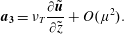 $$\begin{eqnarray}\boldsymbol{a}_{\mathbf{3}}=\unicode[STIX]{x1D708}_{T}\frac{\unicode[STIX]{x2202}\tilde{\boldsymbol{u}}}{\unicode[STIX]{x2202}\tilde{z}}+O(\unicode[STIX]{x1D707}^{2}).\end{eqnarray}$$
The dimensionless momentum equation in the vertical direction
 $Oz$
is
 $$\begin{eqnarray}\unicode[STIX]{x1D707}^{2}\left(\frac{\unicode[STIX]{x2202}\tilde{w}}{\unicode[STIX]{x2202}\tilde{t}}+\frac{\unicode[STIX]{x2202}\tilde{u} \tilde{w}}{\unicode[STIX]{x2202}\tilde{x}}+\frac{\unicode[STIX]{x2202}\tilde{v}\tilde{w}}{\unicode[STIX]{x2202}{\tilde{y}}}+\frac{\unicode[STIX]{x2202}\tilde{w}^{2}}{\unicode[STIX]{x2202}\tilde{z}}\right)=-1-\frac{\unicode[STIX]{x2202}\tilde{p}}{\unicode[STIX]{x2202}\tilde{z}}+\unicode[STIX]{x1D707}^{2}\frac{\tilde{\unicode[STIX]{x1D608}}_{xz}^{r}}{\unicode[STIX]{x2202}\tilde{x}}+\unicode[STIX]{x1D707}^{2}\frac{\tilde{\unicode[STIX]{x1D608}}_{yz}^{r}}{\unicode[STIX]{x2202}{\tilde{y}}}+\unicode[STIX]{x1D707}^{2}\frac{\tilde{\unicode[STIX]{x1D608}}_{zz}^{r}}{\unicode[STIX]{x2202}\tilde{z}}.\end{eqnarray}$$
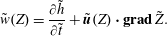
The no-penetration boundary condition writes
 $\tilde{w}(b)=\tilde{\boldsymbol{u}}(b)\boldsymbol{\cdot }\mathbf{g}\mathbf{r}\mathbf{a}\mathbf{d}\,\tilde{b}$
while the kinematic boundary condition is
 $$\begin{eqnarray}\tilde{w}(Z)=\frac{\unicode[STIX]{x2202}\tilde{h}}{\unicode[STIX]{x2202}\tilde{t}}+\tilde{\boldsymbol{u}}(Z)\boldsymbol{\cdot }\mathbf{g}\mathbf{r}\mathbf{a}\mathbf{d}\,\tilde{Z}.\end{eqnarray}$$
The dynamic boundary condition at the free surface becomes in dimensionless form
 $$\begin{eqnarray}\displaystyle & \displaystyle \boldsymbol{a}_{\mathbf{3}}(Z)+\tilde{p}(Z)\mathbf{g}\mathbf{r}\mathbf{a}\mathbf{d}\,\tilde{Z}-\unicode[STIX]{x1D707}^{2}\unicode[STIX]{x1D656}(Z)\boldsymbol{\cdot }\mathbf{g}\mathbf{r}\mathbf{a}\mathbf{d}\,Z=0, & \displaystyle\end{eqnarray}$$
 $$\begin{eqnarray}\displaystyle & \displaystyle \tilde{p}(Z)+\unicode[STIX]{x1D707}^{2}\boldsymbol{a}_{\mathbf{3}}(Z)\boldsymbol{\cdot }\mathbf{g}\mathbf{r}\mathbf{a}\mathbf{d}\,\tilde{Z}-\unicode[STIX]{x1D707}^{2}\tilde{\unicode[STIX]{x1D608}}_{zz}^{r}(Z)=0. & \displaystyle\end{eqnarray}$$
All capillary effects are neglected. The dynamic boundary conditions on the bottom write
 $$\begin{eqnarray}\displaystyle & \displaystyle \boldsymbol{a}_{\mathbf{3}}(b)+\tilde{p}(b)\mathbf{g}\mathbf{r}\mathbf{a}\mathbf{d}\,\tilde{b}-\unicode[STIX]{x1D707}^{2}\unicode[STIX]{x1D656}(b)\boldsymbol{\cdot }\mathbf{g}\mathbf{r}\mathbf{a}\mathbf{d}\,b=\hat{p}(b)\mathbf{g}\mathbf{r}\mathbf{a}\mathbf{d}\,\tilde{b}-\unicode[STIX]{x1D707}^{2}\boldsymbol{f}, & \displaystyle\end{eqnarray}$$
 $$\begin{eqnarray}\displaystyle & \displaystyle \tilde{p}(b)+\unicode[STIX]{x1D707}^{2}\boldsymbol{a}_{\mathbf{3}}(b)\boldsymbol{\cdot }\mathbf{g}\mathbf{r}\mathbf{a}\mathbf{d}\,\tilde{b}-\unicode[STIX]{x1D707}^{2}\tilde{\unicode[STIX]{x1D608}}_{zz}^{r}(b)=\hat{p}(b). & \displaystyle\end{eqnarray}$$
The friction force on the bottom is supposed to be of
 $O(\unicode[STIX]{x1D707}^{2})$
. In these expressions,
 $\hat{p}$
and
 $f$
denote dimensionless quantities.
2.3 Averaged mass and momentum equations
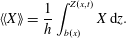
The equations (2.11), (2.12) and (2.15) are averaged over the depth taking into account the boundary conditions. The averaged quantity corresponding to any quantity
 $X$
is defined as
 $$\begin{eqnarray}\langle \langle X\rangle \rangle =\frac{1}{h}\int _{b(x)}^{Z(x,t)}X\,\text{d}z.\end{eqnarray}$$
The two-dimensional average velocity vector is denoted by
 $\boldsymbol{U}=\langle \langle \overline{\boldsymbol{u}}\rangle \rangle$
and its components in the
 $Ox$
and
 $Oy$
directions are denoted by
 $U$
and
 $V$
respectively. The filtered horizontal velocity vector is decomposed as the sum of its averaged value and of a deviation
 $\boldsymbol{u}^{\prime }$
representing the large-scale turbulence and the shearing effects i.e.
 $$\begin{eqnarray}\overline{\boldsymbol{u}}(x,y,z,t)=\boldsymbol{U}(x,y,t)+\boldsymbol{u}^{\prime }(x,y,z,t).\end{eqnarray}$$
In the same way as in Teshukov (Reference Teshukov2007), the flow is supposed to be weakly turbulent (see Kazakova & Richard Reference Kazakova and Richard2019). This means that
 $\boldsymbol{u}^{\prime }=O(\unicode[STIX]{x1D707})$
and that in dimensionless form
 $\tilde{\boldsymbol{u}}=\tilde{\boldsymbol{U}}+\unicode[STIX]{x1D707}\tilde{\boldsymbol{u}}^{\prime }$
. The same hypothesis was used by Castro & Lannes (Reference Castro and Lannes2014).
This assumption is equivalent to the underlying hypotheses in other models. In eddy-viscosity models for instance, the turbulent viscosity is of
 $O(\unicode[STIX]{x1D707})$
in accordance with experimental results as explained above. Since the eddy viscosity can be written
 $\unicode[STIX]{x1D708}_{T}=c\,\ell _{m}\sqrt{k}$
, where
 $c$
is a dimensionless constant of
 $O(1)$
and
 $\ell _{m}$
a mixing length of
 $O(h)$
, the turbulent kinetic energy is of
 $O(\unicode[STIX]{x1D707}^{2})$
. This is exactly the same order of magnitude as the turbulent energy that is obtained with the weak turbulence assumption. In the switching models or in the nonlinear shallow-water models (Saint-Venant equations) the turbulence is not modelled at all (apart from drag forces which model effects at the bottom boundary layer) which does not prevent these models from having been successfully applied to breaking waves. In this case the turbulent dissipation is handled by the discontinuities produced by these hyperbolic equations and this implies that the front parts of breaking waves cannot be correctly described since they reduce to shock waves. The same problem is found with turbulent hydraulic jumps which are treated as discontinuities in the Saint-Venant system. This problem was improved within the scope of a new hyperbolic system based on the weak turbulence (or weak shear) assumption by Richard & Gavrilyuk (Reference Richard and Gavrilyuk2013) who were able to model correctly strong hydraulic jumps with an upstream Froude number as high as 16 and consequently with a very strong turbulence. It follows that, in spite of its name, the assumption of weakly turbulent flows does not prevent the application of the model to breaking waves in the surf zone and is an improvement on the switching models which are commonly used for these waves.
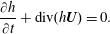
In the following the tilde symbols for dimensionless quantities are dropped to lighten the notations. After averaging over the depth, the mass equation becomes
 $$\begin{eqnarray}\frac{\unicode[STIX]{x2202}h}{\unicode[STIX]{x2202}t}+\text{div}(h\boldsymbol{U})=0.\end{eqnarray}$$
With the kinematic boundary condition at the free surface, the averaging over the depth of the three first terms of the momentum equation (2.12) yields
 $$\begin{eqnarray}\int _{b}^{Z}\left[\frac{\unicode[STIX]{x2202}\boldsymbol{u}}{\unicode[STIX]{x2202}t}+\mathbf{div}(\boldsymbol{u}\,\otimes \,\boldsymbol{u})+\frac{\unicode[STIX]{x2202}w\boldsymbol{u}}{\unicode[STIX]{x2202}z}\right]\,\text{d}z=\frac{\unicode[STIX]{x2202}h\boldsymbol{U}}{\unicode[STIX]{x2202}t}+\mathbf{div}\int _{b}^{Z}\boldsymbol{u}\,\otimes \,\boldsymbol{u}\,\text{d}z.\end{eqnarray}$$
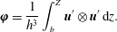
The approach of Teshukov (Reference Teshukov2007) is followed here for the treatment of the integral of
 $\boldsymbol{u}\,\otimes \,\boldsymbol{u}$
. The enstrophy tensor is defined as
 $$\begin{eqnarray}\unicode[STIX]{x1D753}=\frac{1}{h^{3}}\int _{b}^{Z}\boldsymbol{u}^{\prime }\,\otimes \,\boldsymbol{u}^{\prime }\,\text{d}z.\end{eqnarray}$$
Since, by definition,
 $\langle \langle \boldsymbol{u}^{\prime }\rangle \rangle =0$
, we can write
 $\langle \langle \boldsymbol{u}\,\otimes \,\boldsymbol{u}\rangle \rangle =\boldsymbol{U}\,\otimes \,\boldsymbol{U}+\unicode[STIX]{x1D707}^{2}h^{2}\unicode[STIX]{x1D753}$
. This gives
 $$\begin{eqnarray}\int _{b}^{Z}\left[\frac{\unicode[STIX]{x2202}\boldsymbol{u}}{\unicode[STIX]{x2202}t}+\mathbf{div}(\boldsymbol{u}\,\otimes \,\boldsymbol{u})+\frac{\unicode[STIX]{x2202}w\boldsymbol{u}}{\unicode[STIX]{x2202}z}\right]\,\text{d}z=\frac{\unicode[STIX]{x2202}h\boldsymbol{U}}{\unicode[STIX]{x2202}t}+\mathbf{div}(h\boldsymbol{U}\,\otimes \,\boldsymbol{U}+\unicode[STIX]{x1D707}^{2}h^{3}\unicode[STIX]{x1D753}).\end{eqnarray}$$
The equation (2.15) is needed to calculate the pressure term. First the material derivative of
 $h$
is defined as
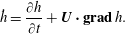 $$\begin{eqnarray}{\dot{h}}=\frac{\unicode[STIX]{x2202}h}{\unicode[STIX]{x2202}t}+\boldsymbol{U}\boldsymbol{\cdot }\mathbf{g}\mathbf{r}\mathbf{a}\mathbf{d}\,h.\end{eqnarray}$$
Second an expression of the vertical velocity
 $w$
can be obtained from the continuity equation. We get
 $$\begin{eqnarray}w=(z-b)\frac{{\dot{h}}}{h}+\boldsymbol{U}\boldsymbol{\cdot }\mathbf{g}\mathbf{r}\mathbf{a}\mathbf{d}\,b+O(\unicode[STIX]{x1D707}).\end{eqnarray}$$
Then the left-hand part of (2.15) can be written
 $$\begin{eqnarray}\frac{\unicode[STIX]{x2202}w}{\unicode[STIX]{x2202}t}+\frac{\unicode[STIX]{x2202}uw}{\unicode[STIX]{x2202}x}+\frac{\unicode[STIX]{x2202}vw}{\unicode[STIX]{x2202}y}+\frac{\unicode[STIX]{x2202}w^{2}}{\unicode[STIX]{x2202}z}=(z-b)\frac{\ddot{h}}{h}+\frac{\text{D}}{\text{D}t}(\boldsymbol{U}\boldsymbol{\cdot }\mathbf{g}\mathbf{r}\mathbf{a}\mathbf{d}\,b)+O(\unicode[STIX]{x1D707}),\end{eqnarray}$$
where the material derivative has the same meaning as the dot in (2.27) i.e.
 $\text{D}X/\text{D}t=\unicode[STIX]{x2202}X/\unicode[STIX]{x2202}t+\boldsymbol{U}\boldsymbol{\cdot }\mathbf{g}\mathbf{r}\mathbf{a}\mathbf{d}\,X$
for any scalar quantity
 $X$
. We denote by
 $\ddot{h}$
the material derivative of
 ${\dot{h}}$
along the average flow i.e.
 $$\begin{eqnarray}\displaystyle \ddot{h} & = & \displaystyle {\displaystyle \frac{\unicode[STIX]{x2202}{\dot{h}}}{\unicode[STIX]{x2202}t}}+U{\displaystyle \frac{\unicode[STIX]{x2202}{\dot{h}}}{\unicode[STIX]{x2202}x}}\end{eqnarray}$$
 $$\begin{eqnarray}\displaystyle & = & \displaystyle h\left({\displaystyle \frac{\unicode[STIX]{x2202}U}{\unicode[STIX]{x2202}x}}\right)^{2}-h{\displaystyle \frac{\unicode[STIX]{x2202}^{2}U}{\unicode[STIX]{x2202}x\unicode[STIX]{x2202}t}}-hU{\displaystyle \frac{\unicode[STIX]{x2202}^{2}U}{\unicode[STIX]{x2202}x^{2}}}.\end{eqnarray}$$
The term in
 $\ddot{h}$
is a source of difficulties for the numerical resolution and a special treatment is needed to handle it properly (see § 4).
This result is used to calculate the part of the pressure term that does not depend on the eddy viscosity. Using the boundary conditions, we find
 $$\begin{eqnarray}\int _{b}^{Z}p\,\text{d}z=\frac{h^{2}}{2}+\unicode[STIX]{x1D707}^{2}\frac{h^{2}\ddot{h}}{3}+\unicode[STIX]{x1D707}^{2}\frac{h^{2}}{2}\frac{\text{D}}{\text{D}t}(\boldsymbol{U}\boldsymbol{\cdot }\mathbf{g}\mathbf{r}\mathbf{a}\mathbf{d}\,b)+\unicode[STIX]{x1D707}^{2}F_{1},\end{eqnarray}$$
where
 $F_{1}$
is the integral of viscous terms
 $$\begin{eqnarray}F_{1}=\int _{b}^{Z}\text{d}z\frac{\unicode[STIX]{x2202}}{\unicode[STIX]{x2202}x}\int _{Z}^{z}\unicode[STIX]{x1D608}_{xz}^{r}\,\text{d}z+\int _{b}^{Z}\text{d}z\frac{\unicode[STIX]{x2202}}{\unicode[STIX]{x2202}y}\int _{Z}^{z}\unicode[STIX]{x1D608}_{yz}^{r}\,\text{d}z+\int _{b}^{Z}\unicode[STIX]{x1D608}_{zz}^{r}\,\text{d}z.\end{eqnarray}$$
As in Part 1 of this work (Kazakova & Richard Reference Kazakova and Richard2019), the turbulent viscosity is assumed to be uniform over the depth. A depth-uniform eddy viscosity was also assumed by Zhang et al. (Reference Zhang, Kennedy, Donahue, Westerink, Panda and Dawson2014). This hypothesis is sufficient for the applications to coastal wave modelling. A depth-variable eddy viscosity would increase considerably the complexity of the model for little benefit. It follows from this assumption and from the hypothesis of a weakly turbulent flow that
 $$\begin{eqnarray}\int _{b}^{Z}\text{d}z\frac{\unicode[STIX]{x2202}}{\unicode[STIX]{x2202}x}\int _{Z}^{z}\unicode[STIX]{x1D608}_{xz}^{r}\,\text{d}z=O(\unicode[STIX]{x1D707})\quad \text{and}\quad \int _{b}^{Z}\text{d}z\frac{\unicode[STIX]{x2202}}{\unicode[STIX]{x2202}y}\int _{Z}^{z}\unicode[STIX]{x1D608}_{yz}^{r}\,\text{d}z=O(\unicode[STIX]{x1D707}).\end{eqnarray}$$
These two integrals can therefore be neglected. In the same way, we get
 $\boldsymbol{a}_{\mathbf{3}}=O(\unicode[STIX]{x1D707})$
. It follows that the dynamic boundary conditions on the bottom yield
 $$\begin{eqnarray}\boldsymbol{a}_{\mathbf{3}}(b)+\unicode[STIX]{x1D707}^{2}\unicode[STIX]{x1D608}_{zz}^{r}(b)\mathbf{g}\mathbf{r}\mathbf{a}\mathbf{d}\,b-\unicode[STIX]{x1D707}^{2}\unicode[STIX]{x1D656}(b)\boldsymbol{\cdot }\mathbf{g}\mathbf{r}\mathbf{a}\mathbf{d}\,b=-\unicode[STIX]{x1D707}^{2}\boldsymbol{f}.\end{eqnarray}$$
Using again the boundary conditions, this leads to the following expression for the averaged momentum balance equation
 $$\begin{eqnarray}\displaystyle & & \displaystyle \frac{\unicode[STIX]{x2202}h\boldsymbol{U}}{\unicode[STIX]{x2202}t}+\mathbf{div}(h\boldsymbol{U}\,\otimes \,\boldsymbol{U}+\unicode[STIX]{x1D707}^{2}h^{3}\unicode[STIX]{x1D753})+\mathbf{g}\mathbf{r}\mathbf{a}\mathbf{d}\left(\frac{h^{2}}{2}+\unicode[STIX]{x1D707}^{2}\frac{h^{2}\ddot{h}}{3}+\unicode[STIX]{x1D707}^{2}\unicode[STIX]{x1D6F1}^{\prime }\right)\nonumber\\ \displaystyle & & \displaystyle \quad =-\hat{p}(b)\mathbf{g}\mathbf{r}\mathbf{a}\mathbf{d}\,b+\unicode[STIX]{x1D707}^{2}\boldsymbol{f}+\unicode[STIX]{x1D707}^{2}\mathbf{div}\int _{b}^{Z}\unicode[STIX]{x1D656}\,\text{d}z-\unicode[STIX]{x1D707}^{2}\mathbf{g}\mathbf{r}\mathbf{a}\mathbf{d}\int _{b}^{Z}\unicode[STIX]{x1D608}_{zz}^{r}\,\text{d}z+O(\unicode[STIX]{x1D707}^{3}),\qquad\end{eqnarray}$$
where
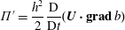 $$\begin{eqnarray}\unicode[STIX]{x1D6F1}^{\prime }=\frac{h^{2}}{2}\frac{\text{D}}{\text{D}t}(\boldsymbol{U}\boldsymbol{\cdot }\mathbf{g}\mathbf{r}\mathbf{a}\mathbf{d}\,b)\end{eqnarray}$$
and
 $\hat{p}(b)=h+\unicode[STIX]{x1D707}^{2}h\ddot{h}/2+\unicode[STIX]{x1D707}^{2}2\unicode[STIX]{x1D6F1}^{\prime }/h+O(\unicode[STIX]{x1D707}^{3})$
is the pressure on the bottom to the exclusion of all viscous effects. All viscous effects at the bottom are modelled by the friction force
 $\boldsymbol{f}$
. The continuity equation implies that
 $\unicode[STIX]{x1D608}_{zz}^{r}=-\unicode[STIX]{x1D608}_{xx}^{r}-\unicode[STIX]{x1D608}_{yy}^{r}$
. The calculation of the last integrals leads to
 $$\begin{eqnarray}\displaystyle & & \displaystyle \frac{\unicode[STIX]{x2202}h\boldsymbol{U}}{\unicode[STIX]{x2202}t}+\mathbf{div}(h\boldsymbol{U}\,\otimes \,\boldsymbol{U}+\unicode[STIX]{x1D707}^{2}h^{3}\unicode[STIX]{x1D753})+\mathbf{g}\mathbf{r}\mathbf{a}\mathbf{d}\left(\frac{h^{2}}{2}+\unicode[STIX]{x1D707}^{2}\frac{h^{2}\ddot{h}}{3}+\unicode[STIX]{x1D707}^{2}\unicode[STIX]{x1D6F1}^{\prime }\right)\nonumber\\ \displaystyle & & \displaystyle \quad =-h\,\mathbf{g}\mathbf{r}\mathbf{a}\mathbf{d}\,b+\unicode[STIX]{x1D707}^{2}\mathbf{div}(h\unicode[STIX]{x1D63C})+\unicode[STIX]{x1D707}^{2}(\boldsymbol{f}-\boldsymbol{f}^{\prime })+O(\unicode[STIX]{x1D707}^{3}).\end{eqnarray}$$
The expression of the quantity
 $\boldsymbol{f}^{\prime }$
is
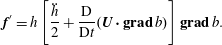 $$\begin{eqnarray}\boldsymbol{f}^{\prime }=h\left[\frac{\ddot{h}}{2}+\frac{\text{D}}{\text{D}t}(\boldsymbol{U}\boldsymbol{\cdot }\mathbf{g}\mathbf{r}\mathbf{a}\mathbf{d}\,b)\right]\mathbf{g}\mathbf{r}\mathbf{a}\mathbf{d}\,b.\end{eqnarray}$$
It encompasses terms due to the variable bottom of
 $O(\unicode[STIX]{x1D707}^{2})$
. The tensor
 $\unicode[STIX]{x1D63C}$
satisfies the relation
 $$\begin{eqnarray}\unicode[STIX]{x1D63C}=2\unicode[STIX]{x1D708}_{T}\unicode[STIX]{x1D64E}+2\unicode[STIX]{x1D708}_{T}(\text{div}\,\boldsymbol{U})\unicode[STIX]{x1D644},\end{eqnarray}$$
where
 $\unicode[STIX]{x1D644}$
is the identity tensor (two-dimensional) and where
 $$\begin{eqnarray}\unicode[STIX]{x1D64E}={\textstyle \frac{1}{2}}[\unicode[STIX]{x1D5F4}\unicode[STIX]{x1D5FF}\unicode[STIX]{x1D5EE}\unicode[STIX]{x1D5F1}\,\boldsymbol{U}+(\unicode[STIX]{x1D5F4}\unicode[STIX]{x1D5FF}\unicode[STIX]{x1D5EE}\unicode[STIX]{x1D5F1}\,\boldsymbol{U})^{\text{T}}].\end{eqnarray}$$
This tensor
 $\unicode[STIX]{x1D63C}$
acts like the viscous stress tensor of a compressible fluid. The averaged mass equation (2.23) of the model is analogous to the mass conservation equation of a compressible fluid, the depth
 $h$
being analogous to the density. The relation (2.40) is then analogous to the constitutive equation of a Newtonian compressible fluid i.e.
 $\unicode[STIX]{x1D749}=2\unicode[STIX]{x1D707}\unicode[STIX]{x1D63F}+\unicode[STIX]{x1D702}(\text{div}\,\boldsymbol{v})\unicode[STIX]{x1D644}_{\unicode[STIX]{x1D7EF}}$
where
 $\unicode[STIX]{x1D63F}$
is the strain rate tensor,
 $\unicode[STIX]{x1D644}_{\unicode[STIX]{x1D7EF}}$
the three-dimensional identity tensor,
 $\boldsymbol{v}$
is the velocity field (the operator divergence is here three-dimensional),
 $\unicode[STIX]{x1D707}$
and
 $\unicode[STIX]{x1D702}$
being the first and second viscosities respectively. In the case of the model, the first viscosity is equal to the turbulent viscosity
 $\unicode[STIX]{x1D708}_{T}$
and the second viscosity is equal to
 $2\unicode[STIX]{x1D708}_{T}$
. Note that
 $\unicode[STIX]{x1D64E}$
is not a deviator since
 $\text{tr}\,\unicode[STIX]{x1D64E}=\text{div}\,\boldsymbol{U}\neq 0$
. For compressible fluids, it is more convenient to define the deviatoric tensor
 $\unicode[STIX]{x1D64E}_{\unicode[STIX]{x1D7EC}}=\unicode[STIX]{x1D64E}-(\text{div}\,\boldsymbol{U})\unicode[STIX]{x1D644}/2$
(this gives
 $\text{tr}\,\unicode[STIX]{x1D64E}_{\unicode[STIX]{x1D7EC}}=0$
since
 $\text{tr}\,\unicode[STIX]{x1D644}=2$
in a two-dimensional space). The tensor
 $\unicode[STIX]{x1D63C}$
can then be written
 $$\begin{eqnarray}\unicode[STIX]{x1D63C}=2\unicode[STIX]{x1D708}_{T}\unicode[STIX]{x1D64E}_{\unicode[STIX]{x1D7EC}}+\unicode[STIX]{x1D701}(\text{div}\,\boldsymbol{U})\unicode[STIX]{x1D644},\end{eqnarray}$$
where
 $\unicode[STIX]{x1D701}=3\unicode[STIX]{x1D708}_{T}$
is the sum of the first and second viscosities and is the volume viscosity of the model (in a three-dimensional space, the volume viscosity is equal to
 $\unicode[STIX]{x1D702}+2\unicode[STIX]{x1D707}/3$
). The first viscosity and the volume viscosity are both positive, which is in accordance with the second law of thermodynamics. Note that the Stokes hypothesis, according to which the volume viscosity is equal to zero, is not satisfied in the model.
The gradient term on the left-hand side of (2.38) includes dispersive effects originating from a non-hydrostatic correction to the pressure. It should be noted that no smallness assumption was made on the nonlinearity, which implies that the model is fully nonlinear. Its dispersive properties are identical to those of the Green–Naghdi equations. An improvement of these properties is proposed in § 4.
The model is anisotropic due to the anisotropy of the symmetrical enstrophy tensor
 $\unicode[STIX]{x1D753}$
. The definition (2.25) of the enstrophy tensor shows clearly that
 $\unicode[STIX]{x1D753}$
is symmetrical. However it is not an isotropic tensor since its deviatoric part
 $\unicode[STIX]{x1D753}^{D}=\unicode[STIX]{x1D753}-\text{tr}\unicode[STIX]{x1D753}\,\unicode[STIX]{x1D644}/2$
is not zero. The tensor
 $\unicode[STIX]{x1D753}$
has three independent components denoted by
 $\unicode[STIX]{x1D711}_{11}$
,
 $\unicode[STIX]{x1D711}_{12}$
and
 $\unicode[STIX]{x1D711}_{22}$
which are defined by
 $\unicode[STIX]{x1D753}=\unicode[STIX]{x1D711}_{11}\boldsymbol{e}_{\boldsymbol{x}}\,\otimes \,\boldsymbol{e}_{\boldsymbol{x}}+\unicode[STIX]{x1D711}_{12}\boldsymbol{e}_{\boldsymbol{x}}\,\otimes \,\boldsymbol{e}_{\boldsymbol{y}}+\unicode[STIX]{x1D711}_{12}\boldsymbol{e}_{\boldsymbol{y}}\,\otimes \,\boldsymbol{e}_{\boldsymbol{x}}+\unicode[STIX]{x1D711}_{22}\boldsymbol{e}_{\boldsymbol{y}}\,\otimes \,\boldsymbol{e}_{\boldsymbol{y}}$
. This tensor represents the large-scale turbulence and the shearing effects. The large-scale turbulence of the energy-containing range has an anisotropic character which is thus taken into account in the model through the anisotropic tensor
 $\unicode[STIX]{x1D753}$
.
This is one of the main advantages of this approach in comparison with the classical approaches modelling all turbulence with an eddy viscosity. A viscosity hypothesis is a valid model for turbulence if this one is reasonably isotropic and not too far from the equilibrium between production and dissipation. These two conditions are questionable in the case of the turbulence of a breaking wave. Consequently the classical eddy-viscosity approaches for breaking waves misses the anisotropic effects of the large-scale turbulence (Nadaoka & Yagi Reference Nadaoka and Yagi1998). Furthermore, there is no backscatter with an eddy-viscosity model and consequently no energy transfer from the horizontal three-dimensional eddies towards the vertical two-dimensional eddies and yet this transfer can happen (see for example Nadaoka & Yagi Reference Nadaoka and Yagi1998; Hinterberger et al. Reference Hinterberger, Fröhlich and Rodi2007).
With our depth-averaged large-eddy simulation (LES) approach with a cutoff frequency in the inertial subrange, only the small-scale turbulence is modelled by a turbulent-viscosity hypothesis while the anisotropic large-scale turbulence of the energy-containing range is resolved. Both the isotropic and equilibrium conditions are well satisfied for the small-scale turbulence (see for example Kolmogorov’s hypotheses, Kolmogorov Reference Kolmogorov1941) and the absence of backscatter from the small scales towards the large scales is a very classical view in accordance with the energy cascade of Richardson (Reference Richardson1922) which was confirmed experimentally in the case of breaking waves by Hattori & Aono (Reference Hattori and Aono1985). The introduction of the eddy viscosity has thus better physical justifications than for the classical eddy-viscosity models. The anisotropic character of our equations has a physical basis and on the whole the resolution of the large-scale turbulence gives our model a richer physical content.
The model features six scalar unknowns which are the water depth
 $h$
, the components
 $U$
and
 $V$
of the average velocity field in the
 $Ox$
and
 $Oy$
directions respectively and the three components of the enstrophy tensor. The mass (2.23) and momentum (2.38) equations provide three scalar equations. Three more equations are thus needed to close the system. In the one-dimensional case (Kazakova & Richard Reference Kazakova and Richard2019) the closure was obtained with the energy equation. In this two-dimensional case, the energy equation gives only one scalar equation and it is not sufficient. In the one-dimensional (1-D) case the energy equation could be replaced with the enstrophy equation which was one scalar equation since the 1-D enstrophy is a scalar. In the two-dimensional (2-D) case the enstrophy tensor equation is used to provide the three remaining scalar equations.
2.4 Enstrophy tensor equation
The tilde symbols are also dropped in this section. The first step to derive the enstrophy tensor equation is to form the tensor product u ⊗ (2.12) + (2.12) ⊗ u . Taking into account the boundary conditions, this leads to
 $$\begin{eqnarray}\displaystyle & & \displaystyle \frac{\unicode[STIX]{x2202}\boldsymbol{u}\,\otimes \,\boldsymbol{u}}{\unicode[STIX]{x2202}t}+\unicode[STIX]{x1D5F1}\unicode[STIX]{x1D5F6}\unicode[STIX]{x1D603}(\boldsymbol{u}\,\otimes \,\boldsymbol{u}\,\otimes \,\boldsymbol{u})+\frac{\unicode[STIX]{x2202}}{\unicode[STIX]{x2202}z}(w\boldsymbol{u}\,\otimes \,\boldsymbol{u})+\boldsymbol{u}\,\otimes \,\mathbf{g}\mathbf{r}\mathbf{a}\mathbf{d}\,p+\mathbf{g}\mathbf{r}\mathbf{a}\mathbf{d}\,p\,\otimes \,\boldsymbol{u}\nonumber\\ \displaystyle & & \displaystyle \quad =\unicode[STIX]{x1D707}^{2}\boldsymbol{u}\,\otimes \,\mathbf{div}\,\unicode[STIX]{x1D656}+\unicode[STIX]{x1D707}^{2}\mathbf{div}\,\unicode[STIX]{x1D656}\,\otimes \,\boldsymbol{u}+\unicode[STIX]{x1D708}_{T}\boldsymbol{u}\,\otimes \,\frac{\unicode[STIX]{x2202}^{2}\boldsymbol{u}}{\unicode[STIX]{x2202}z^{2}}+\unicode[STIX]{x1D708}_{T}\frac{\unicode[STIX]{x2202}^{2}\boldsymbol{u}}{\unicode[STIX]{x2202}z^{2}}\,\otimes \,\boldsymbol{u}.\end{eqnarray}$$
The second step is to average this equation over the depth, again with the boundary conditions. This procedure yields
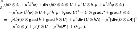 $$\begin{eqnarray}\displaystyle & & \displaystyle \frac{\unicode[STIX]{x2202}}{\unicode[STIX]{x2202}t}(h\boldsymbol{U}\,\otimes \,\boldsymbol{U}+\unicode[STIX]{x1D707}^{2}h^{3}\unicode[STIX]{x1D753})+\unicode[STIX]{x1D5F1}\unicode[STIX]{x1D5F6}\unicode[STIX]{x1D603}\,(h\boldsymbol{U}\,\otimes \,\boldsymbol{U}\,\otimes \,\boldsymbol{U}+\unicode[STIX]{x1D707}^{2}\boldsymbol{U}\,\otimes \,h^{3}\unicode[STIX]{x1D753}+\unicode[STIX]{x1D707}^{2}h^{3}\unicode[STIX]{x1D753}\,\otimes \,\boldsymbol{U})\nonumber\\ \displaystyle & & \displaystyle \qquad +\,\unicode[STIX]{x1D707}^{2}\mathbf{div}\,(h^{3}\unicode[STIX]{x1D753})\,\otimes \,\boldsymbol{U}+\unicode[STIX]{x1D707}^{2}h^{3}\unicode[STIX]{x1D753}\boldsymbol{\cdot }(\unicode[STIX]{x1D5F4}\unicode[STIX]{x1D5FF}\unicode[STIX]{x1D5EE}\unicode[STIX]{x1D5F1}\,\boldsymbol{U})^{\text{T}}+\boldsymbol{U}\,\otimes \,\mathbf{g}\mathbf{r}\mathbf{a}\mathbf{d}\,P+\mathbf{g}\mathbf{r}\mathbf{a}\mathbf{d}\,P\,\otimes \,\boldsymbol{U}\nonumber\\ \displaystyle & & \displaystyle \quad =-\hat{p}(b)(\boldsymbol{U}\,\otimes \,\mathbf{g}\mathbf{r}\mathbf{a}\mathbf{d}\,b+\mathbf{g}\mathbf{r}\mathbf{a}\mathbf{d}\,b\,\otimes \,\boldsymbol{U})+\unicode[STIX]{x1D707}^{2}\unicode[STIX]{x1D5F1}\unicode[STIX]{x1D5F6}\unicode[STIX]{x1D603}\,(\boldsymbol{U}\,\otimes \,h\unicode[STIX]{x1D63C})+\unicode[STIX]{x1D707}^{2}[\unicode[STIX]{x1D5F1}\unicode[STIX]{x1D5F6}\unicode[STIX]{x1D603}(\boldsymbol{U}\,\otimes \,h\unicode[STIX]{x1D63C})]^{\text{T}}\nonumber\\ \displaystyle & & \displaystyle \qquad +\,\unicode[STIX]{x1D707}^{2}\boldsymbol{U}\,\otimes \,\,\boldsymbol{f}+\unicode[STIX]{x1D707}^{2}\boldsymbol{f}\,\otimes \,\boldsymbol{U}-\unicode[STIX]{x1D707}^{2}h\langle \langle \unicode[STIX]{x1D64B}^{\unicode[STIX]{x1D667}}\rangle \rangle +O(\unicode[STIX]{x1D707}^{3}),\end{eqnarray}$$
where
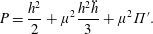 $$\begin{eqnarray}P=\frac{h^{2}}{2}+\unicode[STIX]{x1D707}^{2}\frac{h^{2}\ddot{h}}{3}+\unicode[STIX]{x1D707}^{2}\unicode[STIX]{x1D6F1}^{\prime }.\end{eqnarray}$$
The tensor
 $\unicode[STIX]{x1D64B}^{\unicode[STIX]{x1D667}}$
includes all dissipative effects and its expression is
 $$\begin{eqnarray}\unicode[STIX]{x1D64B}^{\unicode[STIX]{x1D667}}=\unicode[STIX]{x1D5F4}\unicode[STIX]{x1D5FF}\unicode[STIX]{x1D5EE}\unicode[STIX]{x1D5F1}\,\boldsymbol{u}\boldsymbol{\cdot }\unicode[STIX]{x1D656}+\unicode[STIX]{x1D656}\boldsymbol{\cdot }(\unicode[STIX]{x1D5F4}\unicode[STIX]{x1D5FF}\unicode[STIX]{x1D5EE}\unicode[STIX]{x1D5F1}\,\boldsymbol{u})^{\text{T}}+2\unicode[STIX]{x1D708}_{T}\frac{\unicode[STIX]{x2202}\boldsymbol{u}^{\prime }}{\unicode[STIX]{x2202}z}\,\otimes \,\frac{\unicode[STIX]{x2202}\boldsymbol{u}^{\prime }}{\unicode[STIX]{x2202}z}+2(\text{tr}\,\unicode[STIX]{x1D656})\unicode[STIX]{x1D668}+O(\unicode[STIX]{x1D707}^{2}).\end{eqnarray}$$
Note that
 $\text{tr}\,\unicode[STIX]{x1D64B}^{\unicode[STIX]{x1D667}}=2P^{r}$
since the energy equation (2.4) is half the trace of the tensor equation (2.43). This tensor corresponds to a transfer from the filtered scales towards the residual scales in the same way as
 $P^{r}$
is an energy transfer from the filtered scales towards the residual scales. Extending the result of Lilly (Reference Lilly and Goldstine1967) according to which
 $\langle P^{r}\rangle \simeq \unicode[STIX]{x1D700}$
, the average tensor
 $\langle \unicode[STIX]{x1D64B}^{\unicode[STIX]{x1D667}}\rangle$
is almost equal to the dissipation tensor
 $\unicode[STIX]{x1D73A}$
which corresponds to the dissipation of the residual stress tensor
 $\unicode[STIX]{x1D748}^{\boldsymbol{r}}=-\unicode[STIX]{x1D70C}(\overline{\boldsymbol{v}\,\otimes \,\boldsymbol{v}}-\overline{\boldsymbol{v}}\,\otimes \,\overline{\boldsymbol{v}})$
. The estimation
 $\langle \langle P^{r}\rangle \rangle \simeq \langle \langle \unicode[STIX]{x1D700}\rangle \rangle$
made in Kazakova & Richard (Reference Kazakova and Richard2019) is extended to the corresponding tensors as
 $$\begin{eqnarray}\langle \langle \unicode[STIX]{x1D64B}^{\unicode[STIX]{x1D667}}\rangle \rangle \simeq \langle \langle \unicode[STIX]{x1D73A}\rangle \rangle .\end{eqnarray}$$
The third step is to form the tensor product U ⊗ (2.38) + (2.38) ⊗ U . This gives
 $$\begin{eqnarray}\displaystyle & & \displaystyle \frac{\unicode[STIX]{x2202}h\boldsymbol{U}\,\otimes \,\boldsymbol{U}}{\unicode[STIX]{x2202}t}+\unicode[STIX]{x1D5F1}\unicode[STIX]{x1D5F6}\unicode[STIX]{x1D603}(h\boldsymbol{U}\,\otimes \,\boldsymbol{U}\,\otimes \,\boldsymbol{U}+\unicode[STIX]{x1D707}^{2}\boldsymbol{U}\,\otimes \,h^{3}\unicode[STIX]{x1D753})-\unicode[STIX]{x1D707}^{2}\unicode[STIX]{x1D5F4}\unicode[STIX]{x1D5FF}\unicode[STIX]{x1D5EE}\unicode[STIX]{x1D5F1}\,\boldsymbol{U}\boldsymbol{\cdot }h^{3}\unicode[STIX]{x1D753}+\unicode[STIX]{x1D707}^{2}\mathbf{div}(h^{3}\unicode[STIX]{x1D753})\,\otimes \,\boldsymbol{U}\nonumber\\ \displaystyle & & \displaystyle \quad +\,\boldsymbol{U}\,\otimes \,\mathbf{g}\mathbf{r}\mathbf{a}\mathbf{d}\,P+\mathbf{g}\mathbf{r}\mathbf{a}\mathbf{d}\,P\,\otimes \,\boldsymbol{U}=-\hat{p}(b)(\boldsymbol{U}\,\otimes \,\mathbf{g}\mathbf{r}\mathbf{a}\mathbf{d}\,b+\mathbf{g}\mathbf{r}\mathbf{a}\mathbf{d}\,b\,\otimes \,\boldsymbol{U})\nonumber\\ \displaystyle & & \displaystyle \quad +\,\unicode[STIX]{x1D707}^{2}\boldsymbol{U}\,\otimes \,\,\boldsymbol{f}+\unicode[STIX]{x1D707}^{2}\boldsymbol{f}\,\otimes \,\boldsymbol{U}+\unicode[STIX]{x1D707}^{2}\boldsymbol{U}\,\otimes \,\mathbf{div}(h\unicode[STIX]{x1D63C})+\unicode[STIX]{x1D707}^{2}\mathbf{div}(h\unicode[STIX]{x1D63C})\,\otimes \,\boldsymbol{U}+O(\unicode[STIX]{x1D707}^{3}).\end{eqnarray}$$
Then (2.48) is finally subtracted from (2.44) to yield the evolution equation of the enstrophy tensor
 $$\begin{eqnarray}\displaystyle & & \displaystyle \frac{\unicode[STIX]{x2202}h\unicode[STIX]{x1D753}}{\unicode[STIX]{x2202}t}+\unicode[STIX]{x1D5F1}\unicode[STIX]{x1D5F6}\unicode[STIX]{x1D603}(h\unicode[STIX]{x1D753}\,\otimes \,\boldsymbol{U})-2h(\text{div}\,\boldsymbol{U})\unicode[STIX]{x1D753}+\unicode[STIX]{x1D5F4}\unicode[STIX]{x1D5FF}\unicode[STIX]{x1D5EE}\unicode[STIX]{x1D5F1}\,\boldsymbol{U}\boldsymbol{\cdot }h\unicode[STIX]{x1D753}+h\unicode[STIX]{x1D753}\boldsymbol{\cdot }(\unicode[STIX]{x1D5F4}\unicode[STIX]{x1D5FF}\unicode[STIX]{x1D5EE}\unicode[STIX]{x1D5F1}\,\boldsymbol{U})^{\text{T}}\nonumber\\ \displaystyle & & \displaystyle \quad =\unicode[STIX]{x1D5F4}\unicode[STIX]{x1D5FF}\unicode[STIX]{x1D5EE}\unicode[STIX]{x1D5F1}\,\boldsymbol{U}\boldsymbol{\cdot }\frac{\unicode[STIX]{x1D63C}}{h}+\frac{\unicode[STIX]{x1D63C}}{h}\boldsymbol{\cdot }(\unicode[STIX]{x1D5F4}\unicode[STIX]{x1D5FF}\unicode[STIX]{x1D5EE}\unicode[STIX]{x1D5F1}\,\boldsymbol{U})^{\text{T}}-\frac{\langle \langle \unicode[STIX]{x1D73A}\rangle \rangle }{h}+O(\unicode[STIX]{x1D707}).\end{eqnarray}$$
It is noteworthy that this equation includes no dispersive term and no term depending on the variable bottom. Further there is no second-order nor third-order derivative, which means that the numerical resolution of this equation is a priori not especially difficult if the dissipative term is known.
This equation is similar to the Reynolds stress equation with the following differences: First there is no term involving the third-order tensor
 $\langle \langle \boldsymbol{u}^{\prime }\,\otimes \,\boldsymbol{u}^{\prime }\,\otimes \,\boldsymbol{u}^{\prime }\rangle \rangle$
which is of
 $O(\unicode[STIX]{x1D707}^{3})$
and thus negligible. This is the main interest of Teshukov’s hypothesis of a weakly turbulent flow (Teshukov Reference Teshukov2007). Second there is no velocity–pressure-gradient tensor (or no pressure–rate-of-strain tensor) because the depth-averaging procedure is based on a decomposition of the horizontal filtered velocity field but not on a decomposition of the pressure. The pressure is explicitly and consistently expressed from the momentum equation in the
 $Oz$
-direction. There is thus no analogous to the fluctuating pressure field. These two differences constitute a huge simplification. Third there is no diffusive term. Lastly the production tensor has two parts. The first part,
 $$\begin{eqnarray}-\!\unicode[STIX]{x1D5F4}\unicode[STIX]{x1D5FF}\unicode[STIX]{x1D5EE}\unicode[STIX]{x1D5F1}\,\boldsymbol{U}\boldsymbol{\cdot }h\unicode[STIX]{x1D753}-h\unicode[STIX]{x1D753}\boldsymbol{\cdot }(\unicode[STIX]{x1D5F4}\unicode[STIX]{x1D5FF}\unicode[STIX]{x1D5EE}\unicode[STIX]{x1D5F1}\,\boldsymbol{U})^{\text{T}},\end{eqnarray}$$
is relative to the large-scale turbulence. It originates from the depth averaging of the filtered velocity field and thus from the part of the turbulence which is resolved. It is anisotropic. The second part,
 $$\begin{eqnarray}\unicode[STIX]{x1D5F4}\unicode[STIX]{x1D5FF}\unicode[STIX]{x1D5EE}\unicode[STIX]{x1D5F1}\,\boldsymbol{U}\boldsymbol{\cdot }\frac{\unicode[STIX]{x1D63C}}{h}+\frac{\unicode[STIX]{x1D63C}}{h}\boldsymbol{\cdot }(\unicode[STIX]{x1D5F4}\unicode[STIX]{x1D5FF}\unicode[STIX]{x1D5EE}\unicode[STIX]{x1D5F1}\,\boldsymbol{U})^{\text{T}},\end{eqnarray}$$
is due to the residual small-scale turbulence. Modelling the residual stress tensor with an eddy-viscosity hypothesis gives this term the structure of a viscous production, although of a compressible type since
 $\text{div}\,\boldsymbol{U}\neq 0$
. The term
 $-2h(\text{div}\,\boldsymbol{U})\unicode[STIX]{x1D753}$
is due to the equation being written for the evolution of the tensor
 $\unicode[STIX]{x1D753}$
instead of the evolution of the tensor
 $\langle \langle \boldsymbol{u}^{\prime }\,\otimes \,\boldsymbol{u}^{\prime }\rangle \rangle =h^{2}\unicode[STIX]{x1D753}$
. The left-hand part of (2.49) was obtained by Teshukov (Reference Teshukov2007) who included no dissipation. The compressible viscous production is new in this kind of approach.
2.5 Energy
Taking half the trace of (2.44) gives an energy balance equation for the model. This energy equation can also be derived by averaging over the depth equation (2.4). This equation writes
 $$\begin{eqnarray}\displaystyle & & \displaystyle \frac{\unicode[STIX]{x2202}}{\unicode[STIX]{x2202}t}[h(e+\unicode[STIX]{x1D707}^{2}e^{\prime })]+\text{div}[h\boldsymbol{U}(e+\unicode[STIX]{x1D707}^{2}e^{\prime })+P\boldsymbol{U}+\unicode[STIX]{x1D707}^{2}\boldsymbol{U}\boldsymbol{\cdot }h^{3}\unicode[STIX]{x1D753}]\nonumber\\ \displaystyle & & \displaystyle \quad =-h\boldsymbol{U}\boldsymbol{\cdot }\mathbf{g}\mathbf{r}\mathbf{a}\mathbf{d}\,b+\unicode[STIX]{x1D707}^{2}\text{div}(h\boldsymbol{U}\boldsymbol{\cdot }\unicode[STIX]{x1D63C})-\unicode[STIX]{x1D707}^{2}\frac{h}{2}\,\text{tr}\langle \langle \unicode[STIX]{x1D73A}\rangle \rangle +\unicode[STIX]{x1D707}^{2}\boldsymbol{f}\boldsymbol{\cdot }\boldsymbol{U}+O(\unicode[STIX]{x1D707}^{3}),\end{eqnarray}$$
where
 $$\begin{eqnarray}e=\frac{\boldsymbol{U}\boldsymbol{\cdot }\boldsymbol{U}}{2}+\unicode[STIX]{x1D707}^{2}\frac{h^{2}}{2}\text{tr}\,\unicode[STIX]{x1D753}+\frac{h}{2}+\unicode[STIX]{x1D707}^{2}\frac{{\dot{h}}^{2}}{6}\end{eqnarray}$$
and
 $$\begin{eqnarray}e^{\prime }=\frac{{\dot{h}}}{2}(\boldsymbol{U}\boldsymbol{\cdot }\mathbf{g}\mathbf{r}\mathbf{a}\mathbf{d}\,b)+\frac{1}{2}(\boldsymbol{U}\boldsymbol{\cdot }\mathbf{g}\mathbf{r}\mathbf{a}\mathbf{d}\,b)^{2}.\end{eqnarray}$$
The energy of the system is
 $e+\unicode[STIX]{x1D707}^{2}e^{\prime }$
where
 $e^{\prime }$
encompasses terms of
 $O(\unicode[STIX]{x1D707}^{2})$
due to the variable bottom. The term
 $\unicode[STIX]{x1D707}^{2}h^{2}\text{tr}\,\unicode[STIX]{x1D753}/2$
is a turbulent energy for the system. It includes only the large-scale turbulence. The equation of
 $\text{tr}\,\unicode[STIX]{x1D753}$
can be found by taking the trace of (2.49). Alternatively it can be derived from the energy equation (2.52) and from the mass and momentum equations (2.23) and (2.38). The equation for the trace of the enstrophy tensor is thus equivalent to the energy equation. It can be written
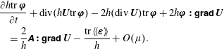 $$\begin{eqnarray}\displaystyle & & \displaystyle \frac{\unicode[STIX]{x2202}h\text{tr}\,\unicode[STIX]{x1D753}}{\unicode[STIX]{x2202}t}+\text{div}(h\boldsymbol{U}\text{tr}\,\unicode[STIX]{x1D753})-2h(\text{div}\,\boldsymbol{U})\text{tr}\,\unicode[STIX]{x1D753}+2h\unicode[STIX]{x1D753}\boldsymbol{ : }\unicode[STIX]{x1D5F4}\unicode[STIX]{x1D5FF}\unicode[STIX]{x1D5EE}\unicode[STIX]{x1D5F1}\,\boldsymbol{U}\nonumber\\ \displaystyle & & \displaystyle \quad =\frac{2}{h}\unicode[STIX]{x1D63C}\boldsymbol{ : }\unicode[STIX]{x1D5F4}\unicode[STIX]{x1D5FF}\unicode[STIX]{x1D5EE}\unicode[STIX]{x1D5F1}\,\boldsymbol{U}-\frac{\text{tr}\,\langle \langle \unicode[STIX]{x1D73A}\rangle \rangle }{h}+O(\unicode[STIX]{x1D707}).\end{eqnarray}$$
The term in
 $\unicode[STIX]{x1D63C}\boldsymbol{ : }\unicode[STIX]{x1D5F4}\unicode[STIX]{x1D5FF}\unicode[STIX]{x1D5EE}\unicode[STIX]{x1D5F1}\,\boldsymbol{U}$
is positive and results in a creation of turbulent energy since
 $\unicode[STIX]{x1D63C}\boldsymbol{ : }\unicode[STIX]{x1D5F4}\unicode[STIX]{x1D5FF}\unicode[STIX]{x1D5EE}\unicode[STIX]{x1D5F1}\,\boldsymbol{U}=2\unicode[STIX]{x1D708}_{T}\Vert \unicode[STIX]{x1D64E}_{\unicode[STIX]{x1D7EC}}\Vert ^{2}+3\unicode[STIX]{x1D708}_{T}(\text{div}\,\boldsymbol{U})^{2}\geqslant 0$
where
 $\Vert \unicode[STIX]{x1D64E}_{\unicode[STIX]{x1D7EC}}\Vert =(\unicode[STIX]{x1D64E}_{\unicode[STIX]{x1D7EC}}:\unicode[STIX]{x1D64E}_{\unicode[STIX]{x1D7EC}})^{1/2}$
. Note that the volume viscosity entails a creation of turbulent energy due to the variations of the water depth which are analogous to compressions or expansions of compressible fluids. These depth variations are characterized by
 $\text{div}\,\boldsymbol{U}$
which is related to the material derivative
 ${\dot{h}}$
by
 ${\dot{h}}=-h\,\text{div}\,\boldsymbol{U}$
.
2.6 Vorticity of the mean flow
Let us denote by
 $J$
the determinant of the enstrophy tensor
 $\unicode[STIX]{x1D753}$
. The Cauchy inequalities imply that
 $J\geqslant 0$
. If the dispersive, viscous and dissipative terms are removed, the remaining system is hyperbolic (Teshukov Reference Teshukov2007) if
 $J\neq 0$
(Richard Reference Richard2013). If the system is restricted to its hyperbolic part, the determinant of the enstrophy tensor satisfies the equation (Teshukov Reference Teshukov2007)
 $$\begin{eqnarray}\frac{\text{D}J}{\text{D}t}=2\,J\text{div}\,\boldsymbol{U},\end{eqnarray}$$
which implies that
 $h^{2}J$
is conserved along the trajectories of the mean flow and can be interpreted as an entropy of the system (Gavrilyuk & Gouin Reference Gavrilyuk and Gouin2012). Also, in the hyperbolic system, if
 $J>0$
at a time
 $t=0$
, then
 $J>0$
at any time
 $t>0$
. A geometrical interpretation of the evolution equation of the tensor
 $h^{2}\unicode[STIX]{x1D753}$
was given in Gavrilyuk & Gouin (Reference Gavrilyuk and Gouin2012) who showed that the eigenvectors of this tensor undergo a rotation similar to a rigid body and form a natural moving frame whose evolution is determined by the mean rate of the deformation tensor. This interpretation can be further specified. Assuming that
 $J\neq 0$
, the tensor
 $\unicode[STIX]{x1D753}$
is invertible. The evolution equation of the inverse tensor
 $\unicode[STIX]{x1D753}^{\boldsymbol{-}\mathbf{1}}$
can be deduced from (2.49). Restricting ourselves again to the hyperbolic part of the equations, this equation can be written
 $$\begin{eqnarray}\frac{\text{D}\unicode[STIX]{x1D753}^{\boldsymbol{-}\mathbf{1}}}{\text{D}t}=-2(\text{div}\,\boldsymbol{U})\unicode[STIX]{x1D753}^{\boldsymbol{-}\mathbf{1}}+\unicode[STIX]{x1D753}^{\boldsymbol{-}\mathbf{1}}\boldsymbol{\cdot }\unicode[STIX]{x1D64E}+\unicode[STIX]{x1D64E}\boldsymbol{\cdot }\unicode[STIX]{x1D753}^{\boldsymbol{-}\mathbf{1}}+\unicode[STIX]{x1D753}^{\boldsymbol{-}\mathbf{1}}\boldsymbol{\cdot }\overline{\overline{\unicode[STIX]{x1D734}}}-\overline{\overline{\unicode[STIX]{x1D734}}}\boldsymbol{\cdot }\unicode[STIX]{x1D753}^{\boldsymbol{-}\mathbf{1}},\end{eqnarray}$$
where the tensor
 $\overline{\overline{\unicode[STIX]{x1D734}}}$
is the mean rotation-rate tensor which is the antisymmetric part of
 $\unicode[STIX]{x1D5F4}\unicode[STIX]{x1D5FF}\unicode[STIX]{x1D5EE}\unicode[STIX]{x1D5F1}\,\boldsymbol{U}$
.
For comparison, we define another tensor that satisfies a similar equation. First we consider two orthogonal infinitesimal vectors
 $\mathbf{d}\boldsymbol{x}_{\mathbf{1}}=\text{d}x_{1}\boldsymbol{e}_{\mathbf{1}}^{\prime }$
and
 $\mathbf{d}\boldsymbol{x}_{\mathbf{2}}=\text{d}x_{2}\boldsymbol{e}_{\mathbf{2}}^{\prime }$
attached to a point of the fluid and transported by the mean flow (
 $\text{d}x_{1}>0$
and
 $\text{d}x_{2}>0$
). They satisfy the equation
 $\text{D}(\mathbf{d}\boldsymbol{x}_{\boldsymbol{i}})/\text{D}t=\unicode[STIX]{x1D5F4}\unicode[STIX]{x1D5FF}\unicode[STIX]{x1D5EE}\unicode[STIX]{x1D5F1}\,\boldsymbol{U}\boldsymbol{\cdot }\mathbf{d}\boldsymbol{x}_{\boldsymbol{i}}$
, (
 $i\in \{1,2\}$
). We define the diagonal tensor
 $\unicode[STIX]{x1D64B}$
as
 $\unicode[STIX]{x1D64B}=\text{d}x_{1}\boldsymbol{e}_{\mathbf{1}}^{\prime }\,\otimes \,\boldsymbol{e}_{\mathbf{1}}^{\prime }+\text{d}x_{2}\boldsymbol{e}_{\mathbf{2}}^{\prime }\,\otimes \,\boldsymbol{e}_{\mathbf{2}}^{\prime }$
. The vectors
 $\boldsymbol{e}_{\mathbf{1}}^{\prime }$
and
 $\boldsymbol{e}_{\mathbf{2}}^{\prime }$
are eigenvectors of
 $\unicode[STIX]{x1D64B}$
and
 $\text{d}x_{1}$
and
 $\text{d}x_{2}$
are eigenvalues. The tensor
 $\unicode[STIX]{x1D64C}$
defined by
 $\unicode[STIX]{x1D64C}=(\unicode[STIX]{x1D64B}\boldsymbol{\cdot }\unicode[STIX]{x1D64B})^{-1}$
can be represented by an ellipse whose semi-major axis is
 $\text{d}x_{1}$
and semi-minor axis is
 $\text{d}x_{2}$
(assuming
 $\text{d}x_{1}>\text{d}x_{2}$
). The following equality pertaining to the tensor
 $\unicode[STIX]{x1D64C}$
can be derived
 $$\begin{eqnarray}\frac{\text{D}\unicode[STIX]{x1D64C}}{\text{D}t}=-2(\text{div}\,\boldsymbol{U})\unicode[STIX]{x1D64C}+\unicode[STIX]{x1D64C}\boldsymbol{\cdot }\unicode[STIX]{x1D64E}+\unicode[STIX]{x1D64E}\boldsymbol{\cdot }\unicode[STIX]{x1D64C}-\unicode[STIX]{x1D64C}\boldsymbol{\cdot }\overline{\overline{\unicode[STIX]{x1D734}}}+\overline{\overline{\unicode[STIX]{x1D734}}}\boldsymbol{\cdot }\unicode[STIX]{x1D64C}.\end{eqnarray}$$
The comparison between (2.57) and (2.58) shows that these equations differ only in that the mean rotation-rate tensor
 $\overline{\overline{\unicode[STIX]{x1D734}}}$
in (2.58) is replaced by
 $-\overline{\overline{\unicode[STIX]{x1D734}}}$
in (2.57). This means that the inverse enstrophy tensor is convected by the mean flow, deformed by the mean strain rate tensor and rotated by the opposite of the mean rotation-rate tensor. Moreover the tensor
 $\unicode[STIX]{x1D753}^{\boldsymbol{-}\mathbf{1}}$
can be represented by an ellipse whose area can be written
 ${\mathcal{A}}=\unicode[STIX]{x03C0}\sqrt{J}$
. The (2.56) implies that
 $$\begin{eqnarray}\frac{1}{{\mathcal{A}}}\frac{\text{D}{\mathcal{A}}}{\text{D}t}=\text{div}\,\boldsymbol{U}.\end{eqnarray}$$
The rate of change of the area of the ellipse is the rate of change of area due to the mean flow (in a three-dimensional space
 $\text{div}\,\boldsymbol{U}$
would be a rate of change of volume). The area of the ellipse associated with
 $\unicode[STIX]{x1D64C}$
satisfies the same equation. It follows that the dilatation, convection and deformation of this ellipse are the same as an infinitesimal ellipse attached to material particles moving with the mean flow but that this ellipse undergoes a rotation with an angular velocity which is exactly the opposite of the local angular velocity of the mean flow.
The vorticity of the mean flow could be defined as
 $\unicode[STIX]{x1D734}=\mathbf{rot}\,\boldsymbol{U}$
but, as the mean flow is two-dimensional, there is only one non-zero component which is in the
 $Oz$
direction and it is better to define the vorticity as
 $$\begin{eqnarray}\unicode[STIX]{x1D6FA}=\overline{\overline{\unicode[STIX]{x1D73A}}}\boldsymbol{ : }\unicode[STIX]{x1D5F4}\unicode[STIX]{x1D5FF}\unicode[STIX]{x1D5EE}\unicode[STIX]{x1D5F1}\,\boldsymbol{U}.\end{eqnarray}$$
In this expression,
 $\overline{\overline{\unicode[STIX]{x1D73A}}}$
is the two-dimensional pseudotensor of Levi-Civita which can be written
 $\overline{\overline{\unicode[STIX]{x1D73A}}}=\overline{\unicode[STIX]{x1D700}}_{ij}\boldsymbol{e}_{\boldsymbol{i}}\,\otimes \,\boldsymbol{e}_{\boldsymbol{j}}$
where
 $\overline{\unicode[STIX]{x1D700}}_{ij}$
is the two-dimensional symbol of Levi-Civita defined by
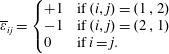 $$\begin{eqnarray}\overline{\unicode[STIX]{x1D700}}_{ij}=\left\{\begin{array}{@{}ll@{}}+1 & \text{if}\;(i,j)=(1\,,2)\\ -1 & \text{if}\;(i,j)=(2\,,1)\\ 0 & \text{if}\;i=j.\end{array}\right.\end{eqnarray}$$
The mean rotation-rate tensor can be written
 $\overline{\overline{\unicode[STIX]{x1D734}}}=-(\unicode[STIX]{x1D6FA}/2)\boldsymbol{e}_{\mathbf{1}}\,\otimes \,\boldsymbol{e}_{\mathbf{2}}+(\unicode[STIX]{x1D6FA}/2)\boldsymbol{e}_{\mathbf{2}}\,\otimes \,\boldsymbol{e}_{\mathbf{1}}$
. Thus it seems that the difference between (2.57) and (2.58) is due to the vorticity of the mean flow and that the tensors
 $\unicode[STIX]{x1D753}^{\boldsymbol{-}\mathbf{1}}$
and
 $\unicode[STIX]{x1D64C}$
satisfy the same equation if the mean flow is irrotational (Debieve, Gouin & Gaviglio Reference Debieve, Gouin and Gaviglio1982).
However an evolution equation of the vorticity of the mean flow can be derived from (2.38). This vorticity equation can be written
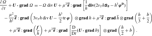 $$\begin{eqnarray}\displaystyle & & \displaystyle \frac{\unicode[STIX]{x2202}\unicode[STIX]{x1D6FA}}{\unicode[STIX]{x2202}t}+\boldsymbol{U}\boldsymbol{\cdot }\mathbf{g}\mathbf{r}\mathbf{a}\mathbf{d}\,\unicode[STIX]{x1D6FA}=-\unicode[STIX]{x1D6FA}\,\text{div}\,\boldsymbol{U}+\unicode[STIX]{x1D707}^{2}\overline{\overline{\unicode[STIX]{x1D73A}}}:\unicode[STIX]{x1D5F4}\unicode[STIX]{x1D5FF}\unicode[STIX]{x1D5EE}\unicode[STIX]{x1D5F1}\left[\frac{1}{h}\mathbf{div}(2\unicode[STIX]{x1D708}_{T}h\unicode[STIX]{x1D64E}_{\unicode[STIX]{x1D7EC}}-h^{3}\unicode[STIX]{x1D753}^{\mathbf{D}})\right]\nonumber\\ \displaystyle & & \displaystyle \quad -\,\frac{\unicode[STIX]{x1D707}^{2}}{h^{2}}\overline{\overline{\unicode[STIX]{x1D73A}}}:\mathbf{g}\mathbf{r}\mathbf{a}\mathbf{d}\left(3\unicode[STIX]{x1D708}_{T}h\,\text{div}\,\boldsymbol{U}-\frac{h^{3}}{2}\text{tr}\,\unicode[STIX]{x1D753}\right)\,\otimes \,\mathbf{g}\mathbf{r}\mathbf{a}\mathbf{d}\,h+\unicode[STIX]{x1D707}^{2}\overline{\overline{\unicode[STIX]{x1D73A}}}:\mathbf{g}\mathbf{r}\mathbf{a}\mathbf{d}\,\ddot{h}\,\otimes \,\mathbf{g}\mathbf{r}\mathbf{a}\mathbf{d}\left(\frac{h}{3}+\frac{b}{2}\right)\nonumber\\ \displaystyle & & \displaystyle \qquad +\,\unicode[STIX]{x1D707}^{2}\overline{\overline{\unicode[STIX]{x1D73A}}}:\unicode[STIX]{x1D5F4}\unicode[STIX]{x1D5FF}\unicode[STIX]{x1D5EE}\unicode[STIX]{x1D5F1}\left(\frac{\boldsymbol{f}}{h}\right)+\unicode[STIX]{x1D707}^{2}\overline{\overline{\unicode[STIX]{x1D73A}}}:\mathbf{g}\mathbf{r}\mathbf{a}\mathbf{d}\left[\frac{\text{D}}{\text{D}t}(\boldsymbol{U}\boldsymbol{\cdot }\mathbf{g}\mathbf{r}\mathbf{a}\mathbf{d}\,b)\right]\,\otimes \,\mathbf{g}\mathbf{r}\mathbf{a}\mathbf{d}\left(\frac{h}{2}+b\right).\end{eqnarray}$$
The decomposition of the enstrophy tensor as the sum of its isotropic (or spherical) part and of its anisotropic (or deviatoric) part is written
 $\unicode[STIX]{x1D753}=(\text{tr}\unicode[STIX]{x1D753})\unicode[STIX]{x1D644}/2+\unicode[STIX]{x1D753}^{\mathbf{D}}$
where
 $\unicode[STIX]{x1D753}^{\mathbf{D}}$
is the deviator of the enstrophy tensor. The compressible character of the equations entails the presence of source terms in this vorticity equation such as the term
 $-\unicode[STIX]{x1D6FA}\,\text{div}\,\boldsymbol{U}$
on the right-hand side of the equation. There are also baroclinic terms which in the three-dimensional usual case would be written
 $-(1/\unicode[STIX]{x1D70C}^{2})\,\mathbf{g}\mathbf{r}\mathbf{a}\mathbf{d}\,\unicode[STIX]{x1D70C}\times \mathbf{g}\mathbf{r}\mathbf{a}\mathbf{d}\,p$
and which here take the form
 $-(1/h^{2})\,\overline{\overline{\unicode[STIX]{x1D73A}}}:\mathbf{g}\mathbf{r}\mathbf{a}\mathbf{d}\,{\mathcal{P}}\,\otimes \,\mathbf{g}\mathbf{r}\mathbf{a}\mathbf{d}\,h$
where
 ${\mathcal{P}}$
is some scalar field (
 $h$
is here analogous to the density
 $\unicode[STIX]{x1D70C}$
). In particular there is a baroclinic term due to the turbulent volume viscosity
 $\unicode[STIX]{x1D701}=3\unicode[STIX]{x1D708}_{T}$
and to the trace of the enstrophy tensor. There are also source terms akin to baroclinic terms due to the dispersion and to the variable bottom. And finally there are source terms due to the first turbulent viscosity and to the deviator of the enstrophy tensor.
This equation shows the big difference between the tensors
 $\unicode[STIX]{x1D753}^{\boldsymbol{-}\mathbf{1}}$
and
 $\unicode[STIX]{x1D64C}$
. Equation (2.58) is only a geometrical description of the variation of
 $\unicode[STIX]{x1D64C}$
while it is transported by the mean flow. The tensor
 $\unicode[STIX]{x1D64C}$
has no influence on the mean flow and is only passively transported. On the contrary, the enstrophy tensor is not only transported and modified by the mean flow, it modifies the mean flow since
 $\unicode[STIX]{x1D753}$
appears in the momentum equation (2.38). This means that (2.49) is a physical equation and not a mere geometrical equation such as (2.58) in spite of the similarity.
Even if the mean rotation-rate tensor has no influence on the trace of the enstrophy tensor nor on the energy, because the terms involving
 $\overline{\overline{\unicode[STIX]{x1D734}}}$
in (2.57) are traceless, it is inconsistent to neglect these terms in the enstrophy tensor equation, assuming that the mean flow is irrotational or weakly rotational, because the enstrophy tensor is a source in the vorticity equation, notably by its deviatoric part. It is also not possible to calculate the enstrophy tensor by replacing (2.49) by an equation of the kind of (2.58) with a hypothesis of a weak vorticity because this one is not tenable given that the enstrophy can create vorticity. Moreover (2.58) has a completely different meaning, is not hyperbolic and has wholly different characteristics.
The presence of the enstrophy tensor, including its deviator, in the vorticity equation (2.62) shows that transfers can happen between the three-dimensional horizontal eddies modelled by the enstrophy tensor and the two-dimensional vertical eddies represented by the vorticity of the mean flow. Our depth-averaged LES approach with a cutoff in the inertial subrange follows the energy cascade from the energy-containing range towards the dissipation range but can describe transfers from the large-scale turbulence with a scale of
 $O(h)$
or smaller (in the water depth) towards the vertical eddies of the average flow with an even bigger scale.
3 Modelling the eddy viscosity and the dissipation tensor
To close the model, two quantities remain to be specified, namely the turbulent viscosity
 $\unicode[STIX]{x1D708}_{T}$
and the averaged dissipation tensor
 $\langle \langle \unicode[STIX]{x1D73A}\rangle \rangle$
. Empirical laws are proposed to determine these two quantities. A correct model of the dissipation should preserve the positivity of the enstrophy tensor and thus of its determinant
 $J$
and of its trace. The determinant can be written
 $J=[(\text{tr}\,\unicode[STIX]{x1D753})^{2}-\unicode[STIX]{x1D753}:\unicode[STIX]{x1D753}]/2$
. Ignoring all terms except the dissipation in the enstrophy equation (2.49) leads to the evolution equations
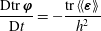 $$\begin{eqnarray}\frac{\text{D}\text{tr}\,\unicode[STIX]{x1D753}}{\text{D}t}=-\frac{\text{tr}\,\langle \langle \unicode[STIX]{x1D73A}\rangle \rangle }{h^{2}}\end{eqnarray}$$
and
 $$\begin{eqnarray}\frac{\text{D}J}{\text{D}t}=-\frac{1}{h^{2}}(\text{tr}\,\unicode[STIX]{x1D753}\,\text{tr}\langle \langle \unicode[STIX]{x1D73A}\rangle \rangle -\unicode[STIX]{x1D753}\boldsymbol{ : }\langle \langle \unicode[STIX]{x1D73A}\rangle \rangle ).\end{eqnarray}$$
A simple way to preserve the positivity of both
 $\text{tr}\,\unicode[STIX]{x1D753}$
and
 $J$
is to have
 $\text{D}\text{tr}\,\unicode[STIX]{x1D753}/\text{D}t=-\text{tr}\,\unicode[STIX]{x1D753}f_{1}$
and
 $\text{D}J/\text{D}t=-Jf_{2}$
where
 $f_{1}$
and
 $f_{2}$
are positive functions depending on the variables of the mean flow. As the equations of the model must satisfy the Galilean invariance, these functions should not depend on
 $\boldsymbol{U}$
. Moreover, they should be invariant in every coordinate systems. This implies that they can depend on
 $h$
and on the two invariants of the tensor,
 $\text{tr}\,\unicode[STIX]{x1D753}$
and
 $J$
. The simplest way is to choose
 $\langle \langle \unicode[STIX]{x1D73A}\rangle \rangle =\unicode[STIX]{x1D753}f(h,\text{tr}\,\unicode[STIX]{x1D753})$
where the function
 $f$
depends only on
 $h$
and
 $\text{tr}\,\unicode[STIX]{x1D753}$
and is obtained by a dimensional analysis. This gives
 $f(h,\text{tr}\,\unicode[STIX]{x1D753})=C_{r}h^{2}\sqrt{\text{tr}\,\unicode[STIX]{x1D753}}$
where
 $C_{r}$
is a dimensionless quantity. The model for the average dissipation is thus
 $$\begin{eqnarray}\langle \langle \unicode[STIX]{x1D73A}\rangle \rangle =C_{r}h^{2}\unicode[STIX]{x1D753}\sqrt{\text{tr}\,\unicode[STIX]{x1D753}}.\end{eqnarray}$$
With this choice the one-dimensional case studied in Kazakova & Richard (Reference Kazakova and Richard2019) is recovered as a particular case. Further, since the turbulent kinetic energy of the model is
 $(h^{2}\text{tr}\,\unicode[STIX]{x1D753})/2$
, the chosen model has the same form as the model proposed by Rotta (Reference Rotta1951) if the dissipation and the turbulent kinetic energy are related with a mixing length proportional to the fluid depth.
The model for the turbulent viscosity is obtained by a similar approach. The eddy viscosity must be the same in every Galilean reference frame and in every coordinate system. It is simpler to assume that
 $\unicode[STIX]{x1D708}_{T}$
depends on
 $h$
and
 $\text{tr}\,\unicode[STIX]{x1D753}$
but not on
 $J$
. A dimensional analysis yields
 $\unicode[STIX]{x1D708}_{T}=C_{p}h^{2}\sqrt{\text{tr}\,\unicode[STIX]{x1D753}}$
where the dimensionless quantity
 $C_{p}$
can be interpreted as the inverse of a turbulent Reynolds number
 $R$
leading to
 $$\begin{eqnarray}\unicode[STIX]{x1D708}_{T}=\frac{h^{2}}{R}\sqrt{\text{tr}\,\unicode[STIX]{x1D753}}.\end{eqnarray}$$
The one-dimensional case (Kazakova & Richard Reference Kazakova and Richard2019) is also recovered as a particular case. This expression of the eddy viscosity based on the turbulent kinetic energy and on a mixing length, which is here proportional to the water depth, is a very classical one (Kolmogorov Reference Kolmogorov1942).
4 Numerical implementation
In the absence of enstrophy, the present model reduces to the classical two-dimensional Green–Naghdi equations. The introduction of this new variable entails a modified pressure law and three supplementary transport equations that can be naturally injected into the hyperbolic part of the system. As a consequence, from a general point of view, this model can be numerically treated in a straightforward manner on the basis of any existing numerical approach dedicated to the Green–Naghdi equations. Naturally, this is even simpler in the one-dimensional case, since the enstrophy tensor equation reduces to a scalar equation. On this basis, preliminary results were obtained by Kazakova & Richard (Reference Kazakova and Richard2019) using an extension of the strategy proposed in Le Métayer, Gavrilyuk & Hank (Reference Le Métayer, Gavrilyuk and Hank2010) for mild slope topographies, allowing the establishment of relevant empirical laws based on the study of solitary waves. In the present work we aim to pursue the efforts towards describing realistic situations, considering a two-dimensional approach on general bathymetries. In addition, and notably for the analysis of periodic waves, we have to think about how to improve the dispersive properties of the proposed model. Before getting through the numerical implementation, we briefly discuss how to address such an issue.
4.1 Constant diagonal formulation
In view of the targeted numerical simulations, we first propose to rewrite the model in an asymptotically equivalent form, allowing us both to improve the dispersive properties and provide a gain in terms of computational cost. To achieve this outcome, we exploit the works proposed by Bonneton et al. (Reference Bonneton, Chazel, Lannes, Marche and Tissier2011), followed later by Lannes & Marche (Reference Lannes and Marche2015), mainly for purposes of computational efficiency. The present section merely consists in verifying that the current model enters into the appropriate formalism. Consequently we shall not discuss all technical aspects, and refer to the aforementioned references for more details.
As is the case when dealing with Boussinesq-type models, the numerical challenge stands in the treatment of the discharge equation, due to the presence of high-order derivatives (up to third order) and second-order non-stationary terms appearing through the material derivative. This last point has heavy practical consequences since it results in the inversion of a time-dependent elliptic operator which couples the velocity components.
The model is constituted by (2.23), (2.38) and (2.49). In all applications presented in the present paper, the friction term was not needed to reach a good agreement with the experimental measures. Consequently in the following
 $\boldsymbol{f}=0$
. These equations, written with the components of
 $\boldsymbol{U}$
and
 $\unicode[STIX]{x1D753}$
, are collected for convenience’ sake in appendix B. As mentioned before, this model reduces to the standard Green–Naghdi equations with a modified pressure law, supplemented by the transport of the enstrophy tensor. We hence inherit the same technical difficulties as discussed just before, concentrated in the discharge evolution. As a consequence, in what follows we will only focus on the momentum equation.
As a first remark, adapting the notations used in Bonneton et al. (Reference Bonneton, Chazel, Lannes, Marche and Tissier2011), we can express the average velocity equation (2.38) as
 $$\begin{eqnarray}(\unicode[STIX]{x1D644}+\unicode[STIX]{x1D707}^{2}\unicode[STIX]{x1D64F})\frac{\unicode[STIX]{x2202}\boldsymbol{U}}{\unicode[STIX]{x2202}t}+\boldsymbol{U}\boldsymbol{\cdot }\unicode[STIX]{x1D5F4}\unicode[STIX]{x1D5FF}\unicode[STIX]{x1D5EE}\unicode[STIX]{x1D5F1}\,\boldsymbol{U}+\mathbf{g}\mathbf{r}\mathbf{a}\mathbf{d}(h+b)+\frac{\unicode[STIX]{x1D707}^{2}}{h}\mathbf{div}(h^{3}\unicode[STIX]{x1D753}-h\unicode[STIX]{x1D63C})+\unicode[STIX]{x1D707}^{2}\boldsymbol{Q}_{\boldsymbol{ 0}}=O(\unicode[STIX]{x1D707}^{3}).\end{eqnarray}$$
In this expression
 $\unicode[STIX]{x1D644}$
is the identity operator,
 $\unicode[STIX]{x1D64F}$
is a linear operator depending on
 $h$
and
 $b$
and defined by
 $$\begin{eqnarray}\displaystyle \unicode[STIX]{x1D64F}\,\boldsymbol{W} & = & \displaystyle -\frac{1}{3h}\mathbf{g}\mathbf{r}\mathbf{a}\mathbf{d}(h^{3}\text{div}\boldsymbol{W})-\frac{h}{2}\text{div}\,\boldsymbol{W}\mathbf{g}\mathbf{r}\mathbf{a}\mathbf{d}\,b+\frac{1}{2h}\mathbf{g}\mathbf{r}\mathbf{a}\mathbf{d}(h^{2}\mathbf{g}\mathbf{r}\mathbf{a}\mathbf{d}\,b\boldsymbol{\cdot }\boldsymbol{W})\nonumber\\ \displaystyle & & \displaystyle +\,(\mathbf{g}\mathbf{r}\mathbf{a}\mathbf{d}\,b\boldsymbol{\cdot }\boldsymbol{W})\mathbf{g}\mathbf{r}\mathbf{a}\mathbf{d}\,b\end{eqnarray}$$
for any vector field
 $\boldsymbol{W}$
and
 $$\begin{eqnarray}\displaystyle \boldsymbol{Q}_{\mathbf{0}} & = & \displaystyle -\frac{1}{3h}\mathbf{g}\mathbf{r}\mathbf{a}\mathbf{d}\{h^{3}[\text{div}(\boldsymbol{U}\text{div}\,\boldsymbol{U})-2(\text{div}\,\boldsymbol{U})^{2}]\}+[\boldsymbol{U}\boldsymbol{\cdot }\mathbf{g}\mathbf{r}\mathbf{a}\mathbf{d}(\boldsymbol{U}\boldsymbol{\cdot }\mathbf{g}\mathbf{r}\mathbf{a}\mathbf{d}\,b)]\mathbf{g}\mathbf{r}\mathbf{a}\mathbf{d}\,b\nonumber\\ \displaystyle & & \displaystyle -\,\frac{h}{2}[\text{div}(\boldsymbol{U}\text{div}\,\boldsymbol{U})-2(\text{div}\,\boldsymbol{U})^{2}]\mathbf{g}\mathbf{r}\mathbf{a}\mathbf{d}\,b+\frac{1}{2h}\mathbf{g}\mathbf{r}\mathbf{a}\mathbf{d}[h^{2}\boldsymbol{U}\boldsymbol{\cdot }\mathbf{g}\mathbf{r}\mathbf{a}\mathbf{d}(\boldsymbol{U}\boldsymbol{\cdot }\mathbf{g}\mathbf{r}\mathbf{a}\mathbf{d}\,b)].\qquad\end{eqnarray}$$
Introducing the notation
 $$\begin{eqnarray}\boldsymbol{Q}_{\mathbf{0}}^{\prime }=\boldsymbol{Q}_{\boldsymbol{ 0}}+\frac{1}{h}\mathbf{div}(h^{3}\unicode[STIX]{x1D753}-h\unicode[STIX]{x1D63C}),\end{eqnarray}$$
the previous equation becomes
 $$\begin{eqnarray}(\unicode[STIX]{x1D644}+\unicode[STIX]{x1D707}^{2}\unicode[STIX]{x1D64F})\frac{\unicode[STIX]{x2202}\boldsymbol{U}}{\unicode[STIX]{x2202}t}+\boldsymbol{U}\boldsymbol{\cdot }\,\unicode[STIX]{x1D5F4}\unicode[STIX]{x1D5FF}\unicode[STIX]{x1D5EE}\unicode[STIX]{x1D5F1}\,\boldsymbol{U}+\mathbf{g}\mathbf{r}\mathbf{a}\mathbf{d}(h+b)+\unicode[STIX]{x1D707}^{2}\boldsymbol{Q}_{\boldsymbol{ 0}}^{\prime }=O(\unicode[STIX]{x1D707}^{3}),\end{eqnarray}$$
and we can reproduce the arguments employed in Bonneton et al. (Reference Bonneton, Chazel, Lannes, Marche and Tissier2011) to obtain the equation
 $$\begin{eqnarray}(\unicode[STIX]{x1D644}+\unicode[STIX]{x1D707}^{2}\unicode[STIX]{x1D64F})\left(\frac{\unicode[STIX]{x2202}\boldsymbol{U}}{\unicode[STIX]{x2202}t}+\boldsymbol{U}\boldsymbol{\cdot }\unicode[STIX]{x1D5F4}\unicode[STIX]{x1D5FF}\unicode[STIX]{x1D5EE}\unicode[STIX]{x1D5F1}\,\boldsymbol{U}\right)+\mathbf{g}\mathbf{r}\mathbf{a}\mathbf{d}(h+b)+\unicode[STIX]{x1D707}^{2}\boldsymbol{Q}_{\boldsymbol{ 1}}=O(\unicode[STIX]{x1D707}^{3}),\end{eqnarray}$$
where
 $$\begin{eqnarray}\boldsymbol{Q}_{\mathbf{1}}=\boldsymbol{Q}_{\mathbf{0}}^{\prime }-\unicode[STIX]{x1D64F}(\boldsymbol{U}\boldsymbol{\cdot }\unicode[STIX]{x1D5F4}\unicode[STIX]{x1D5FF}\unicode[STIX]{x1D5EE}\unicode[STIX]{x1D5F1}\,\boldsymbol{U}).\end{eqnarray}$$
Denoting by
 $(\unicode[STIX]{x1D644}+\unicode[STIX]{x1D707}^{2}\unicode[STIX]{x1D64F})^{-1}$
the inverse operator of
 $(\unicode[STIX]{x1D644}+\unicode[STIX]{x1D707}^{2}\unicode[STIX]{x1D64F})$
, this equation can be written
 $$\begin{eqnarray}\frac{\unicode[STIX]{x2202}\boldsymbol{U}}{\unicode[STIX]{x2202}t}+\boldsymbol{U}\boldsymbol{\cdot }\unicode[STIX]{x1D5F4}\unicode[STIX]{x1D5FF}\unicode[STIX]{x1D5EE}\unicode[STIX]{x1D5F1}\,\boldsymbol{U}+(\unicode[STIX]{x1D644}+\unicode[STIX]{x1D707}^{2}\unicode[STIX]{x1D64F})^{-1}[\mathbf{g}\mathbf{r}\mathbf{a}\mathbf{d}(h+b)+\unicode[STIX]{x1D707}^{2}\boldsymbol{Q}_{\boldsymbol{ 1}}]=O(\unicode[STIX]{x1D707}^{3}).\end{eqnarray}$$
As highlighted by Lannes & Marche (Reference Lannes and Marche2015), this formulation has two main advantages, namely it does not require the computation of third-order derivatives, and the presence of the operator
 $(\unicode[STIX]{x1D644}+\unicode[STIX]{x1D707}^{2}\unicode[STIX]{x1D64F})$
makes the model stable with respect to high frequency perturbations. Nevertheless, a remaining major drawback is the necessity of inverting this operator, since it is time dependent and involves a coupling between the velocity components. Starting form the dimensionless mass equation and a velocity equation under the form (4.6), Lannes & Marche (Reference Lannes and Marche2015) reached the following so-called ‘constant diagonal’ formulation of the momentum equations, which reads, in the present context:
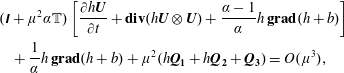 $$\begin{eqnarray}\displaystyle & & \displaystyle (\unicode[STIX]{x1D644}+\unicode[STIX]{x1D707}^{2}\unicode[STIX]{x1D6FC}\mathbb{T})\left[\frac{\unicode[STIX]{x2202}h\boldsymbol{U}}{\unicode[STIX]{x2202}t}+\mathbf{div}(h\boldsymbol{U}\,\otimes \,\boldsymbol{U})+\frac{\unicode[STIX]{x1D6FC}-1}{\unicode[STIX]{x1D6FC}}h\,\mathbf{g}\mathbf{r}\mathbf{a}\mathbf{d}(h+b)\right]\nonumber\\ \displaystyle & & \displaystyle \quad +\,\frac{1}{\unicode[STIX]{x1D6FC}}h\,\mathbf{g}\mathbf{r}\mathbf{a}\mathbf{d}(h+b)+\unicode[STIX]{x1D707}^{2}(h\boldsymbol{Q}_{\boldsymbol{ 1}}+h\boldsymbol{Q}_{\mathbf{2}}+\boldsymbol{Q}_{\mathbf{3}})=O(\unicode[STIX]{x1D707}^{3}),\end{eqnarray}$$
where the operator
 $\mathbb{T}$
only depends on a given water depth at rest
 $h_{0}$
and has a time-independent diagonal structure since
 $$\begin{eqnarray}\mathbb{T}\,\boldsymbol{W}=-\frac{1}{3}\mathbf{div}\left[h_{0}^{3}\,\unicode[STIX]{x1D5F4}\unicode[STIX]{x1D5FF}\unicode[STIX]{x1D5EE}\unicode[STIX]{x1D5F1}\frac{\boldsymbol{W}}{h_{0}}\right]=-\frac{1}{3}\frac{\unicode[STIX]{x2202}}{\unicode[STIX]{x2202}x_{j}}\left(h_{0}^{3}\frac{\unicode[STIX]{x2202}}{\unicode[STIX]{x2202}x_{j}}\frac{W_{i}}{h_{0}}\right)\boldsymbol{e}_{\boldsymbol{i}}\end{eqnarray}$$
for any vector field
 $\boldsymbol{W}=W_{i}\boldsymbol{e}_{\boldsymbol{i}}$
. The auxiliary quantities are defined as follows:
 $$\begin{eqnarray}\displaystyle \boldsymbol{Q}_{\mathbf{2}} & = & \displaystyle h\,\unicode[STIX]{x1D5F4}\unicode[STIX]{x1D5FF}\unicode[STIX]{x1D5EE}\unicode[STIX]{x1D5F1}[\overline{\overline{\unicode[STIX]{x1D73A}}}\boldsymbol{\cdot }\mathbf{g}\mathbf{r}\mathbf{a}\mathbf{d}(h+b)]\boldsymbol{\cdot }\overline{\overline{\unicode[STIX]{x1D73A}}}\boldsymbol{\cdot }\mathbf{g}\mathbf{r}\mathbf{a}\mathbf{d}\,h-\frac{1}{2h}\mathbf{g}\mathbf{r}\mathbf{a}\mathbf{d}[h^{2}\mathbf{g}\mathbf{r}\mathbf{a}\mathbf{d}\,b\boldsymbol{\cdot }\mathbf{g}\mathbf{r}\mathbf{a}\mathbf{d}(h+b)]\nonumber\\ \displaystyle & & \displaystyle +\,\frac{h}{2}\mathbf{g}\mathbf{r}\mathbf{a}\mathbf{d}\,b\unicode[STIX]{x1D6E5}(h+b)-[\mathbf{g}\mathbf{r}\mathbf{a}\mathbf{d}\,b\boldsymbol{\cdot }\mathbf{g}\mathbf{r}\mathbf{a}\mathbf{d}(h+b)]\mathbf{g}\mathbf{r}\mathbf{a}\mathbf{d}\,b+O(\unicode[STIX]{x1D707}^{2})\end{eqnarray}$$
and
 $$\begin{eqnarray}\boldsymbol{Q}_{\mathbf{3}}=\unicode[STIX]{x1D64E}\{(\unicode[STIX]{x1D644}+\unicode[STIX]{x1D707}^{2}\unicode[STIX]{x1D6FC}\mathbb{T})^{-1}[h\,\mathbf{g}\mathbf{r}\mathbf{a}\mathbf{d}(h+b)]\},\end{eqnarray}$$
where
 $\unicode[STIX]{x1D64E}$
is an operator defined as
 $$\begin{eqnarray}\unicode[STIX]{x1D64E}\{\boldsymbol{W}\}={\textstyle \frac{1}{6}}\mathbf{g}\mathbf{r}\mathbf{a}\mathbf{d}(h^{2}-h_{0}^{2})\boldsymbol{\cdot }\unicode[STIX]{x1D5F4}\unicode[STIX]{x1D5FF}\unicode[STIX]{x1D5EE}\unicode[STIX]{x1D5F1}\,\boldsymbol{W}+{\textstyle \frac{1}{3}}(h^{2}-h_{0}^{2})\unicode[STIX]{x0394}\boldsymbol{W}-{\textstyle \frac{1}{6}}\unicode[STIX]{x1D6E5}(h^{2}-h_{0}^{2})\boldsymbol{W}\end{eqnarray}$$
for a generic smooth enough vector field
 $\boldsymbol{W}$
. The role of the constant
 $\unicode[STIX]{x1D6FC}$
, initially introduced by Bonneton et al. (Reference Bonneton, Chazel, Lannes, Marche and Tissier2011), is precisely to improve the dispersive properties of the model (namely, to provide a better matching with respect to the linear Stokes theory). Following the works previously mentioned, we take
 $\unicode[STIX]{x1D6FC}=1.159$
in our numerical experiments. Note that in the above formulation (4.9), the only difference with the original work is the expression of
 $\boldsymbol{Q}_{\mathbf{1}}$
(4.7), which through (4.4) also contains the conservative and viscous terms related to the enstrophy. Going back to variables with dimensions, (4.9) becomes:
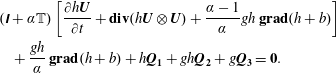 $$\begin{eqnarray}\displaystyle & & \displaystyle (\unicode[STIX]{x1D644}+\unicode[STIX]{x1D6FC}\mathbb{T})\left[\frac{\unicode[STIX]{x2202}h\boldsymbol{U}}{\unicode[STIX]{x2202}t}+\mathbf{div}(h\boldsymbol{U}\,\otimes \,\boldsymbol{U})+\frac{\unicode[STIX]{x1D6FC}-1}{\unicode[STIX]{x1D6FC}}gh\,\mathbf{g}\mathbf{r}\mathbf{a}\mathbf{d}(h+b)\right]\nonumber\\ \displaystyle & & \displaystyle \quad +\,\frac{gh}{\unicode[STIX]{x1D6FC}}\,\mathbf{g}\mathbf{r}\mathbf{a}\mathbf{d}(h+b)+h\boldsymbol{Q}_{\mathbf{1}}+gh\boldsymbol{Q}_{\mathbf{2}}+g\boldsymbol{Q}_{\mathbf{3}}=\mathbf{0}.\end{eqnarray}$$
Finally, following what has been done in Duran & Marche (Reference Duran and Marche2017) we reformulate the previous equation as:
 $$\begin{eqnarray}\frac{\unicode[STIX]{x2202}h\boldsymbol{U}}{\unicode[STIX]{x2202}t}+\mathbf{div}(h\boldsymbol{U}\,\otimes \,\boldsymbol{U}+h^{3}\unicode[STIX]{x1D753})+gh\,\mathbf{g}\mathbf{r}\mathbf{a}\mathbf{d}(h+b)+\boldsymbol{D}=\mathbf{0},\end{eqnarray}$$
where
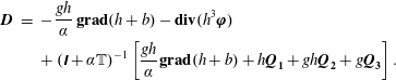 $$\begin{eqnarray}\displaystyle \boldsymbol{D} & = & \displaystyle -\frac{gh}{\unicode[STIX]{x1D6FC}}\,\mathbf{g}\mathbf{r}\mathbf{a}\mathbf{d}(h+b)-\mathbf{div}(h^{3}\unicode[STIX]{x1D753})\nonumber\\ \displaystyle & & \displaystyle +\,(\unicode[STIX]{x1D644}+\unicode[STIX]{x1D6FC}\mathbb{T})^{-1}\left[\frac{gh}{\unicode[STIX]{x1D6FC}}\mathbf{g}\mathbf{r}\mathbf{a}\mathbf{d}(h+b)+h\boldsymbol{Q}_{\mathbf{1}}+gh\boldsymbol{Q}_{\mathbf{2}}+g\boldsymbol{Q}_{\mathbf{3}}\right].\end{eqnarray}$$
This formulation is asymptotically equivalent to the original model presented in appendix B but with improved dispersive properties. Without this treatment, dispersive properties (which are the same as those of the Green–Naghdi equations) are accurate up to
 $kh_{0}\simeq 1$
(where
 $k$
is the wavenumber). With these improvement techniques the results are accurate until
 $kh_{0}\simeq 4$
for the phase celerity,
 $kh_{0}\simeq 2.5$
for the group velocity and
 $kh_{0}\simeq 2$
for the shoaling gradient (see Chazel, Lannes & Marche Reference Chazel, Lannes and Marche2011).
4.2 Pre-balanced formulation
In this work, numerical investigations will be based on the high-order discontinuous Galerkin approach developed by Duran & Marche (Reference Duran and Marche2017). This approach directly applies to (4.15) with a preliminary rewriting of the hyperbolic part with the prospect of balancing well the properties. This approach extends the 1-D works introduced by Liang & Marche (Reference Liang and Marche2009) for the shallow-water (Saint-Venant) equations, in the context of unstructured high-order discretizations. The key idea is to reformulate the hydrostatic pressure term as
 $$\begin{eqnarray}gh\,\mathbf{g}\mathbf{r}\mathbf{a}\mathbf{d}(h+b)=\frac{g}{2}\mathbf{g}\mathbf{r}\mathbf{a}\mathbf{d}(Z^{2}-2Zb)+gZ\,\mathbf{g}\mathbf{r}\mathbf{a}\mathbf{d}\,b.\end{eqnarray}$$
Then we denote the vector solution
 $\boldsymbol{W}=(Z,h\boldsymbol{U}^{\text{T}},h\unicode[STIX]{x1D711}_{11},h\unicode[STIX]{x1D711}_{12},h\unicode[STIX]{x1D711}_{22})^{\text{T}}$
, and recast (2.23), (4.15) and (2.49) in the compact form:
 $$\begin{eqnarray}\frac{\unicode[STIX]{x2202}\boldsymbol{W}}{\unicode[STIX]{x2202}t}+\mathbf{div}\,\mathbb{F}(\boldsymbol{W},b)+\mathbb{D}(\boldsymbol{W},b)=\mathbb{S}(\boldsymbol{W},b).\end{eqnarray}$$
This system features five equations: the scalar conservation equation of mass (first equation corresponding to (2.23)), the vector balance equation of momentum (second equation corresponding to (4.15)) and three scalar equations for the three independent components of the enstrophy tensor (three last equations corresponding to (2.49)). The flux
 $\mathbb{F}$
and the dispersive term
 $\mathbb{D}$
are defined by
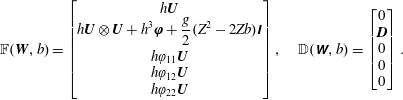 $$\begin{eqnarray}\mathbb{F}(\boldsymbol{W},b)=\left[\begin{array}{@{}c@{}}h\boldsymbol{U}\\ \displaystyle h\boldsymbol{U}\,\otimes \,\boldsymbol{U}+h^{3}\unicode[STIX]{x1D753}+{\displaystyle \frac{g}{2}}(Z^{2}-2Zb)\unicode[STIX]{x1D644}\\ h\unicode[STIX]{x1D711}_{11}\boldsymbol{U}\\ h\unicode[STIX]{x1D711}_{12}\boldsymbol{U}\\ h\unicode[STIX]{x1D711}_{22}\boldsymbol{U}\\ \end{array}\right],\quad \mathbb{D}(\unicode[STIX]{x1D652},b)=\left[\begin{array}{@{}c@{}}0\\ \boldsymbol{D}\\ 0\\ 0\\ 0\end{array}\right].\end{eqnarray}$$
The dispersive
 $\mathbb{R}^{2}$
-valued term
 $\boldsymbol{D}$
is defined by (4.16), and the source term by
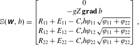 $$\begin{eqnarray}\mathbb{S}(\unicode[STIX]{x1D652},b)=\left[\begin{array}{@{}c@{}}0\\ -gZ\,\mathbf{g}\boldsymbol{ r}\boldsymbol{ a}\boldsymbol{ d}\,b\\ R_{11}+E_{11}-C_{r}h\unicode[STIX]{x1D711}_{11}\sqrt{\unicode[STIX]{x1D711}_{11}+\unicode[STIX]{x1D711}_{22}}\\ R_{12}+E_{12}-C_{r}h\unicode[STIX]{x1D711}_{12}\sqrt{\unicode[STIX]{x1D711}_{11}+\unicode[STIX]{x1D711}_{22}}\\ R_{22}+E_{22}-C_{r}h\unicode[STIX]{x1D711}_{22}\sqrt{\unicode[STIX]{x1D711}_{11}+\unicode[STIX]{x1D711}_{22}}\end{array}\right],\end{eqnarray}$$
with
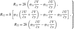 $$\begin{eqnarray}\left.\begin{array}{@{}c@{}}\displaystyle R_{11}=2h\left(\unicode[STIX]{x1D711}_{11}{\displaystyle \frac{\unicode[STIX]{x2202}V}{\unicode[STIX]{x2202}y}}-\unicode[STIX]{x1D711}_{12}{\displaystyle \frac{\unicode[STIX]{x2202}U}{\unicode[STIX]{x2202}y}}\right),\\ \displaystyle R_{12}=h\left[\unicode[STIX]{x1D711}_{12}\left({\displaystyle \frac{\unicode[STIX]{x2202}U}{\unicode[STIX]{x2202}x}}+{\displaystyle \frac{\unicode[STIX]{x2202}V}{\unicode[STIX]{x2202}y}}\right)-\unicode[STIX]{x1D711}_{11}{\displaystyle \frac{\unicode[STIX]{x2202}V}{\unicode[STIX]{x2202}x}}-\unicode[STIX]{x1D711}_{22}{\displaystyle \frac{\unicode[STIX]{x2202}U}{\unicode[STIX]{x2202}y}}\right],\\ \displaystyle R_{22}=2h\left(\unicode[STIX]{x1D711}_{22}{\displaystyle \frac{\unicode[STIX]{x2202}U}{\unicode[STIX]{x2202}x}}-\unicode[STIX]{x1D711}_{12}{\displaystyle \frac{\unicode[STIX]{x2202}V}{\unicode[STIX]{x2202}x}}\right)\end{array}\right\}\end{eqnarray}$$
and
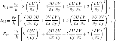 $$\begin{eqnarray}\left.\begin{array}{@{}c@{}}\displaystyle E_{11}={\displaystyle \frac{\unicode[STIX]{x1D708}_{T}}{h}}\left[8\left({\displaystyle \frac{\unicode[STIX]{x2202}U}{\unicode[STIX]{x2202}x}}\right)^{2}+4{\displaystyle \frac{\unicode[STIX]{x2202}U}{\unicode[STIX]{x2202}x}}{\displaystyle \frac{\unicode[STIX]{x2202}V}{\unicode[STIX]{x2202}y}}+2{\displaystyle \frac{\unicode[STIX]{x2202}U}{\unicode[STIX]{x2202}y}}{\displaystyle \frac{\unicode[STIX]{x2202}V}{\unicode[STIX]{x2202}x}}+2\left({\displaystyle \frac{\unicode[STIX]{x2202}U}{\unicode[STIX]{x2202}y}}\right)^{2}\right],\\ \displaystyle E_{12}={\displaystyle \frac{\unicode[STIX]{x1D708}_{T}}{h}}\left[3\left({\displaystyle \frac{\unicode[STIX]{x2202}U}{\unicode[STIX]{x2202}x}}{\displaystyle \frac{\unicode[STIX]{x2202}U}{\unicode[STIX]{x2202}y}}+{\displaystyle \frac{\unicode[STIX]{x2202}V}{\unicode[STIX]{x2202}x}}{\displaystyle \frac{\unicode[STIX]{x2202}V}{\unicode[STIX]{x2202}y}}\right)+5\left({\displaystyle \frac{\unicode[STIX]{x2202}U}{\unicode[STIX]{x2202}x}}{\displaystyle \frac{\unicode[STIX]{x2202}V}{\unicode[STIX]{x2202}x}}+{\displaystyle \frac{\unicode[STIX]{x2202}U}{\unicode[STIX]{x2202}y}}{\displaystyle \frac{\unicode[STIX]{x2202}V}{\unicode[STIX]{x2202}y}}\right)\right],\\ \displaystyle E_{22}={\displaystyle \frac{\unicode[STIX]{x1D708}_{T}}{h}}\left[8\left({\displaystyle \frac{\unicode[STIX]{x2202}V}{\unicode[STIX]{x2202}y}}\right)^{2}+4{\displaystyle \frac{\unicode[STIX]{x2202}U}{\unicode[STIX]{x2202}x}}{\displaystyle \frac{\unicode[STIX]{x2202}V}{\unicode[STIX]{x2202}y}}+2{\displaystyle \frac{\unicode[STIX]{x2202}U}{\unicode[STIX]{x2202}y}}{\displaystyle \frac{\unicode[STIX]{x2202}V}{\unicode[STIX]{x2202}x}}+2\left({\displaystyle \frac{\unicode[STIX]{x2202}V}{\unicode[STIX]{x2202}x}}\right)^{2}\right].\end{array}\right\}\end{eqnarray}$$
Note that the flux function
 $\mathbb{F}$
in (4.18) allows for a clear decoupling between the hyperbolic and dispersive parts of the system. The system (4.18) is the final set of equations which was solved numerically for all test cases.
4.3 Discrete formulation
We now turn to the numerical scheme, which consists of a direct extension of the works of Duran & Marche (Reference Duran and Marche2017). As a consequence, we shall not go into detail here, and refer to this paper for an exhaustive description. The main principles of this numerical scheme are given in appendix C. An example of a regular triangular mesh used in the numerical computations is given in figure 2. Overall, the main numerical challenge stands in the computation of the components of
 $\mathbb{D}$
, which involves the resolution of a global linear system. As previously stated, in our case this task is considerably alleviated since the elliptic operator appearing in (4.15) is time independent and allows us to decouple the evolution of the velocity components. The computation of this term follows the protocol described in Duran & Marche (Reference Duran and Marche2017), based on the use of local discontinuous Galerkin fluxes (Cockburn & Shu Reference Cockburn and Shu1998) to build the first- and second-order differential operators. We refer to the above papers for technical details. As concerns the enstrophy transport, the conservative terms are treated in the hyperbolic stage, according to (4.18), while the associated source terms are computed in a collocated framework with direct nodal products, in the same way as those of the momentum equations. Classically, advancing in time will be carried out by standard high-order strong stability preserving Runge–Kutta (SSP-RK) algorithms, following the original work.
Example of regular mesh.
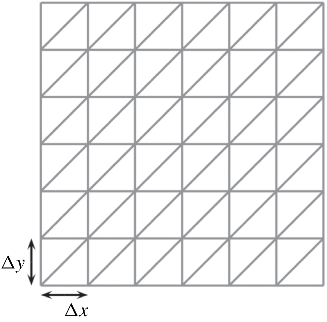
5 Wave breaking
Preliminary results of Part 1 (Kazakova & Richard Reference Kazakova and Richard2019) for solitary waves showed that the activation of the eddy viscosity from the beginning of the computation may decrease prematurely the wave amplitude in the shoaling zone if the initial nonlinearity is too high. This necessitated the use of a breaking criterion in these cases to activate the turbulent viscosity at the breaking point. On the contrary, for solitary waves with an initially small nonlinearity, no breaking criterion was needed and the eddy viscosity was activated from the beginning of the computation in the shoaling zone and the breaking process was predicted naturally as a sudden growth of the enstrophy.
As a consequence, for now, and in the philosophy of other existing strategies, this compels us to introduce a breaking criterion in order to activate the eddy viscosity only in eligible areas. Naturally, the different criteria of the literature mentioned in the introduction can be used to turn on viscosity terms and generate enstrophy only when needed. As for hybrid or ad hoc viscosity methods, this entails the introduction of a discontinuity in the momentum equations in the neighbourhood of the breaking area. From a general viewpoint, this can be a source of numerical instabilities, especially if the discretization parameters are not chosen appropriately. In the present case, the viscous terms being expressed in terms of the enstrophy, they are subject to a regular growth localized in a very thin region surrounding the breaking point, allowing us to introduce the turbulent effects in a smooth way. Further, this behaviour makes the model less sensitive with respect to the mask width in which viscous terms are activated.
Another detection strategy, proposed by Kazakova & Richard (Reference Kazakova and Richard2019) for solitary waves, consists of using the enstrophy itself to detect wave breaking. Indeed, this quantity is intrinsically linked to turbulent effects and can be used as a relevant tool to predict the development of turbulent structures. This leads to the introduction of a new quantity, referred to as virtual enstrophy, which quantifies the amount of enstrophy that the model is potentially able to produce. As in the original work, the virtual enstrophy is computed at each time step as the real enstrophy, but without any feedback on the evolution of the other variables. Then, breaking points can be identified as those where the virtual enstrophy is high enough, which also imposes the introduction of an appropriate threshold. Once this threshold is exceeded, the turbulent viscosity is activated in the neighbourhood of the incriminated cells in order to produce the effective enstrophy to handle wave breaking, in the same manner as for the classical breaking criteria previously mentioned. Classically, a slope limiter is applied in these areas (Cockburn & Shu Reference Cockburn and Shu1998), notably to damp the brutal entropy variations. Note that in the 1-D case studied in Part 1, the enstrophy has only one component. The viscosity is activated when the scalar virtual enstrophy exceeds the threshold value. In the 2-D case studied in the present paper, the enstrophy is a tensor and the threshold value applies now to the trace of the virtual enstrophy. Note that this strategy naturally implies a non-zero value as initial data for all diagonal components of the enstrophy. Following Part 1, this value will be taken to be
 $10^{-10}~\text{s}^{-2}$
in our numerical tests.
The first test case (§ 6.1) is only used to validate the numerical scheme. The problem is to calculate the known analytical solution of a soliton with a constant enstrophy in the absence of dissipation. The test cases 2, 4 and 5 (§ 6.2, §6.4 and §6.5 respectively) deal with solitary waves and the same breaking criteria established in Part 1 are used. We denote by
 $\unicode[STIX]{x1D74D}$
the virtual enstrophy tensor. It satisfies the same equation (2.49) as
 $\unicode[STIX]{x1D753}$
except that in the equation of
 $\unicode[STIX]{x1D74D}$
the eddy viscosity is always activated. Note that in the other equations, the tensor which appears is still
 $\unicode[STIX]{x1D753}$
, not
 $\unicode[STIX]{x1D74D}$
, so that the virtual enstrophy has no effect on the other quantities. The eddy viscosity is activated in the other equations of the model if
 $\text{tr}\,\unicode[STIX]{x1D74D}>\unicode[STIX]{x1D713}_{0}$
where
 $\unicode[STIX]{x1D713}_{0}$
is the breaking threshold which is given by the empirical law of Part 1 (Kazakova & Richard Reference Kazakova and Richard2019)
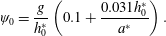 $$\begin{eqnarray}\unicode[STIX]{x1D713}_{0}=\frac{g}{h_{0}^{\ast }}\left(0.1+{\displaystyle \frac{0.031h_{0}^{\ast }}{a^{\ast }}}\right).\end{eqnarray}$$
In this expression,
 $h_{0}^{\ast }$
and
 $a^{\ast }$
are respectively the initial still-water depth and the initial amplitude of the solitary wave. This expression applies if the initial nonlinearity
 $a^{\ast }/h_{0}^{\ast }>0.05$
which is the case in all three test cases. The eddy viscosity is then calculated with the empirical law established in Part 1 for the Reynolds number
 $R$
which appears in (3.4)
 $$\begin{eqnarray}R=0.85+60s,\end{eqnarray}$$
where
 $s$
is the bed slope. In the cases of a variable slope, the value of this Reynolds number can be estimated locally, depending on the local slope, but a numerical investigation showed that a constant value based on an average slope, intermediate between the highest and lowest slopes, can be used without changing significantly the results. This is due to the relatively weak sensitivity of the model to the precise values of the parameters.
The test case 3 (§ 6.3) is the only one to deal with a wave train. The initial nonlinearity is small enough to simulate all wave propagations, including the breaking initiation and termination, without any breaking criterion. The Reynolds number
 $R$
of (3.4) is calculated with the result found in Part 1 for solitary waves with a small initial nonlinearity i.e.
 $5<R<10$
. The value
 $R=7.5$
was used although another value in this interval gives almost the same results. The determination of the general empirical laws for
 $\unicode[STIX]{x1D713}_{0}$
and
 $R$
for wave trains will necessitate a thorough investigation which is left for a future work. Of course, it is always possible to tune all parameters case by case to match the experimental measures but this method would prevent the model being predictive.
As in Part 1 the coefficient
 $C_{r}$
is taken equal to
 $0.48$
in all cases. The values of the parameters used for each test case are gathered in table 1 although other choices are possible for the cases 4 and 5 (see the explanations in §§ 6.4 and 6.5) because the slope is not constant.
Values of the parameters used for each test case.
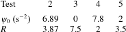
6 Numerical results
6.1 Augmented solitary wave
As a preliminary test we validate the ability of the scheme to capture an analytical solution, in the absence of topography and without breaking effects. In a recent work, Richard & Gavrilyuk (Reference Richard and Gavrilyuk2015) showed the existence of solitary waves with non-trivial constant enstrophy profiles as exact solutions to the model. Considering a reference enstrophy
 $\unicode[STIX]{x1D711}_{0}$
, the corresponding relative amplitude
 $\tilde{a}=a/h_{0}$
, where the amplitude
 $a$
of the wave is the maximum value of
 $\unicode[STIX]{x1D702}$
(see figure 1), is
 $$\begin{eqnarray}\tilde{a}=\frac{1}{2\tilde{\unicode[STIX]{x1D711}}_{0}}[-(1+4\tilde{\unicode[STIX]{x1D711}}_{0})+\sqrt{(1+4\tilde{\unicode[STIX]{x1D711}}_{0})^{2}+4(Fr^{2}-1-3\tilde{\unicode[STIX]{x1D711}}_{0})\tilde{\unicode[STIX]{x1D711}}_{0}}],\end{eqnarray}$$
where
 $Fr$
stands for the Froude number and
 $\tilde{\unicode[STIX]{x1D711}}_{0}=h_{0}\unicode[STIX]{x1D711}_{0}/g$
is the dimensionless enstrophy. Inverting the previous equation we obtain:
 $$\begin{eqnarray}Fr=\sqrt{(1+\tilde{a})[1+\tilde{\unicode[STIX]{x1D711}}_{0}(3+\tilde{a})]},\end{eqnarray}$$
leading to the following generalized wave celerity:
 $$\begin{eqnarray}c_{0}=F_{r}\sqrt{gh_{0}}=\sqrt{g(h_{0}+a)+\unicode[STIX]{x1D711}_{0}(h_{0}+a)(3h_{0}+a)}.\end{eqnarray}$$
The free surface elevation is given by the following formula:
 $$\begin{eqnarray}\unicode[STIX]{x1D702}(x,t)=\frac{2a(Fr^{2}-1-3\tilde{\unicode[STIX]{x1D711}}_{0})}{Fr^{2}-1-(3+a^{2})\tilde{\unicode[STIX]{x1D711}}_{0}+(Fr^{2}-1-(3-a^{2})\tilde{\unicode[STIX]{x1D711}}_{0})\cosh [\unicode[STIX]{x1D705}(x-c_{0}t-x_{0})]},\end{eqnarray}$$
where
 $$\begin{eqnarray}\unicode[STIX]{x1D705}=\sqrt{3(Fr^{2}-1-3\tilde{\unicode[STIX]{x1D711}}_{0})/Fr^{2}},\end{eqnarray}$$
and
 $x_{0}$
stands for the initial location of the solitary wave. Setting the transverse velocity
 $V$
and the other components of the enstrophy tensor to zero, the exact solution is given by:
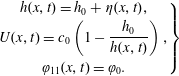 $$\begin{eqnarray}\left.\begin{array}{@{}c@{}}\displaystyle h(x,t)=h_{0}+\unicode[STIX]{x1D702}(x,t),\\ \displaystyle U(x,t)=c_{0}\left(1-\frac{h_{0}}{h(x,t)}\right),\\ \unicode[STIX]{x1D711}_{11}(x,t)=\unicode[STIX]{x1D711}_{0}.\end{array}\right\}\end{eqnarray}$$
The computational domain consists of a
 $200~\text{m}$
long rectangular channel, meshed with a regular triangulation of characteristic size
 $\unicode[STIX]{x0394}x=\unicode[STIX]{x0394}y=0.25~\text{m}$
(see figure 2). The solitary wave is initially located at
 $x_{0}=50~\text{m}$
. We set
 $h_{0}=1~\text{m}$
and impose
 $Fr=1.2$
,
 $\unicode[STIX]{x1D711}_{0}=0.2~\text{s}^{-2}$
, leading to an amplitude
 $a=0.128~\text{m}$
and the initial condition depicted in figure 3. As highlighted by Kazakova & Richard (Reference Kazakova and Richard2019), this gives a solution with a smaller amplitude than the classical solitary wave solution of the Green–Naghdi equations obtained with the same Froude number. We can observe in figure 4 a comparison between analytical and numerical results at several propagation times, obtained with the third-order scheme, highlighting a very good resolution of the wave propagation. Note that the preservation of the initial enstrophy
 $\unicode[STIX]{x1D711}_{0}$
has been numerically confirmed throughout the computation up to the machine error, independently from the mesh size or the polynomial degree in the approximation space.
Test 1: 2-D view of the initial condition.
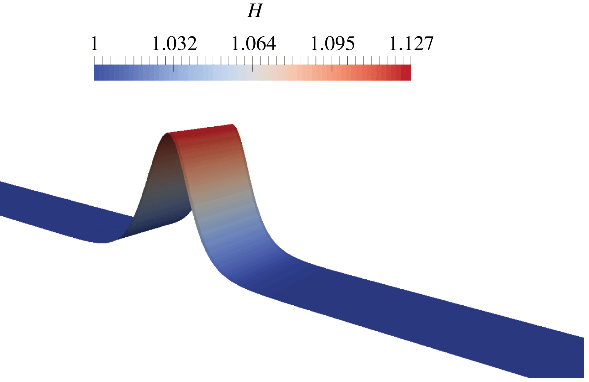
Test 1: 1-D free surface profiles at
 $t=0$
,
 $t=10.25~\text{s}$
,
 $t=20.5~\text{s}$
and
 $t=30.75~\text{s}$
. Exact solution (dots) versus numerical solution (solid curves).
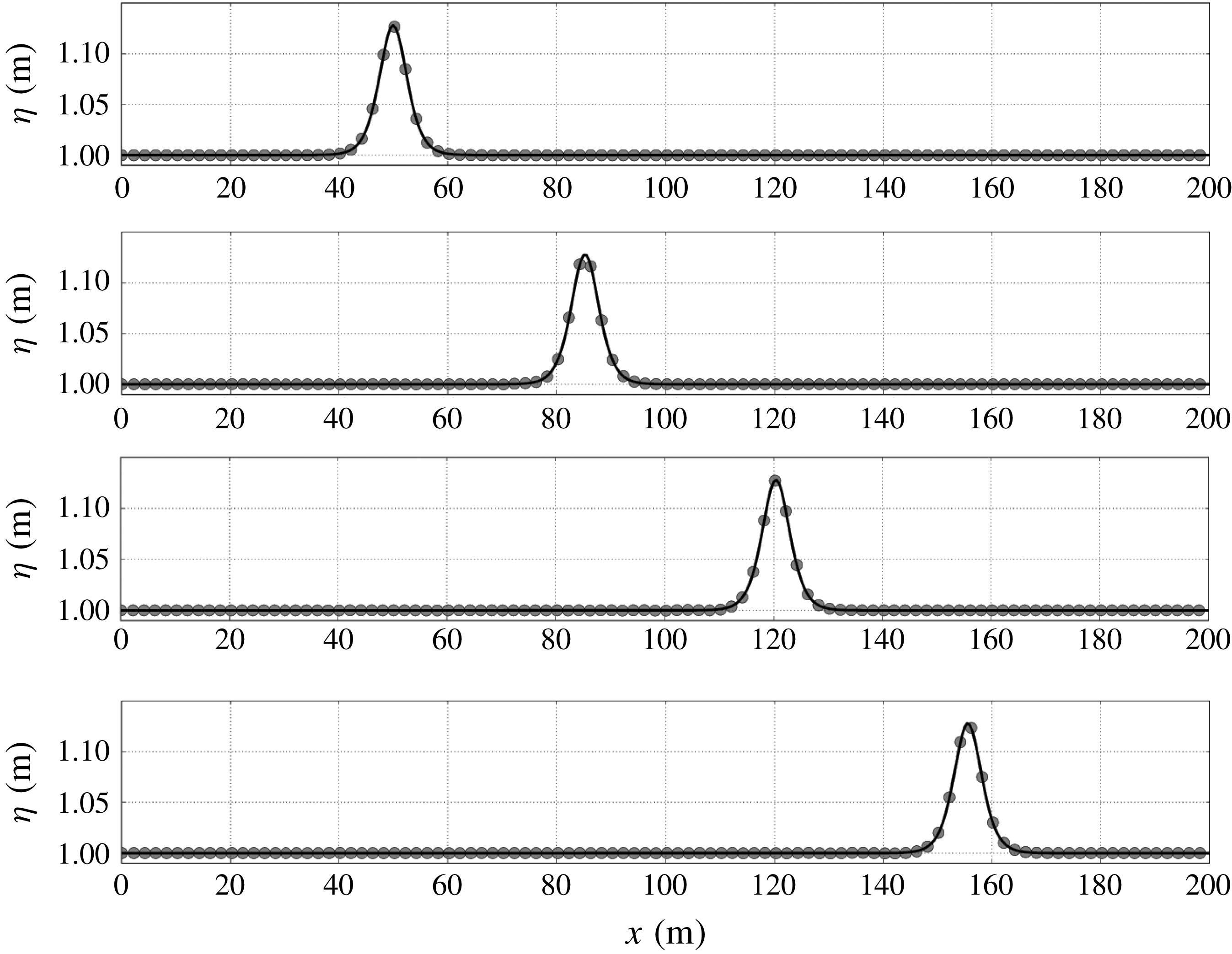
6.2 Wave breaking and run-up of a solitary wave
We now turn to a classical 1-D test case implying wave breaking and run-up, based on the experiment of Synolakis (Reference Synolakis1987). The initial condition consists of an incident wave, obtained as an exact solution of the classical Green–Naghdi equations, propagating over a beach with a constant bed slope
 $s=1/19.85$
. This benchmark is widely used to exhibit the ability to capture shoaling and breaking processes, with subsequent run-up and run-down phenomena (see Zelt Reference Zelt1991; Titov & Synolakis Reference Titov and Synolakis1995; Cienfuegos, Barthelemy & Bonneton Reference Cienfuegos, Barthelemy and Bonneton2010; Tonelli & Petti Reference Tonelli and Petti2010; Bonneton et al.
Reference Bonneton, Chazel, Lannes, Marche and Tissier2011; Tissier et al.
Reference Tissier, Bonneton, Marche, Chazel and Lannes2012; Kazolea, Delis & Synolakis Reference Kazolea, Delis and Synolakis2014, for instance). The numerical set-up implies a solution centred at
 $x_{0}=10~\text{m}$
in a
 $35~\text{m}$
long domain, regularly meshed with a space step
 $\unicode[STIX]{x0394}x=\unicode[STIX]{x0394}y=0.0625~\text{m}$
, as indicated in figure 2. A
 $5~\text{m}$
long sponge layer has been added at the left boundary to stabilize the initiation of the wave propagation. Following the experiment, the reference depth is
 $h_{0}^{\ast }=0.3~\text{m}$
and we consider a relative amplitude
 $a/h_{0}^{\ast }=0.28$
. The topography is given by:
 $$\begin{eqnarray}b(x)=\left\{\begin{array}{@{}ll@{}}\displaystyle 0 & \text{if }x\leqslant 15~\text{m}\\ s(x-15) & \text{otherwise}.\end{array}\right.\end{eqnarray}$$
The laws (5.1) and (5.2) are used for the trigger threshold
 $\unicode[STIX]{x1D713}_{0}$
of the virtual enstrophy and the dimensionless Reynolds number, leading to the values
 $\unicode[STIX]{x1D713}_{0}\approx 6.89~\text{s}^{-2}$
and
 $R\approx 3.87$
in the present case. As stated in § 5, the parameter
 $C_{r}$
has always the constant value
 $C_{r}=0.48$
.
Test 2: comparison of the 1-D free surface profiles between numerical results (solid curves) and experimental data from Synolakis (Reference Synolakis1987) (crosses) at several times during the propagation (
 $t^{\ast }=t(g/h_{0})^{1/2}$
).
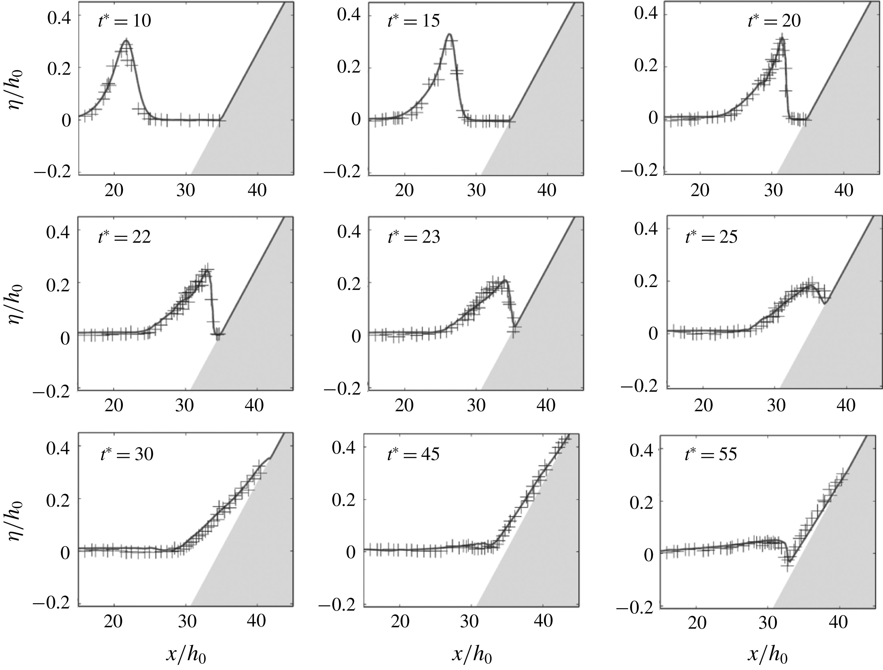
Test 2: virtual enstrophy profile at several times around the breaking point. Wave breaking is identified at
 $t^{\ast }=18.1$
,
 $x=30.3~\text{m}$
.
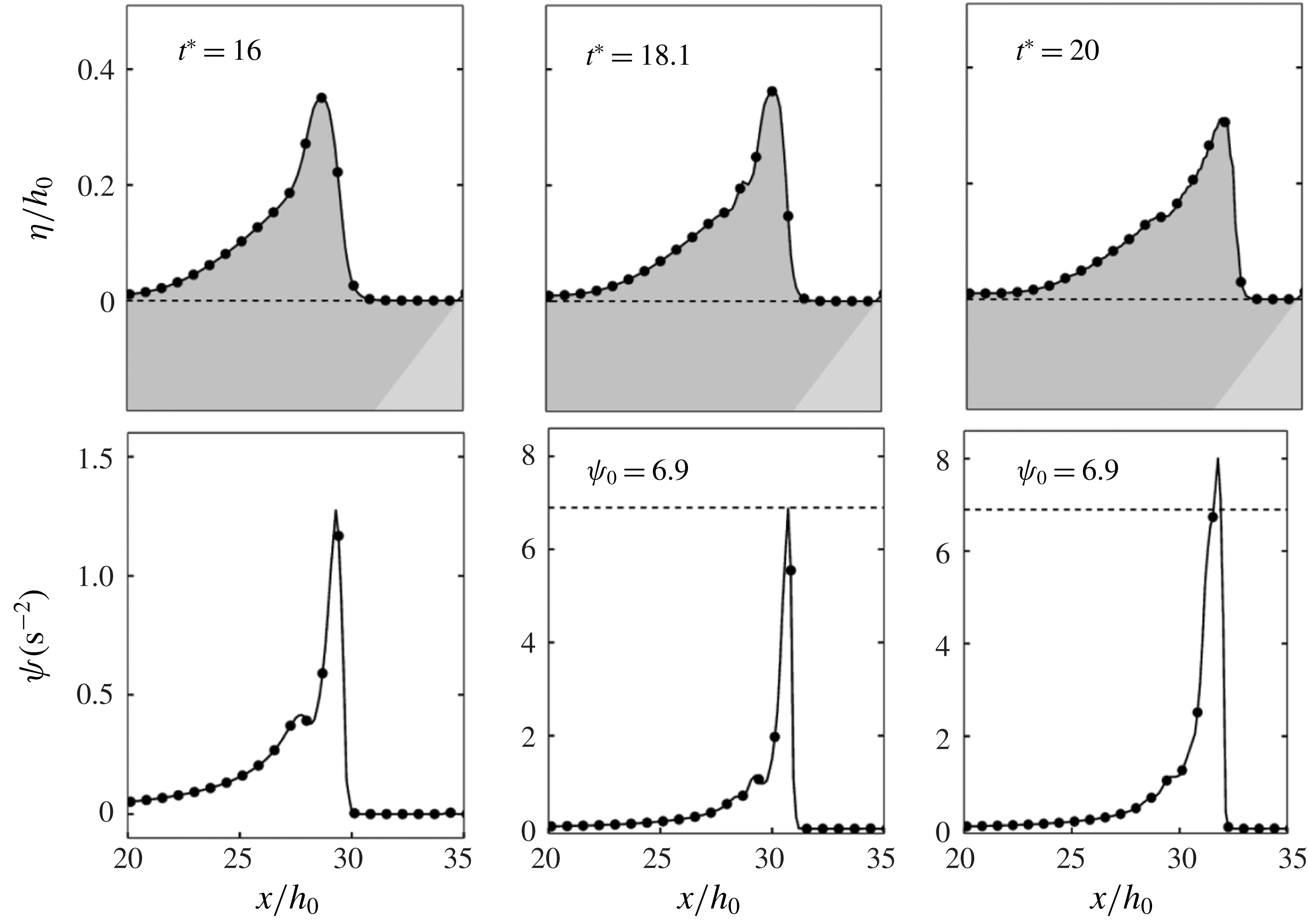
Test 2: virtual enstrophy profile at several times around the second breaking point (hydraulic jump). Wave breaking is identified at
 $t^{\ast }=53$
,
 $x=33.5~\text{m}$
.
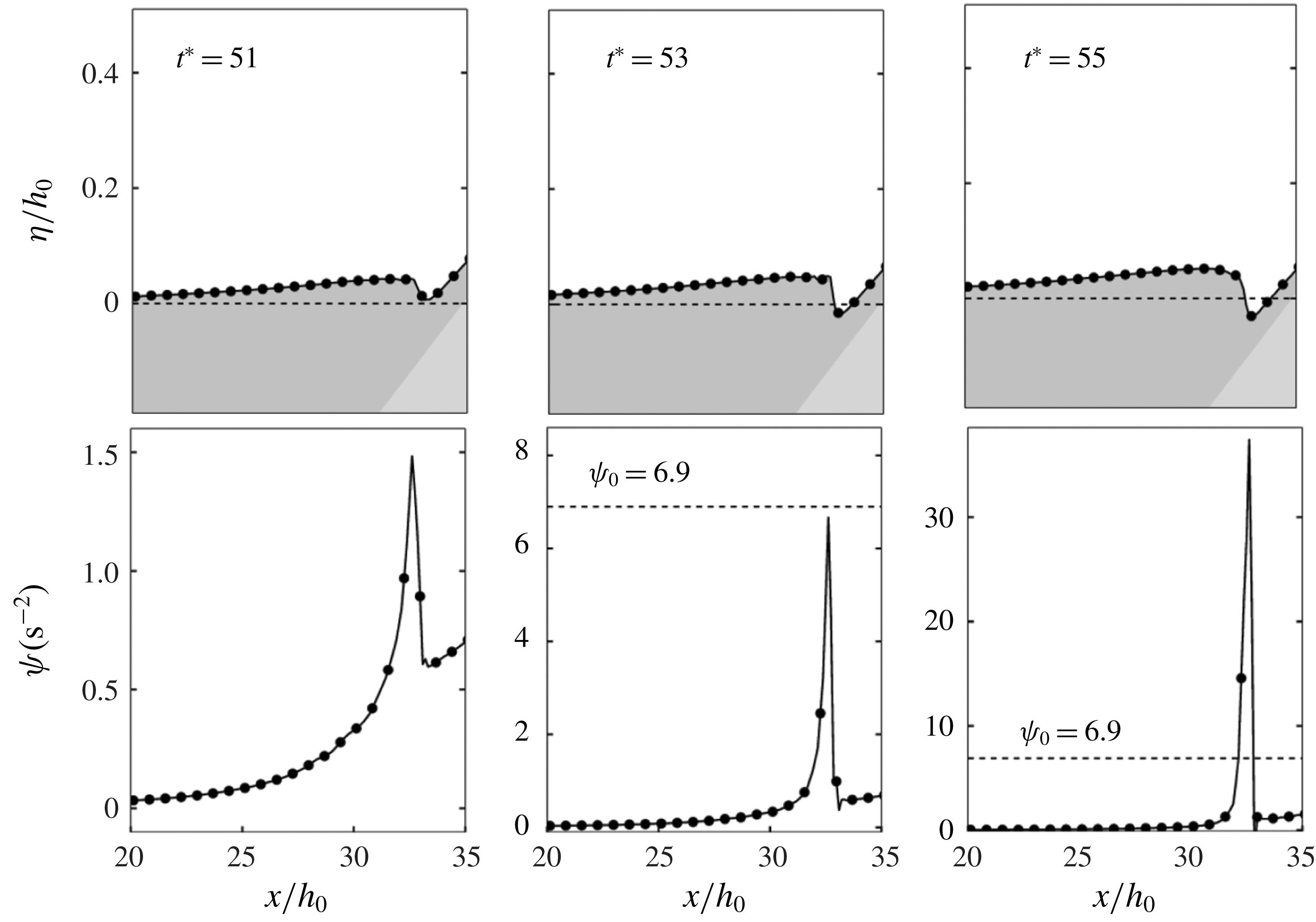
We can observe in figure 5 a comparison between experimental and numerical results at several reference times during the propagation. In accordance with the experimental observations, the wave propagates, shoals and steepens when reaching the shore, as can be seen at times
 $t^{\ast }=t(g/h_{0})^{1/2}=10$
and
 $t^{\ast }=15$
. Then nonlinear effects induced by the bed elevation trigger the breaking of the wave, occurring between
 $t^{\ast }=15$
and
 $t^{\ast }=20$
. To better understand the key role played by the enstrophy variables, a particular focus of the process is available in figure 6. We can see that a sudden production of enstrophy occurs at
 $t^{\ast }=18.1$
, allowing a precise identification of the transition to the turbulent regime. Once the wave is identified as breaking, the enstrophy production is able to correctly balance the dispersive effects and we recover the expected characteristics of the wave transformation, until the end of the run-up phenomenon. Note that since the enstrophy naturally follows the wave motion, there is no need to artificially turn off irrelevant terms or introduce additional de-breaking criteria in regions which are not of concern, as is can be the case with other existing approaches. As reported by Synolakis (Reference Synolakis1987) (see also Kazolea et al.
Reference Kazolea, Delis and Synolakis2014), a second breaking process happens at the end of the computation, in the form of a hydraulic jump around
 $t^{\ast }=53$
. As shown in figure 7, the process in also well captured by the proposed method without any breaking criterion, highlighting the enstrophy as a relevant diagnostic quantity with respect to the general detection of shock waves. These results were obtained with the third-order scheme; identical space and time locations have been observed for the breaking points using other space orders and/or different mesh resolutions. This low sensitivity with respect to the discretization parameters is not surprising, since the breaking criterion is somehow directly resolved as a model variable. Note finally that if a precise and predictive calibration of the breaking parameters
 $(\unicode[STIX]{x1D713}_{0},R)$
has been extracted from the works of Kazakova & Richard (Reference Kazakova and Richard2019), no significant variability has been observed around the corresponding reference values, which also attests to the robustness of the proposed strategy.
These results can be compared to existing models. In switching models the fronts of breaking waves are too steep because these waves are treated as discontinuities and the amplitude is not always correct. This is especially clear at
 $t^{\ast }=20$
(compare our result in figure 5 at
 $t^{\ast }=20$
with the results of Tissier et al. (Reference Tissier, Bonneton, Marche, Chazel and Lannes2012), Kazolea et al. (Reference Kazolea, Delis and Synolakis2014) and Kazolea & Ricchiuto (Reference Kazolea and Ricchiuto2018) at the same time). Moreover all switching models produce spurious oscillations when the mesh size is refined, which prevents numerical convergence.
Eddy-viscosity models behave better than switching models, especially if the turbulent viscosity is calculated with a turbulent kinetic energy for which an equation is solved (Kazolea & Ricchiuto Reference Kazolea and Ricchiuto2018). Our result just after breaking, at
 $t^{\ast }=20$
, is nevertheless slightly better (compare with Roeber, Cheung & Kobayashi Reference Roeber, Cheung and Kobayashi2010; Kazolea et al.
Reference Kazolea, Delis and Synolakis2014 and even Kazolea & Ricchiuto (Reference Kazolea and Ricchiuto2018), all of them having very good results on the whole but a slight discrepancy at the front of this breaking wave). The eddy-viscosity models can have difficulty in detecting the second breaking where a hydraulic jump is created (Kennedy et al.
Reference Kennedy, Chen, Kirby and Dalrymple2000; Kazolea et al.
Reference Kazolea, Delis and Synolakis2014). In any case, a breaking criterion is needed for the initiation of both the first and second breaking events and for the breaking termination.
In our model the profile of the breaking wave is found with a greater accuracy, especially in the front region, and there is no need for a breaking criterion either for the breaking termination or for the initiation of the second breaking. The hydraulic jump is predicted naturally by the model. All these improvements are due to the addition of the enstrophy. This new variable is already known to improve the description of roll waves and turbulent hydraulic jumps (Richard & Gavrilyuk Reference Richard and Gavrilyuk2012, Reference Richard and Gavrilyuk2013) and these new results show that this gives not only a greater accuracy to the simulation of turbulent breaking waves but also more numerical simplicity and robustness by removing the need for some breaking criteria.
6.3 Wave train breaking over a bar
We now turn to a classical test based on the laboratory experiments carried out by Beji & Battjes (Reference Beji and Battjes1993), devoted to the study of periodic sinusoidal waves propagating over a submerged bar. The experimental set-up implies a
 $37.7~\text{m}$
long wave flume equipped with a trapezoidal bar with
 $1/20$
front and
 $1/10$
back slopes, separated by a
 $2~\text{m}$
plane area, leading to the configuration displayed in figure 8. The evolution of the flow is followed at eight wave gauges disposed along the channel, for which experimental data are available. The first one is placed at
 $x=6~\text{m}$
while the others are located at the level of the bar, regularly spaced from
 $x=11$
to
 $x=17~\text{m}$
, as indicated in figure 8. The water depth at rest was set to
 $h_{0}^{\ast }=0.4~\text{m}$
, leading to a
 $0.1~\text{m}$
water depth at the top of the bar.
Test 3: sketch of the experimental configuration of Beji & Battjes (Reference Beji and Battjes1993) and location of the wave gauges.
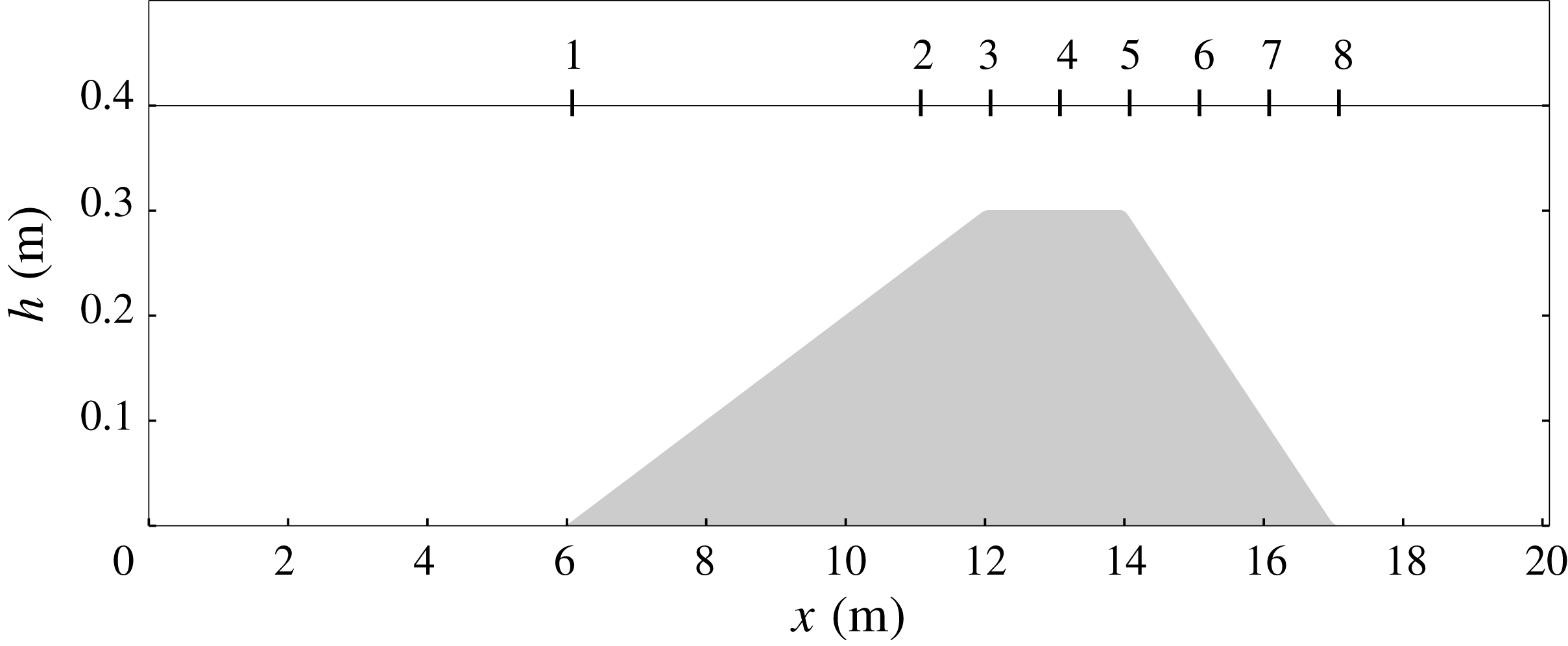
Several series of experiments were run by Beji & Battjes (Reference Beji and Battjes1993), with varying amplitudes and frequencies. The objective pursued here is to show that the current approach can also be applied to capture a complete breaking process in the context of wave trains. This leads us to consider the experimental dataset obtained with a frequency of
 $0.4~\text{Hz}$
and a wave amplitude
 $0.054~\text{m}$
, corresponding to a strongly nonlinear case. In this context, the shoaling of incoming waves is followed by a spilling-type breaking at the arrival at the flat part of the bar. After passing the bar, under the combined effect of the topography and their reintroduction in deeper waters, waves experience highly nonlinear deformations, accompanied by the development of high-order harmonics, close to the dispersive limits of the model. This induces a non-trivial coupling between turbulent effects and highly nonlinear deformations throughout the simulation. Capturing this complex dynamics is therefore a quite challenging issue, generally considered as an important step in the validation of numerical methods for breaking.
Computations have been run on the domain
 $[-10~\text{m},40~\text{m}]$
, including
 $10~\text{m}$
left and right sponge layers to generate incoming waves and to allow for a proper exit of the outgoing waves. A regular mesh with
 $1200$
elements in the
 $x$
-direction was used for this test. As explained in § 5, the initial nonlinearity is small enough to set the activation criterion
 $\unicode[STIX]{x1D713}_{0}$
to zero, meaning that there is no breaking criterion and that the enstrophy is computed everywhere from the beginning of the computation. In this case
 $R$
can be chosen in the interval
 $5<R<10$
(see § 5) and we chose
 $R=7.5$
. As previously discussed, the dissipation parameter
 $C_{r}$
is always equal to
 $0.48$
.
Test 3: free surface (a) and enstrophy (b) profiles at three consecutive times during the breaking process.
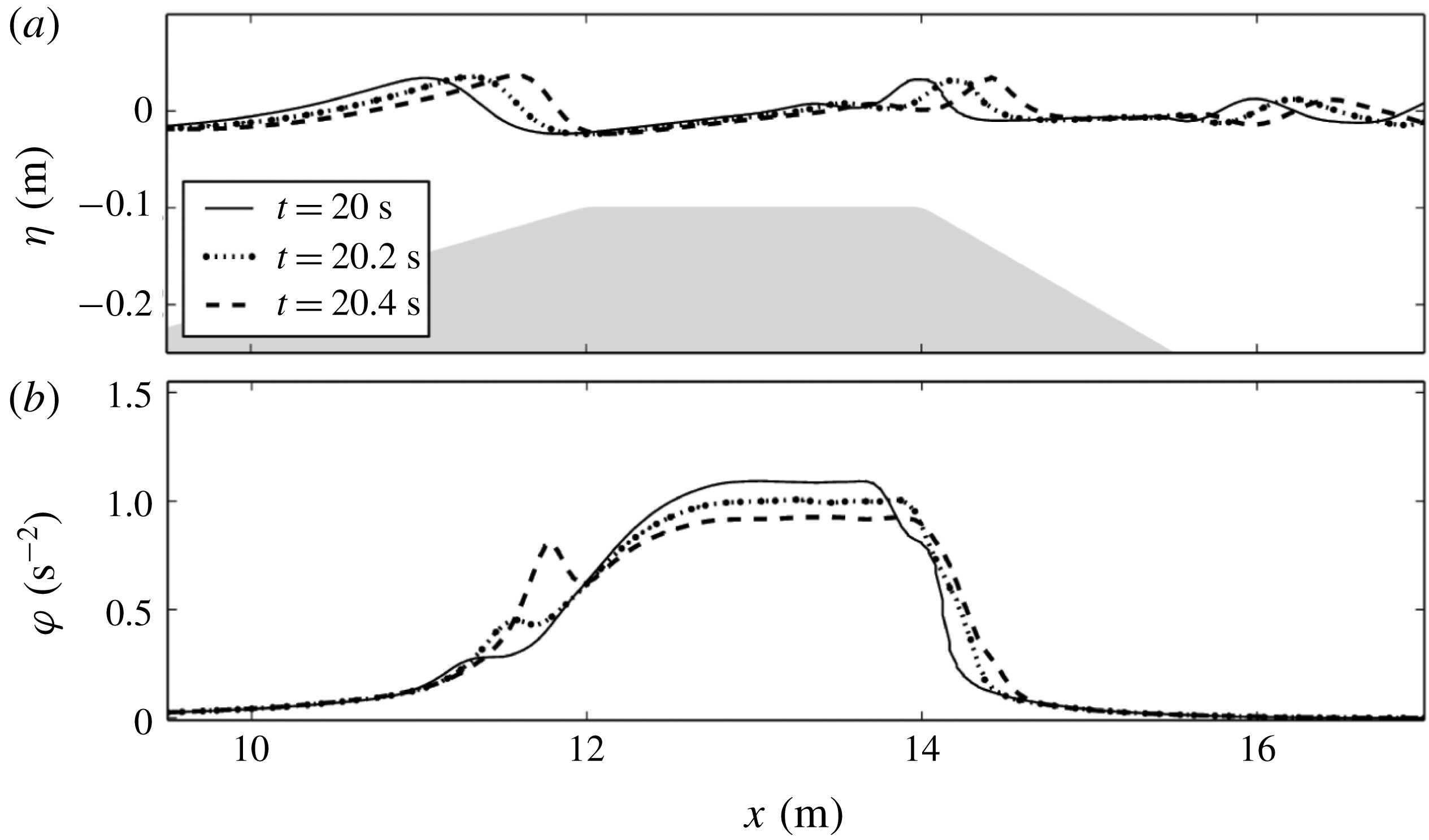
The appearance of enstrophy and its subsequent disappearance (see figure 9) denote the initiation and termination respectively of wave breaking. It is noteworthy that the turbulent effects are not totally damped between two successive waves leading to an accumulation of enstrophy at the level of the bar. These numerical observations are physically relevant, since they highlight that the turbulence produced by a single wave can have not entirely disappeared at the arrival of the following wave, as has been reported in several works (see for instance Ting & Kirby Reference Ting and Kirby1994).
In any case, this accumulation phenomenon is limited in practice and does not break the stability of the method. Further, as shown in figure 10, the method offers a good agreement with the experiments, significantly better than the agreement obtained with usual methods.
Test 3: time series of the free surface elevation at wave gauges. Comparison between the numerical results (curve) and the experimental data of Beji & Battjes (Reference Beji and Battjes1993) (circles).
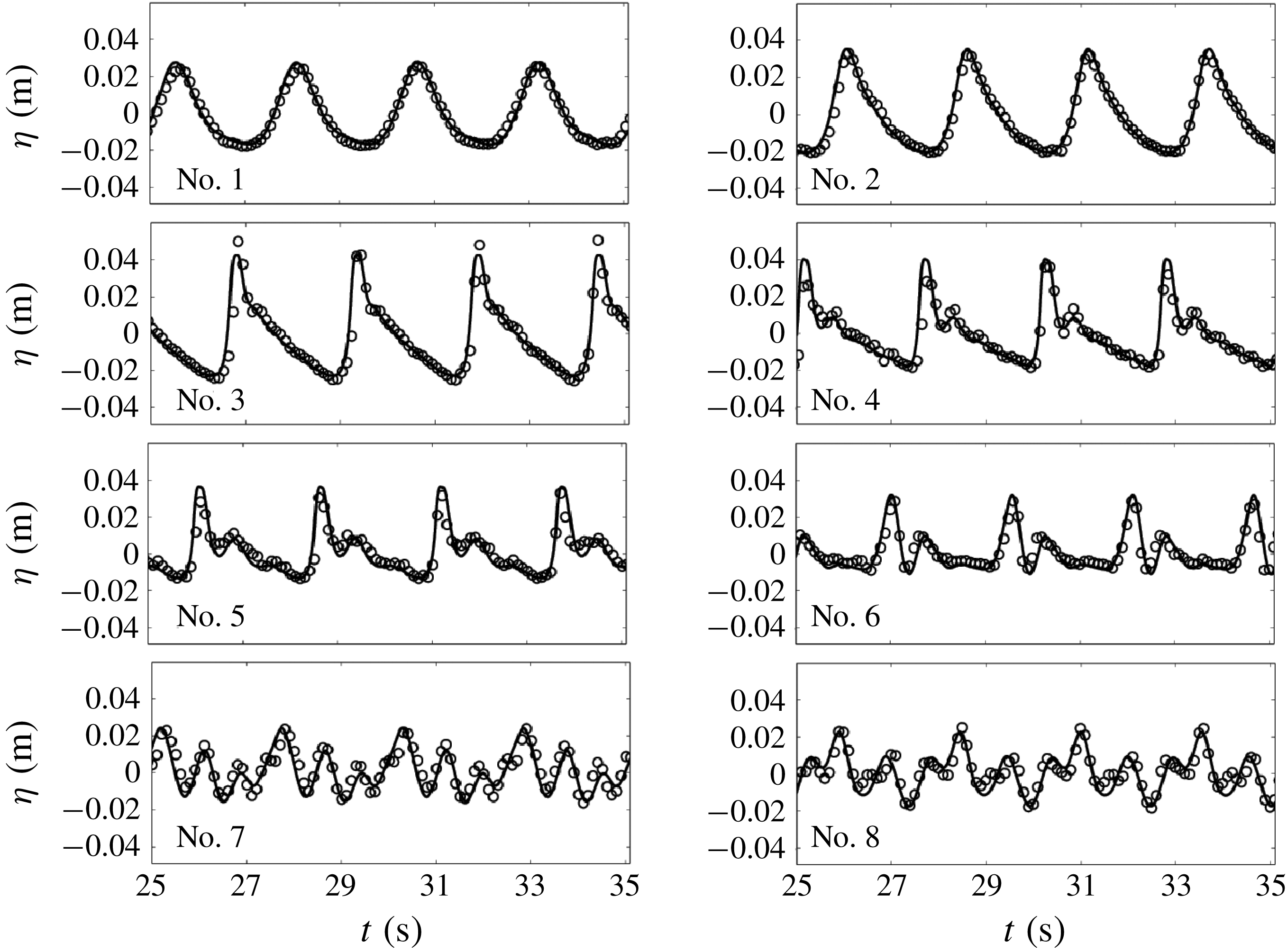
Looking at figure 10 more closely, the results at gauge 2 show that the shoaling process is well described. In particular, we recover the correct amplitudes, while small overestimations can be observed with hybrid methods (see Duran & Marche Reference Duran and Marche2017; Tissier et al. Reference Tissier, Bonneton, Marche, Chazel and Lannes2012), presumably caused by numerical instabilities propagating in the neighbourhood of the breaking area (see also Kazolea & Ricchiuto Reference Kazolea and Ricchiuto2018). Wave breaking occurs at the level of gauge 3. Our results reflect the ability to capture accurately the breaking process, with a precision similar to recent hybrid strategies (Kazolea et al. Reference Kazolea, Delis and Synolakis2014; Filippini et al. Reference Filippini, Kazolea and Ricchiuto2016) but without breaking criterion. Gauges 4 and 5 allow us to examine the continuity of the breaking process. We observe an almost perfect reproduction of the wave transformation, including the free surface inflection at the rear side of the waves, which is not well captured by the models mentioned above (compare the results at gauge 4 in figure 10 with the results at the same gauge in Kazolea & Ricchiuto Reference Kazolea and Ricchiuto2018, figure 6, where it is numbered gauge 3). This improvement in the accuracy of the description of breaking waves compared to eddy-viscosity models is attributable to a better modelling of turbulence through the resolution of the large-scale turbulence with the variable enstrophy. The passing at gauge 6 marks the end of the breaking process, and is accompanied by a more pronounced manifestation of the wave decomposition into secondary waves. To our knowledge, no depth-averaged model is able to provide such a level of agreement at this gauge. As can be seen through gauges 7 and 8, the model is also able to faithfully describe the end of the process, more successfully than the switching strategies (Tissier et al. Reference Tissier, Bonneton, Marche, Chazel and Lannes2012; Duran & Marche Reference Duran and Marche2017), or ad hoc viscosity approaches (Klonaris, Memos & Karambas Reference Klonaris, Memos and Karambas2013). Note finally that the presented results appear to be of the same order of quality as those obtained with direct computational fluid dynamics (CFD) simulations with ad hoc eddy viscosity (Kamath et al. Reference Kamath, Bihs, Chella and Arntsen2015).
As for the previous test case, the switching models produce breaking waves with excessively steep fronts and create numerical instabilities when the mesh is refined. The eddy-viscosity models do not have these problems but they need a breaking criterion for the initiation and termination of the breaking processes as with the switching models. That our model does not need any breaking criterion for this test case is an important improvement since these criteria are a serious weakness of coastal waves models. This does not mean that there is no need for an initiation criterion in other cases of wave trains. In this respect, further work is needed to remove completely the need for a breaking criterion. But the fact that, in some cases at least, no criterion is needed at all is an important result which makes the present approach promising.
6.4 Tsunami wave on a conical island
Based on the laboratory experiments of Liu et al. (Reference Liu, Cho, Briggs, Kanoglu and Synolakis1995) and (Briggs et al.
Reference Briggs, Synolakis, Harkins and Green1995), we now investigate the evolution of a solitary wave propagating over a conical island. This test is regularly employed to study run-up processes and related numerical handling of dry cells with rough topographies in a two-dimensional environment (see for instance Chen et al.
Reference Chen, Kirby, Dalrymple, Kennedy and Chawla2000; Lynett, Wu & Liu Reference Lynett, Wu and Liu2002; Ricchiuto & Bollermann Reference Ricchiuto and Bollermann2009; Kazolea et al.
Reference Kazolea, Delis, Nikolos and Synolakis2012; Azerad, Guermond & Popov Reference Azerad, Guermond and Popov2017). The experimental set-up implies a
 $25~\text{m}$
by
 $30~\text{m}$
basin equipped with a wavemaker calibrated for the generation of solitary waves. The topography is defined as follows:
 $$\begin{eqnarray}b(r)=\left\{\begin{array}{@{}ll@{}}\displaystyle \max \left(0.625,0.9-\frac{r}{4}\right) & \text{if }r<3.6\\ 0 & \text{elsewhere},\end{array}\right.\end{eqnarray}$$
 $r$
being the distance in metres from the centre of the island
 $(x_{0},y_{0})=(12.96~\text{m},13.80~\text{m})$
. The initial water depth is
 $h_{0}^{\ast }=0.32~\text{m}$
. The flow evolution can be tracked through a series of gauges covering the experimental domain, measuring the free surface elevation. Several datasets are available, implying different initial amplitudes of the incident wave. Here we chose a relative amplitude of
 $a/h_{0}^{\ast }=0.2$
, corresponding to the most important initial nonlinearity. In this situation, as reported in Titov & Synolakis (Reference Titov and Synolakis1995), wave breaking is observed all around the island. The phenomenon is however not sufficiently pronounced to threaten the numerical stability and is generally neglected in this respect. The objective here is to show that the method is able to capture these small turbulent effects, while highlighting the possible related benefits.
Test 4: 3-D view of the free surface at
 $t=3~\text{s}$
;
 $6~\text{s}$
;
 $9~\text{s}$
;
 $10~\text{s}$
;
 $11.5~\text{s}$
and
 $12.5~\text{s}$
(from left to right and top to bottom).
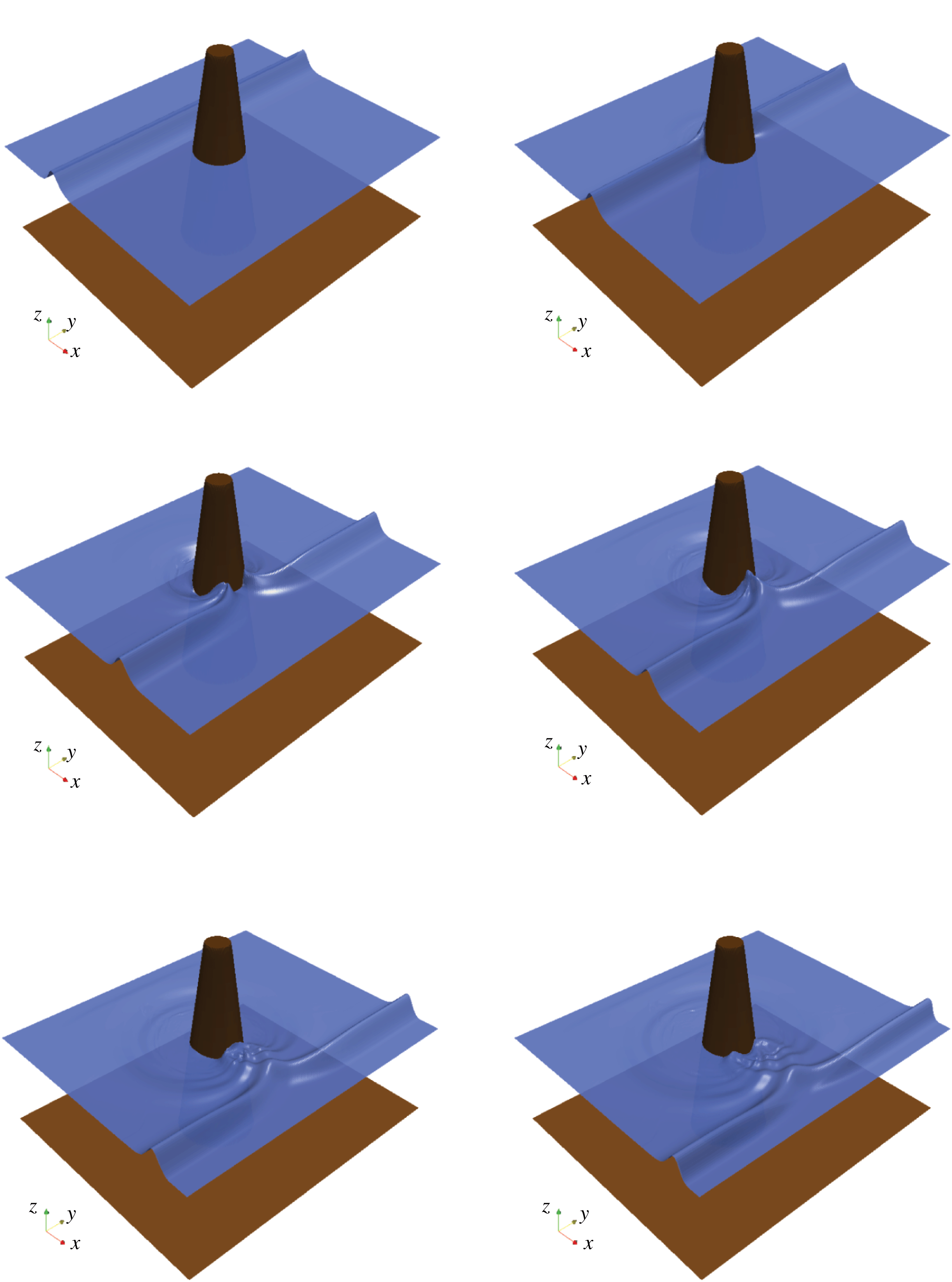
Test 4: positions of the gauges in the experiment of Briggs et al. (Reference Briggs, Synolakis, Harkins and Green1995). The large circle shows the base of the island.
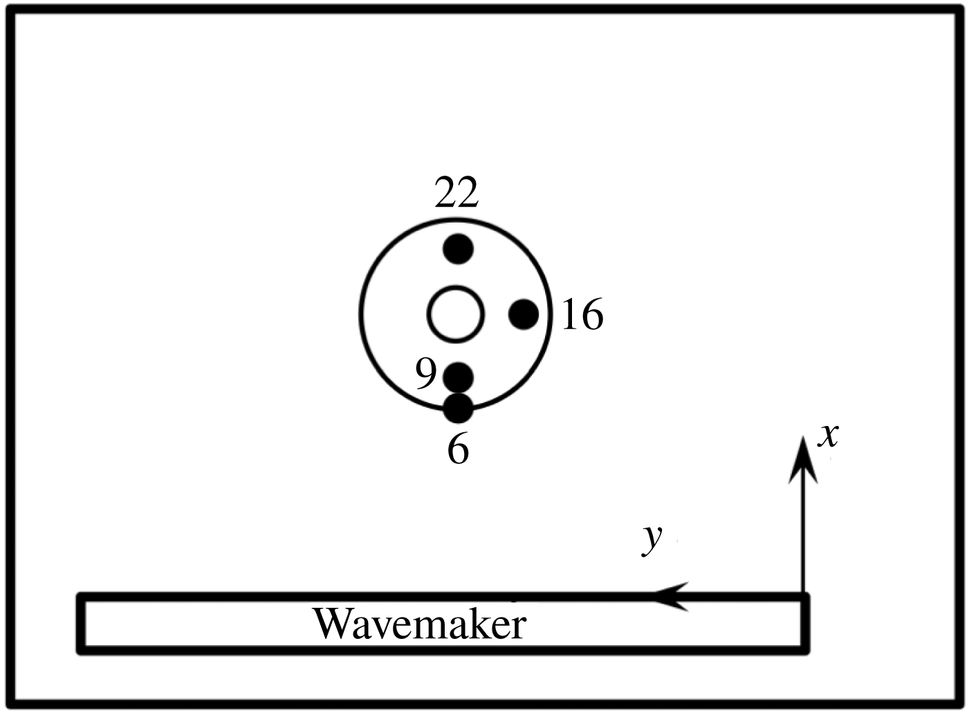
For the numerical simulation we used the third-order scheme on a structured mesh of
 $49\,566$
elements, corresponding to a space step of approximately
 $\unicode[STIX]{x0394}x=\unicode[STIX]{x0394}y=0.167~\text{m}$
. Still based on the law in (5.1), the virtual enstrophy threshold
 $\unicode[STIX]{x1D713}_{0}$
is equal to
 $7.8~\text{s}^{-2}$
. As the dimensionless Reynolds number
 $R$
depends on the topography (5.2), a local strategy can be adopted to calculate the viscosity parameter from the law in (5.2) (i.e.
 $R=0.85$
where
 $s=0$
and
 $R=15.85$
where
 $s=1/4$
). However, we did not observe significant differences using a constant number all over the computational domain corresponding to the average slope (see § 5) and this yields a value of
 $R$
close to 2 (note that there is a weak sensitivity to this value). It is even possible to remove the breaking criterion if
 $s=1/4$
and to take
 $R=0.85$
and
 $\unicode[STIX]{x1D713}_{0}=7.8~\text{s}^{-2}$
if
 $s=0$
and
 $R=7.5$
and
 $\unicode[STIX]{x1D713}_{0}=0$
is
 $s=1/4$
(the two last values being standard when there is no need for a breaking criterion as in § 6.3).
Test 4: time evolution of the free surface at reference gauges.
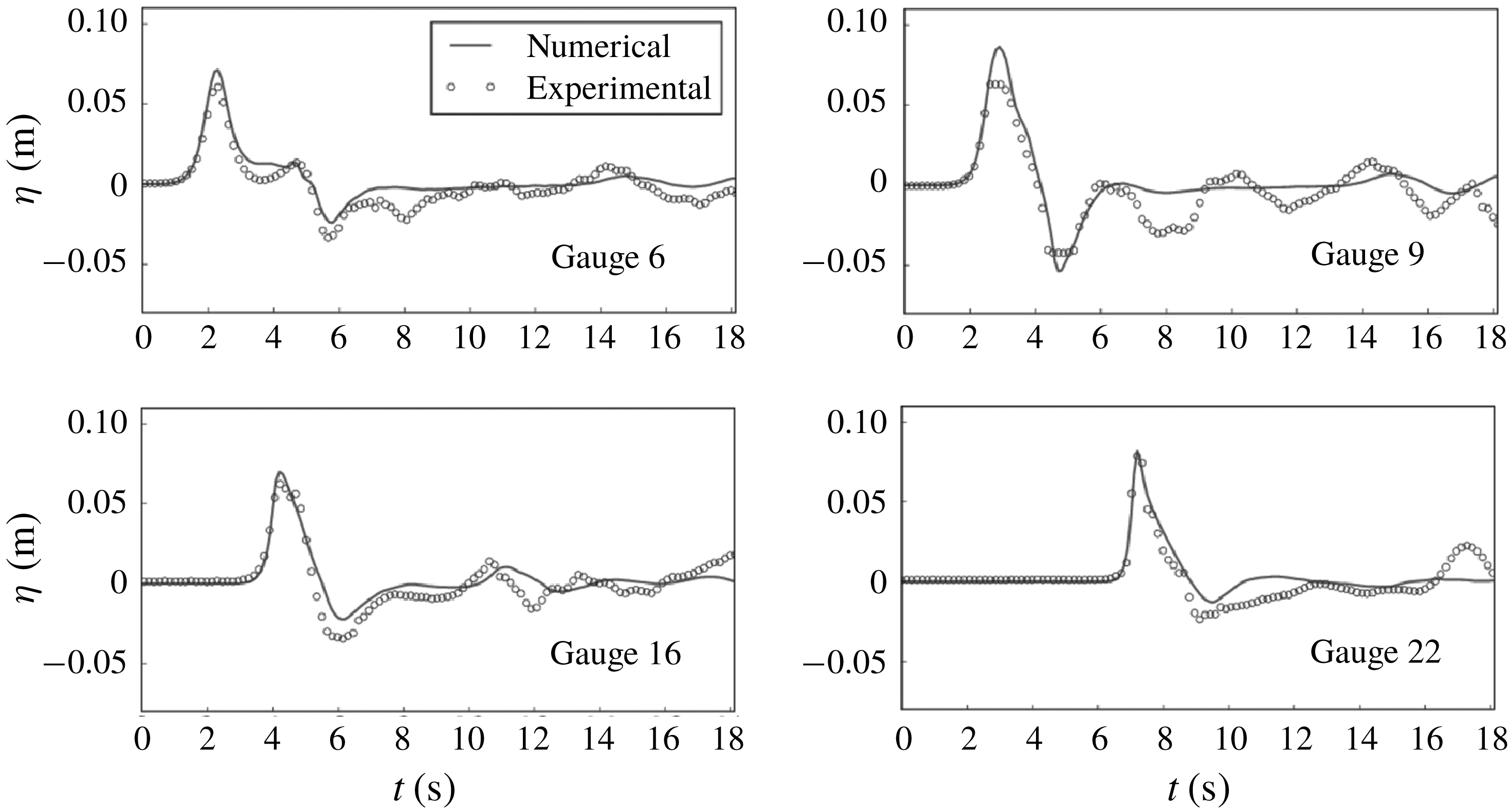
Test 4: time evolution of the trace of the virtual enstrophy tensor at reference gauges.
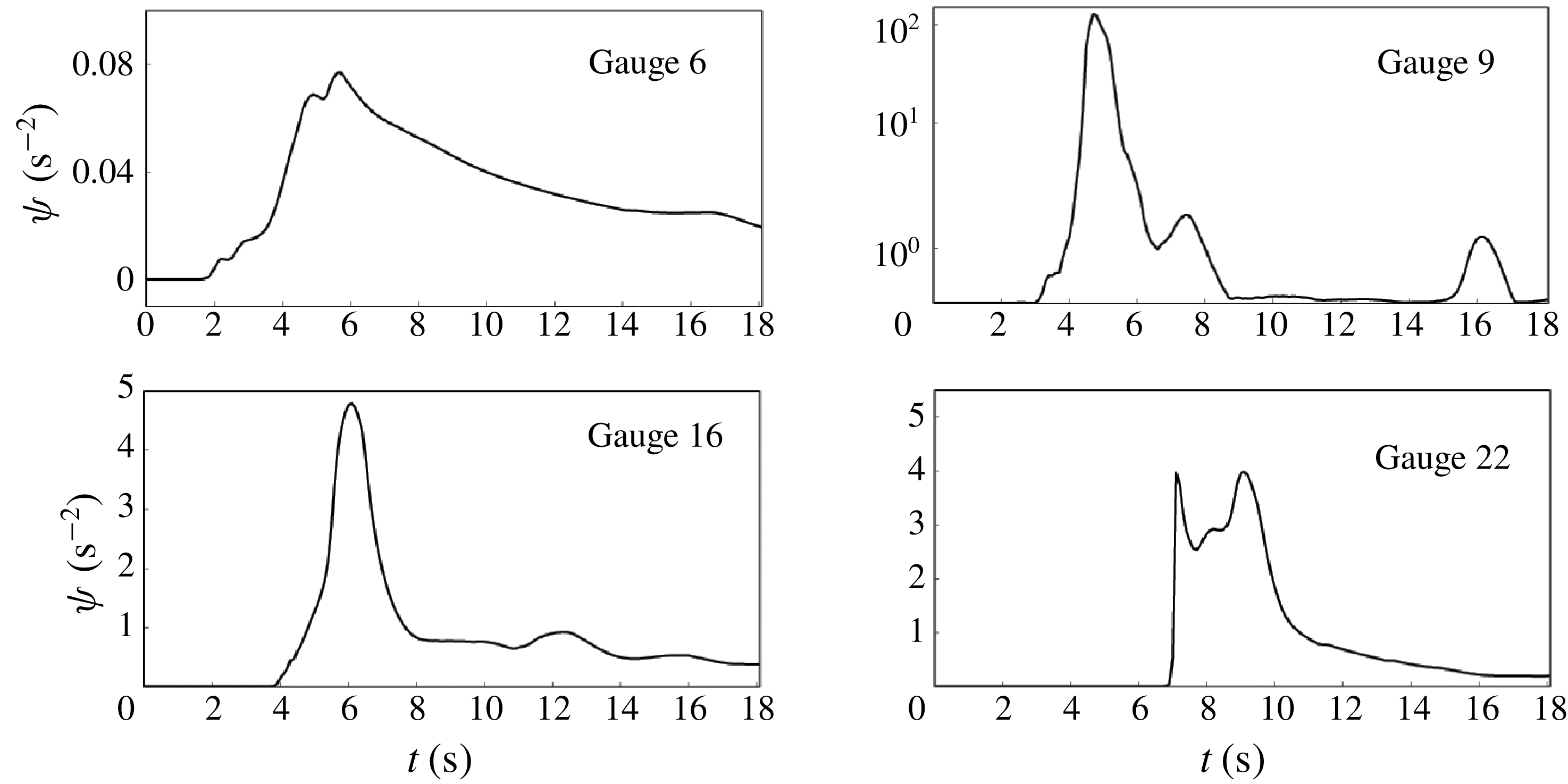
One can observe 3-D snapshots of the solution during the propagation in figure 11, exhibiting a good reproduction of the flow characteristics. In particular, the passing of the emerged part of the island is well resolved, as well as the junction of the two resulting lateral waves at the rear side of the cone and the run-up on the lee side. Time series of the free surface are given at gauge numbers 6, 9, 16 and 22, respectively located at
 $(9.36~\text{m},13.80~\text{m})$
,
 $(10.36~\text{m},13.80~\text{m})$
,
 $(12.96~\text{m},11.22~\text{m})$
and
 $(15.56\,\text{m},13.80\,\text{m})$
. The positions of these gauges are shown in figure 12 and the results are presented in figure 13. We observe a good agreement with the experimental data. In particular, as reported in Kazolea et al. (Reference Kazolea, Delis, Nikolos and Synolakis2012) and Lannes & Marche (Reference Lannes and Marche2015) for instance, slight overestimations of the leading wave amplitude at WG 9 and 22 can be observed when wave breaking is not accounted for (see also Fuhrman & Madsen Reference Fuhrman and Madsen2008). Injecting enstrophy into the system seems to slightly reduce these discrepancies, especially for WG 22 and the minimum run-down amplitude of the reflected wave at WG 9. As confirmed in figure 14, the method is able to identify wave breaking in the vicinity of the island during the passing of the wave. Note that similar results were obtained with a mesh of
 $150\,000$
elements to confirm that these amplitude corrections are not due to under-resolution.
As with all other models, the present model does not capture the small oscillations after the main wave, especially at gauge 9. As discussed by many authors (Kânoǧlu & Synolakis Reference Kânoǧlu and Synolakis1998; Fuhrman & Madsen Reference Fuhrman and Madsen2008; Lannes & Marche Reference Lannes and Marche2015; Zhang et al. Reference Zhang, Kennedy, Tomiczek, Donahue and Westerink2016) the experimental solitary wave profiles were less accurate in their rear part than in their front part and in particular they included a spurious tail which is likely to explain these discrepancies. Additionally, as was pointed out by Liu et al. (Reference Liu, Cho, Briggs, Kanoglu and Synolakis1995), the solitary wave was reflected in the experiments by the boundary of the basin and by the wave generator. This explains some smaller waves which are not captured by the numerical simulations such as the second elevation on the lee side of the island (gauge 22).
6.5 Tsunami wave propagation over a 3-D reef
This last test case is extracted from the laboratory experiments described in Swigler (Reference Swigler2009). The set-up implies the study of a solitary wave evolving within a realistic coastal configuration, including a three-dimensional fringing reef. This is a quite demanding test case, implying highly nonlinear transformations, wave breaking and treatment of shoreline motions in the presence of steep bottom variations. These mechanisms entail complex turbulent dynamics that makes this benchmark in the line of the targeted applications of the proposed model. Recent two-dimensional Boussinesq-type models used this set of data to validate their ability to describe the complexity of surf-zone mechanisms such as wave breaking and bore propagation driven by strongly varying bathymetries (see for instance Roeber & Cheung Reference Roeber and Cheung2012; Shi et al. Reference Shi, Kirby, Harris, Geiman and Grilli2012; Kazolea et al. Reference Kazolea, Delis and Synolakis2014).
Test 5: sketch of the experimental basin with gauges and acoustic Doppler velocimeter (ADV) locations.
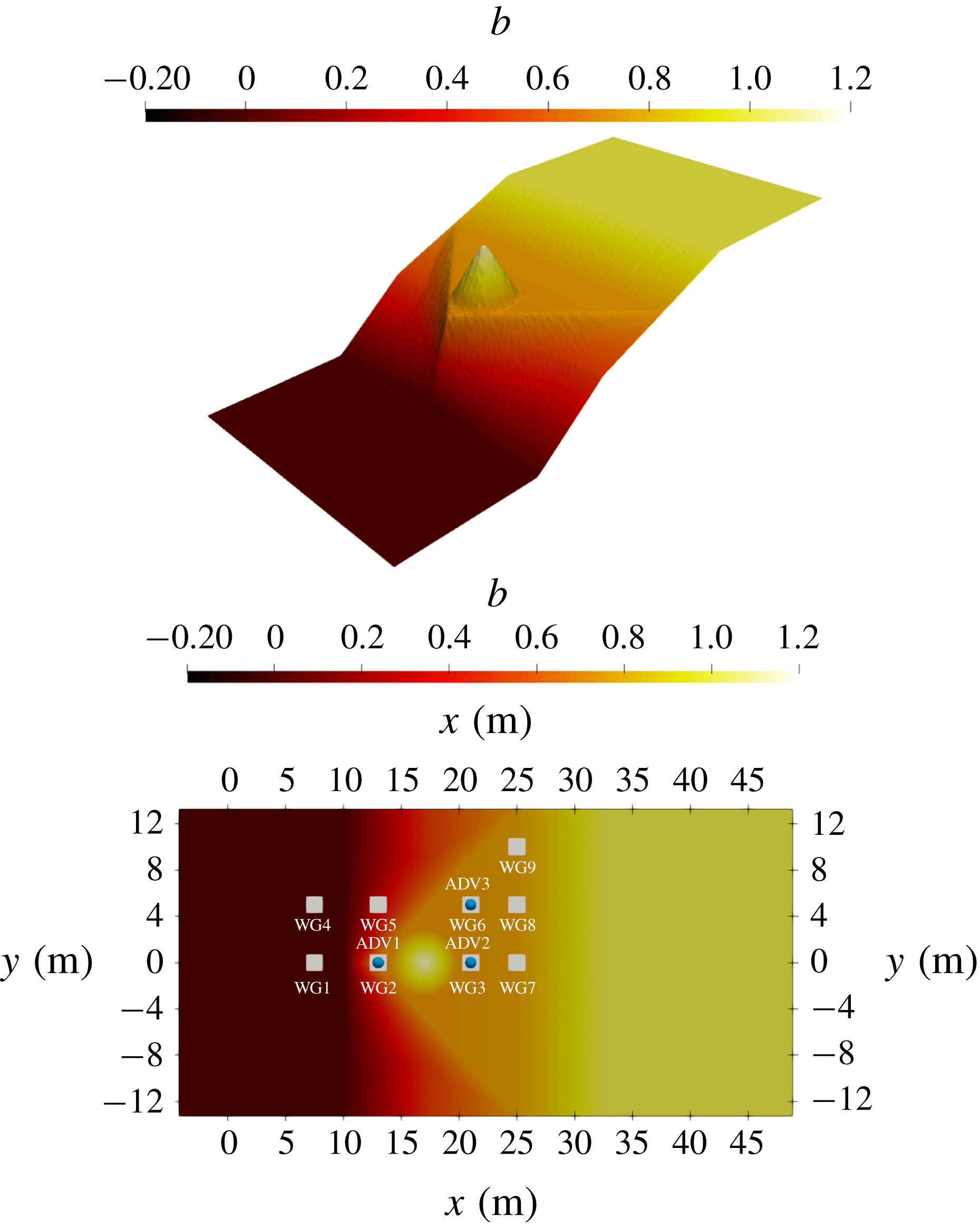
Test 5: snapshots of the free surface during the run-up process. Colour mapping with respect to the quantity
 $\text{tr}\,\unicode[STIX]{x1D753}=\unicode[STIX]{x1D711}_{11}+\unicode[STIX]{x1D711}_{22}$
in
 $\text{s}^{-2}$
.
The experimental basin is
 $48.8~\text{m}$
long and
 $26.5~\text{m}$
wide. The bottom geometry reproduces a planar beach with a triangular flat reef surmounted by an idealized island located at the centre, as can be seen in figure 15. The offshore water depth is set to
 $h_{0}^{\ast }=0.78~\text{m}$
, and the beach slopes extend from
 $x=10$
to
 $x=32.5~\text{m}$
, so that a flat bottom is recovered shortly after the shoreline. The triangular shelf has a maximum elevation of
 $0.71~\text{m}$
and is linearly connected to the beach, with steeper slopes as we get closer to the shelf edge. The island is represented by a
 $6~\text{m}$
diameter cone of
 $0.45~\text{m}$
height centred at
 $x=12.6~\text{m}$
along the
 $y$
-direction centreline. The flow motion is followed by means of a measurement device composed of nine wave gauges, where the free surface was recorded, supplemented by three acoustic Doppler velocimeters (ADVs) to capture the velocity field. Their locations are indicated in table 2 and in figure 15.
Test 5: wave gauges and ADV locations.

The relative amplitude of the incoming wave is
 $a/h_{0}^{\ast }=0.5$
, making this test highly nonlinear. The computational domain was extended at the inlet and outlet boundaries for the generation and the absorption of the solitary wave. The presented results were obtained with the second-order scheme on a mesh of approximatively 200 000 elements, refined in the vicinity of the apex, leading to maximum and minimum areas
 $\max _{T\in {\mathcal{T}}_{h}}\mathfrak{h}_{T}=7.23\times 10^{-2}~\text{m}^{2}$
and
 $\min _{T\in {\mathcal{T}}_{h}}\mathfrak{h}_{T}=6.57\times 10^{-4}~\text{m}^{2}$
respectively. Following the empirical laws (5.1) and (5.2), the breaking threshold is equal to
 $\unicode[STIX]{x1D713}_{0}=2.0~\text{s}^{-2}$
and we set
 $R=3.5$
, which corresponds to an intermediate slope between the maximum and minimum slopes. Naturally, other reasonable choices can be made for this parameter (with a definition depending on the local slopes for instance), but these variations did not have a significant influence on the numerical results.
Figure 16 presents several snapshots of the numerical simulation of the propagation of a solitary wave towards the coast. The colour maps the value of
 $\text{tr}\,\unicode[STIX]{x1D753}$
, which is the turbulent energy of the system times
 $2/h^{2}$
, from deep blue (almost no turbulence) to red (highly turbulent). The red parts correspond to the foamy parts of breaking waves with strong vortices and rollers. Colours refer to the online version of the paper. The movie of this simulation can be found online.
Test 5: time evolution of the surface elevation at reference gauges.
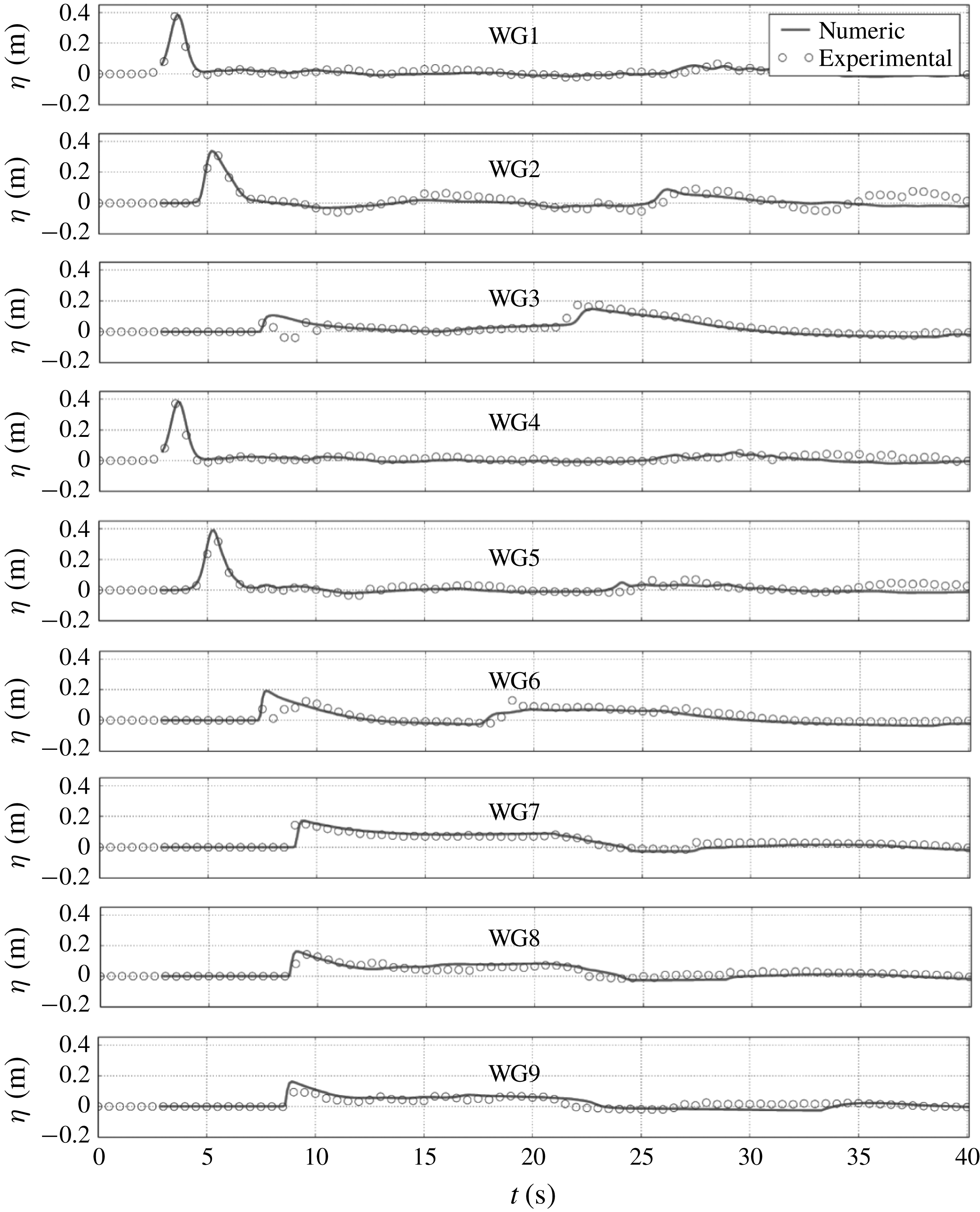
The first important steps of the propagation, corresponding to the passing of the central cone, can be observed in figure 16(a–d). As can be seen through the colour mapping, wave breaking is well captured by the model since the enstrophy is triggered at this stage. In accordance with the experiments and the works mentioned above, we observe a total submersion of the island. The shoaling and breaking processes seem to be well reproduced. In particular, just after the first breaking event at the arrival of the apex, one can see the enstrophy propagating from the centre of the cone to the lateral boundaries, which clearly highlights a progressive transmission of the turbulent structures along the
 $y$
-direction.
Figure 16(e–g) focuses on the termination of the breaking process and the wave propagation over the flat part of the beach. It can be seen that the enstrophy is progressively dissipated, while some residual turbulence can still be observed around the apex. The advancing wave front is well captured, without apparent numerical instabilities.
Figure 16(h–j) proposes snapshots corresponding to the run-down process occurring towards the end of the simulation. Again the scheme is able to detect the formation of a hydraulic jump near the shoreline, which can be seen as the two-dimensional counterpart of what has been observed in one dimension with test 2. Comparisons with experimental data at wave gauges are displayed in figure 17 for the free surface. They exhibit the capability of the model to predict accurately the arrival times of incident and reflected waves and to provide the correct amplitudes throughout the computational domain. Similar observations can be made with the time series of the velocity obtained by ADV proposed in figure 18.
As in the previous cases the switching models tend to produce steeper wave fronts for breaking waves. Again this is explainable by the fact that these models handle breaking waves and turbulent dissipation by a discontinuity. The accuracy of our results is comparable to that of Roeber & Cheung (Reference Roeber and Cheung2012), Shi et al. (Reference Shi, Kirby, Harris, Geiman and Grilli2012) and Kazolea et al. (Reference Kazolea, Delis and Synolakis2014) and there is no phase lag, as is obtained by some models. Moreover due to the superior treatment of the large-scale turbulence, our model is able to remove the need for a breaking criterion both for the breaking termination and for the second breaking initiation during the run-down where a hydraulic jump is formed. A breaking criterion is needed only for the initiation of the first breaking.
Test 5: time evolution of the velocity components at ADVs.
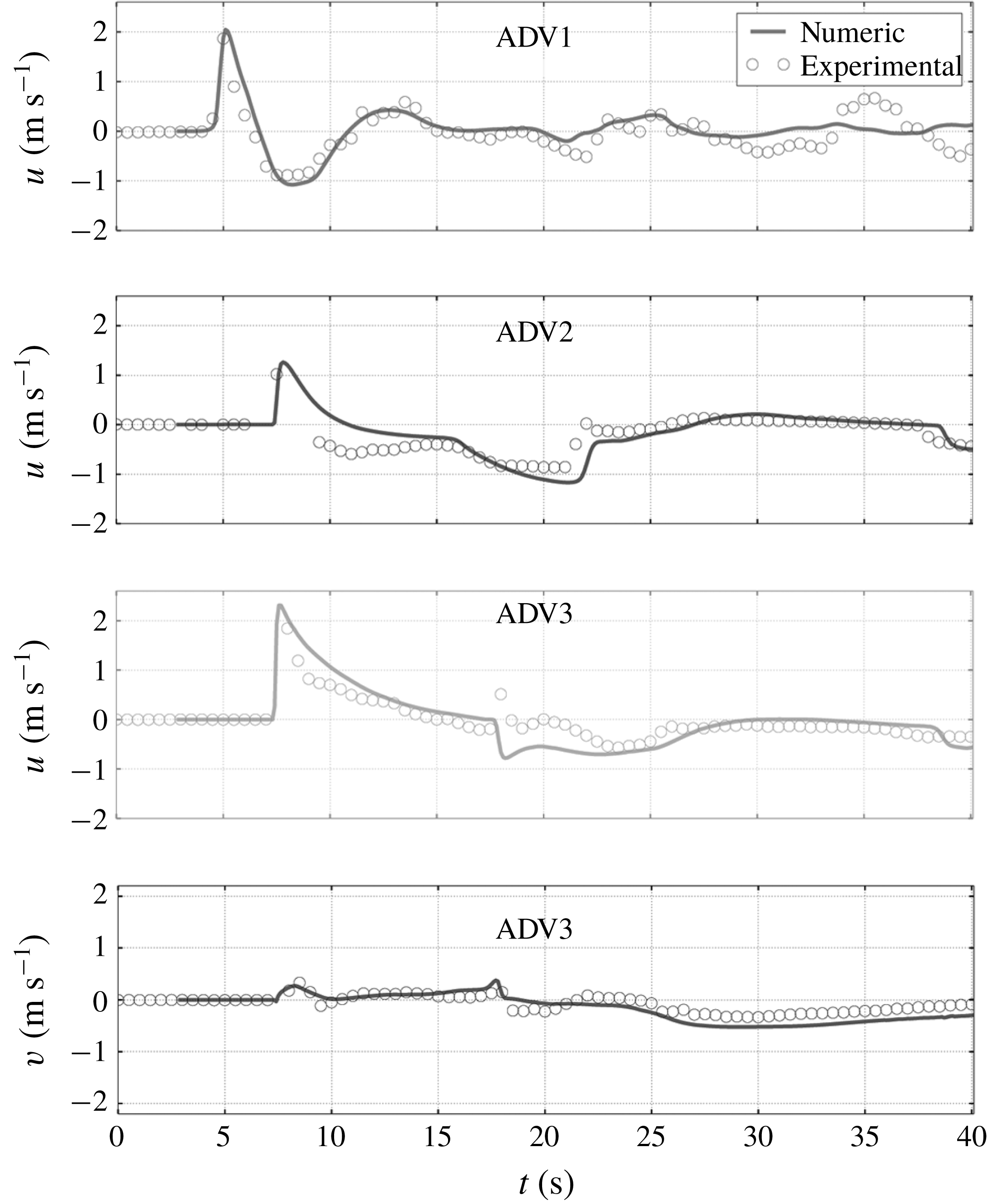
7 Conclusion
We derived a new two-dimensional depth-averaged model for coastal waves under the assumption of a weakly turbulent shallow-water flow. This is an extension of the one-dimensional model of Kazakova & Richard (Reference Kazakova and Richard2019). The subdepth large-scale turbulence is resolved and taken into account by a tensor quantity called enstrophy. This tensor gives an anisotropic character to the model in accordance with the anisotropy of the three-dimensional subdepth large-scale turbulence. This tensor is also a source of vorticity of the mean flow and is responsible for transfers in both directions between the large two-dimensional horizontal eddies with a vertical vorticity and the three-dimensional subdepth turbulence. The small-scale turbulence is modelled with a turbulent-viscosity hypothesis and a depth-uniform eddy viscosity. The weak turbulence assumption is actually equivalent or superior to the hypotheses of other coastal waves models and does not prevent the application of the model to breaking waves in the surf zone with a strong turbulence.
The three equations of the model consist of a scalar equation representing the mass conservation, a vector equation expressing the momentum balance and a tensor equation for the enstrophy tensor. The equation for the trace of this tensor is equivalent to the depth-averaged kinetic energy equation. The eddy viscosity and the turbulent dissipation are obtained by analogy with classical empirical laws. The presence of viscosity and dispersion implies the absence of discontinuities in the solution.
The model is fully nonlinear and its dispersive properties are equivalent to those of the Green–Naghdi equations. These properties were further improved by the method of Bonneton et al. (Reference Bonneton, Chazel, Lannes, Marche and Tissier2011) which can be directly extended to our model. The numerical resolution was obtained by an asymptotically equivalent formulation of the model equations according to the constant diagonal method of Lannes & Marche (Reference Lannes and Marche2015) and by the discontinuous Galerkin scheme of Duran & Marche (Reference Duran and Marche2017). It is noteworthy that the methods developed for the Green–Naghdi equations can be readily adapted to this model since the dispersive terms are identical. The tensor equation includes no dispersive terms nor terms due to the variable bottom. The additional equations are only transport equations with source terms without high-order derivatives, not even of second order. Consequently the numerical resolution complexity is not significantly increased by comparison with the Green–Naghdi equations. Compared to the hybrid or switching methods, there is no problem of mesh grid sensitivity nor of non-physical oscillations.
A breaking criterion is not always needed. When it is needed, the breaking criterion of Kazakova & Richard (Reference Kazakova and Richard2019) for solitary waves can be taken directly as well as the values for the parameters of the model. There is no need for a breaking termination criterion. There is a low sensitivity to the precise values of these parameters and also to the discretization parameters, which gives an appreciable robustness to the model. These improvements are attributable to the presence in the model of a quantity resolving explicitly the large-scale turbulence. The partial removal of the breaking criteria is already an important result. Future works on this approach should endeavour to remove completely these criteria which would be an important improvement in coastal wave modelling.
The model was used to simulate various cases of solitary wave propagation and one case of wave trains. Studied phenomena include the run-up and run-down of a wave over a beach, the propagation of a wave train over a bar and the two-dimensional waves propagation around an island or around a reef and on a sloping beach. The agreement with the experimental measures is very good in all cases. In particular the breaking phenomenon, including the hydraulic jump appearing in a run-down phase, are better or more easily described than in previous depth-averaged models. The numerical simulations show that this new model is numerically robust and that it has a predictive character and a high physical content without significant increase in numerical complexity.
All these results show that this approach is really promising but it should be extended in a future work to a thorough study of wave trains and of the different types of breaking processes, mainly the spilling and plunging types. In particular, the empirical laws for the models parameters, which are well established in the case of a solitary wave, are needed for wave trains in order to give the model a complete predictive character.
Acknowledgements
The work was supported by the Service Hydrographique et Océanographique de la Marine (SHOM). The authors were supported by the French National Research Agency project NABUCO, grant ANR-17-CE40-0025. A.D. and G.L.R. would like to acknowledge financial and scientific support from the French CNRS program PEPS (Projets Exploratoires Premier Soutien).
Supplementary movie
A movie of the numerical simulation of the two-dimensional propagation of a solitary wave around a reef over a sloping beach, including run-up and run-down (test case of § 6.5), is available as an online supplementary material.
Supplementary movie is available at https://doi.org/10.1017/jfm.2019.125.
Appendix A. Conventions used in tensor calculus
For any vector (first-order tensor)
 $\boldsymbol{V}=V_{i}\boldsymbol{e}_{\boldsymbol{i}}$
, second-order tensor
 $\unicode[STIX]{x1D63C}=\unicode[STIX]{x1D608}_{ij}\boldsymbol{e}_{\boldsymbol{i}}\,\otimes \,\boldsymbol{e}_{\boldsymbol{j}}$
and
 $\unicode[STIX]{x1D63C}^{\prime }=\unicode[STIX]{x1D608}_{ij}^{\prime }\boldsymbol{e}_{\boldsymbol{i}}\,\otimes \,\boldsymbol{e}_{\boldsymbol{j}}$
or third-order tensor
 $\unicode[STIX]{x1D63D}=\unicode[STIX]{x1D609}_{ijk}\boldsymbol{e}_{\boldsymbol{i}}\,\otimes \,\boldsymbol{e}_{\boldsymbol{j}}\,\otimes \,\boldsymbol{e}_{\boldsymbol{k}}$
(using Einstein notation), the dot product is defined as
 $$\begin{eqnarray}\unicode[STIX]{x1D63C}\boldsymbol{\cdot }\unicode[STIX]{x1D63C}^{\prime }=\unicode[STIX]{x1D608}_{ik}\unicode[STIX]{x1D608}_{kj}^{\prime }\boldsymbol{e}_{\boldsymbol{ i}}\,\otimes \,\boldsymbol{e}_{\boldsymbol{j}},\end{eqnarray}$$
the double dot product is defined as
 $$\begin{eqnarray}\unicode[STIX]{x1D63C}:\unicode[STIX]{x1D63C}^{\prime }=\unicode[STIX]{x1D608}_{ij}\unicode[STIX]{x1D608}_{ji}^{\prime },\end{eqnarray}$$
the divergence operator is defined as
 $$\begin{eqnarray}\text{div}\,\boldsymbol{U}=\frac{\unicode[STIX]{x2202}U_{i}}{\unicode[STIX]{x2202}x_{i}},\quad \mathbf{div}\,\unicode[STIX]{x1D63C}=\frac{\unicode[STIX]{x2202}\unicode[STIX]{x1D608}_{ij}}{\unicode[STIX]{x2202}x_{j}}\boldsymbol{e}_{\boldsymbol{i}},\quad \unicode[STIX]{x1D5F1}\unicode[STIX]{x1D5F6}\unicode[STIX]{x1D603}\,\unicode[STIX]{x1D63D}=\frac{\unicode[STIX]{x2202}\unicode[STIX]{x1D609}_{ijk}}{\unicode[STIX]{x2202}x_{k}}\boldsymbol{e}_{\boldsymbol{i}}\,\otimes \,\boldsymbol{e}_{\boldsymbol{j}},\end{eqnarray}$$
and the gradient of a vector is defined as
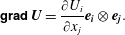 $$\begin{eqnarray}\unicode[STIX]{x1D5F4}\unicode[STIX]{x1D5FF}\unicode[STIX]{x1D5EE}\unicode[STIX]{x1D5F1}\,\boldsymbol{U}=\frac{\unicode[STIX]{x2202}U_{i}}{\unicode[STIX]{x2202}x_{j}}\boldsymbol{e}_{\boldsymbol{i}}\,\otimes \,\boldsymbol{e}_{\boldsymbol{j}}.\end{eqnarray}$$
Appendix B. Equations of the model
The complete system of equations can be written with the components
 $U$
and
 $V$
of the average velocity and with the three independent components
 $\unicode[STIX]{x1D711}_{11}$
,
 $\unicode[STIX]{x1D711}_{12}$
and
 $\unicode[STIX]{x1D711}_{22}$
of the symmetrical enstrophy tensor. The mass equation (2.23) can be written
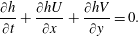 $$\begin{eqnarray}\frac{\unicode[STIX]{x2202}h}{\unicode[STIX]{x2202}t}+\frac{\unicode[STIX]{x2202}hU}{\unicode[STIX]{x2202}x}+\frac{\unicode[STIX]{x2202}hV}{\unicode[STIX]{x2202}y}=0.\end{eqnarray}$$
The momentum equation (2.38) in dimensional form gives the two scalar equations
 $$\begin{eqnarray}\displaystyle & & \displaystyle \frac{\unicode[STIX]{x2202}hU}{\unicode[STIX]{x2202}t}+\frac{\unicode[STIX]{x2202}}{\unicode[STIX]{x2202}x}(hU^{2}+h^{3}\unicode[STIX]{x1D711}_{11}+\unicode[STIX]{x1D6F1}+\unicode[STIX]{x1D6F1}^{\prime })+\frac{\unicode[STIX]{x2202}}{\unicode[STIX]{x2202}y}(hUV+h^{3}\unicode[STIX]{x1D711}_{12})\nonumber\\ \displaystyle & & \displaystyle \quad =-gh\frac{\unicode[STIX]{x2202}b}{\unicode[STIX]{x2202}x}+\frac{\unicode[STIX]{x2202}}{\unicode[STIX]{x2202}x}\left(4\unicode[STIX]{x1D708}_{T}h\frac{\unicode[STIX]{x2202}U}{\unicode[STIX]{x2202}x}+2\unicode[STIX]{x1D708}_{T}h\frac{\unicode[STIX]{x2202}V}{\unicode[STIX]{x2202}y}\right)+\frac{\unicode[STIX]{x2202}}{\unicode[STIX]{x2202}y}\left(\unicode[STIX]{x1D708}_{T}h\frac{\unicode[STIX]{x2202}U}{\unicode[STIX]{x2202}y}+\unicode[STIX]{x1D708}_{T}h\frac{\unicode[STIX]{x2202}V}{\unicode[STIX]{x2202}x}\right)-f_{x}^{\prime },\qquad\end{eqnarray}$$
 $$\begin{eqnarray}\displaystyle & & \displaystyle \frac{\unicode[STIX]{x2202}hV}{\unicode[STIX]{x2202}t}+\frac{\unicode[STIX]{x2202}}{\unicode[STIX]{x2202}x}(hUV+h^{3}\unicode[STIX]{x1D711}_{12})+\frac{\unicode[STIX]{x2202}}{\unicode[STIX]{x2202}y}(hV^{2}+h^{3}\unicode[STIX]{x1D711}_{22}+\unicode[STIX]{x1D6F1}+\unicode[STIX]{x1D6F1}^{\prime })\nonumber\\ \displaystyle & & \displaystyle \quad =-gh\frac{\unicode[STIX]{x2202}b}{\unicode[STIX]{x2202}y}+\frac{\unicode[STIX]{x2202}}{\unicode[STIX]{x2202}x}\left(\unicode[STIX]{x1D708}_{T}h\frac{\unicode[STIX]{x2202}V}{\unicode[STIX]{x2202}x}+\unicode[STIX]{x1D708}_{T}h\frac{\unicode[STIX]{x2202}U}{\unicode[STIX]{x2202}y}\right)+\frac{\unicode[STIX]{x2202}}{\unicode[STIX]{x2202}y}\left(2\unicode[STIX]{x1D708}_{T}h\frac{\unicode[STIX]{x2202}U}{\unicode[STIX]{x2202}x}+4\unicode[STIX]{x1D708}_{T}h\frac{\unicode[STIX]{x2202}V}{\unicode[STIX]{x2202}y}\right)-f_{y}^{\prime }.\qquad\end{eqnarray}$$
The enstrophy equation (2.49) in dimensional form gives the three scalar equations
 $$\begin{eqnarray}\displaystyle & & \displaystyle \frac{\unicode[STIX]{x2202}h\unicode[STIX]{x1D711}_{11}}{\unicode[STIX]{x2202}t}+\frac{\unicode[STIX]{x2202}hU\unicode[STIX]{x1D711}_{11}}{\unicode[STIX]{x2202}x}+\frac{\unicode[STIX]{x2202}hV\unicode[STIX]{x1D711}_{11}}{\unicode[STIX]{x2202}y}=2h\unicode[STIX]{x1D711}_{11}\frac{\unicode[STIX]{x2202}V}{\unicode[STIX]{x2202}y}-2h\unicode[STIX]{x1D711}_{12}\frac{\unicode[STIX]{x2202}U}{\unicode[STIX]{x2202}y}\nonumber\\ \displaystyle & & \displaystyle \quad +\,\frac{\unicode[STIX]{x1D708}_{T}}{h}\left[8\left(\frac{\unicode[STIX]{x2202}U}{\unicode[STIX]{x2202}x}\right)^{2}+4\frac{\unicode[STIX]{x2202}U}{\unicode[STIX]{x2202}x}\frac{\unicode[STIX]{x2202}V}{\unicode[STIX]{x2202}y}+2\frac{\unicode[STIX]{x2202}U}{\unicode[STIX]{x2202}y}\frac{\unicode[STIX]{x2202}V}{\unicode[STIX]{x2202}x}+2\left(\frac{\unicode[STIX]{x2202}U}{\unicode[STIX]{x2202}y}\right)^{2}\right]-C_{r}h\unicode[STIX]{x1D711}_{11}\sqrt{\unicode[STIX]{x1D711}_{11}+\unicode[STIX]{x1D711}_{22}},\qquad\end{eqnarray}$$
 $$\begin{eqnarray}\displaystyle & & \displaystyle \frac{\unicode[STIX]{x2202}h\unicode[STIX]{x1D711}_{12}}{\unicode[STIX]{x2202}t}+\frac{\unicode[STIX]{x2202}hU\unicode[STIX]{x1D711}_{12}}{\unicode[STIX]{x2202}x}+\frac{\unicode[STIX]{x2202}hV\unicode[STIX]{x1D711}_{12}}{\unicode[STIX]{x2202}y}=h\unicode[STIX]{x1D711}_{12}\left(\frac{\unicode[STIX]{x2202}U}{\unicode[STIX]{x2202}x}+\frac{\unicode[STIX]{x2202}V}{\unicode[STIX]{x2202}y}\right)-h\unicode[STIX]{x1D711}_{11}\frac{\unicode[STIX]{x2202}V}{\unicode[STIX]{x2202}x}-h\unicode[STIX]{x1D711}_{22}\frac{\unicode[STIX]{x2202}U}{\unicode[STIX]{x2202}y}\nonumber\\ \displaystyle & & \displaystyle \quad +\,\frac{\unicode[STIX]{x1D708}_{T}}{h}\left[3\left(\frac{\unicode[STIX]{x2202}U}{\unicode[STIX]{x2202}x}\frac{\unicode[STIX]{x2202}U}{\unicode[STIX]{x2202}y}+\frac{\unicode[STIX]{x2202}V}{\unicode[STIX]{x2202}x}\frac{\unicode[STIX]{x2202}V}{\unicode[STIX]{x2202}y}\right)+5\left(\frac{\unicode[STIX]{x2202}U}{\unicode[STIX]{x2202}x}\frac{\unicode[STIX]{x2202}V}{\unicode[STIX]{x2202}x}+\frac{\unicode[STIX]{x2202}U}{\unicode[STIX]{x2202}y}\frac{\unicode[STIX]{x2202}V}{\unicode[STIX]{x2202}y}\right)\right]-C_{r}h\unicode[STIX]{x1D711}_{12}\sqrt{\unicode[STIX]{x1D711}_{11}+\unicode[STIX]{x1D711}_{22}},\nonumber\\ \displaystyle & & \displaystyle\end{eqnarray}$$
and
 $$\begin{eqnarray}\displaystyle & & \displaystyle \frac{\unicode[STIX]{x2202}h\unicode[STIX]{x1D711}_{22}}{\unicode[STIX]{x2202}t}+\frac{\unicode[STIX]{x2202}hU\unicode[STIX]{x1D711}_{22}}{\unicode[STIX]{x2202}x}+\frac{\unicode[STIX]{x2202}hV\unicode[STIX]{x1D711}_{22}}{\unicode[STIX]{x2202}y}=2h\unicode[STIX]{x1D711}_{22}\frac{\unicode[STIX]{x2202}U}{\unicode[STIX]{x2202}x}-2h\unicode[STIX]{x1D711}_{12}\frac{\unicode[STIX]{x2202}V}{\unicode[STIX]{x2202}x}\nonumber\\ \displaystyle & & \displaystyle \quad +\,\frac{\unicode[STIX]{x1D708}_{T}}{h}\left[8\left(\frac{\unicode[STIX]{x2202}V}{\unicode[STIX]{x2202}y}\right)^{2}+4\frac{\unicode[STIX]{x2202}U}{\unicode[STIX]{x2202}x}\frac{\unicode[STIX]{x2202}V}{\unicode[STIX]{x2202}y}+2\frac{\unicode[STIX]{x2202}U}{\unicode[STIX]{x2202}y}\frac{\unicode[STIX]{x2202}V}{\unicode[STIX]{x2202}x}+2\left(\frac{\unicode[STIX]{x2202}V}{\unicode[STIX]{x2202}x}\right)^{2}\right]-C_{r}h\unicode[STIX]{x1D711}_{22}\sqrt{\unicode[STIX]{x1D711}_{11}+\unicode[STIX]{x1D711}_{22}}.\qquad\end{eqnarray}$$
In these equations, the expressions for
 $\unicode[STIX]{x1D6F1}$
,
 $\unicode[STIX]{x1D6F1}^{\prime }$
,
 $f_{x}^{\prime }$
,
 $f_{y}^{\prime }$
and
 $\unicode[STIX]{x1D708}_{T}$
are in dimensional form
 $$\begin{eqnarray}\displaystyle & \displaystyle \unicode[STIX]{x1D6F1}=\frac{gh^{2}}{2}+\frac{h^{2}\ddot{h}}{3} & \displaystyle\end{eqnarray}$$
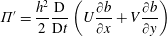 $$\begin{eqnarray}\displaystyle & \displaystyle \unicode[STIX]{x1D6F1}^{\prime }=\frac{h^{2}}{2}\frac{\text{D}}{\text{D}t}\left(U\frac{\unicode[STIX]{x2202}b}{\unicode[STIX]{x2202}x}+V\frac{\unicode[STIX]{x2202}b}{\unicode[STIX]{x2202}y}\right) & \displaystyle\end{eqnarray}$$
 $$\begin{eqnarray}\displaystyle & \displaystyle f_{x}^{\prime }=\frac{h\ddot{h}}{2}\frac{\unicode[STIX]{x2202}b}{\unicode[STIX]{x2202}x}+h\frac{\unicode[STIX]{x2202}b}{\unicode[STIX]{x2202}x}\frac{\text{D}}{\text{D}t}\left(U\frac{\unicode[STIX]{x2202}b}{\unicode[STIX]{x2202}x}+V\frac{\unicode[STIX]{x2202}b}{\unicode[STIX]{x2202}y}\right) & \displaystyle\end{eqnarray}$$
 $$\begin{eqnarray}\displaystyle & \displaystyle f_{y}^{\prime }=\frac{h\ddot{h}}{2}\frac{\unicode[STIX]{x2202}b}{\unicode[STIX]{x2202}y}+h\frac{\unicode[STIX]{x2202}b}{\unicode[STIX]{x2202}y}\frac{\text{D}}{\text{D}t}\left(U\frac{\unicode[STIX]{x2202}b}{\unicode[STIX]{x2202}x}+V\frac{\unicode[STIX]{x2202}b}{\unicode[STIX]{x2202}y}\right) & \displaystyle\end{eqnarray}$$
and
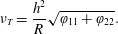 $$\begin{eqnarray}\unicode[STIX]{x1D708}_{T}=\frac{h^{2}}{R}\sqrt{\unicode[STIX]{x1D711}_{11}+\unicode[STIX]{x1D711}_{22}}.\end{eqnarray}$$
Appendix C. Numerical scheme
We consider a computational domain
 $\unicode[STIX]{x1D6FA}\subset \mathbb{R}^{2}$
, discretized with a conformal triangular mesh
 ${\mathcal{T}}_{h}$
. Denoting by
 $T$
a generic element of the triangulation and by
 $\unicode[STIX]{x2202}T$
its boundary, we introduce the broken polynomial space
 $$\begin{eqnarray}\mathbb{P}^{k}({\mathcal{T}}_{h}):=\{v\in L^{2}\mid v_{\mid T}\in \mathbb{P}^{k}(T),\forall T\in {\mathcal{T}}_{h}\},\end{eqnarray}$$
where
 $\mathbb{P}^{k}(T)$
denotes the space of two-variable polynomials in
 $T$
of degree at most
 $k$
. The area of
 $T$
is denoted
 $|T|$
and the notations
 $\mathfrak{h}_{T}$
,
 $\mathfrak{p}_{T}$
will respectively stand for its diameter and perimeter. In the following, the notation
 $N_{k}$
is employed for the number of degrees of freedom, equal to
 $\text{dim}(\mathbb{P}^{k}(T))=(k+1)(k+2)/2$
. The approximation space is
 $X_{h}=\mathbb{P}^{k}(T)\times (\mathbb{P}^{k}(T))^{2}\times (\mathbb{P}^{k}(T))^{3}$
. The computational time interval is denoted
 $[0,t_{max}]$
and discretized in a sequence of intermediate times
 $(t^{n})_{n=0,N}$
with a local time step
 $\unicode[STIX]{x0394}t^{n}=t^{n+1}-t^{n}$
. With notations similar to the continuous frame, we hence seek for an approximate solution
 $\boldsymbol{W}_{h}=(Z_{h},h\boldsymbol{U}_{h}^{\text{T}},h\unicode[STIX]{x1D753}_{11h},h\unicode[STIX]{x1D753}_{12h},h\unicode[STIX]{x1D753}_{22h})$
of (4.18). The resulting semi-discrete formulation can be expressed through the local statement: find
 $\boldsymbol{W}_{h}\in X_{h}$
such that:
 $$\begin{eqnarray}\displaystyle & & \displaystyle \int _{T}\frac{\text{d}}{\text{d}t}\boldsymbol{W}_{h}\unicode[STIX]{x03C0}_{h}\,\text{d}\boldsymbol{x}-\int _{T}\mathbb{F}(\boldsymbol{W}_{h},b_{h})\boldsymbol{\cdot }\mathbf{g}\mathbf{r}\mathbf{a}\mathbf{d}\,\unicode[STIX]{x03C0}_{h}\,\text{d}\boldsymbol{x}+\int _{\unicode[STIX]{x2202}T}\mathbb{F}(\boldsymbol{W}_{h},b_{h})\boldsymbol{\cdot }\boldsymbol{n}_{\unicode[STIX]{x2202}T}\,\unicode[STIX]{x03C0}_{h}\,\text{d}s\nonumber\\ \displaystyle & & \displaystyle \quad +\,\int _{T}\mathbb{D}(\boldsymbol{W}_{h},b_{h})\unicode[STIX]{x03C0}_{h}\,\text{d}\boldsymbol{x}=\int _{T}\mathbb{S}(\boldsymbol{W}_{h},b_{h})\unicode[STIX]{x03C0}_{h}\,\text{d}\boldsymbol{x},\end{eqnarray}$$
for all
 $\unicode[STIX]{x03C0}_{h}\in \mathbb{P}^{k}({\mathcal{T}}_{h})$
and all
 $T\in {\mathcal{T}}_{h}$
. In the formulation above,
 $b_{h}$
stands for a polynomial expansion of the topography
 $b$
on
 $\mathbb{P}^{k}({\mathcal{T}}_{h})$
and
 $\boldsymbol{n}_{\unicode[STIX]{x2202}T}$
is the unit outward normal to the boundary
 $\unicode[STIX]{x2202}T$
. Given a local polynomial expansion basis
 $\{\unicode[STIX]{x1D719}_{i}\}_{i}^{N_{k}}$
, the local restriction of the solution on a given element
 $T$
can be written as:
 $$\begin{eqnarray}\boldsymbol{W}_{h|T}(\boldsymbol{x},t)=\mathop{\sum }_{i=1}^{N_{k}}\boldsymbol{W}_{i}(t)\unicode[STIX]{x1D719}_{i}(\boldsymbol{x}),\quad \boldsymbol{x}\in T,t\in [0,t_{max}],\end{eqnarray}$$
where
 $\{\boldsymbol{W}_{i}\}_{i}^{N_{k}}$
are the local expansion coefficients, so that the formulation (C 2) leads to
 $$\begin{eqnarray}\displaystyle & & \displaystyle \mathop{\sum }_{i=1}^{N_{k}}\frac{\text{d}}{\text{d}t}\boldsymbol{W}_{i}(t)\left(\int _{T}\unicode[STIX]{x1D719}_{i}\unicode[STIX]{x1D719}_{j}\,\text{d}\boldsymbol{x}\right)-\int _{T}\mathbb{F}(\boldsymbol{W}_{h},b_{h})\boldsymbol{\cdot }\mathbf{g}\mathbf{r}\mathbf{a}\mathbf{d}\,\unicode[STIX]{x1D719}_{j}\,\text{d}\boldsymbol{x}+\mathop{\sum }_{F\subset \unicode[STIX]{x2202}T}\int _{F}\widehat{\mathbb{F}}_{T,F}\unicode[STIX]{x1D719}_{j}\,\text{d}s\nonumber\\ \displaystyle & & \displaystyle \quad +\,\int _{T}\mathbb{D}(\boldsymbol{W}_{h},b_{h})\unicode[STIX]{x1D719}_{j}\,\text{d}\boldsymbol{x}=\int _{T}\mathbb{S}(\boldsymbol{W}_{h},b_{h})\unicode[STIX]{x1D719}_{j}\,\text{d}\boldsymbol{x},\quad 1\leqslant j\leqslant N_{k}.\end{eqnarray}$$
In the above expression,
 $\hat{\mathbb{F}}_{T,F}$
are interface terms approximating the projection of the fluxes
 $\mathbb{F}(\boldsymbol{W}_{h},b_{h})\boldsymbol{\cdot }\boldsymbol{n}_{T,F}$
along the unit outward normal corresponding to the face
 $F$
of
 $T$
, defined in the spirit of finite volume methods. In Duran & Marche (Reference Duran and Marche2017), the preservation of motionless steady states
 $Z=\text{cte}$
,
 $\boldsymbol{U}=0$
is guaranteed for solutions of an arbitrary order based on an adaptation of the hydrostatic reconstruction (Audusse et al.
Reference Audusse, Bouchut, Bristeau, Klein and Perthame2004). As a matter of fact, it can be shown easily that the pre-balanced formalism allows a trivial treatment of such configurations, as soon as the line and surface integrals are computed exactly and the topography admits a continuous discrete representation (which is automatically ensured with nodal expansions). As a consequence, with the same choice of nodal expansion basis
 $\{\unicode[STIX]{x1D719}_{i}\}_{i}^{N_{k}}$
for the bathymetry, there is no need to introduce modified states or additional correction term in the numerical fluxes. In light of this, classical Rusanov fluxes are used to evaluate the interface terms:
 $$\begin{eqnarray}\displaystyle \widehat{\mathbb{F}}_{T,F} & = & \displaystyle \mathbb{F}_{h}(\boldsymbol{W}^{-},\boldsymbol{W}^{+},b^{-},b^{+},\boldsymbol{n}_{T,F})\nonumber\\ \displaystyle & = & \displaystyle {\textstyle \frac{1}{2}}(\mathbb{F}(\boldsymbol{W}^{-},b^{-})\boldsymbol{\cdot }\boldsymbol{n}_{T,F}+\mathbb{F}(\boldsymbol{W}^{+},b^{+})\boldsymbol{\cdot }\boldsymbol{n}_{T,F})-a(\boldsymbol{W}^{+}-\boldsymbol{W}^{-}),\end{eqnarray}$$
where the superscripts ‘
 $-/+$
’ refer to the interior and exterior states respectively and
 $a=\max _{T\in {\mathcal{T}}_{h}}\unicode[STIX]{x1D706}_{T}$
,
 $\unicode[STIX]{x1D706}_{T}$
referring to the maximum wave speed at the level of the element
 $T$
:
 $$\begin{eqnarray}\unicode[STIX]{x1D706}_{T}=\max _{\unicode[STIX]{x2202}T}(\boldsymbol{U}\boldsymbol{\cdot }\boldsymbol{n}_{\unicode[STIX]{x2202}T}\pm \sqrt{gh+3h^{2}\boldsymbol{ n}_{\unicode[STIX]{x2202}T}\boldsymbol{\cdot }\unicode[STIX]{x1D753}\boldsymbol{\cdot }\boldsymbol{ n}_{\unicode[STIX]{x2202}T}}).\end{eqnarray}$$
Based on the works of Cockburn & Shu (Reference Cockburn and Shu2001), the associated Courant–Friedrichs–Levy condition is
 $$\begin{eqnarray}\unicode[STIX]{x1D706}_{T}\frac{\mathfrak{p}_{T}}{|T|}\unicode[STIX]{x0394}t^{n}\leqslant \frac{1}{2k+1},\quad \forall T\in {\mathcal{T}}_{h},\end{eqnarray}$$
but the presence of viscous terms in the model may constrain the time step to a parabolic stability condition. This point has to be taken into account during our numerical simulations. An implicit treatment of these terms would allow us to get rid of this restriction, but at the price of partially loose the computational efficiency and the ease of implementation of the method. Such investigations are left for future works.
For the wetting and drying treatment, we used the technique employed in Duran & Marche (Reference Duran and Marche2017), involving the positive-preserving reconstruction introduced in Zhang, Xia, & Shu (Reference Zhang, Xia and Shu2012), coupled with a classical cutoff technique to discriminate wet cells from dry cells. This method was sufficient to stabilize the computations in the vicinity of dry fronts, even in the presence of enstrophy, and without the need for a preliminary thin layer of water.