



1. Introduction
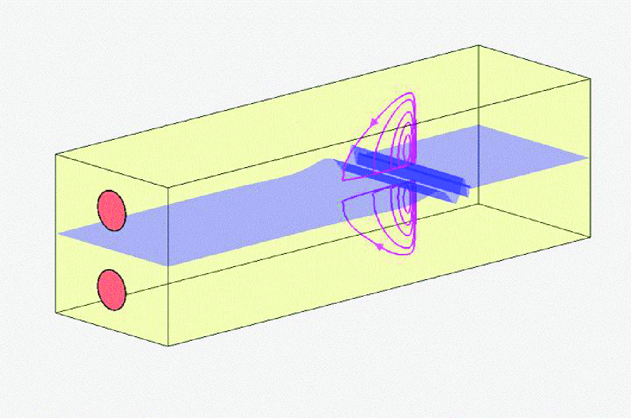
In a laboratory model of the cochlea using a rubber membrane at middle depth, von Békésy (Reference von Békésy1960) found two eddies in the perilymph on opposite sides of the membrane, when periodic pressure is applied at the stapes. Among the observed features, an eddy was found in the immediate neighbourhood of helicotrema at low frequencies, but closer to the stapes at high frequencies. Also, the eddy moves closer to the stapes if the membrane is thicker, or is gradually stiffened during the test due to significant water absorption.
Tonndorf (Reference Tonndorf1970) explained on physical grounds that von Békésy eddies owe their existence to nonlinear convective inertia. This view was recognised by Lesser & Berkley (Reference Lesser and Berkley1972), who also gave a two-dimensional linearised theory of the travelling wave. Extending the classical work of Rayleigh on acoustic streaming in organ pipes, Lighthill (Reference Lighthill1992) began an analytical study of streaming in ears. He also cited evidence that the streaming may cause steady deflection of hair cells, and stimulate neural activity on the reception of a signal. Further numerical details were revealed by the excellent computational studies of Edom (Reference Edom2013) and Edom et al. (Reference Edom, Obrist and Kleiser2014). For comprehensive reviews of the physiology and fluid physics of the inner ear, readers are referred to Dallos, Popper & Fay (Reference Dallos, Popper and Fay1996), Reichenbach & Hudspeth (Reference Reichenbach and Hudspeth2014) and Obrist (Reference Obrist2019).
As is well-known, steady streaming in wavy flows near a stationary wall is caused by Reynolds stresses in the viscous boundary layer, usually much thinner than the wavelength (Rayleigh Reference Rayleigh1884; Schlichting Reference Schlichting1960; Batchelor Reference Batchelor1967). Related phenomena have been found in media of different sizes over a wide range of wave frequencies, such as water waves over a flat sea bed (Longuet-Higgins Reference Longuet-Higgins1953; Hunt & Johns Reference Hunt and Johns1963; Carter, Liu & Mei Reference Carter, Liu and Mei1973) or over a rippled seabed (Hara & Mei Reference Hara and Mei1990), in sound waves in vessels (Lighthill Reference Lighthill1978), and ultra-high-frequency waves in microfluidics (Bruus Reference Bruus2008; Vanneste & Bühler Reference Vanneste and Bühler2011). Additional physics of induced streaming was discovered by Riley (Reference Riley1965) and Stuart (Reference Stuart1966), who found a secondary boundary layer outside the Stokes layer when oscillations are so strong that the stream Reynolds number is not small, i.e.,
 \begin{equation} R_s=\frac {\omega ^2 A^2}{\omega \nu }=O\left ( \frac { A^2}{\delta ^2}\right)=O(1), \end{equation}
where
 $\nu$
is the fluid viscosity,
 $\omega$
is the sound frequency,
 $ A$
is the flow amplitude of oscillations, and
 $\delta ={\sqrt {\nu /\omega }}$
is the thickness of the oscillatory boundary layer. In the human ear, this double layer phenomenon cannot occur, however, as seen by the following estimate. The viscosity of the fluid (perilymph) is
 $\nu =O(1)\,\mbox{mm}^2\,\mbox{s}^{-1}$
. For sound of frequency
 $\omega /2\unicode{x03C0} =2000\,\rm Hz$
to 100 Hz, the resonant displacement of the basilar membrane (BM) near the characteristic place varies from
 $A=0.1\ \unicode{x03BC}\text{m}$
to
 $A=1.0\ \unicode{x03BC} \mbox{m}$
. For example, at
 $f=\omega /2\unicode{x03C0} =1000\,\mbox{Hz}$
, the Stokes layer thickness is
 ${\delta = \sqrt {\nu /\omega }} = 12.6\, \unicode{x03BC} \mbox{m} = O(10\,\unicode{x03BC}\mbox{m})$
. The maximum is
 $A/\delta = 10^{-2}{-}10^{-1}$
, making
 $A\ll \delta \ll h$
. Hence
 $R_s$
is too small for double layers to exist.
To complement existing numerical solutions of two-dimensional Navier–Stokes equations, our first aim here is to provide an analytical examination of the steady streaming in the cochlea. Focus is on weak nonlinearity due to small BM displacement, i.e.
 $A=O(\epsilon \delta)=O(\epsilon ^2h)$
, where
 $\epsilon \ll 1$
. After examining the linearised wave motion by Wentzel-Kramers-Brillouin (WKB) approximation, higher-order details of streaming in the essentially inviscid core and the Stokes boundary layers are worked out. The results will then be used to compare the role of streaming versus the role of molecular diffusion in the transport of a passive scalar, which may be of relevance to drug delivery in the inner ear.
2. Governing equations for a two-dimensional cochlear duct
A two-dimensional model of the cochlea. The BM displacement is exaggerated.

Distinguished by hats, physical variables are normalised by the following scales: half-depth
 $ h$
, oscillation amplitude
 $ A$
, and sound frequency
 $\omega$
. The normalised (hatless) variables are defined by
 \begin{eqnarray} \widehat t = t/\omega,\quad (\widehat x, \widehat z\,)=( x, z)\,h,\quad (\widehat u, \widehat w) = A \omega (u,w), \quad \widehat p=(\rho A\omega ^2 h) p,\quad \widehat b=A b. \end{eqnarray}
Unlike oscillatory flows in blood vessels (Wang & Tarbell Reference Wang and Tarbell1992), where the wavelength is much longer than the vessel radius, sound wavelength in human ears can be so short as to be comparable to the depth of cochlear duct. In dimensionless terms, the cochlea of total depth
 $2 h$
is separated in the middle by the moving BM at
 $z=\epsilon ^2\, b(x,t)$
, where
 \begin{equation} \epsilon ^2 = \frac {A}{h} \ll 1 \end{equation}
is a small parameter that also characterises weak convective inertia. In both the upper duct (scala vestibuli,
 $\epsilon ^2 b \leqslant z \leqslant 1$
) and the lower duct (scala tympani,
 $-1 \leqslant z \leqslant \epsilon ^2 b$
), the flow is governed by the dimensionless Navier–Stokes equations:
 \begin{align} \frac {\partial u}{\partial x}+\frac {\partial w}{\partial z} = 0, \\[-30pt] \nonumber \end{align}
 \begin{align} \frac {\partial u}{\partial t}+ \epsilon ^2\left (\, u\frac {\partial u}{\partial x} +\, w\frac {\partial u}{\partial z} \right) = -\frac {\partial p}{\partial x}+\beta ^2 \epsilon ^2\, \nabla ^2 u,\\[-30pt] \nonumber \end{align}
 \begin{align} \frac {\partial w}{\partial t}+ \epsilon ^2 \left ( u\frac {\partial w}{\partial x}+ w\frac {\partial w}{\partial z} \right) = -\frac {\partial p}{\partial z}+ \beta ^2\epsilon ^2\,\nabla ^2 w, \\[-30pt] \nonumber \end{align}
with
 \begin{equation} \beta ^2 = \frac {1}{\epsilon ^2}\frac {\delta ^2}{h^2} = \frac {h}{A}\frac {\delta ^2}{ h^2} = O(1), \end{equation}
where
 $\beta \epsilon$
signifies the small effect of viscosity. In Lighthill (Reference Lighthill1992), no top wall is considered and the Stokes boundary layer thickness is comparable to the wavelength, which is different from the case considered in this study.
Referring to figure 1, the kinematic boundary conditions are
 \begin{equation} u=0, \quad w = \frac {\partial b}{\partial t}\quad \mbox{at}\ z = \epsilon ^2 b \end{equation}
on the BM, and
 \begin{equation} u=0, \quad w = 0\quad \mbox{at}\ z = 1\ (\mbox{or } z=-1) \end{equation}
on the top (or bottom) wall of the upper (or lower) duct.
As in Lesser & Berkley (Reference Lesser and Berkley1972), we will assume that the oval and round windows at the stapes (
 $x,X=0$
) oscillate in opposite directions:
 \begin{equation} u(x=0,z,t) = \begin{cases} -\,{\mathcal U}_{o} \textrm{e}^{-{\mathrm{i}} t} + {\mbox{c.c.}}, & \epsilon ^2 b \leqslant z \leqslant 1,\\ +\,{\mathcal U}_{o} \textrm{e}^{-{\mathrm{i}} t} + {\mbox{c.c.}}, & -1 \leqslant z \leqslant \epsilon ^2 b, \end{cases} \end{equation}
where
 $\mathcal{U}_o$
is the half-amplitude of the velocities of the oval and round windows, uniform across width
 $-1\leqslant z\leqslant 1$
. The signs on the right-hand side are chosen so that the BM displacement amplitude
 $B_{01}$
defined later (in (3.15)) is positive at
 $x=0$
.
In dimensional form, the linear dynamic boundary condition on the BM is
 \begin{align} m \frac {\partial ^2 \widehat b}{\phantom{\frac{1}{2}}\partial {\widehat{t}}^{\,\,2}} + R \frac {\partial \widehat b}{\partial \widehat t} + K\widehat b = - \widehat p_+ + \widehat p_- \quad \mbox{at}\ \widehat z=\widehat b, \end{align}
where
 $ m, R, K$
are the mass, damping and stiffness per unit area of the BM. All of these vary with
 $\widehat x$
along the duct at the scale of
 $O(5{-}10\ \text{mm})$
, as shown in table 1. In addition,
 $\widehat p_+$
and
 $ \widehat p_-$
are the fluid pressures on the upper and lower sides of the BM, respectively. In more recent studies, (2.10) has been modified by adding a cubic term to examine Hopf bifurcations (Equíluz et al. Reference Eguíluz, Ospeck, Choe, Hudspeth and Magnasco2000; Reichenbach & Hudspeth Reference Reichenbach and Hudspeth2014). But the time scale for such bifurcations due to cubic nonlinearity is much longer than that for steady streaming due to quadratic nonlinearity to be considered here. For this reason, only the linear model (2.10) is considered in this work.
Spatial variations of mass, damping and stiffness of the BM proposed in previous studies. The unit of
 $\widehat x^{\,\prime}$
is centimetres,
 $\widehat x^{\,\prime} = 10\,\widehat x$
, 1 dyn is
 $10^{-5}$
N. The first six citations are compiled by Neely (Reference Neely1981).

Making use of (2.1), (2.10) can be rendered dimensionless to
 \begin{equation} M \left ( \frac {\partial ^2 b}{\partial t^2}+ 2\epsilon f_F\sigma \frac {\partial b}{\partial t} + \sigma ^2 b \right) = -p_+ + p_-\quad \mbox{at}\ z = \epsilon ^2 b, \end{equation}
where
 \begin{eqnarray} M = \frac {m}{\rho h},\quad \epsilon f_F =\frac {R}{2\sqrt {Km}},\quad \sigma =\frac {\sqrt {K/m}}{\omega }=\frac {\text{resonance frequency}}{\text{forcing frequency}}, \end{eqnarray}
with
 $\epsilon f_F$
being the coefficient of internal friction. The parameters have been assumed by past authors to have very different dependences on
 $\widehat x$
, as listed in table 1. Most authors have chosen similar models for
 $m$
and
 $K$
so that the resonance frequency
 $({1}/{2\unicode{x03C0} })\sqrt {{K}/{m}}$
decreases exponentially along the cochlea as shown in figure 2. However, vastly diverse values of the internal friction
 $R(\widehat x\,)$
have been chosen by past authors, as shown in figure 3. Among them Peterson & Bogert (Reference Peterson and Bogert1950) and de Boer & MacKay (Reference de Boer and MacKay1980) have assumed this damping to be negligible. Allen (Reference Allen1977) assumed weak damping,
 $\epsilon f_F = 0.0212$
. On the other hand, Lesser & Berkley (Reference Lesser and Berkley1972) assumed significantly stronger damping,
 $\epsilon f_F = 0.212$
. These diverse assumptions are likely due to the difficulty of measuring local values. Alternatively, Edom et al. (Reference Edom, Obrist and Kleiser2014) represent the BM by an internal force in the momentum equation, and assume
 $m$
and
 $R$
to be zero, but allow both transversal
 $\widehat \eta _y$
and axial
 $\widehat \eta _x$
deflections, with different stiffnesses
 $K_y=K$
and
 $K_x$
. Opinions on the axial deflection appear uncertain (Edom Reference Edom2013), and the value
 $K_x = K_y/100$
was assumed by Edom et al. (Reference Edom, Obrist and Kleiser2014). In the present study, only the transversal displacement of the BM is considered. In this study, we choose weak damping in (2.10) as in Allen (Reference Allen1977). This assumption simplifies the mathematics and yields numerical results consistent with past studies.
Resonant frequencies of the BM models used by past authors.

Internal friction ratio
 ${R}/({2\sqrt {m K}})$
of the BM models used by past authors.

Inside the BM boundary layers of thickness
 $\Delta z=O(\epsilon)$
, we will express all unknowns as the sum of an essentially inviscid part (unprimed) and a viscous part (primed). The primed terms depend on
 $x$
and the BM boundary layer coordinate
 $\zeta = z/\beta \epsilon$
defined later (in (4.4)). It follows from (2.5) that the boundary layer correction for pressure
 $p^{\prime}$
is nearly uniform across the boundary layer:
 \begin{equation} \frac {\partial p^{\prime}}{\partial \zeta } = O(\epsilon ^2),\,\,\mbox{where}\ \zeta = \frac {z}{\beta \epsilon }. \end{equation}
Therefore, up to
 $O(\epsilon)$
, the pressure inside the BM boundary layer is dominated by the inviscid and linear core pressure
 $p = p_0+\epsilon p_1$
at
 $z=0$
, with an error of
 $O(\epsilon ^2)$
. Lesser & Berkley (Reference Lesser and Berkley1972) have shown that
 $ u^-(-z) = -u^+(z)$
,
 $ w^-(-z) = w^+(z)$
and
 $ p^-(-z)=- p^+(z)$
, where the superscripts
 $+$
and
 $-$
represent the upper and lower ducts, respectively, so that
 \begin{equation} \left.p^-\right |_{z=0} = \left. -p^+\right |_{z=0}. \end{equation}
As a consequence, the net pressure acting on the BM is
 \begin{equation} [ -p^+ + p^-]_{z=\epsilon ^2 b} = -2 \big[ p_0^+ + \epsilon \, p_1^+ \big]_{z=0} + O(\epsilon ^2), \end{equation}
where
 $p_0^+, p_1^+$
are the first two terms in the power series of
 $p^+$
. Substituting (2.15) into (2.11), we get
 \begin{eqnarray} O(1):\quad M \left (\frac {\partial ^2}{\partial t^2} + \sigma ^2 \right) b = \left.-2 p^+_0\right |_{z=0}, \end{eqnarray}
 \begin{eqnarray} O(\epsilon):\quad 2 f_F M \sigma \frac {\partial b}{\partial t} = \left. -2 p^+_1\right |_{z=0}. \end{eqnarray}
The kinematic boundary conditions (2.7) and (2.8) apply for the upper duct. In conclusion, the two-duct problem is reduced to that for the upper duct only as in Lesser & Berkley (Reference Lesser and Berkley1972). Hereafter, we will simply use
 $p$
as the pressure in the upper duct for brevity.
3. Approximations in the potential core
In the core, let us define the stream function
 $\psi$
such that
 \begin{equation} u = \frac {\partial \psi }{\partial z},\quad w = -\frac {\partial \psi }{\partial x}. \end{equation}
The dimensionless Navier–Stokes equations (2.4) and (2.5) can be rewritten as
 \begin{eqnarray} \frac {\partial }{\partial t} \frac {\partial \psi }{\partial z} + \epsilon ^2 \left (u\frac {\partial u}{\partial x} + w\frac {\partial u}{\partial z} \right) = -\frac {\partial p}{\partial x} + \beta ^2\epsilon ^2\, \nabla ^2 \frac {\partial \psi }{\partial z}, \end{eqnarray}
 \begin{eqnarray} -\frac {\partial }{\partial t} \frac {\partial \psi }{\partial x} + \epsilon ^2 \left ( u \frac {\partial w}{\partial x} + w\frac {\partial w}{\partial z}\right) = -\frac {\partial p}{\partial z} - \beta ^2\epsilon ^2\, \nabla ^2 \frac {\partial \psi }{\partial x}, \end{eqnarray}
which have been reduced by Rayleigh (Reference Rayleigh1884) to
 \begin{equation} \epsilon ^2 \beta ^2\, \nabla ^4 \psi - \frac {\partial }{\partial t}\nabla ^2 \psi = \epsilon ^2 \left ( u \frac {\partial }{\partial x} + w \frac {\partial }{\partial z} \right) \nabla ^2 \psi, \end{equation}
where
 $\nabla ^2\psi$
is the vorticity
 \begin{equation} \nabla ^2 \psi =\frac {\partial u}{\partial z}-\frac {\partial w}{\partial x}. \end{equation}
If
 $\psi$
and
 $p$
are expanded in power series of
 $\epsilon$
, then
 \begin{eqnarray} && \epsilon ^2\beta ^2\,\nabla ^4\big(\psi _0+\epsilon \psi _1+\epsilon ^2\psi _2+\cdots\big) -\frac {\partial }{\partial t}\nabla ^2\big(\psi _0+\epsilon \psi _1+\epsilon ^2\psi _2+\cdots\big) \nonumber \\ &&\quad =\epsilon ^2\left [ u_0\frac {\partial }{\partial x}+w_0\frac {\partial }{\partial z}\right]\nabla ^2\big(\psi _0+\epsilon \psi _1+\epsilon ^2\psi _2+\cdots\big). \end{eqnarray}
At orders
 $O(\epsilon ^0)$
and
 $O(\epsilon)$
, the momentum equations are approximately linear, and the flow is irrotational:
 \begin{equation} \frac {\partial \nabla ^2\psi _0 }{\partial t}=\frac {\partial \nabla ^2\psi _1}{\partial t}=0,\quad \text{ implying} \quad \nabla ^2\psi _0=\nabla ^2\psi _1=0, \end{equation}
which imply in turn
 \begin{equation} \nabla ^2 p_0=\nabla ^2 p_1 = 0. \end{equation}
Zweig, Lipes & Pierce (Reference Zweig, Lipes and Pierce1976) first applied the WKB approximation to sound propagation in the cochlea that requires the wavelength to be much shorter than the longitudinal length scale of cochlea non-uniformity. Boundary layer effects were not considered. It has been shown by Steele & Taber (Reference Steele and Taber1979) that this approximation is very close to the more accurate numerical solution of Neely (Reference Neely1981). A similar approach was applied by Lighthill (Reference Lighthill1981) and Reichenbach & Hudspeth (Reference Reichenbach and Hudspeth2014). Based on the sharp length contrast
 $h/\ell _{BM} =O(\epsilon)$
, where
 $\ell _{BM}$
is the characteristic scale of longitudinal variation of BM properties, we introduce the fast (
 $x$
) and slow (
 $X=\epsilon x$
) coordinates so that
 $\kappa =\kappa (X)$
, and invoke multiple scale analysis. Let
 \begin{equation} [\psi, u, w, p]=\big\{ \big[\Psi _{01}, U_{01}, W_{01}, P_{01}\big] +\epsilon \big[\Psi _{11}, U_{11}, W_{11}, P_{11}\big]\big\} \,{\textrm{e}^{{\mathrm{i}}\,\Theta (x,t)}}+ {\mbox{c.c.}}+O(\epsilon ^2), \end{equation}
where
 $\Theta (x, t)$
is the wave phase defined by
 \begin{equation} \Theta = S(x) - t,\quad S(x) = \int ^x \kappa (X^{\prime})\,\mathrm{d} x^{\,\prime},\quad X^{\prime}=\epsilon x^{\,\prime}, \end{equation}
and
 \begin{equation} \kappa (X) = {k}(X)\, h = \frac {\partial S}{\partial x} \end{equation}
is the local wavenumber with
 $ kh=O(1)$
.
Using (3.9), it then follows from (3.2) and (3.3) that
 \begin{eqnarray} (P_{01},P_{11}) = \frac {1}{\kappa } (U_{01},U_{11}),\quad \frac {\partial (P_{01},P_{11})}{\partial z} = {\mathrm{i}}\, (W_{01},W_{11}) \end{eqnarray}
at the orders
 $O(\epsilon ^0)$
and
 $O(\epsilon)$
, respectively.
We also get from (3.8) at these orders:
 \begin{eqnarray} \frac {\partial ^2 P_{01} }{\partial z^2} -\kappa ^2P_{01} = 0, \end{eqnarray}
 \begin{eqnarray} \frac {\partial ^2P_{11}}{\partial z^2} -\kappa ^2P_{11} = -{\mathrm{i}}\frac {\partial \kappa }{\partial X}P_{01}-2{\mathrm{i}} \kappa \frac {\partial P_{01}}{\partial X}. \end{eqnarray}
Since (2.11) is linear, we can take the BM displacement to be
 \begin{equation} b= b_0 + O(\epsilon ^2) = \big\{ B_{01}(X)\, \textrm{e}^{{\mathrm{i}}\Theta (x, t)} + {\mbox{c.c.}} \big\} +O(\epsilon ^2). \end{equation}
The kinematic boundary conditions on the lower and upper walls are
 \begin{eqnarray} w_0 = -\frac {\partial \psi _0}{\partial x} = \frac {\partial b_0}{\partial t},\quad\text{i.e.}\quad \frac {\partial P_{01}}{\partial z}=-B_{01},\quad z = 0, \end{eqnarray}
 \begin{eqnarray} \def\lumina\hspace*{-12pt}w_0 = -\frac {\partial \psi _0}{\partial x} =\ 0,\quad\text{i.e.}\quad\frac {\partial P_{01}}{\partial z}=0,\quad z = 1. \end{eqnarray}
The solution of (3.13) is
 \begin{equation} P_{01}= - B_{01} \frac {\cosh \kappa (1-z)}{\kappa \sinh \kappa }, \end{equation}
and the corresponding stream function is
 \begin{equation} \psi _0(X, x, z, t) = \Psi _{01}\, \textrm{e}^{{\mathrm{i}}\Theta } + {\mbox{c.c.}}, \end{equation}
with
 \begin{equation} \Psi _{01} (X, z) = \frac {B_{01}}{\kappa } \frac {\sinh \kappa (1-z)}{\sinh \kappa }. \end{equation}
The associated velocity components are
 \begin{eqnarray} \def\lumina\hspace*{-12pt} u_0 = U_{01}\,\textrm{e}^{{\mathrm{i}}\Theta }+{\mbox{c.c.}},\quad\text{with}\ U_{01} = \frac {\partial \Psi _{01}}{\partial z} = - B_{01} \frac {\cosh \kappa (1-z)}{\sinh \kappa }, \end{eqnarray}
 \begin{eqnarray} w_0 = W_{01}\,\textrm{e}^{{\mathrm{i}}\Theta }+{\mbox{c.c.}},\quad \text{with}\ W_{01} = -{\mathrm{i}} \kappa \Psi _{01} = -{\mathrm{i}} B_{01} \frac {\sinh \kappa (1-z)}{\sinh \kappa }. \end{eqnarray}
On the oscillating BM, (2.16) and (2.17) at orders
 $O(\epsilon ^0)$
and
 $O(\epsilon)$
become
 \begin{align} M(-1+\sigma ^2) B_{01} = -2 P_{01}|_{z=0},\\[-25pt] \nonumber\end{align}
 \begin{align} -2{\mathrm{i}} f_F M \sigma B_{01} = -2 P_{11}|_{z=0}. \end{align}
Equations (3.16) and (3.23) can be combined to a homogeneous condition for
 $P_{01}$
on the BM:
 \begin{equation} \frac {\partial P_{01}}{\partial z}=\frac {2P_{01}}{M(\sigma ^2-1)},\quad z=0. \end{equation}
Together with (3.16), the boundary value problem for
 $P_{01}$
is homogeneous. The eigenvalue condition
 \begin{equation} \kappa \tanh \kappa = \frac {2}{M} \frac {1}{\sigma ^2-1} \end{equation}
is also the dispersion relation between
 $\kappa (X)$
and
 $\sigma (X)$
. Let us denote the characteristic place by
 $X_*$
, where
 $\sigma (X_*)=1$
. If
 $\sigma \gt 1$
, then
 $\kappa$
is real for
 $X\lt X_*$
, i.e.
 $\omega \lt \sqrt {K/m}$
; waves propagate. Otherwise, if
 $\sigma \lt 1$
, then
 $\kappa$
is imaginary for
 $X\gt X_*$
; waves attenuate exponentially. Equation (3.26) is the zero-friction approximation of the fuller dispersion relation
 \begin{equation} \kappa \tanh \kappa =\frac {2}{M}\frac {1}{\sigma ^2-1 -\epsilon (2 {\mathrm{i}} \sigma f_F)}. \end{equation}
Here,
 $\kappa$
is complex for all
 $X$
in the entire cochlea, which leads to more cumbersome mathematics.
To complete the determination of
 $P_{01}$
(or
 $B_{01}$
), we need to examine the solvability of
 $P_{11}$
by including the effect of boundary layers.
The leading-order core velocities
 $u_0, w_0$
are given in (3.21) and (3.22). Explicit expressions of the first-order solutions
 $P_{11},\psi _1$
and
 $u_1, w_1$
will not be needed for examining the mean streaming at order
 $O(\epsilon ^2)$
.
4. Oscillations in boundary layers at
 $\boldsymbol{O(\epsilon ^0)}$

In the oscillatory boundary layers near
 $z=\epsilon ^2 b$
and
 $z=1$
, the total stream function is
 $\widehat \psi +\widehat \psi ^{\prime}$
, where the prime signifies viscous corrections in the BM or top boundary layers, normalised according to
 \begin{equation} \psi ^{\prime} = \frac {\widehat \psi ^{\prime}}{A\omega \delta }. \end{equation}
In physical dimensions, the total stream function is
 \begin{equation} \widehat \psi +\widehat \psi ^{\prime}= h(A\omega)\, \psi +\delta (A \omega)\, \psi ^{\prime} =h(A\omega) (\psi + \epsilon \beta \psi ^{\prime}), \end{equation}
where
 $\psi ^{\prime}$
varies in depth according to the scale
 $ {\delta /h}=\beta \epsilon =O(\epsilon)$
. Hence
 $u$
and
 $u^{\prime}$
are comparable in order, and
 $w^{\prime}=O(\epsilon)\, w$
is much smaller than
 $w$
. The governing equation for the viscous vorticity
 $\psi ^{\prime}$
is obtained by first replacing
 $\psi$
in (3.4) by
 $\psi +\epsilon \beta \psi ^{\prime}$
, and then subtracting (3.4) from the result:
 \begin{equation} \epsilon ^2 \beta ^2\, \nabla ^4 (\epsilon \beta \psi ^{\prime}) - \frac {\partial }{\partial t}\nabla ^2 (\epsilon \beta \psi ^{\prime}) = \epsilon ^2 \left [ (u+u^{\prime}) \frac {\partial }{\partial x}+ (w+w^{\prime})\frac {\partial }{\partial z} \right]\nabla ^2 (\epsilon \beta \psi ^{\prime}). \end{equation}
Let us begin by examining the boundary layer problems at leading orders.
4.1. The BM boundary layer
First, consider the boundary layer near the BM. Let us define the boundary layer coordinate
 \begin{equation} \zeta = \frac {z}{\beta \epsilon },\,\, \end{equation}
and consider
 $\psi ^{\prime}$
,
 $u^{\prime}$
and
 $w^{\prime}$
as functions of
 $(X,x,\zeta,t)$
. The BM displacement is
 $ \zeta _{{BM}} = \epsilon ^2 b/(\beta \epsilon)= \epsilon b_0/\beta +O(\epsilon ^3)$
. Let us expand
 \begin{equation} \mathcal{Y}^{\prime} =\sum _{n=0}^2 \epsilon ^n\, \mathcal{Y}^{\prime}_n(X, x, \zeta, t) + O(\epsilon ^3), \end{equation}
where
 $ \mathcal Y^{\prime}\equiv ( \psi ^{\prime}, u^{\prime}, w^{\prime})$
. The viscous velocities inside the BM boundary layer are
 \begin{equation} u^{\prime}_n = \frac {\partial \psi ^{\prime}_n}{\partial \zeta },\quad n = 0, 1, 2, \end{equation}
 \begin{equation} {w^{\prime}_0 = 0},\quad w^{\prime}_1 = - \beta \frac {\partial \psi ^{\prime}_0}{\partial x}, \quad w^{\prime}_2 = - \beta \frac {\partial \psi ^{\prime}_1}{\partial x} - \beta \frac {\partial \psi ^{\prime}_0}{\partial X}. \end{equation}
Note in particular that
 $w^{\prime}=O(\epsilon)\,u^{\prime}$
in the boundary layer.
Within the boundary layer, the core flow velocities can be expanded in Taylor series about
 $z=0$
:
 \begin{align} (u,w)(X, x, \epsilon \beta \zeta, t) = (u_0,w_0)|_{z=0} + \epsilon \left [ (u_1,w_1) + \beta \zeta \frac {\partial (u_0,w_0)}{\partial z}\right]_{z=0} +O(\epsilon ^2). \end{align}
Substituting (4.5) and (4.8) into (4.3), we get the perturbation equations for
 $\psi ^{\prime}_n$
at the three leading orders
 $n=0,1,2\,$
:
 \begin{eqnarray} && \frac {\partial ^4 \psi ^{\prime}_0}{\partial \zeta ^4} - \frac {\partial ^3 \psi ^{\prime}_0}{\partial t\, \partial \zeta ^2} = 0, \end{eqnarray}
 \begin{eqnarray} && \frac {\partial ^4 \psi ^{\prime}_1}{\partial \zeta ^4} - \frac {\partial ^3 \psi ^{\prime}_1}{\partial t\, \partial \zeta ^2} = \frac {1}{\beta } w_0|_{z=0} \frac {\partial ^3 \psi ^{\prime}_0}{\partial \zeta ^3}, \end{eqnarray}
 \begin{eqnarray} &&\frac {\partial ^4 \psi ^{\prime}_2}{\partial \zeta ^4} -\beta ^2 \frac {\partial ^3 \psi ^{\prime}_0}{\partial t\, \partial x^2} + 2 \beta ^2 \frac {\partial ^4 \psi ^{\prime}_0}{\partial x^2\,\partial \zeta ^2} - \frac {\partial ^3 \psi ^{\prime}_2}{\partial t\, \partial \zeta ^2} = \left ( u_0|_{z=0}+u^{\prime}_0 \right) \frac {\partial ^3 \psi ^{\prime}_0}{\partial x\,\partial \zeta ^2} \nonumber \\ && {}\left.\qquad\; +\left [ \zeta \frac {\partial w_0}{\partial z}\right |_{z=0} + \frac {1}{\beta }\big(w_1|_{z=0}+w^{\prime}_1\big)\right] \frac {\partial ^3 \psi ^{\prime}_0}{\partial \zeta ^3} + \frac {w_0|_{z=0}}{\beta } \frac {\partial ^3 \psi ^{\prime}_1}{\partial \zeta ^3}, \end{eqnarray}
where
 $w^{\prime}_0=0$
from (4.7a
) has been used.
On the BM surface
 $z=\epsilon ^2 b_0$
, i.e.
 $\zeta =\epsilon b_0/\beta$
, we replace
 $u$
and
 $w$
by
 $u+u^{\prime}$
and
 $w+w^{\prime}$
, respectively, in (2.7), and perform Taylor expansions about
 $z=\zeta =0$
up to
 $O(\epsilon ^2)$
, to get
 \begin{align} &\left ( u_0 + \epsilon u_1 + \,\epsilon ^2 u_2 + \epsilon ^2 b_0 \frac {\partial u_0}{\partial z} \right)_{z=0} \nonumber \\ &\qquad{}+\left ( u^{\prime}_0 + \epsilon u^{\prime}_1 + \frac {\epsilon }{\beta } b_0 \frac {\partial u^{\prime}_0}{\partial \zeta } + \epsilon ^2 u^{\prime}_2 + \frac {\epsilon ^2}{\beta } b_0 \frac {\partial u^{\prime}_1}{\partial \zeta } + \frac {\epsilon ^2}{2\beta ^2} b_0^2 \frac {\partial ^2 u^{\prime}_0}{\partial \zeta ^2} \right)_{\zeta =0} = 0, \end{align}
 \begin{align} &\left ( w_0 + \epsilon w_1 + \epsilon ^2 w_2 + \epsilon ^2 b_0 \frac {\partial w_0}{\partial z} \right)_{z=0} +\left ( \epsilon w^{\prime}_1 + \epsilon ^2 w^{\prime}_2 + \frac {\epsilon ^2}{\beta } b_0 \frac {\partial w^{\prime}_1}{\partial \zeta } \right)_{\zeta =0} = \frac {\partial b_0}{\partial t}. \end{align}
Separating different orders in (4.12), the boundary values of
 $u^{\prime}_n$
,
 $n=0, 1, 2$
, can be related to
 $u_n$
and
 $u^{\prime}_{n-1}, u^{\prime}_{n-2},\ldots$
as follows:
 \begin{eqnarray} \left. u^{\prime}_0\right |_{\zeta =0}\, = \big. -u_0\big|_{z=0}, \end{eqnarray}
 \begin{eqnarray} u^{\prime}_1 \big|_{\zeta =0} = -u_1 \big|_{z=0}- \frac {b_0}{\beta } \left.\frac {\partial u^{\prime}_0}{\partial \zeta }\right |_{\zeta =0}, \end{eqnarray}
 \begin{eqnarray} \left. u^{\prime}_2\right |_{\zeta =0} = -\left ( u_2 + b_0 \frac {\partial u_0}{\partial z}\right)_{z=0} -\left ( \frac {b_0}{\beta }\frac {\partial u^{\prime}_1}{\partial \zeta } + \frac {b_0^2}{2\beta ^2} \frac {\partial ^2 u^{\prime}_0}{\partial \zeta ^2} \right)_{\zeta =0}. \end{eqnarray}
The viscous stream functions
 $\psi ^{\prime}_n,\ n = 0, 1, 2$
, can be solved from (4.9)–(4.11) subject to (4.14)–(4.16) at
 $z=\zeta =0$
and the vanishing condition
 $\psi ^{\prime}\to 0$
at
 $\zeta \to \infty$
. In addition to (3.16) for
 $w_0|_{z=0}$
, the boundary values for
 $w_1, w_2$
are readily obtained from (4.13):
 \begin{align} \left. w_1\right|_{z=0} = \left. -w^{\prime}_1\right |_{\zeta =0},\\[-30pt] \nonumber\end{align}
 \begin{align} w_2|_{z=0} = \left. -w^{\prime}_2\right |_{\zeta =0} - b_0 \left.\frac {\partial w_0}{\partial z} \right |_{z=0} -\frac {b_0}{\beta } \left.\frac {\partial w^{\prime}_1}{\partial \zeta }\right |_{\zeta =0}.\\[-12pt] \nonumber \end{align}
Equation (4.18) is listed here for completeness but will not be needed later.
Let us apply the WKB approximation to derive the lower-order solutions for the BM boundary layer:
 \begin{equation} \psi ^{\prime}_0 = \Psi ^{\prime}_{01}(X, \zeta)\, \textrm{e}^{{\mathrm{i}} \Theta }+{\mbox{c.c.}},\quad \psi ^{\prime}_1 = \Psi ^{\prime}_{10}(X, \zeta) + ( \Psi ^{\prime}_{11}(X, \zeta) \,\textrm{e}^{{\mathrm{i}} \Theta }+{\mbox{c.c.}}), \end{equation}
 \begin{equation} \psi ^{\prime}_2 = \Psi ^{\prime}_{20}(x, \zeta) + \sum _{m=1}^2 \Psi ^{\prime}_{2m}(X, \zeta)\, \textrm{e}^{{\mathrm{i}} m\Theta }+{\mbox{c.c.}}, \end{equation}
where
 $\Psi ^{\prime}_{nm}$
is the amplitude of the
 $m$
th harmonic of
 $\psi ^{\prime}_n$
.
Focusing first on the first harmonic:
 \begin{equation} u_{01}^{\prime}=\frac {\partial \Psi ^{\prime}_{01}}{\partial \zeta }\,\textrm{e}^{{\mathrm{i}}\Theta }+{\mbox{c.c.}}, \quad u_{11}^{\prime}=\frac {\partial \Psi ^{\prime}_{11}}{\partial \zeta }\,\textrm{e}^{{\mathrm{i}}\Theta }+{\mbox{c.c.}}, \end{equation}
 \begin{equation} w^{\prime}_{11} = -\beta\, \frac {\partial \left (\Psi ^{\prime}_{01}\,\textrm{e}^{{\mathrm{i}}\Theta }\right)}{\partial x}+{\mbox{c.c.}} \end{equation}
We substitute (4.19a ) into (4.9), to find
 \begin{equation} \frac {\partial ^4 \Psi ^{\prime}_{01}}{\partial \zeta ^4} + {\mathrm{i}}\, \frac {\partial ^2 \Psi ^{\prime}_{01}}{\partial \zeta ^2}=0,\quad \zeta \gt 0. \end{equation}
The boundary conditions are
 \begin{equation} \left.\frac {\partial \Psi ^{\prime}_{01}}{\partial \zeta }\right|_{\zeta =0} = -U_{01}|_{z=0} = \frac {B_{01}}{\tanh \kappa } \quad \mbox{at}\ \zeta =0, \end{equation}
from (4.14) and (3.21), and
 $\Psi ^{\prime}_{01}$
and
 ${\partial \Psi ^{\prime}_{01}}/{\partial \zeta }$
vanish as
 $\zeta \to \infty$
. The solution is
 \begin{equation} \Psi ^{\prime}_{01}(\zeta) = U_{01}|_{z=0} \int _\zeta ^\infty G(\zeta ^{\prime}) \,\mathrm{d} \zeta ^{\prime} = {-\frac {B_{01}}{\tanh \kappa } \frac {\textrm{e}^{-\sqrt {-{\mathrm{i}}}\,\zeta }}{\sqrt {-{\mathrm{i}}}}}, \end{equation}
where
 \begin{equation} G(\zeta) = \textrm{e}^{-\sqrt {-{\mathrm{i}}}\,\zeta },\qquad \text{with}\,\,\,\, \sqrt {- {\mathrm{i}}} \equiv \frac {1- {\mathrm{i}}}{\sqrt {2}}=\textrm{e}^{-{\mathrm{i}} \unicode{x03C0} /4}. \end{equation}
Thus the axial component of the boundary layer velocity is
 \begin{equation} u_{01}^{\prime}=\frac {\partial \Psi ^{\prime}_{01}}{\partial \zeta }\,\textrm{e}^{{\mathrm{i}}\Theta }+{\mbox{c.c.}} =-U_{01}|_{z=0}\,G(\zeta)\,\textrm{e}^{{\mathrm{i}} \Theta }+{\mbox{c.c.}} ={\frac {B_{01}}{\tanh \kappa }\, \textrm{e}^{-\sqrt {-{\mathrm{i}}}\,\zeta + {\mathrm{i}} \Theta }+{\mbox{c.c.}}} \end{equation}
Substituting (4.25) into (4.22), the leading order
 $O(\epsilon)$
transversal component of the boundary layer velocity is
 \begin{equation} w^{\prime}_1= w^{\prime}_{11} = W^{\prime}_{11}\, \textrm{e}^{{\mathrm{i}} \Theta }+{\mbox{c.c.}}, \end{equation}
where
 \begin{equation} W^{\prime}_{11}(X, \zeta) = - {\mathrm{i}} \kappa \beta \, \Psi ^{\prime}_{01} ={{\mathrm{i}} \kappa \beta \frac {B_{01}}{\tanh \kappa } \frac {\textrm{e}^{-\sqrt {-{\mathrm{i}}}\,\zeta }}{\sqrt {-{\mathrm{i}}}}}. \end{equation}
In particular, the boundary value of
 $W_{11}$
at
 $z=0$
is found from (4.17) and (4.29):
 \begin{equation} W_{11}|_{z=0} = -W^{\prime}_{11}|_{\zeta =0} ={\mathrm{i}} \kappa \beta\, \textrm{e}^{{\mathrm{i}}\unicode{x03C0} /4}\, U_{01}|_{z=0} ={-{\mathrm{i}} \kappa \beta \frac {B_{01}}{\tanh \kappa }\, \textrm{e}^{{\mathrm{i}}\unicode{x03C0} /4}}, \end{equation}
which will be needed to determine
 $B_{01}$
.
4.2. Top wall boundary layer
For the region near the top wall, we introduce the boundary layer coordinate
 \begin{equation} { \eta }= \frac {1-z}{\beta \epsilon }. \end{equation}
The top boundary layer solution is easily found:
 \begin{equation} {\Psi }^{\prime}_{01} = -U_{01}|_{z=1} \int ^\infty _{\eta } G(\eta ^{\prime})\,\mathrm{d} \eta ^{\prime} ={\frac {B_{01}}{\sinh \kappa } \frac {\textrm{e}^{-\sqrt {-{\mathrm{i}}}\,\eta }}{\sqrt {-{\mathrm{i}}}}}. \end{equation}
The longitudinal velocity component in the layer is
 \begin{equation} u^{\prime}_{01} = -\frac {\partial \Psi ^{\prime}_{01}}{\partial \eta }\,\textrm{e}^{{\mathrm{i}}\Theta }+{\mbox{c.c.}} =-U_{01}|_{z=1}\,G(\eta)\,\textrm{e}^{{\mathrm{i}} \Theta }+{\mbox{c.c.}} ={\frac {B_{01}}{\sinh \kappa }\, \textrm{e}^{-\sqrt {-{\mathrm{i}}}\,\eta + {\mathrm{i}} \Theta }+{\mbox{c.c.}}}, \end{equation}
and the transversal component is
 \begin{equation} w^{\prime} = w^{\prime}_{11} = W^{\prime}_{11}\,\textrm{e}^{{\mathrm{i}} \Theta }+{\mbox{c.c.}}, \end{equation}
where
 \begin{equation} W^{\prime}_{11}(X, \eta) = -{\mathrm{i}} \kappa \beta \Psi ^{\prime}_{01} = -{\mathrm{i}} \kappa \beta \frac {B_{01}}{\sinh \kappa } \frac {\textrm{e}^{-\sqrt {-{\mathrm{i}}}\,\eta }}{\sqrt {-{\mathrm{i}}}}. \end{equation}
Similar to (4.17), the boundary value of the core velocity
 $W_{11}$
at
 $z=1$
is found as
 \begin{equation} W_{11}|_{z=1} = -W^{\prime}_{11}|_{\eta =0} = -{\mathrm{i}} \kappa \beta\, \textrm{e}^{{\mathrm{i}}\unicode{x03C0} /4}\, U_{01}|_{z=1} = {\mathrm{i}} \kappa \beta \frac {B_{01}}{\sinh \kappa }\, \textrm{e}^{{\mathrm{i}}\unicode{x03C0} /4}. \end{equation}
Both (4.30) and (4.36) are needed in
 $P_{11}$
to complete
 $P_{01}$
and the wave field of
 $O(\epsilon ^0)$
in the inviscid core, as shown below.
5. The
$\boldsymbol{O(\epsilon ^0)}$
waves in the potential core

To ensure the solvability of the inhomogeneous boundary value problem of
 $P_{11}$
, we apply Green’s formula to
 $P_{01}$
and
 $P_{11}$
:
 \begin{align} \!\!\!\!\!\!\int _0^1 \left [ P_{01} \left ( \frac {\partial ^2}{\partial z^2} - \kappa ^2\right) P_{11} - P_{11} \left ( \frac {\partial ^2}{\partial z^2} - \kappa ^2\right) P_{01} \right] \mathrm{d} z = \left [ P_{01} \frac {\partial P_{11}}{\partial z} - P_{11} \frac {\partial P_{01}}{\partial z} \right]_0^1.\quad\, \end{align}
In view of (3.13) and (3.14), the left-hand side of (5.1) becomes
 \begin{eqnarray} \int _0^1 P_{01} \left ( 2 \kappa \frac {\partial P_{01}}{\partial X} + \frac {\partial \kappa }{\partial X} P_{01}\right) \mathrm{d} z = -{\mathrm{i}} \frac {\mathrm{d}}{\mathrm{d} X} \int _0^1 \kappa P_{01}^2 \,\mathrm{d} z. \end{eqnarray}
Using (3.12), (3.22) and (4.36), we get
 \begin{align} \left [ P_{0} \frac {\partial P_{1}}{\partial z} - P_{1} \frac {\partial P_{0}}{\partial z} \right]_{z=1} &= \left [ \frac {U_{0}}{\kappa } \left ( {\mathrm{i}} W_{1} \right) - P_{1} \left ( {\mathrm{i}} W_{0} \right) \right]_{z=1} \notag\\ &= \left.\beta\, \textrm{e}^{{\mathrm{i}} \unicode{x03C0} /4}\, U_{0}^2\right |_{z=1} = \beta\, \textrm{e}^{{\mathrm{i}} \unicode{x03C0} /4}\, \frac {B_{01}^2}{\sinh ^2 \kappa }.\qquad \end{align}
Similar use of (3.12), (3.22), (3.24) and (4.30) gives
 \begin{eqnarray} \left [ P_{01} \frac {\partial P_{11}}{\partial z} - P_{11} \frac {\partial P_{01}}{\partial z} \right]_{z=0} = \left [ \frac {U_{01}}{\kappa } ({\mathrm{i}} { W_{11}}) \!-\! P_{11} ({\mathrm{i}} W_{01}) \right]_{z=0} \nonumber \\ = - \beta\, \textrm{e}^{{\mathrm{i}} \unicode{x03C0} /4}\, \frac {B_{01}^2}{\tanh ^2 \kappa } - {\mathrm{i}} f_F M \sigma B_{01}^2. \end{eqnarray}
With these results, the solvability condition (5.1) becomes
 \begin{eqnarray} -{\mathrm{i}}\, \frac {\mathrm{d}}{\mathrm{d} X}\int _0^1 k\, P^2_{01}(X, z)\, \mathrm{d} z = {{\mathrm{i}} f_F M \sigma B_{01}^2 + \beta\, \textrm{e}^{{\mathrm{i}} \unicode{x03C0} /4}\, B_{01}^2 \left ( \frac {1}{\tanh ^2 \kappa }+\frac {1}{\sinh ^2 \kappa }\right)}. \end{eqnarray}
In view of (3.18) and the integral
 \begin{equation} \int _0^1 \cosh ^2 \kappa (1-z) \mathrm{d} z = \frac {1}{4\kappa }(2 \kappa + \sinh 2 \kappa), \end{equation}
(5.5) becomes an ordinary differential equation for
 $B^2_{01}$
:
 \begin{eqnarray} \frac {\mathrm{d}}{\mathrm{d} X} \left ( \frac {2\kappa +\sinh 2\kappa }{4\kappa ^2 \sinh ^2 \kappa } B_{01}^2\right) = -M \sigma ( f_F + \sqrt {2} \, \textrm{e}^{-{\mathrm{i}} \unicode{x03C0} /4}\, f_V ) B_{01}^2, \end{eqnarray}
where
 \begin{equation} {f_V = \frac {\beta }{\sqrt {2} M \sigma } \left ( \frac {1}{\tanh ^2 \kappa } + \frac {1}{\sinh ^2 \kappa } \right).} \end{equation}
It is shown in Appendix A that (5.7) can also be reduced to
 \begin{equation} \frac {{\rm d}}{{\rm d} X} \left ( C_g E \right) = -\frac {C_g E}{\ell }, \end{equation}
where
 $E$
is the normalised wave energy per unit length of the cochlear duct,
 \begin{equation} E(X) = 2 M \sigma ^2 |B_{01}|^2, \end{equation}
 $C_g(X)$
is the normalised group velocity,
 \begin{equation} C_g (X) =\frac {2}{M\sigma ^2} \frac {2\kappa +\sinh 2\kappa }{4 \kappa ^2 \sinh ^2 \kappa }, \end{equation}
and
 $\ell (X)$
is the dimensionless decay length defined by
 \begin{equation} \frac {1}{\ell (X)} = \frac {1}{\ell _F(X)} + \frac {1}{\ell _V(X)}. \end{equation}
The lengths
 $\ell _F = 2 f_F/(\sigma C_g)$
and
 $\ell _V = 2 f_V/(\sigma C_g)$
represent respectively the spatial distances of decay due to the BM internal friction and boundary layer dissipation.


With the boundary value of
 $B_{01}$
or
 $E$
given at the oval window (
 $X=0$
), the solution is simply
 \begin{equation} \frac {C_g E}{(C_g E)_0} = \exp \left ( -\int _0^X \frac {\mathrm{d} X^{\prime}}{\ell (X^{\prime})} \right), \end{equation}
where
 $(C_g E)_0$
stands for
 $(C_g E)$
evaluated at
 $X=0$
. This result is a slight extension of Steele & Taber (Reference Steele and Taber1979) and Steele & Miller (Reference Steele and Miller1980), who allowed finite BM friction but ignored boundary layer dissipation. Using (5.10) and (5.11), the spatial variation of
 $|B_{01}|^2$
is
 \begin{equation} |B_{01}(X)|^2 = \frac {\left ( 2 M \sigma ^2 C_g |B_{01}|^2\right)_0}{\left ( 2 M \sigma ^2 C_g \right)_X} \exp \left ( -\int _0^X \frac {\mathrm{d} X^{\prime}}{\ell (X^{\prime})} \right), \end{equation}
where
 $(\cdot)_X$
stands for
 $(\cdot)$
evaluated at
 $X$
. In figure 4, the amplitudes and phases of
 $B_{01}$
are plotted in physical dimensions for three frequencies,
 $f = 500, 1000, 2000$
Hz, assuming the same velocity amplitude
 $30\,\unicode{x03BC}\mbox{m}\ \text{s}^{-1}$
at the oval window. It can be shown after some algebra that the downslope portion of (5.14) can be reduced to
 \begin{equation} |B_{01}(X)| \approx |B_{01}(X_p)|\, \frac { \dfrac {1}{X_*-X} \exp \left ( -\dfrac {\alpha }{X_*-X}\right) }{ \dfrac {1}{X_*-X_p} \exp \left ( -\dfrac {\alpha }{X_*-X_p}\right) },\quad X_p \leqslant X \leqslant X_*, \end{equation}
where
 $\alpha$
is the length scale
 \begin{equation} \alpha = \frac {f_F+f_{V_*}}{M \left ( {\mathrm{d} \sigma }\!/ {\mathrm{d} X}\right)_*^2}. \end{equation}
Here,
 $X_*$
is the characteristic place where
 $\sigma (X_*)=1$
, where
 $(\cdot)_*$
signifies evaluation at
 $X_*$
, and
 $X_p$
is the location of the peak of
 $|B_{01}|$
as marked in figure 4(a) for
 $f=1000\,\mbox{Hz}$
.
In figure 4(a), both (5.14) (solid curves) and the approximation of (5.15) for the downslope of
 $|B_{01}|$
(circles) are plotted. The maximum BM amplitude occurs at
 $\widehat x \approx 21.57, 17.55, 13.51$
mm for these frequencies, from the lowest (500 Hz) to the highest (2000 Hz). Figure 4(b) shows that before reaching the peak, the phase change in
 $B_{01}$
is less than
 $O(0.1\unicode{x03C0})$
. The phase increases rapidly to approximately
 $(5{-}10)\unicode{x03C0}$
after passing the peaks. These findings are consistent with previous analytical results for the complex dispersion relation by Allen (Reference Allen1977, figure 7) and Neely (Reference Neely1981, figure 4).
In this numerical example, the cochlear depth
 $h = 1\,\mbox{mm}$
and the BM parameters by Allen (Reference Allen1977) (see table 1) are taken. From (2.9), the amplitude of the oval window velocity is assumed to be
 $2\,\widehat {\mathcal U}_{o} =2A\omega \, \mathcal{U}_o= 30\,\unicode{x03BC}\mbox{m}\,{\rm s^-{^1}}$
, which corresponds to a sound pressure level 76 dB at
 $f = 1000\,\mbox{Hz}$
(Sim et al. Reference Sim, Chatzimichalis, Lauxmann, Röösli, Eiber and Huber2010; Edom et al. Reference Edom, Obrist and Kleiser2014), and is typical in a noisy restaurant or in busy city traffic. For illustration, we choose
 $A = 2\,\widehat {\mathcal{U}}_o/\omega = {30}/{2\unicode{x03C0} f} \ \unicode{x03BC}\text{m}= 9.55, 4.77, 2.39\ \mbox{nm}$
for
 $f = 500, 1000, 2000$
Hz, respectively. Correspondingly, the nonlinearity parameter is
 $\epsilon =\sqrt {A/h}=(3.09, 2.18, 1.55) \times 10^{-3}$
, respectively.
As shown in figure 2, the resonance frequency at the oval window
 $X=0$
is approximately 20 000 Hz in Allen’s model, which is much higher than
 $f=O(1000\,\mbox{Hz})$
under consideration. Therefore, at the oval window
 $X=0$
,
 $\sigma \gg 1$
so that
 \begin{equation} \kappa \approx \tanh \kappa \approx \sqrt {\frac {2}{M}\frac {1}{\sigma ^2|_{X=0}-1}} \approx \sqrt {\frac {2}{M}} \frac {1}{\sigma |_{X=0}}\ll 1 \quad \mbox{at}\ X = 0, \end{equation}
according to the dispersion relation (3.26). In view of (3.21),
 $U_{01}(X=0,z) \approx -B_{01} (X=0)/\tanh \kappa \approx -B_{01}(X=0)/\kappa$
is approximately constant over the oval window. After using (2.9), we find the boundary values for
 $B_{01}$
:
 \begin{equation} B_{01}(X=0) \approx -\kappa U_{01}(X=0, z) = \kappa \,\mathcal{U}_o = \frac {\kappa }{2}. \end{equation}
Figures 5 and 6 show the dimensional wavelength
 $2\unicode{x03C0} /k$
and group velocity
 $\widehat C_{g}=A \omega C_g$
, respectively, for
 $f = 500, 1000, 2000$
Hz. Figure 7 shows the longitudinal variations of the decay length,
 $h\ell /\epsilon$
,
 $h\ell _F/\epsilon$
and
 $h\ell _V/\epsilon$
. All of these quantities decay along the cochlea from the oval window, and fall to zero rapidly when approaching the characteristic place where
 $\sigma (X_*) = 1$
. As shown in figure 7, the decay is dominated by viscous dissipation near the oval window where
 $\ell \approx \ell _V$
, and by the BM friction instead near the characteristic place where
 $\ell \approx \ell _F$
.
Dimensional BM wavelength
 $2\unicode{x03C0} /\kappa$
.

Dimensional BM group velocity
 $\widehat C_{g}= A \omega C_g = ({\partial \omega }/{\partial k})$
.

Dimensional decay lengths:
 $h \ell /\epsilon$
(thick solid line),
 $h \ell _F/\epsilon$
(thin solid line) and
 $h \ell _V/\epsilon$
(dashed line) for
 $f = 1000\,\mbox{Hz}$
.

The leading-order BM displacement
 $\widehat b = A ( B_{01}\,\textrm{e}^{{\mathrm{i}}\,\Theta (x, t)}+{\mbox{c.c.}})$
at
 $t = 0$
(red solid line),
 $t = \unicode{x03C0}/{2}$
(green dashed line) and
 $t=pi$
(blue solid line) for
 $f = 1000\,\mbox{Hz}$
. The envelope
 $\pm 2 A |B_{01}|$
is represented by black dashes.

Figure 8 shows the BM displacement at three instants
 $t = 0, \unicode{x03C0}/{2}, \unicode{x03C0}$
for
 $f = 1000\,\mbox{Hz}$
. The BM crests advance towards the apex, and the peak amplitude is approximately 80 nm, consistent with the estimate 100 nm (0.1
 $\mu$
m) for BM amplitude in § 1.
At
 $O(\epsilon)$
, the oscillatory flow in the core is not needed for calculating the mean streaming at
 $O(\epsilon ^2)$
and is thus not pursued. We now turn to the
 $O(\epsilon)$
dynamics inside the BM and top boundary layers.
6. Oscillations in boundary layers at
$\boldsymbol{O(\epsilon)}$

6.1. The BM boundary layer
Inside the BM boundary layer, the viscous stream functions
 $\psi ^{\prime}_1, \psi ^{\prime}_2,\ldots$
are forced by quadratic forcing terms. Hence higher harmonics will appear. The
 $m$
th harmonic of
 $\psi ^{\prime}_n$
will be denoted by
 $\Psi ^{\prime}_{nm}$
.
Consider the
 $O(\epsilon)$
part of (4.10). Due to BM oscillations at
 $O(\epsilon ^0)$
, a zeroth harmonic emerges, whose amplitude must satisfy
 \begin{equation} \frac {\partial ^4 \Psi ^{\prime}_{10}}{\partial \zeta ^4} = \frac {1}{\beta }\left ( {\mathrm{i}} B^*_{01} \frac {\partial ^3 \Psi ^{\prime}_{01}}{\partial \zeta ^3}+ {\mbox{c.c.}} \right), \end{equation}
and be subjected to
 \begin{equation} \frac {\partial \Psi ^{\prime}_{10}}{\partial \zeta }=- \frac {1}{\beta }\left ( B^*_{01} \frac {\partial ^2 \Psi ^{\prime}_{01}}{\partial \zeta ^2}+{\mbox{c.c.}} \right)\quad \mbox{at}\ \zeta = 0. \end{equation}
Integrating (6.1) in
 $\zeta$
three times, and requiring (6.2) at
 $\zeta =0$
and
 $\Psi ^{\prime}_{10}\to 0$
as
 $\zeta \to \infty$
, we get the steady streaming at
 $O(\epsilon)$
:
 \begin{equation} u^{\prime}_{10} = \frac {\partial \Psi ^{\prime}_{10}}{\partial \zeta } = \frac {1}{\beta } \left ( {\mathrm{i}} B^*_{01} \Psi ^{\prime}_{01} + {\mbox{c.c.}} \right) = - \frac {1}{\beta }\left ( B^*_{01} \frac {\partial ^2 \Psi ^{\prime}_{01}}{\partial \zeta ^2}+{\mbox{c.c.}}\right). \end{equation}
Integrating (6.3) in
 $\zeta$
once more, and using (4.25), we obtain
 \begin{align} \Psi ^{\prime}_{10} =\int _\infty ^\zeta \frac {\partial \Psi ^{\prime}_{10}}{\partial \zeta ^{\prime}}\, \mathrm{d} \zeta ^{\prime} &= -\frac {1}{\beta } \int _\infty ^\zeta B^*_{01} \frac {\partial ^2 \Psi ^{\prime}_{01}}{\partial \zeta ^2}\, \mathrm{d} \zeta ^{\prime} + {\mbox{c.c.}} = \frac {1}{\beta } \left ( B^*_{01} U_{01}|_{z=0}\, G + {\mbox{c.c.}} \right)\nonumber \\ & = -\frac {2}{\beta } \frac {|B_{01}|^2}{\tanh \kappa }\, {\mbox{Re}}\left ( G\right) =-\frac {2}{\beta } \frac {|B_{01}|^2}{\tanh \kappa }\, \textrm{e}^{-\zeta /\sqrt {2}}\cos \frac {\zeta }{\sqrt {2}}, \end{align}
where
 $G$
is given by (4.26). Using (6.4), (6.3) becomes more explicitly
 \begin{eqnarray} \overline {u^{\prime}_1} = u^{\prime}_{10} = \frac {\partial \Psi ^{\prime}_{10}}{\partial \zeta } = \frac {2}{\beta } \frac {|B_{01}|^2}{\tanh \kappa }\, \textrm{e}^{-\frac {\zeta }{\sqrt {2}}} \cos \left ( \frac {\zeta }{\sqrt {2}}-\frac {\unicode{x03C0} }{4} \right). \end{eqnarray}
This relatively strong streaming of
 $O(\epsilon)$
is caused by the oscillating BM, represented by the right-hand side of (4.10). Following (6.5),
 $\overline {u^{\prime}_1}$
is directed from the base towards the apex when
 $-{\unicode{x03C0} }/{4} \leqslant {\zeta }/{\sqrt {2}}-{\unicode{x03C0} }/{4} \lt {\unicode{x03C0} }/{2}$
, i.e.
 $0 \leqslant \zeta \lt 3\sqrt {2}\unicode{x03C0} /4$
, and then turns back towards the base before essentially vanishing for
 $\zeta \gt 7\sqrt {2}\unicode{x03C0} /4$
. As a side remark, in sound waves over a flat wall, or water waves over a flat sea bed, the induced streaming is much weaker (of order
 $O(\epsilon ^2)$
) because the solid boundary is stationary (Longuet-Higgins Reference Longuet-Higgins1953; Batchelor Reference Batchelor1967).
In view of (4.7b
) and (6.4), the transverse viscous streaming is negligible at
 $O(\epsilon)$
:
 \begin{equation} w^{\prime}_{10}= \overline {w^{\prime}_1} =-\beta \overline {\frac {\partial \psi ^{\prime}_1}{\partial x}}=-\beta \frac {\partial \Psi ^{\prime}_{10}}{\partial x} = 0. \end{equation}
At order
 $O(\epsilon)$
, the oscillatory part
 $\Psi ^{\prime}_{11}$
of the boundary layer flow must satisfy
 \begin{equation} \frac {\partial ^4 \Psi ^{\prime}_{11}}{\partial \zeta ^4} + {\mathrm{i}}\, \frac {\partial ^2 \Psi ^{\prime}_{11}}{\partial \zeta ^2} = 0, \quad \zeta \gt 0, \end{equation}
and the boundary condition on the BM
 \begin{equation} \frac {\partial \Psi ^{\prime}_{11}}{\partial \zeta }=-U_{11}|_{z=0} =- \kappa P_{11}|_{z=0} = -{\mathrm{i}} \kappa f_F M \sigma B_{01} \quad \mbox{at}\ \zeta =0, \end{equation}
in view of (3.12) and (3.24), and vanishes at large
 $\zeta$
. Similar to
 $\Psi ^{\prime}_{01}$
of (4.25), the solution of
 $\Psi ^{\prime}_{11}$
is
 \begin{equation} \Psi ^{\prime}_{11}(\zeta) = U_{11}|_{z=0} \int _\zeta ^\infty G(\zeta ^{\prime}) \,\mathrm{d} \zeta ^{\prime} { = {\mathrm{i}} \kappa f_F M \sigma B_{01} \frac {\textrm{e}^{-\sqrt {-{\mathrm{i}}}\,\zeta }}{\sqrt {-{\mathrm{i}}}}}. \end{equation}
The corresponding axial velocity has amplitude
 \begin{equation} U^{\prime}_{11} = \frac {\partial \Psi ^{\prime}_{11}}{\partial \zeta } = -U_{11}|_{z=0}\, G(\zeta) { = -{\mathrm{i}} \kappa f_F M \sigma B_{01}\, \textrm{e}^{-\sqrt {-{\mathrm{i}}}\,\zeta } }. \end{equation}
The transversal component
 $W^{\prime}_{11}$
has been found earlier, in (4.29).
6.2. Top wall boundary layer
Inside the top wall boundary layer,
 $0\lt \eta \lt \infty$
, the viscous part has no time average:
 \begin{equation} \Psi ^{\prime}_{10} = 0,\quad \overline {u^{\prime}_1} = 0, \quad 0\lt \eta \lt \infty, \end{equation}
where
 $\eta$
is defined in (4.31). The first harmonic solution is similar to (4.32),
 \begin{equation} {\Psi }^{\prime}_{11} = -U_{11}|_{z=1} \int ^\infty _{\eta } G(\eta ^{\prime})\mathrm{d} \eta ^{\prime}, \quad 0\lt \eta \lt \infty, \end{equation}
and the corresponding velocity components are
 \begin{equation} U^{\prime}_{11} = -\frac {\partial \Psi ^{\prime}_{11}}{\partial \eta } = -U_{11}|_{z=1}\, G (\eta), \quad W^{\prime}_{11} = -{\mathrm{i}} \kappa \Psi ^{\prime}_{11},\quad 0\lt \eta \lt \infty. \end{equation}
The explicit expression for
 $U_{11}|_{z=1}$
is not needed to obtain the
 $O(\epsilon ^2)$
streaming, hence it is omitted here.
We now turn to the Eulerian streaming at order
 $O(\epsilon ^2)$
.
7. Eulerian streaming at
$\boldsymbol{O(\epsilon ^2)}$

7.1. Streaming in the potential core
Recall from (3.6) that the
 $O(\epsilon ^2)$
part gives
 \begin{equation} \epsilon ^2\beta ^2\,\nabla ^4\psi _0 -\epsilon ^2\frac {\partial }{\partial t}\nabla ^2\psi _2=\epsilon ^2\left [ u_0\frac {\partial }{\partial x}+w_0\frac {\partial }{\partial z}\right]\nabla ^2\psi _0. \end{equation}
In view of (3.7), we conclude that
 \begin{equation} \frac {\partial }{\partial t}\nabla ^2\psi _2=0,\quad\text{i.e.}\quad \nabla ^2\psi _2=\nabla ^2\overline {\psi _2}. \end{equation}
Taking the period average of (3.6), we get, at
 $O(\epsilon ^4)$
,
 \begin{eqnarray} \epsilon ^4 \beta ^2\, \nabla ^4\overline { \psi _2 } = \epsilon ^4 \beta ^2 \frac {\partial ^4 \Psi _{20}}{\partial z^4} = \epsilon ^4\overline { \left ( u_0 \frac {\partial }{\partial x} + w_0 \frac {\partial }{\partial z} \right) \nabla ^2 \overline {\psi _2}}=0. \end{eqnarray}
Let the solution be of the form
 \begin{equation} \Psi _{20}(X, z) = a_0(X) + a_1(X)\, z + a_2(X)\, z^2 + a_3(X)\, z^3. \end{equation}
Four boundary conditions are needed to find
 $a_0,a_1,a_2,a_3$
.
First, there is no normal flux on the top wall:
 \begin{equation} \Psi _{20}|_{z=1} = 0. \end{equation}
Next, the flow cannot pass beyond the characteristic place where
 $\sigma =1$
. Hence the total mean flux at any
 $x$
along the cochlea must vanish:
 \begin{equation} 0=\overline {(\psi + \epsilon \beta \psi ^{\prime})}_{z=1, \eta =0} - \overline {(\psi + \epsilon \beta \psi ^{\prime})}_{z=\epsilon ^2 b},\quad 0 \lt x \lt L. \end{equation}
Using (3.9) and (4.5), and expanding
 $\psi _n$
at
 $z=\epsilon ^2 b_0$
and
 $\psi ^{\prime}_n$
at
 $\zeta ={\epsilon b_0}/{\beta }$
, we get the first average above, i.e.
 \begin{eqnarray} \overline {(\psi + \epsilon \beta \psi ^{\prime})}_{z=1, \eta =0} = \epsilon ^2\, \overline {\psi _2}|_{z=1} = \epsilon ^2 \Psi _{20}|_{z=1}, \end{eqnarray}
and the second average
 \begin{eqnarray} \overline {(\psi + \epsilon \beta \psi ^{\prime})}_{z=\epsilon ^2 b} = \epsilon ^2 \overline { \left ( \psi _2 + b_0 \frac {\partial \psi _0}{\partial z}\right)}_{z=0} + \epsilon \beta \overline { \left ( \epsilon \psi ^{\prime}_1 + \epsilon \frac {b_0}{\beta } \frac {\partial \psi ^{\prime}_0}{\partial \zeta }\right)}_{\zeta =0}, \end{eqnarray}
where errors of
 $O(\epsilon ^3)$
are omitted. Substituting these results into (7.6), and using (7.5) and (6.4), the second boundary condition for
 $\Psi _{20}$
at
 $z=0$
is found:
 \begin{equation} \Psi _{20}|_{z=0} = \overline {\psi _2}|_{z=0} = -\overline { \left ( b_0 \frac {\partial \psi _0}{\partial z}\right)}_{z=0} = -B^*_{01} U_{01}|_{z=0}+{\mbox{c.c.}} = \frac {2}{\tanh \kappa } |B_{01}|^2. \end{equation}
Two more boundary conditions for
 ${\partial \Psi _{20}}/{\partial z}$
are still needed.
Consider first the BM. Taking the time average of (4.16), we get
 \begin{equation} \left.\frac {\partial \Psi _{20}}{\partial z}\right |_{z=0} =\overline {u_2}|_{z=0} = -\overline {u^{\prime}_2}|_{\zeta =0} - \left.\overline {b_0 \frac {\partial u_0}{\partial z}}\right |_{z=0} \left. - \frac {1}{\beta }\,\overline {b_0 \frac {\partial u^{\prime}_1}{\partial \zeta }}\right |_{\zeta =0}. \end{equation}
From (7.23) that will be obtained later,
 \begin{equation} \left.\overline {u^{\prime}_2}\right |_{\zeta =0} = -3k\,|U_{01}|^2_{z=0} + \frac {1}{\beta } \left ( B_{01}^* U_{11}|_{z=0}\, \frac {\mathrm{d} G}{\mathrm{d} \zeta } + {\mbox{c.c.}} \right). \end{equation}
Using (4.6) and (6.9), the last term of (7.10) is
 \begin{equation} \frac {1}{\beta }\, \left.\overline {b_0 \frac {\partial u^{\prime}_1}{\partial \zeta }}\right |_{\zeta =0} = \frac {1}{\beta } \left ( B_{01}^* \frac {\partial ^2 \Psi ^{\prime}_{11}}{\partial \zeta ^2}+{\mbox{c.c.}}\right) = -\frac {1}{\beta } \left ( B_{01}^* U_{11}|_{z=0}\, \frac {\mathrm{d} G}{\mathrm{d} \zeta }+{\mbox{c.c.}}\right), \end{equation}
which cancels out the second term of (7.11). In view of (3.7) and (3.16), the second term of
 $\overline {u_2}|_{z=0}$
in (7.10) becomes
 \begin{eqnarray} \Biggl.\overline {b_0 \frac {\partial u_0}{\partial z}}\Biggr|_{z=0} =\left.\overline {\frac {\partial w_0}{\partial x}\int ^t w_0\, \mathrm{d} t^{\prime}}\right |_{z=0} =-\kappa\, \left.\overline {\frac {\partial w_0}{\partial t}\int ^t w_0\, \mathrm{d} t^{\prime}}\right |_{z=0} = 2 \kappa |W_{01}|^2_{z=0}. \end{eqnarray}
With these results, we find from (7.10) the third boundary condition at
 $z=0$
:
 \begin{equation} \left.\frac {\partial \Psi _{20}}{\partial z}\right |_{z=0}=\overline {u_2}|_{z=0} =3 \kappa \, |U_{01}|^2_{z=0} - 2 \kappa |W_{01}|^2_{z=0} = \left ( \frac {3\kappa }{\tanh ^2 \kappa } - 2 \kappa \right) |B_{01}|^2, \end{equation}
which is directed towards the apex.
Since
 $\overline {u_2}|_{z=1} +\overline {u^{\prime}_2}|_{\eta =0} = 0$
at the top wall, the fourth boundary condition for
 $\Psi _{20}$
is, after using (7.27) that will be obtained later,
 \begin{equation} \left.\frac {\partial \Psi _{20}}{\partial z}\right |_{z=1} = \overline {u_2}|_{z=1} = \left.-\overline {{u}^{\prime}_2}\right |_{\eta =0} = 3 \kappa | U_{01} |^2_{z=1} = \frac {3 \kappa }{\sinh ^2 \kappa } |B_{01}|^2. \end{equation}
Close to the oval window,
 $\kappa$
is small. This boundary velocity is approximately
 $3|B_{01}|^2/\kappa$
, equal to the leading term of (7.14) near the BM. Near the characteristic place where
 $\sigma =1$
,
 $\kappa$
is large and (7.15) tends to vanish rapidly.
The solution of (7.4) satisfying all four boundary conditions (7.5), (7.9), (7.14) and (7.15) is finally found:
 \begin{align} \Psi _{20} &= |B_{01}|^2 \left [ ( 2 z^3-3 z^2+1 ) \frac {2}{\tanh \kappa } + ( z^3-2 z^2+z) \left( \frac {3 k}{\tanh ^2 \kappa } - 2 \kappa \right) \right. \nonumber \\ &{}\qquad \qquad +\left.( z^3 - z^2) \frac {3\kappa }{\sinh ^2 \kappa } \right] \end{align}
and
 \begin{align} \overline {u_2} = \frac {\partial \Psi _{20}}{\partial z} &= |B_{01}|^2 \left [ \frac {12 (z^2-z) }{ \tanh \kappa } +(3 z^2 - 4 z + 1) \left ( \frac {3 k}{\tanh ^2 \kappa } - 2\kappa \right) \right.\nonumber \\ &\qquad\qquad \left. {}+ (3 z^2 - 2 z)\frac {3 \kappa }{\sinh ^2 \kappa }\right]. \end{align}
We define the Eulerian stream function and the longitudinal Eulerian current in the core by
 $\Psi _E$
and
 $U_E$
as follows:
 \begin{equation} \Psi _E = \epsilon ^2\Psi _{20}(X, z), \quad U_E(X,z)= \frac {\partial \Psi _E}{\partial z} = \epsilon ^2\, \overline {u_2}. \end{equation}
The transverse component of the Eulerian current is of higher order:
 \begin{equation} W_E(X,z)=\epsilon ^3\, \overline {w_3}, \end{equation}
with
 \begin{align} \overline {w_3} = -\frac {\partial \Psi _{20}}{\partial X} &= -\big(2z^3-3z^2+1\big)\, \frac {\mathrm{d}}{\mathrm{d} X} \left [\frac {2}{\tanh \kappa } |B_{01}|^2\right]\nonumber \\[4pt] &\quad {}-\big(z^3-2z^2+z\big)\, \frac {\mathrm{d}}{\mathrm{d} X}\left [ \left ( \frac {3 \kappa }{\tanh ^2 \kappa } - 2 \kappa \right) |B_{01}|^2 \right] \nonumber \\[4pt] &\quad {}- \big(3z^2-2z\big)\, \frac {\mathrm{d}}{\mathrm{d} X} \left [ \frac {3\kappa }{\sinh ^2 \kappa } |B_{01}|^2 \right]. \end{align}
Sample boundary values of
 $\overline {u_2}$
at
 $z=0$
(BM) and
 $z=1$
(top) are plotted in figure 9. In comparison,
 $\overline {u_2}$
along the BM is of order
 $O(0.01 {-} 0.1\,{\mu}\,\mbox{m}\,{\rm s^-{^1}})$
, much greater than that along the top wall. Numerical results of
 $\kappa$
corresponding to the maximum
 $\overline {u_2}$
in figure 9 are large: 8.70, 9.56, 10.52 for
 $f=500, 1000, 2000$
Hz, respectively, so that
 $\tanh \kappa \approx 1$
and
 $\kappa /\sinh ^2 \kappa \approx 0$
. Thus the maximum
 $\Psi _{20}$
occurs close to
 $z = {1}/{3}$
, where, from (7.17),
 $\overline {u_2}\approx \kappa |B_{01}|^2\, (3z^2-4z+1)=0$
and the maximum value of
 $\Psi _{20, max }$
is approximately
 $4\kappa |B_{01}|^2/27$
.
Dimensional Eulerian streaming velocity
 ${\widehat U}_E=\epsilon ^2 A \omega \,\overline {u_2}=\epsilon ^2 A \omega\, ({\partial \Psi _{20}}/{\partial z})$
at the top (
 $z=1$
) and the lower (
 $z=0$
) core boundaries.

7.2. Viscous streaming in boundary layers
First, consider the BM boundary layer. The time average of (4.11) gives the governing equation for
 $\overline {\psi ^{\prime}_2}=\Psi ^{\prime}_{20}$
:
 \begin{align} \frac {\partial ^4 \Psi ^{\prime}_{20}}{\partial \zeta ^4} &= \overline {\left ( u_0|_{z=0} + u^{\prime}_0 \right) \frac {\partial ^3 \psi ^{\prime}_0}{\partial x\,\partial \zeta ^2}} + \overline { \left ( w_1|_{z=0}+ \zeta \left.\frac {\partial w_0}{\partial z}\right |_{z=0} + w^{\prime}_1\right) \frac {\partial ^3 \psi ^{\prime}_0}{\partial \zeta ^3}} + \overline { w_0|_{z=0} \frac {\partial ^3 \psi ^{\prime}_1}{\partial \zeta ^3}}, \end{align}
which represents the balance between time-averaged diffusion and transport of vorticity
 ${\partial ^2 \psi ^{\prime}_0}/{\partial \zeta ^2}$
. Similar to the Reynolds stress in turbulence, the first term on the right-hand side represents axial convection, and the second and third terms represent transversal convection
 ${\partial ^2 \psi ^{\prime}_0}/{\partial \zeta ^2}$
and
 ${\partial ^2 \psi ^{\prime}_1}/{\partial \zeta ^2}$
in the Stokes layer. Details for solving (7.21) are given as (B7) and (B9) in Appendix B. The explicit results are
 \begin{align} \Psi ^{\prime}_{20} &= \kappa |U_{01}|^2_{z=0}\int _\infty ^\zeta K(\zeta ^{\prime})\, \mathrm{d} \zeta ^{\prime} + \frac {1}{\beta } \left ( B_{01}^* U_{11}|_{z=0} \,{G}(\zeta) + {\mbox{c.c.}} \right) \nonumber \\ &= { \frac {\kappa |B_{01}|^2}{\tanh ^2 \kappa } \int _\infty ^\zeta K(\zeta ^{\prime})\, \mathrm{d} \zeta ^{\prime}- \frac {2}{\beta } \kappa |B_{01}|^2\, f_F M \sigma \, \textrm{e}^{-{\zeta }/{\sqrt {2}}} \sin \frac {\zeta }{\sqrt {2}},} \end{align}
 \begin{align} u^{\prime}_{20} = \overline {u^{\prime}_2} = \frac {\partial \Psi ^{\prime}_{20}}{\partial \zeta } &= \kappa |U_{01}|^2_{z=0}\, K(\zeta) + \frac {1}{\beta }\left ( B_{01}^* U_{11}|_{z=0}\, \frac {\mathrm{d} G}{\mathrm{d} \zeta } + {\mbox{c.c.}} \right) \nonumber \\ &= \frac {\kappa |B_{01}|^2}{\tanh ^2 \kappa }\, K(\zeta) + \frac {2}{\beta } \kappa |B_{01}|^2\, f_F M \sigma \, \textrm{e}^{-{\zeta }/{\sqrt {2}}} \sin \left (\frac {\zeta }{\sqrt {2}}-\frac {\unicode{x03C0} }{4}\right), \end{align}
where
 $U_{11}|_{z=0}$
is given by (6.8), and
 \begin{align} K(\zeta) = \textrm{e}^{-\sqrt {2}\,\zeta } + \textrm{e}^{-{\zeta }/{\sqrt {2}}} \left [ ( -4-\sqrt {2}\, \zeta ) \cos \frac {\zeta }{\sqrt {2}} + ( 2-\sqrt {2}\, \zeta ) \sin \frac {\zeta }{\sqrt {2}} \right] \end{align}
is real. In particular,
 $K$
increases from
 $-3$
at
 $\zeta =0$
to a maximum 0.4805 at
 $\zeta = 3.9409$
, then deceases to zero as
 $\zeta \to \infty$
. Similarly,
 $\overline {u^{\prime}_2}$
vanishes beyond the boundary layer.
The viscous correction in the BM boundary layer is
 \begin{align} {U^{\prime}_E} &= \epsilon\, \overline {u^{\prime}_1}(X, \zeta)+ \epsilon ^2\,\overline {u^{\prime}_2}(X, \zeta) = {\epsilon } \frac {2}{\beta } \frac {|B_{01}|^2}{\tanh \kappa }\, \textrm{e}^{-{\zeta }/{\sqrt {2}}} \cos \left ( \frac {\zeta }{\sqrt {2}}-\frac {\unicode{x03C0} }{4} \right)\nonumber \\ &\quad {} + \epsilon ^2 \left [ \frac {\kappa |B_{01}|^2}{\tanh ^2 \kappa }\, K(\zeta) + \frac {2}{\beta } \kappa |B_{01}|^2\, f_F M \sigma \, \textrm{e}^{-{\zeta }/{\sqrt {2}}} \sin \left (\frac {\zeta }{\sqrt {2}}-\frac {\unicode{x03C0} }{4}\right)\right], \quad \zeta \gt 0. \end{align}
For the top-wall boundary layer, we replace
 $\zeta$
above by
 $\eta$
defined in (4.26), and
 $B_{01}$
by zero in (7.23), to get
 \begin{equation} \Psi ^{\prime}_{20} = -\kappa|U_{01}|^2_{z=1}\int _\infty ^{\eta } K\!(\eta ^{\prime})\, \mathrm{d} \eta ^{\prime} = -\frac {\kappa }{\sinh ^2 \kappa } |B_{01}|^2 \int _\infty ^{\eta } K\!(\eta ^{\prime})\, \mathrm{d} \eta ^{\prime}, \end{equation}
so that
 \begin{equation} u^{\prime}_{20}= \overline {u^{\prime}_2} = -\frac {\partial \Psi ^{\prime}_{20}}{\partial \eta } = \kappa |U_{01}|^2_{z=1}\, K(\eta) = \frac {\kappa |B_{01}|^2}{\sinh ^2 \kappa }\, K(\eta), \end{equation}
and the viscous correction in the top boundary layer is
 \begin{equation} {U^{\prime}_E} =\epsilon ^2\, \overline {u^{\prime}_2}(X, \eta) = \epsilon ^2 \frac {\kappa |B_{01}|^2}{\sinh ^2 \kappa }\, K(\eta),\quad \eta \gt 0. \end{equation}
Note again that
 $U^{\prime}_E$
inside the BM boundary layer is dominated by
 $\epsilon\, \overline {u^{\prime}_1}$
, and is greater than
 $U_E=O(\epsilon ^2)$
in the core and
 $U^{\prime}_E(\eta)=O(\epsilon ^2)$
in the top wall layer.
Inside the BM and top boundary layers, the corrections in transverse streaming are
 \begin{align} {W^{\prime}_E} = -\epsilon ^3 \beta \frac {\partial \Psi ^{\prime}_{10}}{\partial X} =\epsilon ^3 \beta\, \frac {\partial }{\partial X} \left \{ \frac {2}{\beta } \frac {|B_{01}|^2}{\tanh \kappa }\, \textrm{e}^{-\zeta /\sqrt {2}}\,{\cos \frac {\zeta }{\sqrt {2}}} \right \},\quad \zeta =O(1),\qquad \end{align}
 \begin{align} W^{\prime}_E(\eta) = 0,\quad \eta =O(1). \end{align}
7.3. Numerical results
Using (4.2), (6.4) and (7.16), the total dimensional stream function of Eulerian streaming across the depth up to
 $O(\epsilon ^2)$
is
 \begin{equation} (\widehat {\Psi }_E)_{{total}} = A\omega h \big[ \epsilon ^2\,\Psi _{20}(X, z) + \epsilon ^2 \beta \, \Psi ^{\prime}_{10}(X, \zeta) \big]. \end{equation}
Figure 10 shows
 $(\widehat {\Psi }_E)_{{total}}$
of (7.31) for
 $f=1000\,\mbox{Hz}$
. The mean eddies are localised near the characteristic place. At the eddy centre, the peak stream function is dominated by
 $A\omega h \epsilon ^2 \Psi _{20}$
. For different
 $f$
, the shapes of
 $|B_{01}|$
and streaming velocity
 $U_E\equiv \epsilon ^2\,\overline {u_2}$
at the edges of boundary layers are qualitatively similar, but the values of the stream function are quite different:
 $\max ( \widehat {\Psi }_{20}) = 0.08428, 0.02635, 0.00785\ \mu\,\mbox{m}\,{\rm s^{-1}}\ \mbox{mm}$
for
 $f = 500, 1000, 2000\,\mbox{Hz}$
. The pattern is similar to figure 5(a) of Edom et al. (Reference Edom, Obrist and Kleiser2014), obtained by discrete computations with different BM properties. The numerical results show that for higher frequencies, the eddy is closer to the stapes, in agreement with the experimental observations of von Békésy (Reference von Békésy1960). This feature has been utilised in the computational study of Sumner et al. (Reference Sumner, Mestel and Reichenbach2021), who proposed that multi-frequency sound can help drug delivery over a longer portions of the cochlea.
The streamlines are more crowded on the downstream side of the eddy. As shown in figure 4(a), the peak of
 $|B_{01}|$
drops to zero much more rapidly ahead of the peak location than behind it. Following (7.31), the stream function
 ${\widehat \Psi }_E$
depends linearly on
 $|B_{01}|^2$
, thus the streamlines between zero and maximum ahead of the peak location pass a much narrower area than those behind it.
Streamlines of total Eulerian drift
 $(\widehat {\Psi }_E)_{{total}}=A\omega h \epsilon ^2(\Psi _{20}(X,z)+\beta\, \Psi ^{\prime}_{10}(X,\zeta))$
across the cochlear duct, for
 $f = 1000\,\mbox{Hz}$
. The eddy centre is at
 $\widehat {x} = 17.64\,\mbox{mm}$
. Omitted are similar results for
 $f = 500,2000\ \mbox{Hz}$
, where the maximum stream function
 $\max ( \widehat {\Psi }_{20})=0.08428,0.00785\ \unicode{x03BC} \mbox{m}\ \text{s}^{-1}\ \mbox{mm}$
occurs at
 $\widehat {x} = 21.66,13.61\ \mbox{mm}$
, respectively.

Dimensional core and total mean Eulerian axial velocities
 $\widehat {U}_E=A\omega U_E$
(dashed line) and
 $(\widehat {U}_E)_{{total}}=A\omega (U_E+U^{\prime}_E(\zeta)+U^{\prime}_E(\eta))$
(solid line), at three stations: (a)
 $\widehat x = 16.5$
, (b)
 $\widehat {x} = 17.5$
and (c)
 $\widehat {x}=18.0$
mm, for
 $f = 1000\,\mbox{Hz}$
. The embedded plots are the magnified profiles of the BM boundary layer.

Shown in figure 11 are the dimensional profiles of the core Eulerian current
 $\widehat U_E=A\omega U_E$
and the total Eulerian current
 $(\widehat U)_{{total}}= A\omega (U_E+ U^{\prime}_E(\zeta)+ U^{\prime}(\eta))$
in the axial direction at three different stations,
 $\widehat x = 16.5$
,
 $17.5$
and
 $18.0$
mm. For
 $f=1000\,\mbox{Hz}$
, the Eulerian streaming is the strongest around
 $\widehat {x} = 17.5\,\mbox{mm}$
, approximately 0.25 mm upstream of the point where
 $\overline {u_2}|_{z=0}$
is at its peak, as shown in figure 9. Inside the BM boundary layer, the mean axial Eulerian current is of
 $O(\epsilon)$
, as shown by (7.25), but vanishes outside the boundary layer. Inside the core and the top boundary layer, the axial current is weaker and of
 $O(\epsilon ^2)$
. The profiles of
 $({\widehat U}_E)_{{total}}$
are similar to the numerical result of figure 5(b) by Edom et al. (Reference Edom, Obrist and Kleiser2014) based on different BM properties.
8. Stokes and Lagrangian drifts
8.1. Stokes drift
As is well known, the total Stokes drift in the entire cochlea can be derived from the oscillatory currents according to
 \begin{equation} \left ({U_S,W_S}\right)_{{total}} = \epsilon ^2\left \{ \overline {\frac {\partial {(u,w)}}{\partial x}\int ^t {u} \, \mathrm{d} t^{\prime}} +\overline {\frac {\partial {(u,w)}}{\partial z}\int ^t {w} \,\mathrm{d} t^{\prime}} \right \}, \end{equation}
where
 $(u,v)$
include both the core and boundary layer parts.
Consider first the transverse part
 $W_S$
in the entire duct. Since
 $ (w^{\prime}_0(\zeta), w^{\prime}_0(\eta)) \ll w_0$
, we invoke irrotationality so that (8.1) becomes, up to
 $O(\epsilon ^2)$
,
 $\begin{align} \left ( W_S\right)_{{total}} &= \epsilon ^2\left \{ \overline {\frac {\partial {w }}{\partial x}\int ^t{u} \, \mathrm{d} t^{\prime}} -\overline {\frac {\partial {u}}{\partial x}\int ^t {w} \,\mathrm{d} t^{\prime} } \right \} = -\kappa \epsilon ^2 \left \{ \overline {\frac {\partial w}{\partial t}\int ^t u \, \mathrm{d} t^{\prime}} -\overline {\frac {\partial u}{\partial t}\int ^t w \,\mathrm{d} t^{\prime} } \right \} \nonumber \\ &= -\kappa \epsilon ^2 \overline {\frac {\partial }{\partial t}\left ( w\int u\,\mathrm{d} t^{\prime}-u\int w\,\mathrm{d} t^{\prime}\right)} = O(\epsilon ^3). \end{align}$
Next, consider the axial Stokes drift
 $U_S$
in the inviscid core. The derivative
 ${\partial u}/{\partial z}$
is of
 $O(\epsilon ^0)$
in the core, but of
 $O(1/\epsilon)$
inside the boundary layers. In the core,
 ${\partial u}/{\partial z} = {\partial u_0}/{\partial z} + O(\epsilon) = {\partial w_0}/{\partial x} + O(\epsilon)$
by irrotationality. Using (8.1),
 $U_S$
is found to be
 \begin{align} {U_S}(X, z) &= -\kappa \epsilon ^2 \left \{ \overline {\frac {\partial u_0}{\partial t}\int ^t u_0 \, \mathrm{d} t^{\prime}} +\overline {\frac {\partial w_0}{\partial t}\int ^t w_0 \,\mathrm{d} t^{\prime}} \right \} = \kappa \epsilon ^2 \left \{ \overline {u_0^2}+\overline {w_0^2} \right \} \nonumber \\ & = 2 \kappa \epsilon ^2 ( |U_{01}|^2 + |W_{01}|^2 ) ={2 \kappa \epsilon ^2 |B_{01}|^2 \frac {\cosh 2\kappa (1-z)}{\sinh ^2 \kappa }}.\qquad \end{align}
In particular, at the lower and upper walls,
 \begin{equation} U_S(X,0)={2 \kappa \epsilon ^2 |B_{01}|^2 \frac {\cosh 2\kappa }{\sinh ^2 \kappa }},\quad U_S(X,1)={2 \kappa \epsilon ^2 |B_{01}|^2 \frac {1}{\sinh ^2 \kappa }}. \end{equation}
The corresponding stream function is
 \begin{align} \Psi _S(X,z) &= \Psi _S(X, z=0) + \int _0^z {2 \kappa \epsilon ^2 |B_{01}|^2 \frac {\cosh 2\kappa (1-z^{\prime})}{\sinh ^2 \kappa }} \,\mathrm{d} z^{\prime}\nonumber \\[4pt] &= \Psi _S(X, z=0) + \epsilon ^2 |B_{01}|^2 \frac {\sinh 2\kappa - \sinh 2\kappa (1-z)}{\sinh ^2 \kappa }, \end{align}
where
 $\Psi _S(X, z=0)$
is to be determined after solving the Stokes drift stream function inside the boundary layer.
Furthermore, inside the BM boundary layer, the viscous correction to the core Stokes drift is given by
 \begin{align} U^{\prime}_S &= \epsilon ^2 \left (\, \overline {\frac {\partial u}{\partial x} \int ^t u \,\mathrm{d} t^{\prime}+\frac {\partial u}{\partial z}\int ^t w \,\mathrm{d} t^{\prime}}\,\right) - U_S(X, z=0). \end{align}
Substituting the following into (8.6),
 \begin{align} u &= u_0|_{z=0} + u^{\prime}_0 + O(\epsilon), \end{align}
 \begin{align} w &= w_0|_{z=0} + \epsilon \left ( \beta \zeta\, \left.\frac {\partial w_0}{\partial z}\right |_{z=0} + w_1|_{z=0} + w^{\prime}_1\right) + O(\epsilon ^2), \end{align}
 \begin{align} \frac {\partial u}{\partial x} &= \left.\frac {\partial u_0}{\partial x} \right |_{z=0} + \frac {\partial u^{\prime}_0}{\partial x} + O(\epsilon), \end{align}
 \begin{align} \frac {\partial u}{\partial z} &= \frac {1}{\beta \epsilon }\frac {\partial u^{\prime}_0}{\partial \zeta } + \left ( \left.\frac {\partial u_0}{\partial z}\right |_{z=0} +\frac {1}{\beta } \frac {\partial u^{\prime}_1}{\partial \zeta } \right) + O(\epsilon), \end{align}
and using
 $w^{\prime}_0 = 0$
of (4.7a
), we get first
 \begin{align} U^{\prime}_S(X, \zeta) &= \epsilon ^2\, \overline { \frac {\partial (u_0|_{z=0}+u^{\prime}_0)}{\partial x}\int ^t (u_0|_{z=0}+u^{\prime}_0)\,\mathrm{d} t^{\prime} } -\epsilon ^2\, \overline { \left.\frac {\partial u_0}{\partial x}\right |_{z=0}\int ^t u_0|_{z=0}\,\mathrm{d} t^{\prime} }\nonumber \\ &\quad {}+ \epsilon ^2\, \overline {\frac {1}{\beta {\epsilon }} \frac {\partial u^{\prime}_0}{\partial \zeta } \int ^t w_0 \, \mathrm{d} t^{\prime}} + \epsilon ^2\, \overline {\frac {1}{\beta } \frac {\partial u^{\prime}_1}{\partial \zeta } \int ^t w_0 \, \mathrm{d} t^{\prime}} \nonumber \\ &\quad {}+\epsilon ^2\, \overline { \frac {1}{\beta }\frac {\partial u^{\prime}_0}{\partial \zeta } \int ^t \left ( w_1|_{z=0}+w^{\prime}_1 + \beta \zeta \left.\frac {\partial w_0}{\partial z}\right |_{z=0} \right) \mathrm{d} t^{\prime}}. \end{align}
Replacing
 ${\partial }/{\partial x}$
by
 $-\kappa \, ({\partial }/{\partial t})$
for the first harmonic, the first line on the right-hand side of (8.11) becomes
 \begin{align} \epsilon ^2 \kappa \left ( \overline {(u_0|_{z=0}+u^{\prime}_0)^2}-\overline {u^2_0|_{z=0}} \right) = \kappa \epsilon ^2 ( 2\,|1-G(\zeta)|^2 - 2 )\, |U_{01}|^2_{z=0}. \end{align}
Since
 $w_0|_{z=0}={\partial b_0}/{\partial t}$
,
 $\int ^t w_0 \,\mathrm{d} t^{\prime} = b_0$
, the second line of the right-hand side of (8.11) becomes
 \begin{equation} -\frac {\epsilon }{\beta } \left ( B_{01}^* U_{01}|_{z=0}\, G(\zeta) + {\mbox{c.c.}} \right) -\frac {\epsilon ^2}{\beta } \left ( B_{01}^* U_{11}|_{z=0}\, G(\zeta) + {\mbox{c.c.}} \right), \end{equation}
after using (3.15), (4.6), (4.25) and (6.9), where
 $G(\zeta)$
is given by (4.26). Notice that the first term in (8.13) is of
 $O(\epsilon)$
, hence an order of magnitude greater than the core Stokes drift of
 $O(\epsilon ^2)$
.
Using (3.20), (4.25), (4.29), (4.30) and
 ${\partial w_0}/{\partial z} = -({\partial u_0}/{\partial x})$
, the third line of the right-hand side (8.11) becomes
 \begin{align} &\epsilon ^2 \overline { \left [ -U_{01}|_{z=0}\, \frac {\mathrm{d} G}{\mathrm{d} \zeta }\, \textrm{e}^{{\mathrm{i}}\Phi }+{\mbox{c.c.}} \right] \int ^t \left \{ U_{01}|_{z=0} \left [ {\mathrm{i}} \kappa \int _0^\zeta G(\zeta ^{\prime})\,\mathrm{d} \zeta ^{\prime} -{\mathrm{i}} \kappa \zeta \right] \textrm{e}^{{\mathrm{i}}\Phi } +{\mbox{c.c.}} \right \} }\nonumber \\ &\quad = \kappa \epsilon ^2\, |U_{01}|^2_{z=0} \left [ \frac {\mathrm{d} G^*}{\mathrm{d} \zeta } \left ( \int _0^\zeta G(\zeta ^{\prime})\,\mathrm{d} \zeta ^{\prime} -\zeta \right) + {\mbox{c.c.}} \right]. \end{align}
Summarising (8.12), (8.13) and (8.14), and using (6.3), (6.5) and (6.8), the viscous correction for Stokes drift in the BM boundary layer is, up to
 $O(\epsilon ^2)$
,
 \begin{align} U^{\prime}_S(X, \zeta) &= -\frac {\epsilon }{\beta }\left ( B^*_{01} U_{01}|_{z=0} \frac {\partial G }{\partial \zeta } +{\mbox{c.c.}} \right)\nonumber \\& \quad-\frac {\epsilon ^2}{\beta } \left ( B^*_{01} U_{11}|_{z=0} \frac {\partial G }{\partial \zeta }+{\mbox{c.c.}} \right) + \epsilon ^2 \kappa |U_{01}|^2_{z=0}\, H(\zeta)\nonumber \\ &= -\epsilon \frac {2}{\beta } \frac {|B_{01}|^2}{\tanh \kappa }\, \textrm{e}^{-{\zeta }/{\sqrt {2}}} \cos \left ( \frac {\zeta }{\sqrt {2}}-\frac {\unicode{x03C0} }{4} \right) \nonumber \\ &\quad {}- \epsilon ^2 \frac {2}{\beta }\,|B_{01}|^2\, \kappa f_F M \sigma\, \textrm{e}^{-{\zeta }/{\sqrt {2}}} \sin \left ( \frac {\zeta }{\sqrt {2}}-\frac {\unicode{x03C0} }{4} \right) + \epsilon ^2\, \frac {\kappa |B_{01}|^2}{\tanh ^2 \kappa }\, H(\zeta), \end{align}
where
 \begin{align} H(\zeta) &= 2\, |1-G(\zeta)|^2 -2 + \left [ \frac {\mathrm{d} G^*}{\mathrm{d} \zeta } \left ( \int _0^\zeta G(\zeta ^{\prime})\,\mathrm{d} \zeta ^{\prime} -\zeta \right) + {\mbox{c.c.}} \right] \nonumber \\ &= 2\, \textrm{e}^{-\sqrt {2}\,\zeta } - \textrm{e}^{-{\zeta }/{\sqrt {2}}} \left [ ( 4-\sqrt {2}\,\zeta) \cos \frac {\zeta }{\sqrt {2}} +(2-\sqrt {2}\,\zeta) \sin \frac {\zeta }{\sqrt {2}} \right]. \end{align}
Because of (8.2), the viscous correction for the stream function of Stokes drift depends only on the
 $O(\epsilon)$
part of
 $U^{\prime}_S$
:
 \begin{align} \Psi ^{\prime}_S (X, \zeta) &= \int _\infty ^\zeta U^{\prime}_S(X, \zeta) \,\mathrm{d} \zeta = \int _\infty ^\zeta \left \{ -\epsilon \frac {2}{\beta } \frac {|B_{01}|^2}{\tanh \kappa }\, \textrm{e}^{-{\zeta }/{\sqrt {2}}} \cos \left ( \frac {\zeta }{\sqrt {2}}-\frac {\unicode{x03C0} }{4} \right) \right \} \mathrm{d} \zeta + O(\epsilon ^2)\nonumber \\ &= \epsilon\, \frac {2\, |B_{01}|^2}{\beta \tanh \kappa }\, \textrm{e}^{-{\zeta }/{\sqrt {2}}} \cos \frac {\zeta }{\sqrt {2}} + O(\epsilon ^3). \end{align}
Outside of the BM boundary layer, the viscous correction vanishes.
At
 $z=\zeta =0$
,
 \begin{equation} 0 = \Psi _S(X, z=0) + \epsilon \beta\, \Psi ^{\prime}_S(X, \zeta =0) = \Psi _S(X, z=0) + \frac {2\,|B_{01}|^2}{\tanh \kappa }, \end{equation}
which gives
 \begin{equation} \Psi _S(X, z=0) = -\epsilon ^2\, \frac {2\,|B_{01}|^2}{\tanh \kappa }. \end{equation}
Substituting (8.19) into (8.5), the stream function of Stokes drift in the core is obtained:
 \begin{align} \Psi _S(X, z) = -\epsilon ^2\, \frac {2\,|B_{01}|^2}{\tanh \kappa } +\epsilon ^2\, |B_{01}|^2\, \frac {\sinh 2\kappa - \sinh 2\kappa (1-z)}{\sinh ^2 \kappa }. \end{align}
Finally, by setting
 $B_{01}$
to zero, replacing
 $(U_{01}, W_{01})_{z=0}$
by
 $(U_{01}, W_{01})_{z=1}$
, and replacing
 $\zeta$
by
 $\eta$
in (8.15), the axial Stokes drift in the top wall boundary layer is
 \begin{align} {U^{\prime}_S}(X, \eta) = \epsilon ^2\, \frac {\kappa |B_{01}|^2}{\sinh ^2\kappa }\, H(\eta). \end{align}
Inside the top boundary layer, the stream function correction due to
 $U^{\prime}_S(X, \eta)$
is of order
 $O(\epsilon ^3)$
. Thus the total stream function for the Stokes drift is
 \begin{align} ({\widehat \Psi }_S)_{{total}} &= A\omega h \left [ \Psi _S(X, z) + \epsilon \beta\, \Psi ^{\prime}_S(X, \zeta) \right]\nonumber \\ &= \epsilon ^2 A\omega h\, |B_{01}|^2 \left [ \frac {\sinh 2\kappa - \sinh 2\kappa (1-z)}{\sinh ^2 \kappa } + \frac {2}{\tanh \kappa } \left ( \textrm{e}^{-{\zeta }/{\sqrt {2}}} \cos \frac {\zeta }{\sqrt {2}} -1 \right) \right]. \end{align}
The profiles of the core Stokes drift
 $\widehat U_S=A\omega \, U_S$
and
 $({\widehat U}_S)_{{total}}=A\omega (U_S(X,z)+U^{\prime}_S(X, \zeta)+ U^{\prime}_S(X, \eta))$
are displayed in figure 12 at three different stations,
 $\widehat x = 16.5$
,
 $17.5$
and
 $18.0$
mm. Note that the Stokes drift in the core is of
 $O(\epsilon ^2)$
, but its viscous correction
 $U^{\prime}_S=O(\epsilon)$
inside the BM boundary layer is greater, as shown in (8.3) and (8.15), respectively. Dominated by
 $U^{\prime}_S$
of
 $O(\epsilon)$
, the total Stokes drift
 $({\widehat U}_S)_{{total}}$
just above the BM is directed towards the base, opposite the Eulerian current. This feature can also be seen from (7.25) and (8.15), where the
 $O(\epsilon)$
terms are the same in magnitude but opposite in signs. Figure 13 shows the streamlines of
 $\widehat {\Psi }_S$
across the whole depth. The total Stokes drift profile and streamline patterns in figures 12 and 13 are similar to figure 7 of Edom et al. (Reference Edom, Obrist and Kleiser2014).
Dimensional core and total mean axial Stokes drift
 $\widehat {U}_S=A\omega U_S$
(dashed line) and
 $({\widehat U}_S)_{{total}}=A\omega (U_S(X,z)+U^{\prime}_S(X, \zeta)+ U^{\prime}_S(X, \eta))$
(solid line) at three stations: (a)
 $\widehat x = 16.5$
, (b)
 $\widehat {x} = 17.5$
and (c)
 $\widehat {x}=18.0$
mm, for
 $f = 1000\,\mbox{Hz}$
. The embedded plots are the magnified profiles of the BM boundary layer.

Streamlines of the Stokes drift
 $({\widehat \Psi }_S)_{{total}}$
of a across the cochlear duct, for
 $f = 1000\,\mbox{Hz}$
.

8.2. Lagrangian drift
By definition, the Lagrangian drift of a fluid particle is the sum of the Eulerian and Stokes drifts. Using (7.19), (7.29), (7.30) and (8.2), the transverse Lagrangian drift across the entire cochlear duct is weak:
 \begin{equation} ({W_L})_{{total}} = ({W_E})_{{total}}+({W_S})_{{total}} = O(\epsilon ^3). \end{equation}
The total axial Lagrangian drift throughout the cochlear duct is the sum of parts from the core and from the boundary layers:
 $ ({U_L})_{{total}} = {U_L}(X, z)+{U^{\prime}_L}(X, \zeta)+U^{\prime}_L(X, \eta).$
Inside the core, the axial Lagrangian drift is obtained by adding (7.18) and (8.3):
 \begin{align} U_L(X, z) &= U_E+U_S = \epsilon ^2 ( \overline {u_2}+ 2 \kappa |U_{01}|^2 + 2\kappa |W_{01}|^2)\nonumber \\ &= \epsilon ^2 k\, |B_{01}|^2 \left \{ \frac {12 (z^2-z)}{\kappa \tanh \kappa } +(3 z^2 - 4 z + 1) \left ( \frac {3}{\tanh ^2 \kappa } - 2 \right)\right.\nonumber \\ &\quad \left.{}+(3 z^2 - 2 z) \frac {3}{\sinh ^2 \kappa } + 2 \frac {\cosh 2\kappa (1-z)}{\sinh ^2 \kappa }\right \}, \end{align}
where
 $\overline {u_2}$
is given by (7.17). The values inside the two boundary layers are dominated by those at the core edges:
 \begin{align} & {U_L}(X,0)= 5\epsilon ^2 \kappa |U_{01}|^2_{z=0} = \epsilon ^2 \frac {5 \kappa|B_{01}|^2}{\tanh ^2 \kappa }, \end{align}
 \begin{align} &{U_L}(X,1) = 5\epsilon ^2 \kappa|U_{01}|^2_{z=1}= \epsilon ^2 \frac {5 \kappa|B_{01}|^2}{\sinh ^2 \kappa }, \end{align}
It can be shown after some algebra that
 $U_L|_{z=0}$
between
 $X_p$
and
 $X_*$
can be approximated by
 \begin{align} U_L|_{z=0} \approx 5 \epsilon ^2 \kappa |B_{01}|^2 \approx \!\left [ \frac {5 \epsilon ^2\, |B_{01}(X_p)|^2}{-\left ( \dfrac {\mathrm{d} \sigma }{\mathrm{d} X}\right)_* \dfrac {\exp \bigg(-\dfrac{2\alpha }{({X_*-X_p})}\bigg)}{(X_*-X_p)^2}} \right] \frac {\exp \bigg( -\dfrac{2\alpha }{({X_*-X})}\bigg)}{(X_*-X)^3}. \end{align}
Equation (8.27) is shown by circles in figure 14, and compares very well with numerical evaluation of (8.25) (solid curves) for
 $f=500, 1000, 2000\,\mbox{Hz}$
.


Moreover, within the BM boundary layer, the viscous correction is
 \begin{align} {U^{\prime}_L} &={U^{\prime}_E}+{U^{\prime}_S} = \epsilon ^2 k\, |U_{01}|^2_{z=0} \left [ K(\zeta) + H(\zeta) \right] ={\epsilon ^2 \kappa \frac {|B_{01}|^2}{\tanh ^2 \kappa } N(\zeta)}, \end{align}
after using (7.25) and (8.15), where the profile function is
 \begin{equation} N(\zeta) = K(\zeta)+H(\zeta) = 3\,\textrm{e}^{-\sqrt {2}\,\zeta } -8\, \textrm{e}^{-\frac{\zeta }{\sqrt {2}}} \cos \frac {\zeta }{\sqrt {2}}, \end{equation}
which is plotted in figure 15. The total Lagrangian drift
 ${U_L}+{U^{\prime}_L}\gt 0$
grows from 0 at the BM, up to its maximum
 $5.565 \epsilon ^2 \kappa |U_{01}|^2_{z=0}$
at
 $\zeta \approx 3.257$
, and then drops slightly to
 $5 \epsilon ^2 \kappa |U_{01}|^2_{z=0}$
at the outer edge.
Lagrangian velocity profile
 $N(\zeta)$
in the BM boundary layer. The maximum
 $N_{max } =0.565$
occurs at
 $\zeta =3.257$
.

Similar to (8.28), the longitudinal Lagrangian drift inside the top boundary layer is
 \begin{equation} {U^{\prime}_L}(X, \eta) =\epsilon ^2 k\, |U_{01}|^2_{z=1}\, N(\eta) = \epsilon ^2\, \frac {k\,|B_{01}|^2}{\sinh ^2 k} N(\eta). \end{equation}
Since
 $U^{\prime}_L$
in both the BM and top boundary layers is of
 $O(\epsilon ^2)$
, the viscous correction of Lagrangian drift in both boundary layers is of
 $O(\epsilon ^3)$
. Thus up to
 $O(\epsilon ^2)$
, the stream function of Lagrangian drift over the whole depth is contributed from the core only, as is clearly shown by the sum of the Eulerian streaming
 $(\widehat {\Psi }_E)_{{total}}$
of (7.31) and the Stokes drift
 $({\widehat \Psi }_S)_{{total}}$
of (8.22):
 \begin{align}\!\!\!\!\!\!\!\!\!\!\!\!\!\!\!\!\!\!\!\!\!\!\!\!\!\!\!\!\! &(\widehat \Psi _L)_{\textit{{total}}}(X, z) = ({\widehat \Psi }_E)_{{total}} + ({\widehat \Psi }_S)_{{total}}\nonumber \\ & \quad=\epsilon ^2\, |B_{01}|^2 \left [( 2 z^3-3 z^2+1 ) \frac {2}{\tanh \kappa } + ( z^3-2 z^2+z ) \left ( \frac {3 \kappa }{\tanh ^2 \kappa } - 2 \kappa \right) \right. \nonumber \\ & \qquad\qquad\qquad{}+\left.\big( z^3 - z^2\big) \frac {3\kappa }{\sinh ^2 \kappa } + \frac {\sinh 2\kappa - \sinh 2\kappa (1-z)}{\sinh ^2 \kappa } - \frac {2}{\tanh \kappa } \right],\qquad \end{align}
where the
 $O(\epsilon)$
parts in
 $({\widehat \Psi }_E)_{{total}}$
and
 $({\widehat \Psi }_S)_{{total}}$
inside the BM boundary layer cancel out.
The depth profiles of the dimensional Lagrangian drift
 $\widehat {U}_L$
and
 $(\widehat {U}_L)_{{total}}$
are plotted in figure 16. Within the BM boundary layer, the
 $O(\epsilon)$
parts of
 $\widehat {U}^{\prime}_E$
and
 $\widehat {U}^{\prime}_S$
cancel each other, hence
 $\widehat {U}^{\prime}_L$
is of order
 $O(\epsilon ^2)$
, as that in the core. Figure 17 shows the Lagrangian stream function over the whole depth given by (8.31). The total Lagrangian profiles and flow pattern shown in these figures are similar to figure 6 of Edom et al. (Reference Edom, Obrist and Kleiser2014).
Dimensional core and total mean axial Lagrangian drift
 $\widehat {U}_L=A\omega U_L$
(dashed line) and
 $(\widehat {U}_L)_{{total}}=A\omega (U_L(X,z)+U^{\prime}_L(X,\zeta)+U^{\prime}_L(X,\eta))$
(solid line) at three stations: (a)
 $\widehat x = 16.5$
, (b)
 $\widehat {x} = 17.5$
and (c)
 $\widehat {x}=18.0\,\rm mm$
, for
 $f = 1000\,\mbox{Hz}$
. The embedded plots are the magnified profiles in the BM boundary layer.

Lagrangian streaming
 $(\widehat {\Psi }_{L})_{{total}}$
of (8.31) across the cochlear duct, for
 $f = 1000\,\mbox{Hz}$
.

Next we turn to the drug transport in the cochlea.
9. Drug delivery in the cochlea
Drug delivery to the inner ear can be achieved either by surgical intracochlear injection through the oval and round windows, or by the non-invasive transtympanic method of first flooding the middle ear with the drug, which is then allowed to leak across the windows (Patel et al. Reference Patel, Szczupak, Rajguru, Balaban and Hoffer2019). Two different mathematical theories of drug transport have been reported. In one, Sadreev et al. (Reference Sadreev, Burwood, Flaherty, Kim, Russell, Abdullin and Lukashkin2019) ignored wave-induced streaming and considered only pure molecular diffusion in a calm perilymph. Longitudinal attenuation is affected by an empirical term called ‘cleaning’. On the other hand, Sumner et al. (Reference Sumner, Mestel and Reichenbach2021) proposed multi-frequency sound to spread the drug widely along the cochlea, but ignored molecular diffusion altogether. They focused solely on the wave streaming effect by solving the full Navier–Stokes equations computationally for the Lagrangian drift of fluid particles, and further accounted for particle collisions.
To assess the relative importance of these two mechanisms, let us consider both mass diffusion and streaming at first.
From the measurements by di Cagno et al. (Reference di Cagno, Clarelli, Våbenø, Lesley, Rahman, Cauzzo, Franceschinis, Realdon and Stein2018) of nine drugs, the range of mass diffusivity in blood is
 $ {D}=(3{-}9) \times 10^{-4}\ \mbox{mm}^2\ \mbox{s}^{-1}$
, which is much smaller than the momentum diffusivity of water-like perilymph with
 $\nu =O(1)\ \mbox{mm}^2\ \mbox{s}^{-1}$
. In principle, two sharply different boundary layers exist: the momentum layer of thickness
 $O(\delta)=O(\sqrt {\nu /2\unicode{x03C0} f })$
, and the much thinner mass layer of thickness
 $O(\delta _c)=O(\sqrt { {D}/2\unicode{x03C0} f})$
. In Sadreev et al. (Reference Sadreev, Burwood, Flaherty, Kim, Russell, Abdullin and Lukashkin2019), the mass diffusivity
 $ {D}=9.59\times 10^{-4}\ \mbox{mm}^2\ \mbox{s}^{-1}$
of salicylate was used. Using
 $ {D}= 10^{-3} \ \mbox{mm}^2\ \mbox{s}^{-1}$
and
 $f=1000\,\mbox{Hz}$
for illustration, we get
 $\delta _c= 0.39 \,\unicode{x03BC} \mbox{m}$
, which is much thinner than the momentum boundary layer
 $\delta = O(12.6\,\unicode{x03BC}\mbox{m})$
.
In dimensional form, the drug concentration
 $C(\widehat {x},\widehat {z}, \widehat {t}\,)$
in the inner ear (cochlear core and boundary layers) is governed by the full equation
 \begin{equation} \frac {\partial C}{\partial \widehat {t}} + \widehat {u} \frac {\partial C}{\partial \widehat {x}} + \widehat {w} \frac {\partial C}{\partial \widehat {z}} = {D} \left ( \frac {\partial ^2 C}{\partial \widehat {x}^2} + \frac {\partial ^2 C}{\partial \widehat {z}^2}\right),\quad\widehat t\gt 0,\,\,0\lt \widehat x\lt L, \,\, \widehat b\lt \widehat z\lt h, \end{equation}
subjected to the no-flux conditions along the upper wall,
 \begin{equation} \frac {\partial C}{\partial \widehat {z}}=0,\quad \widehat {z}=h, \end{equation}
and along the moving BM surface at
 $\widehat {z}=\widehat b(\widehat {x},\widehat {t})$
,
 \begin{equation} \frac {\partial C}{\partial \widehat {z}} - \frac {\partial \widehat {b}}{\partial \widehat {x}}\frac {\partial C}{\partial \widehat {x}} = 0,\quad \widehat {z} = \widehat b(\widehat {x}, \widehat {t}). \end{equation}
In dimensionless terms, the governing equation is
 \begin{equation} \frac {\partial C}{\partial t} + \epsilon ^2 \left ( u \frac {\partial C}{\partial x} + w \frac {\partial C}{\partial z} \right) = \frac { D}{\omega h^2}\left ( \frac {\partial ^2C}{\partial x^2} + \frac {\partial ^2C}{\partial z^2}\right), \end{equation}
where
 \begin{equation} \frac { D}{\omega h^2}=\left (\frac {\nu /\omega }{h^2}\right) \left (\frac {{D}}{\nu }\right) =\left (\frac {\delta }{h}\right)^2\left (\frac {\delta _c}{\delta }\right)^2= \gamma ^2 \beta ^2 \epsilon ^4. \end{equation}
Based on present estimates, we have
 \begin{equation} \epsilon ^2=\frac {A}{h}\ll 1,\quad\frac {\delta }{h }= \beta \epsilon,\quad \frac {\delta _c}{\delta } = \gamma \epsilon,\quad (\beta, \gamma) = O(1). \end{equation}
The normalised boundary conditions are
 \begin{equation} \frac {\partial C}{\partial z} - \epsilon ^2 \frac {\partial b}{\partial x}\frac {\partial C}{\partial x} = 0, \quad z = \epsilon ^2\, b(x, t), \end{equation}
and
 \begin{equation} \frac {\partial C}{\partial z}=0,\quad z=1. \end{equation}
We assume also that
 $C(x,z,0)=0$
initially. Because the flow in both the upper and lower cochlear ducts are mirror images of each other, it suffices to consider the transport in the upper duct only.
Let us consider an example of non-invasive delivery by first flooding the middle ear with a drug of concentration
 $C_m$
that is kept constant for finite duration
 $ T$
:
 \begin{equation} C( 0, \widehat z, \widehat t) = \begin{cases} C_{m}, & 0\lt \widehat t\lt T,\\ 0,& {\widehat t} \geqslant T, \end{cases}\quad 0\lt \widehat z\lt 1. \end{equation}
Beginning from
 $\widehat t=0$
, leakage through the oval window into the cochlear duct is allowed. From
 $ \widehat t=T$
onwards, drug is no longer leaked from the middle ear. Sound of frequency
 $f$
is sent into the cochlear duct from
 $\widehat {t}=T$
. The drug begins to spread according to (9.4). No leakage through the downstream end of the cochlear duct is allowed at any time:
 \begin{equation} \frac {\partial C}{\partial \widehat x}=0,\quad \widehat x= L,\quad \widehat t\gt 0. \end{equation}
Let us switch to normalised equations and first show that the diffusive transports in both momentum and mass diffusion boundary layers are much less important than those in the inviscid core. Let the drug concentration be
 $C$
in the core,
 $C+ C^{\prime}$
in the viscous layer where the normalised depth is
 $\zeta _v=(z-\epsilon ^2 b)/\epsilon =O(1)$
, and
 $C+ C^{\prime}+ C^{\prime\prime}$
inside the still thinner mass layer where the normalised depth is
 $\zeta _m=( z-\epsilon ^2 b)/\epsilon ^2=O(1)$
.
Within
 $ \zeta _m =O(1)$
and
 $\epsilon ^4 t=O(1)$
, we have
 $u,w=O(\epsilon ^4)$
. Then
 $C^{\prime\prime}(x,\zeta _m,\epsilon ^4t)$
is governed to leading order by
 \begin{equation} \frac {\partial C^{\prime\prime}_0}{\partial (\epsilon ^4 t)}=\gamma ^2 \beta ^2 \frac {\partial ^2 C^{\prime\prime}_0}{\partial \zeta _m^2}, \end{equation}
subjected to the boundary conditions
 \begin{equation} \frac {1}{\epsilon ^2}\frac {\partial C^{\prime\prime}_0}{\partial \zeta _m}= O(\epsilon ^2),\quad \eta =0\quad\text{and}\quad C^{\prime\prime}_0=0,\quad \zeta _m \gg 1, \end{equation}
and the initial condition
 $C^{\prime\prime}(x,\zeta _m,0)=0$
. The solution is clearly
 $C^{\prime\prime}_0(x,\zeta _m,\epsilon ^4t)=0$
.
Consider next the momentum boundary layer within
 $\zeta _v/\epsilon =O(1)$
. Subtracting (9.4) from (9.1),
 $C^{\prime}$
is governed approximately with
 $O(\epsilon ^3)$
error by
 \begin{align} & \frac {\partial C^{\prime}}{\partial t} + \epsilon ^2 \left [ ( u + u^{\prime}) \frac {\partial C^{\prime}}{\partial x} +\frac {w}{\epsilon } \frac {\partial C^{\prime}}{ \partial \zeta _v } \right] + \epsilon ^2 u^{\prime} \frac {\partial C}{\partial x} = \epsilon ^2 \gamma ^2 {\beta ^2} \!\frac {\partial ^2 C^{\prime}}{\partial \zeta _v^2}, \end{align}
after invoking
 $w^{\prime}=0$
,
 $w=\epsilon u$
and
 ${\partial }/{\partial z}=({1}/{\epsilon })\, ({\partial }/{\partial \zeta _v})$
. Expanding
 $C^{\prime}, u,w$
in power series of
 $\epsilon$
, and using the fact that
 $u_0, u^{\prime}_0$
are simple harmonic in
 $t$
, we find from the period average of (9.13) that
 $ {\partial C^{\prime}_0}/{\partial t}=0$
at leading order, and
 \begin{equation} \frac {\partial C^{\prime}_0}{\partial (\epsilon ^2t)}= \gamma ^2\beta ^2\frac {\partial ^2 C^{\prime}_0}{\partial \zeta _v^2}, \quad \epsilon ^2t =O(1). \end{equation}
In view of the boundary conditions that
 ${\partial C^{\prime}_0}/{\partial \zeta _v}=0$
at
 $\zeta _v=0$
and at
 $\zeta _v\gg 1$
, and the initial condition
 $C^{\prime}_0(x, \zeta,0)=0$
, we also find
 $C^{\prime}_0(x,\zeta, \epsilon ^2 t)=0$
in the momentum boundary layer. Therefore, only the core concentration
 $C_0(x,z,t)$
matters.
Expanding
 $(u,w)$
and
 $C$
in power series of
 $\epsilon$
, and denoting
 $ \tau =\epsilon ^4 t$
, (9.4) gives at
 $O(\epsilon ^0)$
and
 $O(\epsilon)$
:
 \begin{equation} \frac {\partial C_0}{\partial t} = \frac {\partial C_1}{\partial t}=0, \quad\text{hence}\; C_0 = C_0( x, z,\tau),\ C_1=0. \end{equation}
At order
 $O(\epsilon ^2)$
, we obtain, after time integration,
 \begin{equation} C_2 = - \left ( \int ^t u_0\,\mathrm{d} t^{\prime} \right)\frac {\partial C_0}{\partial x} - \left ( \int ^t w_0\,\mathrm{d} t^{\prime} \right)\frac {\partial C_0}{\partial z}. \end{equation}
The perturbation equation at
 $O(\epsilon ^3)$
does not affect
 $C_0$
, hence is not needed. Finally, at
 $O(\epsilon ^4)$
, we have
 \begin{align} \frac {\partial C_0}{\partial \tau } \!+\! \frac {\partial C_4}{\partial t} \!&+&\! \left ( \! u_0 \frac {\partial C_2}{\partial x} + u_2 \frac {\partial C_0}{\partial x}\!\right) \!+\! \left (\! w_0 \frac {\partial C_2}{\partial z} + w_2 \frac {\partial C_0}{\partial z} \!\right) = \gamma ^2\beta ^2 \! \left (\! \frac {\partial ^2 C_0}{\partial x^2} + \frac {\partial ^2 C_0}{\partial z^2}\!\right)\!. \quad \end{align}
Taking the period average of all terms above, and invoking
 $\overline {w_2}=0$
by continuity,
 \begin{equation} \frac {\partial C_0}{\partial \tau } + \overline {u_2} \frac {\partial C_0}{\partial x} + \overline { u_0 \frac {\partial C_2}{\partial x} } + \overline { w_0 \frac {\partial C_2}{\partial z}} = \gamma ^2\beta ^2 \left ( \frac {\partial ^2C_0}{\partial x^2} + \frac {\partial ^2C_0}{\partial z^2}\right), \end{equation}
where
 $\overline {u_2}$
is given by (7.17). In view of (9.16), we have
 \begin{align} & \overline {u_0 \frac {\partial C_2}{\partial x}}+\overline {w_0 \frac {\partial C_2}{\partial z}} = - \overline { \left ( u_0 \int ^t u_0\, \mathrm{d} t^{\prime}\right)} \frac {\partial ^2 C_0}{\partial x^2} - \overline { \left ( w_0 \int ^t w_0\, \mathrm{d} t^{\prime}\right)} \frac {\partial ^2 C_0}{\partial z^2} \nonumber \\ & {}- \overline { \left ( u_0 \int ^t w_0\, \mathrm{d} t^{\prime}+w_0\int ^t u_0\,\mathrm{d} t^{\prime}\right)}\frac {\partial ^2 C_0}{\partial x\,\partial z} - \overline {\left ( u_0 \int ^t \frac {\partial w_0}{\partial x} \,\mathrm{d} t^{\prime}+ w_0 \int ^t \frac {\partial w_0}{\partial z}\,\mathrm{d} t^{\prime}\right)} \frac {\partial C_0}{\partial z} \nonumber \\ & {}-\overline {\left ( u_0 \int ^t \frac {\partial u_0}{\partial x} \,\mathrm{d} t^{\prime}+ w_0 \int ^t \frac {\partial u_0}{\partial z}\,\mathrm{d} t^{\prime}\right)} \frac {\partial C_0}{\partial x}. \end{align}
Using the identity
 $\overline {a \int b\, \mathrm{d} t^{\prime}} + \overline {b \int a\, \mathrm{d} t^{\prime}}= \overline {({\partial }/{\partial t}) ( \int a\, \mathrm{d} t^{\prime} \int b \,\mathrm{d} t^{\prime})}\equiv 0$
, continuity and irrotationality at the leading order, and the relations
 ${\partial (u_0,w_0)}/{\partial x} = -\kappa \, ({\partial (u_0,w_0)}/{\partial t})$
, all but the last line on the right-hand side of (9.19) vanishes, so that (9.19) reduces to
 \begin{align} & \overline {u_0 \frac {\partial C_2}{\partial x}}+\overline {w_0 \frac {\partial C_2}{\partial z}} = \left ( \overline {\frac {\partial u_0}{\partial x} \int ^t u_0\,\mathrm{d} t^{\prime}} + \overline {\frac {\partial u_0}{\partial z} \int ^t w_0\,\mathrm{d} t^{\prime}} \right) \frac {\partial C_0}{\partial x}\nonumber \\ &\quad = -\kappa \left ( \overline {\frac {\partial u_0}{\partial t} \int ^t u_0\,\mathrm{d} t^{\prime}} + \overline {\frac {\partial w_0}{\partial t} \int ^t w_0\,\mathrm{d} t^{\prime}} \right) \frac {\partial C_0}{\partial x}\nonumber \\ &\quad = \kappa (\overline {u_0^2}+\overline {w_0^2})=\frac {U_S}{\epsilon ^2}, \end{align}
where
 $U_S$
is the the Stokes drift in the core given by (8.3).
Substituting (9.20) into (9.18), the core concentration
 $C_0$
is governed by
 \begin{equation} \frac {\partial C_0}{\partial \tau } + \left ( \overline {u_2} + \frac {U_S}{\epsilon ^2} \right) \frac {\partial C_0}{\partial x} = {\gamma ^2}\beta ^2 \left ( \frac {\partial ^2C_0}{\partial x^2} + \frac {\partial ^2C_0}{\partial z^2}\right). \end{equation}
Using (7.18) and (8.24), (9.21) becomes
 \begin{equation} \epsilon ^2\frac {\partial C_0}{\partial \tau } + U_L \frac {\partial C_0}{\partial x} = \epsilon ^2\gamma ^2\beta ^2 \left ( \frac {\partial ^2C_0}{\partial x^2} + \frac {\partial ^2C_0}{\partial z^2}\right),\quad \text{where}\ U_L=U_E+U_S, \end{equation}
or in dimensional form,
 \begin{equation} \frac {\partial C_0}{\partial \widehat {t}} + \widehat {U}_L(\widehat x,\widehat z) \frac {\partial C_0}{\partial \widehat {x}} = {D} \left ( \frac {\partial ^2C_0}{\partial \widehat {x}^2}+\frac {\partial ^2C_0}{\partial \widehat {z}^2}\right), \end{equation}
where
 $\widehat {U}_L = A\omega {U}_L$
is the Lagrangian drift velocity in the core.
It may be recalled that in past transport theories on convective diffusion of pollutant in long waves in pipes or channels (Taylor Reference Taylor1953; Aris Reference Aris1960), and of drugs in blood flowing in an artery (Wang & Tarbell Reference Wang and Tarbell1992), the wave frequency is sufficiently low such that the wavelength is much longer than the channel depth or artery radius. Convection is limited to Eulerian streaming
 $ {U_E}=\epsilon ^2\,\overline {u_2}$
, but diffusion is augmented by Taylor dispersion. In the present problem, the frequency is, however, high enough so that the sound wavelength is comparable to the cochlear depth, resulting in the addition of Stokes drift with no change in effective diffusivity.
Let us consider non-invasive delivery. A drug of concentration
 $C_m$
is initially filled in the middle ear, and is allowed to seep through the oval window at
 $\widehat x=0$
into the inner ear (cochlea) for a finite duration
 $T$
:
 \begin{equation} C_0(0, \widehat z, \widehat t)=C_m=\text{constant},\quad 0\lt \widehat t\lt T,\quad \widehat x=0, \quad 0\lt \widehat z\lt h. \end{equation}
Initially,
 $C_0$
is zero everywhere in the cochlea:
 \begin{equation} C_0=0,\quad \widehat t=0,\quad 0\lt \widehat x\lt L, \quad 0\lt \widehat z\lt h. \end{equation}
At all
 $\widehat t\gt 0$
, there is no leakage at the apex,
 \begin{equation} \frac {\partial C_0}{\partial \widehat {x}}=0,\quad\widehat {x}= L, \end{equation}
and along the BM and the top cochlear wall,
 \begin{equation} \frac {\partial C_0}{\partial \widehat {z}}=0,\quad\widehat {z} = 0,\pm h. \end{equation}
Let the solution of (9.23) be the sum of two parts,
 \begin{equation} C_0 = C_{D}(\widehat {x}, \widehat {t}\,) + \widetilde {C}(\widehat {x}, \widehat {z}, \widehat {t}\,), \end{equation}
where
 $C_D$
is a consequence of simple diffusion without sound, and
 $\widetilde {C}$
accounts for the additional effect of convective diffusion by sound.
Here,
 $C_D$
is readily found by separation of variables or Laplace transform:
 \begin{align} \frac {C_D}{C_m} = \begin{cases} \sum _{n=0}^\infty \frac {(-2)}{(n+ \tfrac{1}{2})\unicode{x03C0} } \sin \frac {\left ( n+\tfrac{1}{2}\right)\unicode{x03C0} {\widehat x}}{ L} \left [ \exp\left({ -D\widehat t \left [ \left ( n+\frac {1}{2} \right) \frac {\unicode{x03C0} }{ L} \right]^2 }\right) - 1\right], & \widehat t\lt T,\\ \\ \sum _{n=0}^\infty \frac {(-2)}{(n+\tfrac{1}{2})\unicode{x03C0} } \sin \frac {\left ( n+\tfrac{1}{2} \right)\unicode{x03C0} \widehat x}{ L} \left [ \exp\left({-D\widehat t \left [ \left ( n+\frac {1}{2} \right) \frac {\unicode{x03C0} }{ L} \right]^2}\right)\right. \\ \qquad\left. - \exp\left(\,{- D(\widehat t-T) \left [ \left ( n+\frac {1}{2} \right) \frac {\unicode{x03C0} }{ L} \right]^2}\right) \right], & \widehat t \geqslant T. \end{cases} \end{align}
Figure 18 shows (9.29) at different times. The drug is first injected from middle ear for
 $T = 2\, \mbox{h}$
(figure 18
a) and
 $T=4\,\mbox{h}$
(figure 18
b), and then released for natural diffusion, as indicated by the jump of
 $C_D$
at
 $x=0$
between
 $t=1.99,3.99\ \mbox{h}$
and
 $t = 2.01,4.01\, \mbox{h}$
, respectively.
Pure diffusion in the cochlea according to (9.29). Drug of concentration
 $C_m$
first enters from middle ear for (a)
 $T = 2\,\mbox{h}$
, (b)
 $T=4\,\mbox{h}$
, and is then released.

Substituting (9.28) into (9.23),
 $\widetilde {C}$
is governed by the forced convective diffusion equation
 \begin{equation} \frac {\partial \widetilde {C}}{\partial \widehat {t}} + \widehat {U}_L \frac {\partial \widetilde {C}}{\partial \widehat {x}} - {D} \left ( \frac {\partial ^2\widetilde {C} }{\partial \widehat {x}^2}+\frac {\partial ^2 \widetilde {C} }{\partial \widehat {z}^2}\right) = - \widehat {U}_L\frac {\partial C_D}{\partial \widehat {x}}, \quad \widehat t\gt 0,\,\widehat x\in [0, L],\, \widehat z \in [0,h], \end{equation}
and satisfies the boundary conditions
 \begin{equation} \widetilde {C} =0,\quad \widehat t\gt 0,\quad \widehat x=0, \end{equation}
and
 \begin{equation} \frac {\partial \widetilde {C}}{\partial x}=0,\quad \widehat t \gt 0,\quad \widehat x= L, \end{equation}
as well as the initial condition
 \begin{equation} \widetilde {C}(\widehat x, \widehat z, \widehat t=0) =0, \quad \widehat x\in [0, L]. \end{equation}
The initial boundary value problem (9.30)–(9.33) defined in
 $\widehat x\in [0, L]$
can be solved numerically by applying the spectral method (Trefethen Reference Trefethen2000) for
 $\widehat x$
derivatives, and finite differences for
 $\widehat z$
derivatives. However, the effort shows that molecular diffusion far outweighs advective transport by wave-induced streaming, as illustrated in the following numerical examples for sound frequencies
 $f=500, 1000, 2000$
Hz and pressure level 76 dB (typical of a noisy restaurant or city traffic). Drug of concentration
 $C_m$
is first released from the middle ear into the cochlea for the finite duration
 $T = 2\,\mbox{h}$
. Sound is turned on for
 $\widehat t \geqslant T$
. Figure 19 compares the drug concentration first by pure diffusion
 $C_D(x, t)$
, and then the concentration
 $\widetilde C$
by sound-induced streaming for three frequencies,
 $f=500,1000,2000\ \mbox{Hz}$
. It is seen that
 $\widetilde C/C_m$
is not only quite negligible compared to
 $C_D/C_m$
, but also highly localised within a small neighbourhood of the characteristic place, which shifts farther downstream for lower frequencies.
Spreading of drug of initial concentration
 $C_m$
, removed 2 h after release from middle ear: (a) concentration
 $C_D$
by pure diffusion alone without sound. Sound-induced
 $\widetilde C$
at
 $\widehat z=0$
for sound pressure level 76 dB for frequencies (b)
 $f=500\,\mbox{Hz}$
, (c)
 $1000\,\mbox{Hz}$
and (d)
 $2000\,\mbox{Hz}$
.

As shown in figure 19(b), the growth of
 $\widetilde C$
slows down as
 $\widehat t$
becomes larger, and diffusion must be comparable to forcing
 $\widehat U_L \, {\partial C_D}/{\partial x}$
around the peak. Thus
 \begin{equation} D \frac {\widetilde C}{\ell ^2} \sim {\widehat U}_L \frac {C_D}{L},\quad \mbox{or}\quad \widetilde C \sim \frac {\widehat U_L}{D} \frac {\ell ^2}{L} C_D. \end{equation}
Using
 $D \approx 10^{-3}\ \mbox{mm}^2\ \mbox{s}^-{^1}$
,
 $L=35\,\mbox{mm}$
, we find
 \begin{equation} \frac {\widetilde C}{C_D} \approx \frac {0.35\times 10^{-3}}{10^{-3}} \frac {1^2}{35} \approx 0.01 \quad \mbox{for sound pressure level 76 dB}. \end{equation}
It is clear that molecular diffusion far dominates the drug transport everywhere in the cochlea, as assumed by Sadreev et al. (Reference Sadreev, Burwood, Flaherty, Kim, Russell, Abdullin and Lukashkin2019), while sound-induced streaming considered by Sumner et al. (Reference Sumner, Mestel and Reichenbach2021) provides only insignificant enhancement near the characteristic place (resonance point) and is negligible elsewhere.
10. Concluding remarks
Based on the model assumption that the basilar membrane (BM) has weak internal friction, an approximate theory is developed for sound-induced vibration and steady streaming in the cochlear duct. We have shown that the model of Allen (Reference Allen1977) for small friction inside the BM not only simplifies analytical derivations, but also yields results that are qualitatively consistent with other linearised theories based on different model parameters, as well as the nonlinear numerical computations of Edom et al. (Reference Edom, Obrist and Kleiser2014). The analytical theory is further applied to examine drug transport for medical treatment of the inner ear. By assuming the drug to be a diffusive solvent, it is found that due to the comparable magnitude of wavelength and duct depth, molecular diffusion in the core of the cochlea is the dominant agent of drug transport, as assumed by Sadreev et al. (Reference Sadreev, Burwood, Flaherty, Kim, Russell, Abdullin and Lukashkin2019), unlike the focus on wave-induced streaming alone by Sumner et al. (Reference Sumner, Mestel and Reichenbach2021). This diffusion mechanism is also very different from Taylor’s dispersion, which governs the spreading of pollutants in rivers invaded by tides.
In reality, the internal geometry of the inner ear is three-dimensional. The lateral width of the BM is smaller than the cochlear diameter and varies slowly along the cochlear axis (see figure 1 in Lesser & Berkley Reference Lesser and Berkley1972). Application of the slender-body approximation to the full Navier–Stokes equations would require a three-dimensional theory. However, the required effort is likely much more involved and is worthwhile if new physical features are revealed by more detailed experiments.
Declaration of interests
The authors report no conflict of interest.
Appendix A. Spatial decay of wave energy
First we rewrite the dispersion relation (3.26) in dimensional form:
 \begin{equation} M\left ( -1 + \frac {\Omega ^2}{\omega ^2}\right) = \frac {2}{ k h \tanh k h}, \end{equation}
where
 $\Omega = \sqrt {K/m} = \omega \sigma$
. Differentiating both sides of (A1) with respect to
 $k$
,
 \begin{equation} -\frac {2 M {\Omega }^2}{\omega ^3} \frac {\partial \omega }{\partial k} = -\frac {2}{k^2 h} \left ( \frac {1}{\tanh k h} + \frac {k h}{\sinh ^2 k h} \right), \end{equation}
gives the group velocity, in dimensionless form,
 \begin{equation} C_g = \frac {1}{\omega h}\widehat C_{g} =\frac {1}{\omega h}\frac {\partial \omega }{\partial k} = \frac {1}{2 M \sigma ^2}\frac {2}{\kappa ^2}\left ( \frac {1}{\tanh \kappa } + \frac {\kappa }{\sinh ^2 \kappa }\right) =\frac {2}{M\sigma ^2} \frac {2\kappa +\sinh 2\kappa }{4 \kappa ^2 \sinh ^2 \kappa }. \end{equation}
Replacing
 $({2\kappa +\sinh 2\kappa })/({4\kappa ^2 \sinh ^2 \kappa })$
by
 ${M \sigma ^2 C_g}/{2}$
and rearranging (5.7), we get
 \begin{equation} \frac {\mathrm{d}}{\mathrm{d} X} \big( 2 M \sigma ^2 B_{01}^2 C_g \big) = -\frac {2 \big( f_F + \sqrt {2}\, \textrm{e}^{-{\mathrm{i}} \unicode{x03C0} /4}\, f_V\big)}{\sigma C_g} \big( 2 M \sigma ^2 B_{01}^2 C_g \big). \end{equation}
Substitution of
 $B_{01} = |B_{01}|\, \textrm{e}^{{\mathrm{i}} {\Theta _{B_{01}}}}$
into (A4) gives
 \begin{align} & \left [ \frac {\mathrm{d}}{\mathrm{d} X} \big( 2 M \sigma ^2\, |B_{01}|^2\, C_g \big)\right] \textrm{e}^{2 {\mathrm{i}} {\Theta _{B_{01}}}} + 2 {\mathrm{i}}\, \frac {\mathrm{d} {\Theta _{B_{01}}}}{\mathrm{d} X} \big( 2 M \sigma ^2\, |B_{01}|^2\, C_g \big) \textrm{e}^{2 {\mathrm{i}} {\Theta _{B_{01}}}}\nonumber \\ & \quad = -\frac {2 ( f_F + \sqrt {2}\, \textrm{e}^{-{\mathrm{i}} \unicode{x03C0} /4}\, f_V )}{\sigma C_g} \big( 2 M\sigma ^2\, |B_{01}|^2\, C_g \big) \textrm{e}^{2 {\mathrm{i}} {\Theta _{B_{01}}}}. \end{align}
Eliminating
 $\textrm{e}^{2 {\mathrm{i}} {\Theta _{B_{01}}}}$
from both sides, and equating the real and imaginary parts separately, we get
 \begin{align} \frac {\mathrm{d}}{\mathrm{d} X} \big( 2M\sigma ^2\, |B_{01}|^2\, C_g \big) &= -\frac {2(f_F + f_V)}{\sigma C_g} \big( 2M\sigma ^2 \,|B_{01}|^2\, C_g \big), \end{align}
 \begin{align} \frac {\mathrm{d} {\Theta _{B_{01}}}}{\mathrm{d} X} &= \frac {f_V}{\sigma C_g}. \end{align}
The result (A6) extends existing theories by including viscous dissipation in the boundary layer
 $f_V$
in addition to the internal membrane friction
 $f_F$
. From (A7), the phase change in
 $B_{01}$
is caused solely by the boundary layer dissipation.
Physically, the term
 $2 M \sigma\, |B_{01}|^2$
represents the total wave energy
 $E(X)$
, i.e. the sum of the kinetic energy of both the fluid and the vibrating BM, and the potential energy due to BM displacement:
 \begin{align} E(X)&= \overline {\int _0^1 \left ( u_0^2+w_0^2 \right) {\rm d}z + \frac {1}{2} M \left ( \frac {\partial b}{\partial t} \right)^2 + \frac {1}{2} M\sigma ^2 b^2}\nonumber \\ &= \frac {2}{\kappa \tanh \kappa }\, |B_{01}|^2 + M\, |B_{01}|^2 + M\sigma ^2\, |B_{01}|^2, \end{align}
where the first term represents the average kinetic energy of perilymph both above and below the BM. Using the dispersion relation (3.26), (A8) becomes
 \begin{equation} E(X) = =[ M(-1+\sigma ^2) + M + M \sigma ^2 ]\, |B_{01}|^2 = 2 M \sigma ^2\, |B_{01}|^2. \end{equation}
Finally, (A6) is a simple statement of energy flux:
 \begin{equation} \frac {{\rm d}}{{\rm d} X} ( C_g E ) = -\frac {C_g E}{\ell }, \end{equation}
where
 \begin{equation} \frac {1}{\ell (X)} = \frac {1}{\ell _F(X)}+\frac {1}{\ell _V(X)},\quad \frac {1}{\ell _F(X)} = \frac {2 f_F }{\sigma C_g},\quad \frac {1}{\ell _V(X)} = \frac {2 f_V }{\sigma C_g} \end{equation}
represent the decay lengths of total energy, BM friction and viscous dissipation, respectively. Here,
 $\ell (X)$
is longer for lower BM damping (
 $f_F$
) or weaker viscous dissipation in boundary layers (
 $f_V$
). Numerically, the behaviours of
 $\ell _F(X)$
and
 $\ell _V(X)$
are similar to
 $\ell (X)$
as shown in figure 7.
Integration of (A10) gives
 \begin{equation} \frac {C_g E}{(C_g E)_{X=0}} = \exp \left ( -\int _0^X \frac {\mathrm{d} X^{\prime}}{\ell (X^{\prime})} \right). \end{equation}
Appendix B. Detailed derivation of
$\boldsymbol{\Psi ^{\prime}_{20}}$

We first simplify the time average of the right-hand side of (4.11). Following (3.20), (4.25), (4.29)and (4.30), and using
 ${\partial w_0}/{\partial z} = -{\partial u_0}/{\partial x}$
, the first line of the right-hand side of (4.11) becomes
 \begin{align} &\overline {\left ( u_0|_{z=0}+u^{\prime}_0 \right) \frac {\partial ^3 \psi ^{\prime}_0}{\partial x\,\partial \zeta ^2} +\left ( \zeta \left.\frac {\partial w_0}{\partial z}\right |_{z=0} + \frac {w_1|_{z=0}+w^{\prime}_1}{\beta }\right) \frac {\partial ^3 \psi ^{\prime}_0}{\partial \zeta ^3}}\nonumber \\ &\quad = {\mathrm{i}} \kappa |U_{01}|^2_{z=0} \left [ \left ( 1 - G \right) \frac {\mathrm{d} G^*}{\mathrm{d} \zeta } + \int _0^\zeta \left [ 1-G(\zeta ^{\prime}) \right] \mathrm{d} \zeta ^{\prime} \,\frac {\mathrm{d}^2 G^*}{\mathrm{d} \zeta ^2} \right] + {\mbox{c.c.}}\nonumber \\ &\quad = {\mathrm{i}} \kappa |U_{01}|^2_{z=0} \frac {\mathrm{d}}{\mathrm{d} \zeta } \left [ \frac {\mathrm{d} G^*}{\mathrm{d} \zeta } \int _0^\zeta \left [ 1-G(\zeta ^{\prime}) \right] \mathrm{d} \zeta ^{\prime}\right] + {\mbox{c.c.}} \end{align}
Using (3.16), (4.7a ) and (6.9), the second line of the right-hand side of (4.11) is
 \begin{equation} \frac {1}{\beta }\,\overline {\frac {\partial b_0}{\partial t} \frac {\partial ^3 \psi ^{\prime}_1}{\partial \zeta ^3}} = -{\mathrm{i}}\, \frac {B_{01}^*}{\beta }\, U_{11}|_{z=0}\, \frac {\mathrm{d}^2 G}{\mathrm{d} \zeta ^2}+{\mbox{c.c.}} \end{equation}
Therefore, (4.11) becomes
 \begin{equation} \frac {\partial ^4\Psi ^{\prime}_{20}}{\partial \zeta ^4} = \left \{ {\mathrm{i}} \kappa |U_{01}|^2_{z=0}\, \frac {\mathrm{d}}{\mathrm{d} \zeta } \left [ \frac {\mathrm{d} G^*}{\mathrm{d} \zeta } \int _0^\zeta \left [ 1-G(\zeta ^{\prime}) \right] \mathrm{d} \zeta ^{\prime}\right] -{\mathrm{i}}\, \frac {B_{01}^*}{\beta }\, U_{11}|_{z=0}\, \frac {\mathrm{d}^2 G}{\mathrm{d} \zeta ^2} \right \}+ {\mbox{c.c.}} \end{equation}
Since
 ${\partial ^3\Psi ^{\prime}_{20}}/{\partial \zeta ^3}$
vanishes as
 $\zeta \to \infty$
, integration of (B3) in
 $[\zeta, \infty]$
gives
 \begin{align} \frac {\partial ^3 \Psi ^{\prime}_{20}}{\partial \zeta ^3} &= \left \{ {\mathrm{i}} \kappa |U_{01}|^2_{z=0}\, \frac {\partial G^*}{\partial \zeta } \int _0^{\zeta } \left [ 1-G(\zeta ^{\prime}) \right] \mathrm{d} \zeta ^{\prime} -{\mathrm{i}}\, \frac {B^*_{01}}{\beta }\, U_{11}|_{z=0}\, \frac {\mathrm{d} G}{\mathrm{d} \zeta } \right \} +{\mbox{c.c.}} \end{align}
One more integration of (B4) over
 $[\zeta, \infty]$
under the condition
 $({\partial ^2\Psi ^{\prime}_{20}}/{\partial \zeta ^2}) |_{\zeta \to \infty } \to 0$
gives
 \begin{equation} \frac {\partial ^2 \Psi ^{\prime}_{20}}{\partial \zeta ^2} = \left \{ {\mathrm{i}} \kappa |U_{01}|^2_{z=0}\,{J}(\zeta) - {\mathrm{i}}\,\frac {B^*_{01}}{\beta }\, U_{11}|_{z=0}\, G(\zeta)\right \} + {\mbox{c.c.}}, \end{equation}
where
 \begin{equation} J(\zeta) = \int _\infty ^\zeta \left ( \frac {\partial G^*}{\partial \zeta ^{\prime}} \int _0^{\zeta ^{\prime}} \left [ 1-G(\zeta ^{\prime\prime}) \right] \mathrm{d} \zeta ^{\prime\prime}\right) \mathrm{d} \zeta ^{\prime}=\frac {1}{\sqrt {2}}\left \{{\mathrm{i}}\, \textrm{e}^{-\sqrt {2}\,\zeta }+ ( \sqrt {2}\,\zeta - 2{\mathrm{i}}) \textrm{e}^{-\sqrt {{\mathrm{i}}}\,\zeta }\right \}. \end{equation}
Since
 $\overline {u^{\prime}_2}={\partial \Psi ^{\prime}_{20}}/{\partial \zeta }$
must vanish as
 $\zeta \to \infty$
and
 $-{\mathrm{i}} G ={\mathrm{d}^2 G}/{\mathrm{d} \zeta ^2}$
, one more integration of (B5) yields
 \begin{align} \overline {u^{\prime}_2} = \frac {\partial \Psi ^{\prime}_{20}}{\partial \zeta } = \int _\infty ^\zeta \frac {\partial ^2 \Psi ^{\prime}_{20}}{\partial {\zeta ^{\prime}}^2}\,\mathrm{d} \zeta ^{\prime} &= \kappa |U_{01}|^2_{z=0}\, K(\zeta) +\frac {1}{\beta }\left ( B^*_{01}\, U_{11}|_{z=0}\, \frac {\mathrm{d} G }{\mathrm{d} \zeta }+{\mbox{c.c.}} \right), \end{align}
where
 $K(\zeta)$
is a real function given by
 \begin{align} K(\zeta) &= {\mathrm{i}} \int _\infty ^\zeta J(\zeta ^{\prime})\, \mathrm{d} \zeta ^{\prime}+{\mbox{c.c.}}\nonumber \\ &= {\mathrm{i}} \left [ -\frac {{\mathrm{i}}}{2}\, \textrm{e}^{-\sqrt {2}\,\zeta } +{\mathrm{i}} (1+\sqrt {{\mathrm{i}}}\,\zeta)\, \textrm{e}^{-\sqrt {{\mathrm{i}}}\,\zeta } +\sqrt {2{\mathrm{i}}}\, \textrm{e}^{-\sqrt {{\mathrm{i}}}\,\zeta } \right] + {\mbox{c.c.}}\nonumber \\ &= \textrm{e}^{-\sqrt {2}\,\zeta } + \textrm{e}^{-{\zeta }/{\sqrt {2}}} \left [ ( -4-\sqrt {2}\, \zeta ) \cos \frac {\zeta }{\sqrt {2}} + ( 2-\sqrt {2}\, \zeta ) \sin \frac {\zeta }{\sqrt {2}} \right]. \end{align}
Integrating (B7) once more in
 $\zeta$
, we get
 \begin{align} \psi ^{\prime}_{20} &= \kappa |U_{01}|^2_{z=0} \int _\infty ^\zeta K(\zeta ^{\prime})\, \mathrm{d} \zeta ^{\prime} +\frac {1}{\beta }\left ( B^*_{01} U_{11}|_{z=0}\, G(\zeta) +{\mbox{c.c.}} \right). \end{align}



