1. Introduction
Consider the eigenvalue problem of the vibrating string equation
 \begin{equation}
-y''=\lambda w y, \ y=y(x), \ x\in(0,1)
\end{equation}
subject to the Dirichlet boundary condition
 \begin{equation}
y(0)=0=y(1),
\end{equation}
where  $y(x)$ represents the longitudinal displacement at location
 $x$ on the string and the density
 $w(x)$ is a non-negative and integrable function on
 $[0,1]$. The natural vibration frequencies of the string are determined by the eigenvalues of (1.1) and (1.2). Classical spectral theory, cf. [Reference Edmunds and Evans5, Reference Zettl23], shows that for problems (1.1) and (1.2), the eigenvalues are countable, simple, and real, that is,
 \begin{equation}
0 \lt \lambda_1( w) \lt \cdots \lt \lambda_n( w)\to\infty, \ n\to\infty,
\end{equation}
where 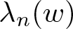 $\lambda_n( w)$ is the
 $n$-th eigenvalue. Let
 $0 \lt \lambda_1 \lt \cdots \lt \lambda_m$ be fixed for an integer
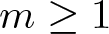 $m\ge 1$ and
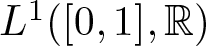 $L^1([0,1],\mathbb{R})$ be the space of real-valued integrable functions. Define
 \begin{equation}
\begin{aligned}
\Omega(\lambda_1,\cdots,\lambda_m)
=\big\{w\in L^1([0,1],\mathbb{R}): w(x)\ge 0,\ \lambda_j(w)=\lambda_j, \ 1\le j\le m \big\}.
\end{aligned}
\end{equation}
We are interested in the infimum of the norm  $\| w\|_1:=\int^1_0|w(x)|{\rm d}x$ for the densities
 $w$ in
 $\Omega(\lambda_1,\cdots,\lambda_m)$, specifically, we search for the quantity
 \begin{equation}
E(\lambda_1,\cdots,\lambda_m):=
\inf\{\| w\|_1:\ w\in\Omega(\lambda_1,\cdots,\lambda_m)\},
\end{equation}
which is termed as the optimal inverse problem for weights [Reference Poschel and Trubowitz13].
For 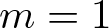 $m=1$, problem (1.5) is equivalently the extremal problem of eigenvalues, which dates back to [Reference Krein10], see also [Reference Barnes1, Reference Egorov and Kondrat’ev6, Reference Ezhak and Telnova7]. A classical example is the Lyapunov inequality, and the optimal weight
 $E(\lambda_1)=4/\lambda_1$ is attained uniquely by the Dirac distribution at
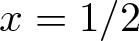 $x=1/2$, as could be found in [Reference Lyapunov11], [Reference Tang and Zhang17, (1.2)], and [Reference Cañada, Montero and Villegas2, p. 177]. There are several tools to study the extremal problems for eigenvalues with separated or coupled boundary conditions, including the Rayleigh–Ritz principle, the variational approach [Reference Chu and Meng3, Reference Chu, Meng and Zhang4], the generalized Lyapunov inequality [Reference Qi and Chen14], and Mercer’s theorem [Reference Qi, Li and Xie15].
When 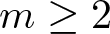 $m\ge 2$, there are few results reported on problem (1.5). The authors of [Reference Ilyasov and Valeev8] and [Reference Zhao and Qi26] studied the optimal potentials in
 $L^2$ and
 $L^1$, respectively. We point out that the optimal inverse problems in
 $L^p$ spaces should be managed distinctively for
 $p=1$ and
 $p \gt 1$ since the latter are reflexive, thereby any bounded subsets of
 $L^p$ for
 $p \gt 1$ are relatively compact. This property ensures that the critical point of problem (1.5) is attainable in such spaces. It is worth noting that the critical point (the optimal weight) of (1.5) may not belong to
 $L^1$, but a larger space, for instance, the measure space, see Section 2 of this paper. For example, the critical point of (1.5) for
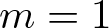 $m=1$ is the Dirac distribution at
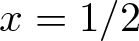 $x=1/2$.
In 2009, the method of critical equations in 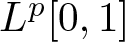 $L^p[0,1]$ for
 $p \gt 1$ was introduced in [Reference Wei, Meng and Zhang20, Reference Zhang25] for Sturm–Liouville operators to study the extremal value problems of eigenvalues in a subset of
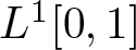 $L^1[0,1]$. Later on, related critical equations were deduced to obtain the optimal lower or upper bounds for eigenvalue gaps of Sturm–Liouville operators in [Reference Tian, Wei and Zhang18]. The critical equations were also established in [Reference Ilyasov and Valeeva9] for elliptic operators. For the inverse problems, the method of critical equations is proved useful as well; for example, it has been adopted in [Reference Qi and Xie16] to obtain the optimal weight of vibrating string equations for
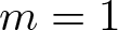 $m=1$.
Generally, it is necessary to solve a boundary value problem with nonlinear differential equations when studying the optimal inverse problems with the method of critical equations, see [Reference Wei, Meng and Zhang20, Reference Zhang25] for 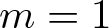 $m=1$ and [Reference Ilyasov and Valeeva9] for
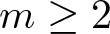 $m\ge 2$. However, the nonlinearity inevitably results in difficulties in solving such boundary value problems directly, especially for the case
 $m\ge 2$.
In the present paper, we are committed to the research of the optimal inverse problem 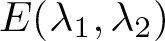 $E(\lambda_1,\lambda_2)$, i.e., problem (1.5) for
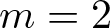 $m=2$. The same problem has been studied in [Reference Qi, Li and Xie15]. By using Mercer’s theorem, it was proved in [Reference Qi, Li and Xie15, Theorem 3.1] that if
 $w(1-x)=w(x)\geq0,a.e.\ x\in(0,1)$ and
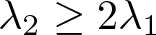 $\lambda_2\geq2\lambda_1$, then
 \begin{equation*}
\int_0^1w(x){\rm d}x\geq \frac{4\lambda_2}{\lambda_1(\lambda_2-\lambda_1)},\ w\in\Omega(\lambda_1,\lambda_2),
\end{equation*}
and the optimal weight can be attained by the Dirac distribution at two points in  $(0,1)$. Almost simultaneously, the authors started pondering whether the condition
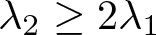 $\lambda_2\geq2\lambda_1$ could be removed or not. On the one hand, they expected that the conclusion would always be true without the condition; on the other hand, they also realized that it might be indispensable. At the end of [Reference Qi, Li and Xie15], several examples ensuring the validity of
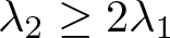 $\lambda_2\geq2\lambda_1$ were displayed and the necessity of the condition was becoming increasingly clear. In the present paper, we improve the result of [Reference Qi, Li and Xie15] and derive the following theorem as the principle conclusion.
Theorem 1.1. Assume that 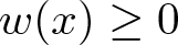 $w(x)\ge 0$ is symmetric on
 $[0,1]$. Then the optimal inverse problem (1.5) for
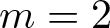 $m=2$ attains its extremum uniquely by the Dirac distribution at two points in
 $(0,1)$ if and only if
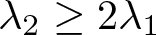 $\lambda_2\geq2\lambda_1$. Furthermore,
 \begin{equation}
E(\lambda_1,\lambda_2)= \frac{4\lambda_2}{\lambda_1(\lambda_2-\lambda_1)}.
\end{equation}
It is worth noting that the method adopted in [Reference Qi, Li and Xie15] does not apply to the proof of necessity of [Reference Qi, Li and Xie15, Theorem 3.1]. We will prove Theorem 1.1 with the method of critical equations. After establishing the critical equations, we do not solve the nonlinear boundary value problem directly but analyse the solution  $w_p$, namely the critical point, in
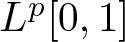 $L^p[0,1]$ to obtain some important properties of the weak limit
 $w_0$ of
 $w_p$ as
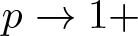 $p\to 1+$ in the measure space. Therefore, the necessary preliminary knowledge for the measure space and the measure differential equations are introduced in Section 2. As an application, we will apply Theorem 1.1 together with Mercer’s theorem to seek the extremum of the partial trace of the first two eigenvalues on a sphere in
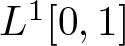 $L^1[0,1]$; both lower and upper bounds are obtained. A similar dual problem for optimal potentials in
 $L^2$ space has been studied in [Reference Valeev and Ilyasov19].
Following this section, Section 2 is devoted to some notations and preliminary results of spectral theory of the vibrating string equation with positive weights in 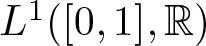 $L^1([0,1],\mathbb{R})$ and the measure space, respectively. In Section 3, we introduce the optimal inverse problem
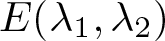 $E(\lambda_1,\lambda_2)$ in
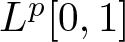 $L^p[0,1]$ for
 $p \gt 1$ and set up the correlative critical equations. We prove Theorem 1.1 in section 4. In Section 5, we apply Theorem 1.1 to study the extremal problem of the partial trace of the first two eigenvalues on a sphere with radius
 $r$ in
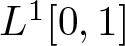 $L^1[0,1]$.
2. Preliminary knowledge of the Sturm–Liouville eigenvalue problems
In this section, we introduce some notations and preliminaries of the vibrating string equation with the Dirichlet boundary condition
 \begin{equation}
-y''(x)=\lambda w(x)y(x),\quad y(0)=0=y(1).
\end{equation}
The weight  $w$ is considered in
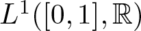 $L^1([0,1],\mathbb{R})$, or more generally, it can be interpreted as
 $\int_{[0,x]}w(s) {\text{d}}s=\mu(x)$ with
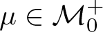 $\mu\in\mathcal{M}^+_{0}$, where the space
 $\mathcal{M}^+_{0}$ is defined later in this section.
Let 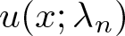 $u(x;\lambda_n)$ be the eigenfunction of (2.1) corresponding to the
 $n$-th eigenvalue
 $\lambda_n=\lambda_n(w)$ satisfying
 \begin{equation}
\int^1_0 |u(x;\lambda_n)|^2 w(x) {\rm d} x=1.
\end{equation}
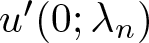
Since  $\lambda_n$ is simple, after fixing the sign of
 $u'(0;\lambda_n)$, such an eigenfunction
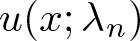 $u(x;\lambda_n)$ is unique, and note that it has exactly
 $n-1$ zero points in (0,1), cf. [Reference Edmunds and Evans5, Reference Zettl23]. Therefore, throughout this paper, we call an eigenfunction
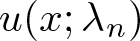 $u(x;\lambda_n)$ of a simple eigenvalue
 $\lambda_n$ is normalized if
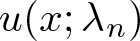 $u(x;\lambda_n)$ satisfies (2.2) and
 $u'(0;\lambda_n) \gt 0$. For problem (2.1), if
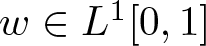 $w\in L^1[0,1]$ and
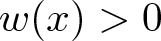 $w(x) \gt 0$ a.e.
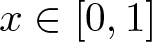 $x\in[0,1]$, then every eigenvalue is simple, and hence the corresponding normalized eigenfunction is well defined.
For other boundary conditions, the normalized eigenfunction can be defined similarly.
The following two lemmas state the continuity and differentiability of eigenvalues with respect to the boundary points and the weights, respectively.
Lemma 2.1. ([Reference Zettl23, p. 54, Theorem 3.5.1; p. 119, Theorem 5.6.1])
Let  $\lambda_n(b)$ be the
 $n$-th eigenvalue of
 \begin{equation}
-y''=\lambda wy,\ \ y=y(x), \ x\in [0,b],\ y(0)=0=y'(b),\ b\in(0,1).
\end{equation}
where  $w\in L^1([0,1],\mathbb{R})$ and
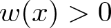 $w(x) \gt 0$ a.e.
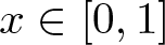 $x\in[0,1]$. Then
(i)  $\lambda_n(b)$ is a continuous function of
 $b$;
(ii) If  $w$ is continuous at
 $b$, then
 $\lambda_n(b)$ is differentiable with respect to
 $b$ and
 \begin{equation}
\lambda_{n}'(b)=-\lambda_{n}(b)w(b)|u_n|^{2}(b),
\end{equation}
where  $u_n(x)$ is the normalized eigenfunction corresponding to
 $\lambda_n(b)$.
Lemma 2.2. ([Reference Zettl23, p. 56])
Let  $w_0\in L^1([0,1],\mathbb{R})$ and
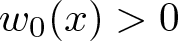 $w_0(x) \gt 0$ a.e.
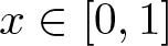 $x\in[0,1]$. Then there exists a neighbourhood
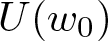 $U(w_0)$ of
 $w_0$ such that for every
 $n\geq1$,
 \begin{equation*}\lambda_n:U\to \mathbb{R},\ w\in U\mapsto \lambda_n(w)\in\mathbb{R}
\end{equation*}
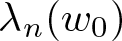
is differentiable at  $w_0$ and its
 $Fr\acute{e}chet$ derivative is given by
 \begin{equation*}
\frac{\partial\lambda_n(w)}{\partial w}{\Big |}_{w=w_0} \cdot h
=-\lambda_n(w_0)\int_0^1 u_n^2(x)h(x){\rm d}x,\ h\in L^1([0,1],\mathbb{R}),
\end{equation*}
where  $u_n(x)$ is the normalized eigenfunction corresponding to
 $\lambda_n(w_0)$.
In order to introduce the spectral theory of (2.1) with measure coefficients, we need to list some basic knowledge of the measure space, see [Reference Chu and Meng3, Reference Wen and Zhou21, Reference Wen, Zhou and Zhang22] for more details. For a real function  $\mu:\ [0,1]\rightarrow \mathbb{R},$ the total variation of
 $\mu$ on
 $[0,1]$ is defined as
 \begin{equation*}\|\mu\|_V=
\sup \left\{\sum\limits_{i=0}\limits^{n-1}|\mu(x_{i+1})-\mu(x_{i})|:\ 0=x_{0} \lt \cdots \lt x_{n}=1,n\in\mathbb{N}\right\}.\end{equation*}
The space of measures on  $[0,1]$ is defined as
 \begin{equation*}
\mathcal{M}_{0}=
\left\{\mu: [0,1]\rightarrow \mathbb{R}: \mu(0+)=0, \mu(x+)=\mu(x), \forall x\in (0,1), \|\mu\|_V \lt \infty\right\},
\end{equation*}
where  $\mu(x+):=\lim_{s\downarrow x}\mu(s),\ x\in [0,1)$ represents the right limit, and the ‘density function’
 $\rho$ is introduced with
 $\int_{[0,x]} \rho(s) {\text{d}}s=\mu(x)$. For example,
 $f\in L^{1}[0,1]$ is the density function of the absolutely continuous measure
 \begin{equation}
\mu_{f}(x):=\int_{[0,x]}f(s){\rm d}s,\ x\in[0,1],
\end{equation}
and the Dirac-Delta function 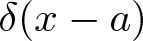 $\delta(x-a)$ at point
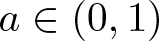 $a\in(0,1)$ is the density function of the Heaviside function
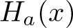 $H_a(x)$, where
 \begin{equation}
H_a(x)=\left\{
\begin{array}{cl}
0, & x\in[0,a), \\
1, & x\in[a,1]. \\
\end{array} \right.
\end{equation}
In the measure space  $\mathcal{M}_{0}$, besides the usual topology induced by the norm
 $\|\cdot\|_V$, there also exists the following weak
 $^{\ast}$ topology, denoted by
 $w^{\ast}$.
Definition 1. Let  $\mu_{n},\ \mu_{0}\in \mathcal{M}_{0},\ n\in \mathbb{N}$.
 $\mu_{n}$ is said to converge weakly
 $^{\ast}$ to
 $\mu_{0}$, denoted as
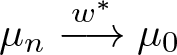 $\mu_{n} \stackrel{w^{\ast}}{\longrightarrow}\mu_{0}$ in
 $(\mathcal{M}_{0},w^{\ast})$, if
 \begin{equation*}\lim\limits_{n\rightarrow\infty}\int_{[0,1]}u(t){\rm d}\mu_{n}(t)=\int_{[0,1]}u(t){\rm d}\mu_{0}(t),\ \forall u\in C[0,1].\end{equation*}
An important property of a subset of 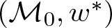 $(\mathcal{M}_0,w^*)$ is proposed below by the Banach–Alaoglu theorem.
Lemma 2.3. A subset  $B\subset(\mathcal{M}_0,w^*)$ is relatively sequentially compact if and only if
 $B$ is norm-bounded in
 $(\mathcal{M}_0,\|\cdot\|_V)$.
Remark 1. (i) Based on the properties of bounded variation functions and the density of the space of absolutely continuous functions in  $(L^{1}[0,1],\|\cdot\|_{1})$, it follows that
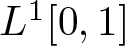 $L^{1}[0,1]$ is dense in
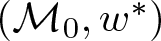 $(\mathcal{M}_{0},w^{\ast})$, that is, for
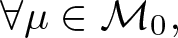 $\forall \mu \in \mathcal{M}_{0},$ there exists
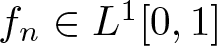 $f_{n}\in L^{1}[0,1]$ such that
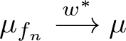 $\mu_{f_{n}}\stackrel{w^{\ast}}{\longrightarrow} \mu$, we also write
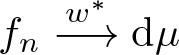 $f_{n}\stackrel{w^{\ast}}{\longrightarrow} {\rm d}\mu$ without any confusion.
(ii) If  $\mu_{n} \stackrel{w^{\ast}}{\longrightarrow}\mu_{0}$ in
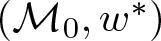 $(\mathcal{M}_{0},w^{\ast})$ and
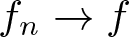 $f_n\to f$ in
 $C[0,1]$, then
 \begin{equation*}
\lim\limits_{n\rightarrow\infty}\int_{[0,1]}f_n(t){\rm d}\mu_{n}(t)=\int_{[0,1]}f(t){\rm d}\mu_{0}(t).
\end{equation*}
(iii) We call 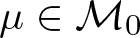 $\mu\in\mathcal{M}_{0}$ a positive measure, denoted by
 $\mu\in\mathcal{M}^+_{0}$, if for all
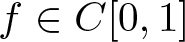 $f\in C[0,1]$ and
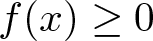 $f(x)\ge 0$, it holds that
 $\int^1_0 f(x){\rm d}\mu(x)\ge 0$. It is easy to verify that if
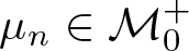 $\mu_n\in\mathcal{M}^+_{0}$ and
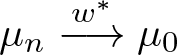 $\mu_{n} \stackrel{w^{\ast}}{\longrightarrow}\mu_{0}$ in
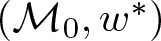 $(\mathcal{M}_{0},w^{\ast})$, then
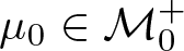 $\mu_0\in\mathcal{M}^+_{0}$.
For 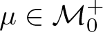 $\mu\in \mathcal{M}^+_{0}$, consider the eigenvalue problem
 \begin{equation}
-{\rm d}\dot{y}(x)=\lambda y {\rm d}\mu(x),\ x\in (0,1), \ y(0)=0=y(1).
\end{equation}
In the present paper, we refer to a specific case of the measure coefficient, explicitly, the density function of  $\mu(x)$ is a Dirac distribution at
 $m$ points on
 $(0,1)$,
 \begin{equation}
\rho(x)=\sum^m_{i=1} r_i\delta(x-x_i),\ r_i \gt 0, x_i\in(0,1),\ 1\le i\le m,\ m\in \mathbb{N},
\end{equation}
and then problem (2.7) can be written in the form of (2.1) as
 \begin{equation}
-y''(x)=\lambda \rho(x) y ,\ x\in (0,1), \ y(0)=0=y(1).
\end{equation}
Compared with (2.1), (2.9) can be particularly a model of the fixed-end vibrating string with  $m$ lumped masses weighting
 $r_i$ attached to it at locations
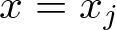 $x=x_j$,
 $1\le i\le m$. Usually, in order to avoid the complexity caused by the Dirac distribution, the boundary problem (2.9) can be interpreted in the sense of
 \begin{equation*}
\left\{\begin{aligned}
&-y''(x)=0,\ x\not=x_i,\ 1\le i\le m, \ y(0)=0=y(1);\\
& y'(x_i-0)-y'(x_i+0)=\lambda r_i y(x_i),\ 1\le i\le m.
\end{aligned}
\right.
\end{equation*}
The following result indicates that the finiteness of the number of eigenvalues for (2.1) implies that the weight must be a Dirac distribution at finite points in  $(0,1)$.
Lemma 2.4. (cf. [Reference Zhang, Wen, Meng, Qi and Xie24])
Consider problem (2.1) with  $\int_{[0,x]}w(s) {\text{d}}s=\mu(x)$,
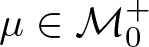 $\mu\in\mathcal{M}^+_{0}$. Then there exist exactly
 $m$ eigenvalues if and only if
 $w$ is a Dirac distribution at
 $m$ points in
 $(0,1)$.
Remark 2. Especially, if  $\rho$ is a Dirac distribution at two points in
 $(0,1)$, being symmetric with respect to
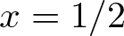 $x=1/2$, that is
 \begin{equation*}
\rho(x)=r\delta(x-a)+r\delta[x-(1-a)],\ r \gt 0,\ 0 \lt a \lt 1/2,
\end{equation*}
then (2.9) has exactly two eigenvalues  $\lambda_1$ and
 $\lambda_2$, and notice that
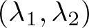 $(\lambda_1, \lambda_2)$ and
 $(r,a)$ are determined uniquely by each other,
 \begin{equation}
\lambda_1=\frac{1}{ra},\ \lambda_2=\frac{1}{ra(1-2a)},
\end{equation}
and
 \begin{equation}
r=\frac{2\lambda_2}{\lambda_1(\lambda_2-\lambda_1)},\
a=\frac{\lambda_2-\lambda_1}{2\lambda_2}.
\end{equation}
Furthermore, the first two eigenfunctions of problem (2.9) are respectively
 \begin{equation}
u(x;\lambda_1)=\left\{
\begin{array}{cl}
\frac{\sqrt{2r}}{2ra} x, & x\in[0,a), \\
\frac{\sqrt{2r}}{2r}, & x\in[a,1-a), \\
\frac{\sqrt{2r}}{2ra} (1-x), & x\in[1-a,1], \\
\end{array} \right.
\end{equation}
and
 \begin{equation}
u(x;\lambda_2)=\left\{
\begin{array}{cl}
\frac{\sqrt{2r}}{2ra} x, & x\in[0,a), \\
\frac{\sqrt{2r}}{2ra-r} (x-\frac{1}{2}), & x\in[a,1-a), \\
\frac{\sqrt{2r}}{2ra} (x-1), & x\in[1-a,1]. \\
\end{array} \right.
\end{equation}
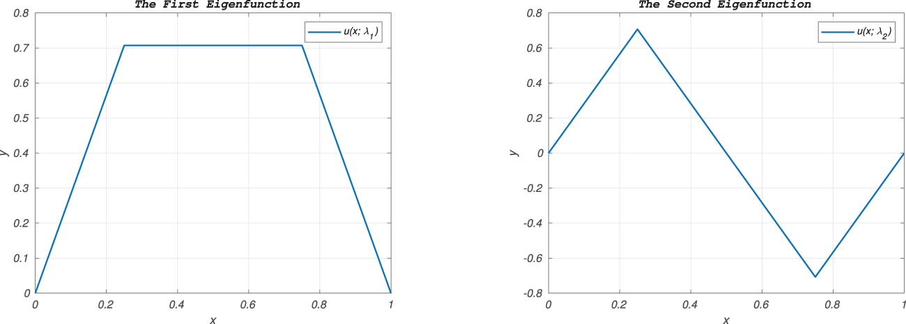
Assuming  $r=1$ and
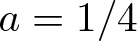 $a=1/4$, then
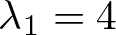 $\lambda_1=4$,
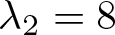 $\lambda_2=8$, their eigenfunctions are plotted in Figure 1 for an intuitive presentation. Evidently, it can be found that
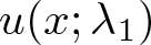 $u(x;\lambda_1)$ of (2.9) is inverted-bathtub-shaped with no zero point in (0,1), and
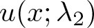 $u(x;\lambda_2)$ has exactly one zero point (1/2,0).
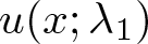 $u(x;\lambda_1)$ and
 $u(x;\lambda_2)$ for r=1 and a=1/4.

It is well known that eigenvalues are continuous on  $w$ with respect to the topology in
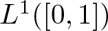 $L^1([0,1])$, see [Reference Zettl23]. Actually, results in [Reference Meng and Zhang12, Reference Zhang, Wen, Meng, Qi and Xie24] show that eigenvalues possess even ‘stronger’ continuity.
Lemma 2.5. (cf. [Reference Zhang, Wen, Meng, Qi and Xie24, Theorem 4.1])
Let 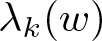 $\lambda_k(w)$ be the
 $k$-th eigenvalue of (2.1) and
 $\phi_{kw}$ be the corresponding normalized eigenfunction for all
 $k\ge 1$. If
 $0\le w_n\in L^1([0,1],\mathbb{R}), n\ge 1$ and
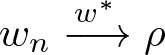 $w_n\xrightarrow[]{w^*} \rho$, where
 $\rho$ is a Dirac distribution at
 $m$ points in
 $(0,1)$, then
 \begin{equation*}
\lambda_k(w_n)\to\lambda_k(\rho),\ \phi_{kw_n}\stackrel{\|.\|_C}{\longrightarrow}\phi_{k\rho}, 1\le k\le m
\end{equation*}
and for  $k\ge m+1$,
 $\lambda_k(w_n)\to\infty$ as
 $n\to\infty$.
Lemma 2.1 and Lemma 2.5 show that eigenvalues are continuous on weights and end points independently, then the following lemma gives the continuity of them jointly in  $(\mathcal{M}_0,w^*)\times \mathbb{R}$.
Lemma 2.6. Let 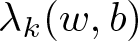 $\lambda_k(w,b)$ be the
 $k$th eigenvalue of
 \begin{equation}
-y''=\lambda wy,\ \ y=y(x), \ x\in [0,b],\ y(0)=0=y'(b), \ b\in(0,1).
\end{equation}
If  $w_n\in C[0,b]$,
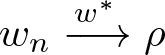 $w_n\xrightarrow[]{w^*} \rho$ and
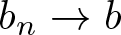 $b_n\to b$ as
 $n\to\infty$, where
 $\rho$ is a Dirac distribution at
 $m$ points in
 $(0,b)$, then
 $\lambda_k(w_n,b_n)\to \lambda_k(\rho, b)$ as
 $n\to\infty$ for
 $1\le k\le m$.
Proof. Let 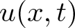 $u(x,t)$ be the associated normalized eigenfunction of (2.14) with
 $b$ replaced by
 $t$. It follows from (ii) of Lemma 2.1 that
 \begin{equation*}
\lambda'(w,t):=\frac{\partial \lambda(w,t)}{\partial t}=-\lambda(w,t)w(t)|u|^{2}(t,t),
\end{equation*}
and hence,
 \begin{equation}
\lambda(w,b_n)-\lambda(w,b)=\int^b_{b_n}\lambda(w,t)w(t)|u|^{2}(t,t)dt.
\end{equation}
Whereas, since  $u(x,t)$ satisfies (2.14) on
 $[0,t]$, write
 $\lambda(w,t)$ as
 $\lambda$, then
 \begin{equation*}\begin{aligned}
u(x,t)&=\lambda\int^x_0\int^t_s w(\tau)u(\tau;t)d\tau ds=\lambda\left(\int^x_0(x-\tau)wu+x\int^t_x wu\right)\\
&=\lambda\left(x\int^t_0w(s)u(s,t)ds-\int^x_0sw(s)u(s,t)ds\right),\ x\in[0,t],
\end{aligned}
\end{equation*}
and hence  $u(t,t)=\lambda\int^t_0(t-s)w(s)u(s,t)ds$, and
 \begin{equation}
\begin{aligned}
|u(t,t)|^2&\le t^2 |\lambda|^2\left(\int^t_0w(s)u(s,t)ds\right)^2\\
&\le t^2 |\lambda|^2\int^t_0 w(s)ds\int^t_0 w(s)u^2(s,t)ds\\
&=t^2 |\lambda|^2\int^t_0 w(s)ds\le b^2|\lambda(w,t)|^2\|w\|_1,
\end{aligned}
\end{equation}
where 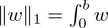 $\|w\|_1=\int^b_0 w$. Since
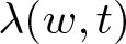 $\lambda(w,t)$ is continuous on
 $t$ by (i) of Lemma 2.1, we have
 $|\lambda(w,t)|\le M$ for
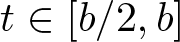 $t\in[b/2,b]$, and hence, (2.15) together with (2.16) yields that
 \begin{equation}
\left|\lambda(w,b_n)-\lambda(w,b)\right|\le b^2M^3\|w\|_1\int^b_{b_n}w(t)dt.
\end{equation}
Since  $\{\|w_n\|_1:\ n\ge 1\}$ is bounded by Lemma 2.3 due to the weak convergence of
 $w_n$, say
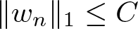 $\|w_n\|_1\le C$, we have from (2.17) that for all
 $n\ge 1$,
 \begin{equation}
|\lambda(w_n,b_n)-\lambda(w_n,b)|\le Cb^2M^3\int^b_{b_n}w_n(t)dt.
\end{equation}
Note that  $w_n\xrightarrow[]{w^*} \rho$ and
 $\rho$ is the Dirac distribution at
 $m$ points in
 $(0,b)$, which implies that
 $\int^b_{b_n}w_n(t)dt\to 0$ as
 $n\to\infty$. As a result, 2.17 yields that
 \begin{equation}
\lambda_k(w_n,b_n)-\lambda_k(w_n,b)\to 0, \ n\to \infty,
\end{equation}
and on the other hand, Lemma 2.5 ensures that for  $1\le k\le m$,
 \begin{equation*}
\lambda_k(w_n,b)-\lambda_k(\rho,b)\to 0, \ n\to \infty.
\end{equation*}
Then we obtain that as  $n\to\infty$,
 \begin{equation*}
\lambda_k(w_n,b_n)-\lambda_k(\rho,b)=\lambda_k(w_n,b_n)-\lambda_k(w_n,b)+\lambda_k(w_n,b)-\lambda_k(\rho,b)\to 0.
\end{equation*}
Remark 3. Checking the proof of Lemma 2.6, it can be detected that for any positive measure 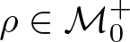 $\rho \in \mathcal{M}^+_{0}$, the conclusion is also valid if
 ${\rm d}\rho(x)$ does not contain the density
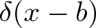 $\delta(x-b)$. In fact, such a restriction is also necessary. See the following example.
Example 2.7. Take  $b=1, b_n=1-1/(2n)$. Let
 \begin{equation*}
w_n(x)=
\left\{\begin{aligned}
& 0,\ x\in[0, 1-1/n],\\
& n \ x\in (1-1/n,1].
\end{aligned}
\right.
\end{equation*}
Clearly  $ w_{n} \stackrel{w^{\ast}}{\longrightarrow} w_{0}=\delta(x-1)$ as
 $n\to\infty$. The eigenvalue problem
 \begin{equation*}
-y''=\lambda w_0 y,\ y(0)=0=y'(1)
\end{equation*}
is equivalent to
 \begin{equation*}
-y''=0,\ y(0)=0=y'(1-0)-\lambda y(1)
\end{equation*}
since  $y'(1-0)-y'(1)=\lambda y(1)$, which means that
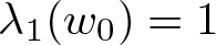 $\lambda_1(w_0)=1$ with the eigenfunction
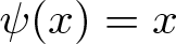 $\psi(x)=x$. Whereas, the first eigenvalue
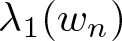 $\lambda_1(w_n)$ of
 \begin{equation*}
-y''=\lambda w_n y,\ y(0)=0=y'(b_n)
\end{equation*}
satisfies
 \begin{equation*}
x\tan x=\frac{1}{2(n-1)},\ x=\frac{\sqrt{n\lambda_1(w_n)}}{2n}.
\end{equation*}
A calculation shows that  $\lambda_1(w_n)\to 2$, as
 $n\to\infty$.
3. The extremal problems and critical equations
In this section, we first introduce the optimal inverse problem  $E_p$ in
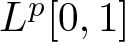 $L^p[0,1]$ for
 $p \gt 1$ associated with the original problem (1.5). Then, we give some properties of critical points and set up the critical equations of
 $E_p$.
We start with the positive and symmetric weights. Here,  $w$ is called
 $\textit{symmetric}$ on
 $[0,1]$ if
 $w(1-x)=w(x),\ a.e.\ x\in[0,1]$. For simplicity,
 $w$ is replaced by
 $\lambda_1 w$ and problem (1.5) reads
 \begin{equation}
\begin{aligned}
&\Omega(\lambda)=\big\{w\in L^1([0,1],\mathbb{R}): \lambda_1(w)=1,\ \lambda_2(w)=\lambda:=\lambda_2/\lambda_1\big\};\\
&E(\lambda)=\inf\left\{\int_0^1 w:\ w\in \Omega(\lambda)\right\}.
\end{aligned}
\end{equation}
That is, 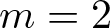 $m=2$ and we always suppose that
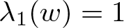 $\lambda_1(w)=1$ and
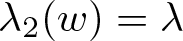 $\lambda_2(w)=\lambda$ in this section. Besides, the infimum
 $E(\lambda)$ is attained by
 $\mu_0$, or
 ${\rm d}\mu_0$, meaning that
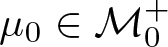 $\mu_0\in\mathcal{M}^+_0$ and
 $\|\mu_0\|_V\le \|w\|_1,\ \forall w\in \Omega(\lambda)$.
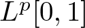
3.1. The associated optimal inverse problems in  $L^P[0,1]$
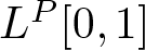
We propose the optimal inverse problems in 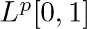 $L^p[0,1]$ for
 $p \gt 1$ associated with problem (3.1). Define
 \begin{equation}
\Omega_p(\lambda)=\{w \in L^p [0,1]:0\le w\in \Omega(\lambda)\ is \ symmetric\},\ p \gt 1,
\end{equation}
and consider the optimal inverse problem
 \begin{equation}
E_p(\lambda)=\inf\left\{\int_0^1 w^p:\ w\in \Omega_p(\lambda)\right\} .
\end{equation}
The existence of the critical point, say  $w_p$, in
 $\Omega_p(\lambda)$ of
 $E_p$ is guaranteed by the results of Eberlein-Smulian theorem since
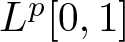 $L^p[0,1]$ is a reflexive space for
 $p \gt 1$. For more details, see [Reference Ilyasov and Valeeva9].
The next lemma indicates that  $\{\|w_p\|_p:\ p \gt 1]\}$ is bounded below.
Lemma 3.1. Let  $w_p$ be a critical point of
 $E_p$ for
 $p \gt 1$. Then
 \begin{equation*}
\|w_p\|_p=\left(\int_0^1 |w_p|^p\right)^{1/p}
\end{equation*}
is bounded below and 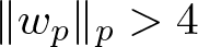 $\|w_p\|_p \gt 4$ for
 $p \gt 1$.
Proof. Since  $L^q[0,1]\subset L^p[0,1]$ if
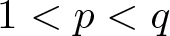 $1 \lt p \lt q$, we have from the definition of
 $w_p$ that
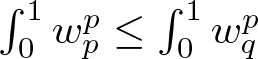 $\int_0^1 w_p^p\leq \int_0^1 w_q^p$, which together with the
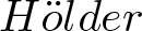 $H\ddot{o}lder$ inequality yields that
 \begin{equation}
\|w_p\|_p=\left(\int_0^1 w_p^p\right)^{1/p}\leq \left(\int_0^1 w_q^p\right)^{1/p}
\leq \left(\int_0^1 w_q^q\right)^{1/q}=\|w_q\|_q.
\end{equation}
3.4 means that 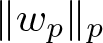 $\|w_p\|_p$ is nondecreasing for
 $p \gt 1$, and hence
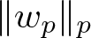 $\|w_p\|_p$ is bounded for
 $p \gt 1$. Moreover, the classical Lyapunov inequality gives that
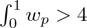 $\int_0^1 w_p \gt 4$, and hence we arrive at
 \begin{equation}
\left(\int_0^1 w_p^p \right)^{1/p} \gt \int_0^1 w_p \gt 4,\ \forall p \gt 1.
\end{equation}
As is proved, the boundedness of 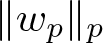 $\|w_p\|_p$ holds for
 $p \gt 1$. However, in the following sections,
 $p$ is always deemed fully close to 1 from the right side. Thus, the conclusion of Lemma 3.1 may actually be utilized on a finite interval, say, for
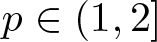 $p \in(1,2]$.
If problem (3.1) attains its extremal value uniquely by a Dirac distribution at two points, then one can verify that this optimal weight must be  $w_0$, see Remark 2, where
 \begin{equation}
w_0=r\delta(x-x_0)+r\delta[x-(1-x_0)],\ r=\frac{2\lambda}{(\lambda-1)},\
x_0=\frac{\lambda-1}{2\lambda}.
\end{equation}
Although whether the critical point  $w_p$ is uniquely determined for each
 $p \gt 1$ remains unclear, we affirm that the critical point
 $w_p$ always has weak limitation as
 $p\to1+$ provided that the infimum
 $E(\lambda)$ is attained uniquely.
Theorem 3.2. Let  $w_p$ be a critical point of (3.3). If the infimum
 $E(\lambda)$ is attained uniquely by
 $w_0$ defined in (3.6), then
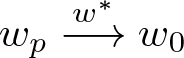 $w_p\stackrel{w^*}{\longrightarrow} w_0$ as
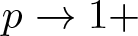 $p\to 1+$.
Proof. We prove the theorem in three steps.
Step 1. There exists  $w^*$-convergent subsequence of
 $w_p$ as
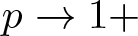 $p\to 1+$. Since for
 $w\in L^1:=L^1([0,1],\mathbb{R})$, the absolute continuous measure
 \begin{equation*}\mu_w(x):=\int_0^x w(s){\rm d}s,\quad x\in[0,1]
\end{equation*}
satisfies  $\| \mu_w\|_V=\|w\|_{L^1}$, we have from Lemma 3.1 that
 $\{\| \mu_{w_p}\|_V: p\in(1,2]\}$ is bounded. Therefore, Lemma 2.3 yields that
 $\mu_{w_{p}}$ has
 $w^*$-convergent subsequence, say,
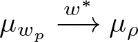 $\mu_{w_p}\stackrel{w^*}{\longrightarrow}\mu_\rho$ for some subsequence of
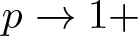 $p\to 1+$ and
 $\mu_\rho\in \mathcal{M}_0^+ $ by (iii) of Remark 1. Taking
 $f\equiv1$, we have from
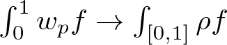 $\int_0^1 w_p f \to \int_{[0,1]} \rho f$ that
 \begin{equation}
\int_0^1 w_{p}(x){\rm d}x \to \int_{[0,1]} \rho(x){\rm d}x:=\|\mu_\rho\|_V
\end{equation}
for some subsequence of  $p\to 1+$.
Step 2. For all 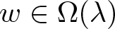 $w\in\Omega(\lambda)$, we claim that
 \begin{equation*}
\int_0^1w(x){\rm d}x\geq \displaystyle\lim_{p\to 1+}\int_0^1 w_p =
\int_{[0,1]} \rho(x){\rm d}x,
\end{equation*}
where 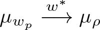 $\mu_{w_{p}}\stackrel{w^*}{\longrightarrow}\mu_\rho$ for some subsequence of
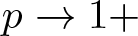 $p\to 1+$. In fact, for
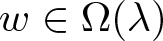 $w\in\Omega(\lambda)$, set
 $A_p=\{x\in[0,1]:\ |w(x)|\leq 1/(p-1)\}$ and introduce
 \begin{equation*}\omega_p(x)=\chi(A_p)(x)w(x),\ x\in[0,1],
\end{equation*}
where 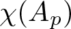 $\chi(A_p)$ is the characteristic function on
 $A_p$. Clearly,
 $\omega_p\to w,\ p\to1+$ in
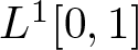 $L^1[0,1]$. Notice that
 $\omega_p\in L^p[0,1]$ for
 $p \gt 1$ and
 $w_{p}$ is a critical point of
 $E_p$, then
 \begin{equation}
\left(\int_0^1 \omega_p^{p}(x){\rm d}x\right)^{1/{p}} \geq
\left(\int_0^1 w_{p}^{p}(x){\rm d}x\right)^{1/{p}}\geq \int_0^1 w_{p}(x){\rm d}x\to \int_{[0,1]} \rho(x){\rm d}x.
\end{equation}
Because
 \begin{equation}
\begin{aligned}
\int_0^1\left|\omega_p^{p}(x)-w(x)\right|{\rm d}x
\leq& \int_0^1 |\omega_p^{p}(x)-\omega_p(x)|{\rm d}x+\int_0^1|\omega_p(x)-w(x)|{\rm d}x\\
=&\int_0^1 \omega_p(x)|\omega_p^{p-1}(x)-1|{\rm d}x+\int_0^1|\omega_p(x)-w(x)|{\rm d}x
\end{aligned}
\end{equation}
By the definition of  $\omega_p(x)$ and
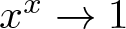 $x^{x}\to 1$ as
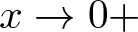 $x\to 0+$, we have
 \begin{equation*}\omega_p(x)|\omega_p^{p-1}(x)-1|\leq \omega_p(x)\left|\left(\frac{1}{p-1}\right)^{p-1}-1\right|\leq
\omega_p(x)\le w(x),\ x\in[0,1]
\end{equation*}
for sufficiently small 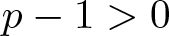 $p-1 \gt 0$. As a result, the dominated convergence theorem ensures that
 \begin{equation*}\int_0^1 \omega_p(x)|\omega_p^{p-1}(x)-1|{\rm d}x\to 0,\ p\to 1+,
\end{equation*}
and hence we have from (3.9) that
 \begin{equation*} \int_0^1\omega_p^{p}(x){\rm d}x\to \int_0^1w(x){\rm d}x,\ p\to 1+.\end{equation*}
Letting  $p\to 1+$ in (3.8), we have
 \begin{equation}
\int_0^1w(x){\rm d}x\geq \int_{[0,1]} \rho(x){\rm d}x,\ \forall w\in\Omega(\lambda).
\end{equation}
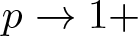
Step 3. We claim that 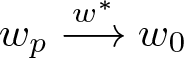 $w_p\stackrel{w^*}{\longrightarrow} w_0$ as
 $p\to 1+$. Since
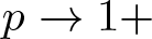
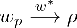 $w_{p}\stackrel{w^*}{\longrightarrow}\rho$ as
 $p\to 1+$, it follows from Lemma 2.5 that
 \begin{equation}
\lambda_1(\rho)=1,\ \lambda_2(\rho)=\lambda.
\end{equation}
Consequently, Step 1 and Step 2 give that 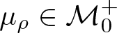 $\mu_\rho\in \mathcal{M}^+_0$ and
 \begin{equation*}
\|\mu_\rho\|_V \leq\inf\left\{\int_0^1w:\ w\in\Omega(\lambda)\right\}.
\end{equation*}
Thus, by the assumption in Theorem 3.2, we know that 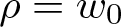 $\rho=w_0$, more specifically,
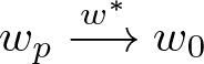 $w_p\stackrel{w^*}{\longrightarrow}w_0$ for all subsequences of
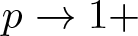 $p\to 1+$.
3.2. The critical equations in
$L^p[0,1]$
In this subsection, we set up the critical equations of problem  $E_p$ for
 $p \gt 1$. Define
 \begin{equation}
F(w,c_1,c_2):=\int_0^1 w^p(x){\rm d}x+c_1[\lambda_1(w)-1]+c_2[\lambda_2(w)-\lambda],
\end{equation}
here  $c_1$ and
 $c_2$ are the Lagrange multipliers for optimizing
 $\int_0^1 w^p(x){\rm d}x$ with the constraints
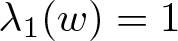 $\lambda_1(w)=1$ and
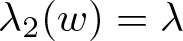 $\lambda_2(w)=\lambda$. Applying Pontryagin’s maximum principle, we know that the critical point
 $w_p$ satisfies
 \begin{equation}
\left\{\begin{aligned}
&\frac{\partial F}{\partial w} (w_p,\hat{c_{1p}},\hat{c_{2p}})=0;\\
&\frac{\partial F}{\partial c_j} (w_p,\hat{c_{1p}},\hat{c_{2p}})=0,\ j=1,2,\\
\end{aligned}
\right.
\end{equation}
for some constants  $\hat{c_{1p}}$ and
 $\hat{c_{2p}}$. To proceed, we adopt the results of Lemma 2.2 and derive that
 \begin{equation}
\left\{\begin{aligned}
&p w_p^{p-1}(x)-\hat{c_{1p}} \lambda_1(w_p) u_{1p}^2(x)-\hat{c_{2p}} \lambda_2(w_p) u_{2p}^2(x)=0;\\
&\lambda_1(w_p)=1,\
\lambda_2(w_p)=\lambda,
\end{aligned}
\right.
\end{equation}
where  $u_{1p}$ and
 $u_{2p}$ are respectively the first and second normalized eigenfunctions of (2.1) given that
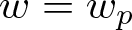 $w=w_p$ and the first two eigenvalues are restricted. Rewriting (3.14) as
 \begin{equation}
pw_p^{p-1}(x)=c_{1p} u_{1p}^2(x)+c_{2p} u_{2p}^2(x),
\end{equation}
where 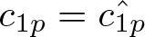 $c_{1p}=\hat{c_{1p}}$,
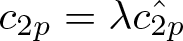 $c_{2p}=\lambda\hat{c_{2p}}$ such that
 $|c_{1p}|+|c_{2p}|\neq 0$, we obtain the following nonlinear boundary value problem
 \begin{equation}
\left\{\begin{aligned}
-&u_{1p}''(x)= w_p u_{1p} (x),\ u_{1p}(0)=0=u_{1p}(1);\\
-&u_{2p}''(x)=\lambda w_p u_{2p} (x),\ u_{2p}(0)=0=u_{2p}(1);\\
&pw_p^{p-1}(x)=c_{1p} u_{1p}^2(x)+c_{2p} u_{2p}^2(x).
\end{aligned}
\right.
\end{equation}
(3.16) is namely the critical equations associated with the optimization problem  $E_p$. The sign of
 $c_{1p}$ and
 $c_{2p}$ in (3.16) is determined in the following theorem.
Theorem 3.3. Let  $w_p$ be a critical point of (3.3). If the infimum
 $E(\lambda)$ is attained uniquely by
 $w_0$ defined in (3.6), then
 $w_p$ satisfies the critical equation (3.16) with
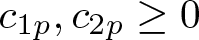 $c_{1p}, c_{2p}\ge 0$ for sufficiently small
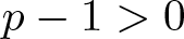 $p-1 \gt 0$.
Proof. Since  $u_{2p}$ has one zero point in
 $(0,1)$ and
 $u_{1p}(x) \gt 0$ on
 $(0,1)$, one sees from (3.15) that
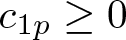 $c_{1p}\ge0$ for all
 $p \gt 1$. We will now prove that
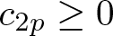 $c_{2p}\ge0$ for sufficiently small
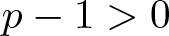 $p-1 \gt 0$.
Suppose on the contrary that there exists a subsequence of 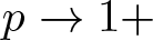 $p\rightarrow 1+$ such that
 $c_{2p} \lt 0$. Then it follows from (3.16) that
 \begin{equation}
w_p^{p-1}(x)=\phi_{1p}^2(x)-\phi_{2p}^2(x),
\end{equation}
with  $\phi_{1p}=\sqrt{c_{1p}/p}\ u_{1p}$ and
 $\phi_{2p}=\sqrt{-c_{2p}/p} u_{2p}$ satisfying
 \begin{equation}
\left\{\begin{aligned}
-&\phi_{1p}''(x)=w_p\phi_{1p}(x),\ \phi_{1p}(0)=0=\phi_{1p}(1),\\
-&\phi_{2p}''(x)=\lambda w_p\phi_{2p}(x),\ \phi_{2p}(0)=0=\phi_{2p}(1).
\end{aligned}
\right.
\end{equation}
Based on the property of  $u_{1p}$ and
 $u_{2p}$, immediately we have
 \begin{equation}
\phi_{1p}'\left(\frac{1}{2}\right)=0=\phi_{2p}\left(\frac{1}{2}\right)
\end{equation}
since the symmetry of  $w_p$ implies that
 $\phi_{1p}(1-x)=\phi_{1p}(x)$,
 $\phi_{2p}(1-x)=-\phi_{2p}(x)$ on
 $[0,1]$.
Multiplying both sides of the first and second equations in (3.18) by
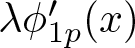 $\lambda\phi_{1p}'(x)$ and
 $\phi_{2p}'(x)$, respectively, and integrating their difference over
 $[0,x]$, we have
 \begin{equation}
\lambda\phi_{1p}'^2(x)-\phi_{2p}'^2(x)+\lambda\frac{p-1}{p} w_p^p(x)\equiv C_p:=\lambda\phi_{1p}'^2(0)-\phi_{2p}'^2(0),
\end{equation}
where the equality (3.17) is used. And then, multiplying both sides of the first and second equations in (3.18) by 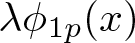 $\lambda\phi_{1p}(x)$ and
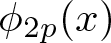 $\phi_{2p}(x)$, respectively, and integrating them on
 $[0,1]$, we have
 \begin{equation*}
\lambda\int_0^1\phi_{1p}'^2=\lambda\int_0^1 w_p\phi_{1p}^2,\ \int_0^1\phi_{2p}'^2=\lambda\int_0^1 w_p\phi_{2p}^2.
\end{equation*}
These equalities together with (3.17) yield that
 \begin{equation}
\int_0^1\left[\lambda\phi_{1p}'^2-\phi_{2p}'^2\right]=\lambda\int_0^1 w_p(\phi_{1p}^2-\phi_{2p}^2)=\lambda\int_0^1 w^p_p.
\end{equation}
Integrating two sides of (3.20) on  $[0,1]$ and using (3.21), we have
 \begin{equation}
C_p=\lambda\left(1+\frac{p-1}{p}\right)\int_0^1 w_p^p=\lambda \frac{2p-1}{p}\int_0^1 w_p^p \gt 0.
\end{equation}
The boundedness of  $\{\|w_p\|_p:\ p\in(1,2]\}$ in Lemma 3.1 implies that
 $C_p$ is bounded for
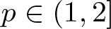 $p\in(1,2]$. Set
 \begin{equation}
\eta_{p}:=\max\{x:\ u_{2p}'(x)=0,\ x\in(0,1/2)\}.
\end{equation}
Then  $\eta_p \lt 1/2$ since
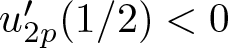 $u'_{2p}(1/2) \lt 0$. This also means that
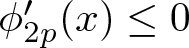 $\phi'_{2p}(x)\le 0$ on
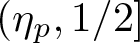 $(\eta_p,1/2]$. Moreover, (3.20) gives that
 \begin{equation*}
\lambda\phi_{1p}'^2(\eta_{p})+\lambda\frac{p-1}{p} w_p^p(\eta_{p})=C_p,
\end{equation*}
and hence 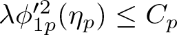 $\lambda\phi_{1p}'^2(\eta_{p})\leq C_p$. Since
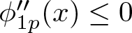 $\phi_{1p}''(x)\le 0$ on
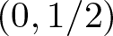 $(0,1/2)$, one sees that
 \begin{equation}
\lambda\phi_{1p}'^2(x)\leq C_p, \ x\in [\eta_p,1/2], \ \forall p \gt 1.
\end{equation}
In order to obtain a contradiction to the assumption that 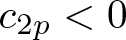 $c_{2p} \lt 0$ for some sequence of
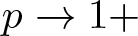 $p\rightarrow 1+$, we carry out the remaining proof in five steps.
Step 1. We assert that  $\eta_{0}=\overline{\lim\limits_{p\to1+}} \eta_{p} \lt 1/2$. Observe that
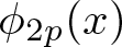 $\phi_{2p}(x)$ is the first eigenfunction of
 \begin{equation*}
-y''(x)=\lambda w_{p}(x)y(x), \ y(0)=0=y'(\eta_{p}),
\end{equation*}
on [0, $\eta_{p}$] with the corresponding eigenvalue
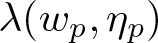 $\lambda(w_p,\eta_{p})$. If
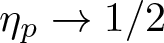 $\eta_{p}\to 1/2$ for some subsequence of
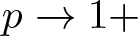 $p\to 1+$, then it follows from Lemma 2.6 that
 $\lambda(w_p,\eta_{p})\to \lambda(w_0,1/2)=\lambda$ jointly, which implies that eigenvalue problems
 \begin{equation*}
-y''=\gamma w_0 y,\ y\left(0\right)=0=y\left(\frac{1}{2}\right)
\end{equation*}
and
 \begin{equation*}
-y''=\gamma w_0 y,\ y\left(0\right)=0=y'\left(\frac{1}{2}\right)
\end{equation*}
have the same first eigenvalue  $\lambda$, where
 $\gamma$ denotes the spectral parameter. Nevertheless, one may find that this cannot be true by calculation, which leads to a contradiction.
Step 2. We declare that for every  $x\in [\eta_{0}, 1/2)$,
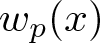 $w_{p}(x)$ is bounded as
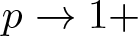 $p\to 1+$. Otherwise, there exists
 $\tilde{x}\in [\eta_{0}, 1/2)$ such that
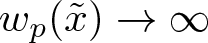 $w_{p}(\tilde{x})\to \infty$ for some subsequence of
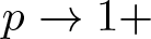 $p\to 1+$. (3.17) yields that
 \begin{equation*}
\frac{1}{2}(w_{p}^{p-1}(x))'=\phi_{1p}'(x)\phi_{1p}(x)-\phi_{2p}'(x)\phi_{2p}(x).
\end{equation*}
Considering the sign of each term obtained previously, we find that  $(w_{p}^{p-1}(x))'\ge 0$, that is,
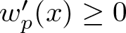 $w'_p(x)\ge 0$ on
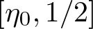 $[\eta_0, 1/2]$, and hence
 \begin{equation*}
\int_{0}^1 w_{p}(t){\rm d}t\geq \int_{\tilde{x}}^{1/2}w_p(t){\rm d}t\geq w_p(\tilde{x})\left(\frac{1}{2}-\tilde{x}\right)\to \infty
\end{equation*}
for some subsequence of 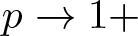 $p\to 1+$, which contradicts the boundedness of
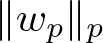 $\|w_p\|_p$ proved in Lemma 3.1.
Step 3. We claim that  $\lambda\phi_{1p}'^2(x)- C_p \to 0$ as
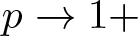 $p\to 1+$ for
 $x\in[\eta_{0}, 1/2)$. If not, by (3.24), we know that there exists
 $\tilde{x}\in[\eta_{0}, 1/2)$ and
 $\varepsilon_0 \gt 0$ such that
 \begin{equation}
\lambda\phi_{1p}'^2(\tilde{x})\leq C_{p}-\varepsilon_0
\end{equation}
for some subsequence of 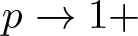 $p\to 1+$. Taking
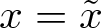 $x=\tilde{x}$ in (3.20) and letting
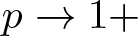 $p\to 1+$ in
 \begin{equation*}\lambda\phi_{1p}'^2(\tilde{x})-\phi_{2p}'^2(\tilde{x})+\lambda\frac{p-1}{p} w_{p}^{p}(\tilde{x})= C_{p},
\end{equation*}
we encounter a contradiction between (3.25) and the conclusion in Step 2.
Step 4. We show that  $\phi_{1p}(1/2)$ is bounded as
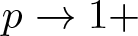 $p\to 1+$. Otherwise, assume that
 $\phi_{1p}(1/2)\to \infty $ for some subsequence of
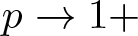 $p\to 1+$. On the one hand, since
 $\phi_{1p}'^2(x)\leq C_p/\lambda$ on
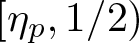 $[\eta_p,1/2)$ as is shown in (3.24) and
 $C_p$ is bounded for
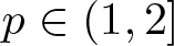 $p\in(1,2]$ in (3.22), we find that
 $\phi_{1p}(\eta_0)\to \infty $ for some subsequence of
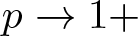
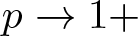 $p\to 1+$. On the other hand, it follows from (3.20), Step 2 and Step 3 that
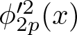 $\phi_{2p}'^2(x)$ is bounded on
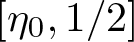 $[\eta_0,1/2]$ as
 $p\to 1+$, and so is
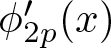 $\phi_{2p}'(x)$. As
 $\phi_{2p}(1/2)=0$ and for some
 $\xi \in (\eta_0,1/2)$
 \begin{equation*}
\phi_{2p}\left(\frac{1}{2}\right)-\phi_{2p}\left(\eta_0\right)=\phi'_{2p}(\xi)\left(\frac{1}{2}-\eta_0\right),
\end{equation*}
we know that 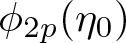 $\phi_{2p}(\eta_0)$ is bounded as
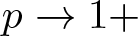 $p\to 1+$. Finally, by (3.17), we derive that
 \begin{equation*}
w_p^{p-1}(\eta_0)=\phi_{1p}^2(\eta_0)-\phi_{2p}^2(\eta_0)\to \infty
\end{equation*}
for some subsequence of 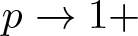 $p\to 1+$, and hence
 $w_p(\eta_0)\to \infty$ accordingly, which contradicts the conclusion in Step 2.
Step 5. Set  $\alpha_p=\phi_{1p}'(0), \ \beta_p=\phi_{2p}'(0)$. Since
 \begin{equation*}
\phi_{1p}\left(\frac{1}{2}\right)=\frac{\alpha_p}{2}-\int^{1/2}_0\left(\frac{1}{2}-t\right)w_p(t)\phi_{1p}(t) dt,
\end{equation*}
we have
 \begin{equation*}
\left|\alpha_p\right|\le \left|\phi_{1p}\left(\frac{1}{2}\right)\right|\left(2+\int^{1/2}_0|w_p(t) dt|\right),
\end{equation*}
and hence  $\alpha_p$ is bounded as
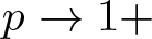 $p\to 1+$ by the boundedness of
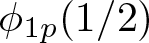 $\phi_{1p}(1/2)$ and
 $\|w_p\|$. As discussed earlier,
 $C_p$ is bounded, and therefore by (3.20),
 $\beta_p^2=\lambda\alpha_p^2-C_p$ is surely bounded as
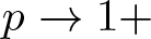 $p\to 1+$.
Subsequently, set 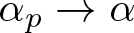 $\alpha_p\to\alpha$ and
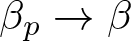 $\beta_p\to\beta$ for some subsequence of
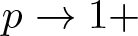 $p\to 1+$. Since
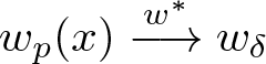 $w_{p}(x)\stackrel{w^*}{\longrightarrow} w_\delta $, it follows from Lemma 2.5 that as
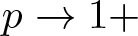 $p\to 1+$,
 \begin{equation*}
\phi_{1p}\to \phi_1,\ \phi_{2p}\to \phi_2
\end{equation*}
uniformly on 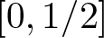 $[0,1/2]$, where
 $\phi_1$ and
 $\phi_2$ are respectively the first and second eigenfunctions of
 $-y''=\mu w_0 y, \ y(0)=0=y(1)$ such that
 $\phi_1'(0)=\alpha$ and
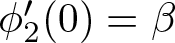 $\phi_2'(0)=\beta$, namely,
 \begin{align}
\begin{array}{cl}
&\phi_1(x)=\left\{
\begin{array}{cl}
\alpha x, & x\in[0,x_0], \\
\alpha x_0, & x\in[x_0,1/2], \\
\end{array} \right.\nonumber\\
& \phi_2(x)=\left\{
\begin{array}{cl}
\beta x, & x\in[0,x_0], \\
\beta(\lambda-1)(\frac{1}{2}-x), & x\in[x_0,1/2], \\
\end{array} \right.
\end{array}
\end{align}
where 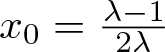 $x_0=\frac{\lambda-1}{2\lambda}$. Since
 $w_p^{p-1}(x)=\phi_{1p}^2(x)-\phi_{2p}^2(x)$ and
 $\phi_{1p}$,
 $\phi_{2p}$ converge to
 $\phi_{1}$,
 $\phi_{2}$ uniformly on
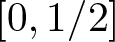 $[0,1/2]$, respectively, applying the expression of
 $\phi_{1}$ and
 $\phi_{2}$ in (3.26), one may verify that
 $w_p^{p-1}(x_1) \lt w_p^{p-1}(x_2)$, or equivalently,
 $w_p(x_1) \lt w_p(x_2)$ for
 $0\le x_1 \lt x_2\le 1/2$ and
 $p$ sufficiently close to the right of 1. Moreover,
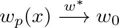 $w_{p}(x)\stackrel{w^*}{\longrightarrow} w_0$ implies that
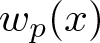 $w_p(x)$ is unbounded in every neighbourhood
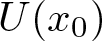 $U(x_0)$ of
 $x_0$ as
 $p\to1+$, it follows that
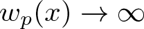 $w_p(x)\to \infty$ as
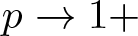 $p\to 1+$ on
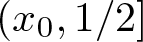 $(x_0,1/2]$, which clearly contradicts the conclusion in Step 2. Hence, Theorem 3.3 is proved.
From now on (3.15) takes the form
 \begin{equation}
w_p^{p-1}(x)=\phi_{1p}^2(x)+\phi_{2p}^2(x),
\end{equation}
where  $\phi_{1p}=\sqrt{c_{1p}/p} u_{1p},\ \phi_{2p}=\sqrt{c_{2p}/p} u_{2p}$, and they satisfy (3.18). Then
 \begin{equation}
\lambda\phi_{1p}''(x)\phi_{1p}'(x)-\phi_{2p}''(x)\phi_{2p}'(x)+\lambda w_p(\phi_{1p}(x)\phi_{1p}'(x)-\phi_{2p}(x)\phi_{2p}'(x))=0.
\end{equation}
Integrating (3.28) on  $[0,x]$, we have
 \begin{equation}
\lambda\phi_{1p}'^2(x)+\phi_{2p}'^2(x)+\lambda\frac{p-1}{p} w_p^p(x)\equiv C_p:=\lambda\phi_{1p}'^2(0)+\phi_{2p}'^2(0).
\end{equation}
We call (3.29) the first integral associated with the critical equation (3.27). Similarly as before, we have from (3.28) that
 \begin{equation}
\lambda\int_0^1\phi_{1p}'^2=\lambda\int_0^1 w_p\phi_{1p}^2,\ \int_0^1\phi_{2p}'^2=\lambda\int_0^1 w_p\phi_{2p}^2,
\end{equation}
and hence
 \begin{equation}
\int_0^1\left[\lambda\phi_{1p}'^2+\phi_{2p}'^2\right]=\lambda\int_0^1\left[w_p(\phi_{1p}^2+\phi_{2p}^2)\right].
\end{equation}
Integrating (3.29) on  $[0,1]$ and employing (3.31), we have
 \begin{equation}
C_p=\lambda\left(1+\frac{p-1}{p}\right)\int_0^1 w_p^p(x)=\lambda \frac{2p-1}{p}\int_0^1 w_p^p(x).
\end{equation}
Evidently, it can be seen from (3.32) that  $C_p$ is bounded for
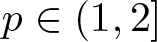 $p\in(1,2]$ due to the boundedness of
 $\|w_p\|$ by Lemma 3.1.
4. The proof of Theorem 1.1
In this section, we will use the critical equation (3.27) and the first integral (3.29) to prove Theorem 1.1. We begin with the following lemma in consideration of the boundedness of  $C_p$ in (3.32).
Lemma 4.1. Suppose that all the assumptions in Theorem 3.3 are satisfied. Let  $\phi_{1p}$ and
 $\phi_{2p}$ be defined as in (3.27). Then the set
 \begin{equation*}
\{\phi_{1p}(x),\phi_{1p}'(x),\phi_{2p}(x),\phi_{2p}'(x):x\in[0,1],p\in(1,2]\}
\end{equation*}
is bounded.
Proof. Since  $C_p=\lambda\phi_{1p}'^2(0)+\phi_{2p}'^2(0)$ is bounded, both
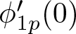 $\phi_{1p}'(0)$ and
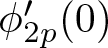 $\phi_{2p}'(0)$ are bounded for
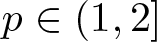 $p\in(1,2]$. Furthermore, we get from
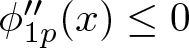 $\phi_{1p}''(x)\le 0$ and
 $\phi_{1p}'(x)(1/2-x)\ge 0$ that
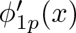 $\phi_{1p}'(x)$ is bounded on
 $[0,1]$ for
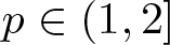 $p\in(1,2]$. Therefore,
 $\phi_{1p}(x)=\int_{0}^x\phi_{1p}'(t){\rm d}t$ gives that
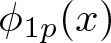 $\phi_{1p}(x)$ is bounded on
 $[0,1]$ for
 $p\in(1,2]$. Similarly, the boundedness of
 $\phi_{2p}(x)$ and
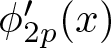 $\phi_{2p}'(x)$ can be proved on
 $[0,1]$ for
 $p\in(1,2]$.
Let  $\phi_{1p}$ and
 $\phi_{2p}$ be defined as in (3.27). Lemma 4.1 implies that
 $\phi_{1p}$ and
 $\phi_{2p}$ respectively converge to
 $\phi_1$ and
 $\phi_2$ as
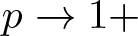 $p\to 1+$ uniformly on
 $[0,1]$, where
 $\phi_1$ and
 $\phi_2$, as shown in (3.26), are the first and second eigenfunctions of
 $-y''=\mu w_0 y, \ y(0)=0=y(1)$ such that
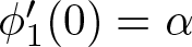 $\phi_1'(0)=\alpha$ and
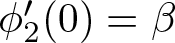 $\phi_2'(0)=\beta$, with
 $\alpha$ and
 $\beta$ given by
 \begin{equation}
\phi'_{1p}(0)\to \alpha,\ \phi'_{2p}(0)\to \beta,\ p\to1+.
\end{equation}
Lemma 4.2. Suppose that all the assumptions in Theorem 3.3 are satisfied. Let  $w_p$ be a critical point of
 $E_p$, and
 $\phi_1(x),\ \phi_2(x)$ be defined as in (3.26). Then the following properties hold.
(i)  $(\alpha^2 + \beta^2)x_0^2=1$;
(ii)  $\beta\not=0$;
(iii) There exists  $\delta \gt 0$, s.t.
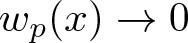 $w_p(x)\to 0$ as
 $p\to 1+$ uniformly on
 $[1/2-\delta, 1/2+\delta]$.
Proof. (i) Suppose on the contrary that there exists  $\varepsilon_0 \gt 0$ such that
 \begin{equation*}
\left|(\alpha^2 + \beta^2)x_0^2-1\right|\ge 2\varepsilon_0.
\end{equation*}
Without loss of generality, we assume that  $(\alpha^2 + \beta^2)x_0^2\ge 1+2\varepsilon_0$. By the continuity of
 $\phi_1(x)$,
 $\phi_2(x)$ and the uniform convergence of
 $\phi_{jp}$(
 $j=1,2$) on
 $[0,1]$ as
 $p\to 1+$, there exists
 $\delta \gt 0$ such that for sufficiently small
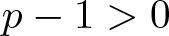 $p-1 \gt 0$,
 \begin{equation*}
\phi^2_{1p}(x)+\phi^2_{2p}(x)\geq1+\varepsilon_0. \quad x_0-\delta \lt x \lt x_0+\delta.
\end{equation*}
Then the critical equation (3.27) yields that  $(w_p(x))^{p-1} \geq 1+\varepsilon_0$ on
 $[x_0-\delta, x_0+\delta]$, and hence
 \begin{equation*}
\int^{x_0+\delta}_{x_0-\delta} w_p(x){\rm d}x \geq 2\delta(1+\varepsilon_0)^{\frac{1}{p-1}} \rightarrow+\infty,\ p\to1+,
\end{equation*}
which contradicts Lemma 3.1.
(ii) Note that (3.32) implies that
 \begin{equation*}
C_p=\lambda \frac{2p-1}{p}\int_0^1 w_p^p(x)\to 2r\lambda,\ r=\frac{2\lambda}{\lambda-1}(see \ 3.6).
\end{equation*}
Whereas, the definition of  $C_p$ in (3.29) together with (4.1) gives that
 \begin{equation*}
C_p=\lambda \phi'_{1p}(0)+\phi'_{1p}(0)\to \lambda\alpha^2+\beta^2,\ p\to 1+.
\end{equation*}
Then  $2r\lambda=\lambda\alpha^2+\beta^2$, and hence
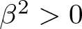 $\beta^2 \gt 0$ by
 $(\alpha^2 + \beta^2)x_0^2=1$ and
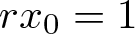 $rx_0=1$.
(iii) Considering that  $\beta\not=0$, we have that
 \begin{equation*}\alpha^2x_0^2 \lt (\alpha^2+\beta^2)x_0^2=1.
\end{equation*}
Set  $\alpha^2x_0^2 = 1-2\varepsilon _1$. By the continuity of
 $\phi _1^2(x)+\phi_2^2(x)$ at
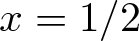 $x=1/2$ and the uniform convergence of
 $\phi_{jp}$(
 $j=1,2$), there exists
 $\delta \gt 0$ such that
 \begin{equation*}
\phi^2_{1p}(x)+\phi^2_{2p}(x)\leq 1-\varepsilon_1, \ |x-1/2|\le \delta
\end{equation*}
for sufficiently small 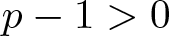 $p-1 \gt 0$, and hence
 $w_p(x) \leq (1-\varepsilon_1)^{\frac{1}{p-1}} \rightarrow 0,\ p\to1+.$
Now, we proceed to prove the main result of this paper, Theorem 1.1, with the aid of Lemma 4.1 and Lemma 4.2.
The proof of Theorem 1.1
 $\Rightarrow$) Suppose that the problem (3.1) attains its optimal weight uniquely by a Dirac distribution at two points. Then a calculation gives that
 $w_0$ defined as in (3.6) is the unique optimal weight. Let
 $w_p$,
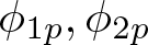 $\phi_{1p}, \phi_{2p}$ and
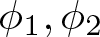 $\phi_1,\phi_2$ be defined as before. Lemma 4.1 and Lemma 4.2 yield that
 $C_p=\lambda\phi_{1p}'^2(0)+\phi_{2p}'^2(0)\to \lambda\alpha^2+\beta^2$ as
 $p\to 1+.$ On the other hand, as
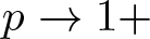 $p\to 1+$, since
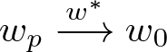 $w_{p}\stackrel{w^*}{\longrightarrow} w_0$, based on the uniform convergence of
 $\phi_{2p}$, we obtain
 \begin{equation}
\phi_{2p}'(0)-\phi_{2p}'(1/2)=\lambda \int^{1/2}_0 w_p \phi_{2p}\to
\lambda\int_{[0,1/2]} w_0 \phi_2=\lambda r\beta x_0=\beta\lambda.
\end{equation}
(4.2) together with  $\phi_{2p}'(0)=\beta_p\to\beta$, see (4.1), guarantees that
 $\phi_{2p}'(1/2)\to \beta(1-\lambda)$ as
 $p\to 1+$.
Set 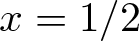 $x=1/2$ in (3.29). We have
 \begin{equation}
\phi_{2p}'^2(1/2)+\lambda\frac{p-1}{p} w_p^p(1/2)=C_p:=\lambda\phi_{1p}'^2(0)+\phi_{2p}'^2(0)
\end{equation}
since 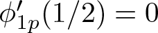 $\phi_{1p}'(1/2)=0$. Letting
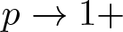 $p\to1+$ in (4.3), it follows from
 $w_p(1/2)\to 0$, (4.1) and (4.2) that
 \begin{equation*}
\lambda\alpha^2+\beta^2=\beta^2(\lambda-1)^2,
\end{equation*}
which means that  $\lambda\geq 2.$ A calculation gives that
 \begin{equation*}
\int_0^1 w_0=2r=\frac{4\lambda}{\lambda-1}.
\end{equation*}
Recover the original form, we have proven that  $\lambda_2\ge 2\lambda_1$ and
 \begin{equation*}
E(\lambda_1,\lambda_2)=\frac{4\lambda_2}{\lambda_1(\lambda_2-\lambda_1)}.
\end{equation*}
 $\Leftarrow$) Suppose that
 $\lambda_2\geq 2\lambda_1$. The optimal weight
 $w_0$ has been illustrated in Theorem 3.1 of [Reference Qi, Li and Xie15]; we only need to prove that
 $w_0$ is unique herein. For the sake of completeness, we provide both the proof of existence and uniqueness since some inequalities in the proof of existence will be used later.
It follows from Corollary 3.2 in [Reference Qi, Li and Xie15] that
 \begin{equation}
\int_0^1 w(x){\rm d}x\geq \frac{4\sigma_1^2}{\sigma_1-\sigma_2}, \ \sigma_1=\sum_{j=1}^{\infty}\frac{1}{\lambda_{2j-1}},\
\sigma_2=\sum_{j=1}^{\infty}\frac{1}{\lambda_{2j}}.
\end{equation}
Set  $\sigma_1=t/\lambda_1,\ \sigma_2=s/\lambda_2$. Then
 $s,\ t\in [1,+\infty)$ and (4.4) gives
 \begin{equation}
\int_0^1w(x){\rm d}x\geq \frac{4t^2\lambda_2}{\lambda_1(t\lambda_2-s\lambda_1)}.
\end{equation}
Since  $\lambda_2\ge 2\lambda_1$, we have
 \begin{equation*}
(t^2-t)\lambda_2\ge 2(t^2-t)\lambda_1=(t-1)^2\lambda_1+(t^2-s)\lambda_1+(s-1)\lambda_1
\ge(t^2-s)\lambda_1,
\end{equation*}
which means that
 \begin{equation}
\frac{4t^2\lambda_2}{\lambda_1(t\lambda_2-s\lambda_1)}\geq\frac{4\lambda_2}{\lambda_1(\lambda_2-\lambda_1)},
\end{equation}
and hence
 \begin{equation*}E(\lambda_1,\lambda_2)\ge \frac{4\lambda_2}{\lambda_1(\lambda_2-\lambda_1)}.
\end{equation*}
Let  $w_0$ be defined as in (3.6). Then the ‘
 $=$’ holds in the above equality.
It remains to prove that the optimal weight is attained uniquely by  $w_0$. That is, if
 $\lambda_1(\hat{w})=\lambda_1, \lambda_2(\hat{w})=\lambda_2$ and
 \begin{equation*}
\int_0^1 \hat{w} {\rm d}x= \frac{4\lambda_2}{\lambda_1(\lambda_2-\lambda_1)},
\end{equation*}
then 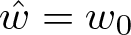 $\hat{w}=w_0$. Let
 $\sigma_1$ and
 $\sigma_2$ be defined as (4.4) and set
 \begin{equation*}
\hat{t}=\lambda_1\sigma_1,\ \hat{s}=\lambda_2\sigma_2.
\end{equation*}
Then  $\hat{t}, \hat{s}\in[1,\infty)$ and it follows from (4.5) that
 \begin{equation}
\int_0^1 \hat{w}{\rm d}x\geq \frac{4\hat{t}^2\lambda_2}{\lambda_1(\hat{t}\lambda_2-\hat{s}\lambda_1)}.
\end{equation}
Therefore, (4.6) together with (4.7) means that
 \begin{equation}
\frac{4\hat{t}^2\lambda_2}{\lambda_1(\hat{t}\lambda_2\hat{s}-\lambda_1)}=\frac{4\lambda_2}{\lambda_1(\lambda_2-\lambda_1)}, \ or \ \frac{\hat{t}^2}{\hat{t}\lambda_2-\hat{s}\lambda_1}= \frac{1}{\lambda_1(\lambda_2-\lambda_1)}.
\end{equation}
This also means that
 \begin{equation}
(\hat{t}^2-\hat{t})\lambda_2= (\hat{t}^2-\hat{s})\lambda_1.
\end{equation}
On the other hand, since  $\lambda_2\geq 2\lambda_1 \gt 0$ and
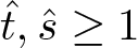 $\hat{t},\hat{s}\ge 1$, we have from
 \begin{equation*}
(\hat{t}^2-\hat{s})\lambda_1=(\hat{t}^2-\hat{t})\lambda_2\geq 2(\hat{t}^2-\hat{t})\lambda_1=(\hat{t}-1)^2\lambda_1+(\hat{t}^2-\hat{s})\lambda_1+(\hat{s}-1)\lambda_1
\end{equation*}
that 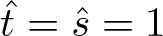 $\hat{t}=\hat{s}=1$. This implies that (2.1) has exactly two eigenvalues, and hence Lemma 2.4 implies that the weight must be the Dirac distribution at two points and a calculation gives that the weight is
 $w_0$ as defined in (3.6).
Remark 4. Theorem 1.1 presents a necessary and sufficient condition for optimal inverse problem (1.5) as 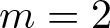 $m=2$, which improves the result in [Reference Qi, Li and Xie15] by filling in the necessity of the conclusion. In particular, the necessity here signifies that for (1.5), if its extremum is attained uniquely by the Dirac distribution at two points in
 $(0,1)$, then
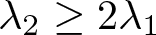 $\lambda_2\geq2\lambda_1$. As noted in Remark 1 of [Reference Qi, Li and Xie15], it is expected that Corollary 3.4 therein could be proved without the extra condition
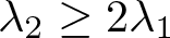 $\lambda_2\geq2\lambda_1$. Based on the conclusion obtained in the present paper, if such a restriction is removed, then the optimal weight function would not be a Dirac distribution at two points on (0,1), but more complex. Intuitively, we conjecture that it may be a Dirac distribution at more than two points.
5. The extremal problem for partial trace
In this section, as an application, we study the extremal problem for partial trace of the first two eigenvalues associated with (2.1), i.e.,
 \begin{equation}
-y''(x)=\lambda w(x)y(x),\quad y(0)=0=y(1),
\end{equation}
where  $w\in B_r^+\subset L^1([0,1],\mathbb{R})$,
 \begin{equation*}
B_r^+=\{w\in L^1([0,1],\mathbb{R}):\ \|w\|_1=r, \ w(x)\ge 0, a.e. x\in[0,1]\}.
\end{equation*}
We search for the infimum of the set  $V(r)$, where
 \begin{equation}
V(r)=\{\lambda_1(w)+\lambda_2(w):\ w\in B_r^+\},\ r \gt 0,
\end{equation}
with 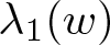 $\lambda_1(w)$ and
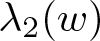 $\lambda_2(w)$ being respectively the first and second eigenvalues of (5.1). Introduce
 \begin{equation}
B_r^+(s)=\{w\in B_r^+: \ \lambda_2(w)\ge 2\lambda_1(w),\ w(x)=w(1-x), x\in[0,1]\}.
\end{equation}
Note that 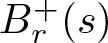 $B_r^+(s)$ is not empty by Remark 2 in Section 1 for
 $a\in[1/4,1/2)$. Clearly,
 $B_r^+(s)\subset B_r^+$, and hence
 $\inf V(r)\le \inf V(r,s)$, where
 \begin{equation}
V(r,s)=\{\lambda_1(w)+\lambda_2(w):\ w\in B_r^+(s)\}.
\end{equation}
Fix 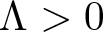 $\Lambda \gt 0$, set
 \begin{equation}
\begin{aligned}
\Omega(\Lambda)=&\big\{w\in L^1([0,1],\mathbb{R}): \lambda_1(w)+\lambda_2(w)=\Lambda, \ \lambda_2(w)\ge 2\lambda_1(w)\\
& 0\le w,\ w(x)=w(1-x), x\in[0,1]\big\};\\
E(\Lambda)=&\inf\left\{\|w\|_1:\ w\in \Omega(\Lambda)\right\}.
\end{aligned}
\end{equation}
Then the dual problem of 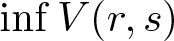 $\inf V(r,s)$ is just problem
 $E(\Lambda)$ for weights. That is, if
 $r=E(\Lambda)=f(\Lambda)$, then
 $\Lambda=\inf V(r,s)=f^{-1}(r)$, where
 $f^{-1}$ is the inverse function of
 $f$. Similar problems of
 $ E(\Lambda)$ in
 $L^2$ space for optimal potential of
 \begin{equation*}
-y''+qy=\lambda y,\ y(0)=0=y(1)
\end{equation*}
has been studied in [Reference Valeev and Ilyasov19, Theorems 1.1 and 1.2] and the existence and uniqueness of the optimal potential are established.
For given  $\lambda_1, \lambda_2$ such that
 $0 \lt 2\lambda_1\le\lambda_2$ and
 $\lambda_1+\lambda_2=\Lambda$, we set
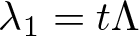 $\lambda_1=t\Lambda$ and
 $\lambda_2=(1-t)\Lambda$ for
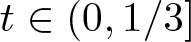 $t\in(0,1/3]$. See (1.6), the definition of
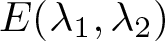 $E(\lambda_1,\lambda_2)$) for
 $w\in\Omega(\Lambda)$ and
 $\lambda_1(w)=\lambda_1, \lambda_2(w)=\lambda_2$ reads
 \begin{equation*}
E(\lambda_1,\lambda_2)=\frac{4\lambda_2}{\lambda_1(\lambda_2-\lambda_1)}=\frac{4}{\Lambda}\frac{1-t}{t(1-2t)}:=H(t),\ t\in(0,1/3].
\end{equation*}
A calculation gives that the minimal value of  $H(t)$ on
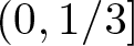 $(0,1/3]$ is attained by
 \begin{equation*}
H_{min}=H(a)=\frac{4}{\Lambda}(1+\sqrt{2})^2,\ a=1/(2+\sqrt{2}).
\end{equation*}
Therefore,  $E(\Lambda)=H(a)$, which also means that
 \begin{equation}
\inf V(r,s)=\frac{4}{r}(1+\sqrt{2})^2\ge \inf V(r).
\end{equation}
(5.6) offers an upper bound of 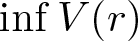 $\inf V(r)$. Now, we apply Mercer’s theorem to find a lower bound. According to Lemma 2.4 in [Reference Qi and Xie16],
 \begin{equation*}
\int^1_0G(x,x) w(x){\text{d} x}=\sum^\infty_{n=1}\frac{1}{\lambda_n(w)}
\ge \frac{1}{\lambda_1}+\frac{1}{\lambda_2}=\frac{\lambda_1+\lambda_2}{\lambda_2\lambda_1},
\end{equation*}
where 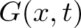 $G(x,t)$ is the Green function of
 $-y''=0$ with
 $y(0)=0=y(1)$, and hence
 $G(x,x)=x(1-x)$ on
 $[0,1]$. Set
 $\Lambda=\lambda_1+\lambda_2$,
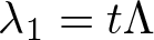 $\lambda_1=t\Lambda$, and
 $\lambda_2=(1-t)\Lambda$ for
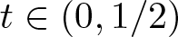 $t\in(0,1/2)$. Then
 \begin{equation*}
r=\int^1_0 w(x){\text{d} x}\ge \frac{4}{\Lambda t(1-t)} \gt \frac{16}{\Lambda},\ t\in(0,1/2)\Rightarrow
\Lambda \gt \frac{16}{r}.
\end{equation*}
In fact, the next theorem readily follows the above discussion.


Acknowledgements
This work was supported by the Natural Science Foundation of Shandong Province (ZR2024MA005) and the National Natural Science Foundation of China (Grants 12271299 and 12071254). The authors would like to express their sincere gratitude to the anonymous referees for their constructive criticism and helpful suggestions.