1 INTRODUCTION
Heterogeneity is a fundamental feature in many economic datasets and how to model heterogeneity has been a central issue in econometrics (see, e.g., Heckman, Reference Heckman2001). In this article, we propose a linear panel data model with a general form of heterogeneity. In our model, the outcome variable depends on both observable covariates and unobservable factors in a heterogeneous way. The slope coefficients of covariates are allowed to vary along both cross-sectional and time-series dimensions. We also allow multiple latent common factors (i.e., interactive fixed effects [IFEs hereafter]) to affect the outcome variable via an intercept term. Our model nests many commonly used panel data models as special cases, such as the homogeneous panel data model with IFEs, the random coefficient model, the time-varying coefficient model, and the panel data model with two-dimensional heterogeneity, among others (for details, see the literature review below). We propose estimation and inference methods for our heterogeneous model. One important application of our model is to estimate the counterfactual outcomes for program evaluations.
An important feature of our model is that it allows the observable covariates,
$x_{it}$
 , to influence the outcome heterogeneously, varying across both individuals and time. The importance of allowing heterogeneous effects has been well recognized in panel data models, and the homogeneous slope coefficients are often rejected empirically (see, e.g., Browning and Carro, Reference Browning and Carro2007; Su and Chen, Reference Su and Chen2013). As we estimate all the slope coefficients,
$\beta _{i\cdot }^{0}$
 and
$\beta _{\cdot t}^{0},$
 it is transparent to examine the role of covariates in explaining the outcome. To illustrate the importance of allowing for heterogeneous slopes, consider the famous Feldstein–Horioka puzzle in international economics (see, e.g., Feldstein and Horioka, Reference Feldstein and Horioka1980), where
$y_{it}$
 and
$x_{it}$
 are the investment rate and saving rate for country i in year
$t,$
 respectively. The standard economic theory suggests that rational investors would invest in countries offering the highest return if there were no regulations in international financial markets. However, in practice, investors may face all kinds of regulations in investing in foreign countries. Therefore, the effect of domestic saving rates on investment rates depends on the constraints of capital mobility across countries. Based on this argument, the slope coefficient (
$\beta _{it}^{0}$
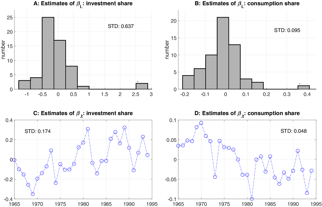
 ) of saving rates should be country-specific. It should also be time-varying, as the international capital market environments change over time. Lu and Su (Reference Lu and Su2023) find strong evidence of heterogeneity in both dimensions using a simpler model that does not incorporate a factor structure. In our empirical study in Section 6, where we investigate the relationship between countries’ economic growth and their consumption and investment shares, we also find substantial heterogeneity in the effects of these two variables on growth (see Figure 1 in Section 6). As Lu and Su (Reference Lu and Su2023) argue, neglecting heterogeneity in slope coefficients can result in model misspecification and undermine the validity of subsequent estimation and inference in empirical research. A primary reason for this is that the true, heterogeneous coefficient
$\beta _{it}^{0}$
 may be correlated with
$x_{it},$
 potentially inducing endogeneity if
$\beta _{it}^{0}$
 is incorrectly specified as a constant.
Specifically, we assume that the outcome variable
$y_{it}$
 follows a general panel data model with two-dimensional heterogeneity and a factor structure

where
$x_{it}$
 is a
$K\times 1$
 vector of observable covariates,
$f_{t}^{0}$
 is an
$R^{0}\times 1$
 vector of unobservable factors,
$\lambda _{i}^{0}$
 is the corresponding factor loadings,
$R^{0}$
 is typically unknown, and
$u_{it}$
 is the idiosyncratic error term. Here,
$ \left [ a\right ] \equiv \left \{ 1,2,\ldots ,a\right \} $
 for any integer
$a\geq 1.$
 Throughout this article, we use superscript “
$0$
 ” to denote true values.
$ \lambda _{i}^{0\prime }f_{t}^{0}$
 is often referred to as the IFEs in the literature (see, e.g., Bai, Reference Bai2009) and
$R^{0}$
 is the number of unobservable factors. We assume that the slope coefficient
$\beta _{it}^{0}$
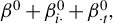
 has an additive structure:

where
$\beta _{i\cdot }^{0}$
 and
$\beta _{\cdot t}^{0}$
 are two
$K\times 1$
 random vectors. Without loss of generality, we impose the normalization condition that
$E(\beta _{i\cdot }^{0})=0$
 and leave
$E(\beta _{\cdot t}^{0}) $
 unrestricted.Footnote
1
$E(\beta _{\cdot t}^{0})$
 can be interpreted as the average effects of
$x_{it}$
 on
$y_{it}. \beta _{i\cdot }^{0}$
 and
$\beta _{\cdot t}^{0}$
 (or its centered version
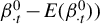
$\beta _{\cdot t}^{0}-E(\beta _{\cdot t}^{0}))$
 represent the effect heterogeneity along the individual and time dimensions, respectively. We allow
$\beta _{i\cdot }^{0}$
 and
$\beta _{\cdot t}^{0}$
 to be correlated with
$x_{it},$
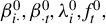
 therefore, model (1.1) is a correlated random-coefficient (CRC)-type model with IFEs. In this model, we treat
$\beta _{i\cdot }^{0}, \beta _{\cdot t}^{0}, \lambda _{i}^{0}, f_{t}^{0},$
 and
$R^{0}$
 all as unknown parameters. Note that we do not allow dynamic models in this article, that is,
$ x_{it}$
 cannot be the lagged dependent variable.Footnote
2
We propose a two-step estimation procedure for our model. In the first step, we obtain a preliminary consistent estimator of
$\beta _{i\cdot }^{0}, \beta _{\cdot t}^{0},$
 and
$\Theta ^{0}$
 via nuclear norm regularization (NNR), where
$\Theta ^{0}$
 is a
$T\times N$
 matrix with its
$\left (t,i\right ) $
 th element given by
$\lambda _{i}^{0\prime }f_{t}^{0}.$
 Nevertheless, due to the use of NNR, we can only establish slow convergence rates for these estimators. In particular, we can only establish the weak consistency of the NNR estimator of the low-rank matrix
$ \Theta ^{0}$
 in terms of Frobenius norm. But it is sufficient for us to obtain a consistent estimator of the number of factors, say, via a singular value thresholding procedure. In the second step, we adopt an iterative procedure to conduct post-NNR (PNNR) estimation of all parameters, including
$\beta _{i\cdot }^{0},\beta _{\cdot t}^{0},\lambda _{i}^{0}$
 , and
$f_{t}^{0}$
 . We establish the asymptotic properties of these estimators in the large panel framework where both N and T tend to infinity. One key challenge is to deal with the high dimensionality of the parameters. Note that the total dimension of
$\{\beta _{i\cdot }^{0},\beta _{\cdot t}^{0},\lambda _{i}^{0},f_{t}^{0}\}$
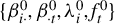 is
$ K\left (N+T-1\right ) +R^{0}\left (N+T\right ) ,$
 which increases with both N and
$T.$
 For example, in a reasonable setting where
$N=100, T=100, K=2,$
 and
$R^{0}=2,$
 it is close to 800.
As argued above, our model in (1.1) and (1.2) can be of independent interest and applied directly to many empirical studies where
$\{\beta _{i\cdot }^{0},\beta _{\cdot t}^{0}\}$
 are usually the parameters of interest. The model’s utility is further demonstrated by its application to estimating counterfactual outcomes, which is central to program evaluation and treatment effect analysis. Following Rubin’s potential outcome framework, let
$y_{it}^{1}$
 and
$y_{it}^{0}$
 be the potential treated (intervened) and untreated outcomes for individual i at time t, respectively. For example, consider the effect of economic liberalization (openness) on economic growth where the binary treatment indicator is whether a country is open and
$x_{it}$
 is some observable covariates (e.g., investment share) that can explain economic growth.
$ y_{it}^{1}$
 is the economic growth of country i at year t if it is open at year t, and
$y_{it}^{0}$
 is its economic growth if it is closed. The treatment effect is simply
$y_{it}^{1}-y_{it}^{0}.$
 The fundamental issue here is that we only observe either
$y_{it}^{1}$
 or
$y_{it}^{0}$
 but never both. We consider the treatment effect on the treated, that is, those countries which switch from “closed” to “open” in certain years. For those treated, we directly observe
$y_{it}^{1},$
 but
$y_{it}^{0}$
 is unobservable and counterfactual, which has to be estimated. We provide a general approach to estimate the counterfactual outcome in this framework. Specifically, we assume that the untreated potential outcome
$y_{it}^{0}$
 follows models (1.1) and (1.2) by taking into account the unobserved heterogeneity over both the countries and the years. Using the data of the control individuals (those who are never treated), we estimate
$\beta _{\cdot t}^{0}$
 and
$f_{t}^{0}$
 . Then we estimate the individual-specific
$ \beta _{i\cdot }^{0}$
 and
$\lambda _{i}^{0}$
 for the treated individuals and estimate the counterfactual untreated outcome for them. For details, see our Algorithm 2 in Section 4. We derive the asymptotic properties of various treatment effects on the treated based on our estimated counterfactual outcomes. Our approach can be viewed as an alternative to the popular synthetic control method (SCM) to estimate counterfactual outcomes. Relative to SCM, our approach can potentially exploit more information on covariates (
$x_{it}$
 ) when model (1.1) is correctly specified. In addition, we allow
$\beta _{\cdot t}$
 to have a nonstationary distribution. The nonstationarity of
$\beta _{\cdot t}$
 can invalidate many existing inference procedures applied to SCM, such as Chernozhukov, Wüthrich, and Zhu (Reference Chernozhukov, Wüthrich and Zhu2021), Masini and Medeiros (Reference Masini and Medeiros2021), and Masini and Medeiros (Reference Masini and Medeiros2022). This is because
$\beta _{\cdot t}$
 typically enters the error term of the SCM model, so nonstationary coefficients directly induce nonstationarity in the error term. Consequently, this violates a fundamental stationarity assumption underlying those inference methods. For a detailed discussion and evidence on these points, please refer to the simulations in Section 5 of the main text and Section S.7 of the Supplementary Material.
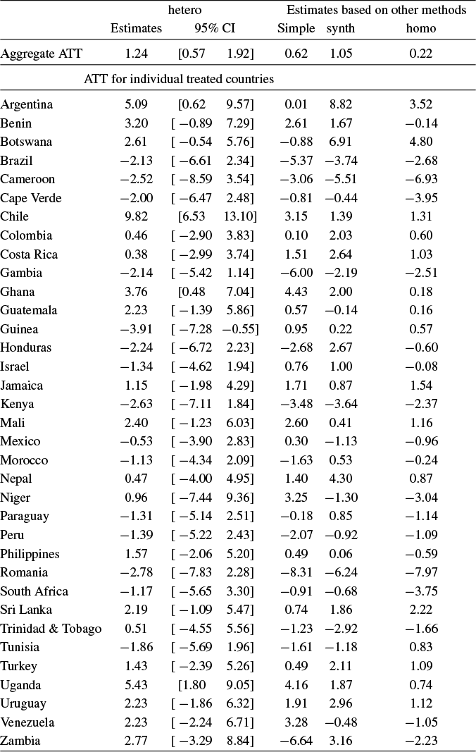
We apply our new method to evaluate the impact of economic liberalization on economic growth using panel data for 60 countries over 30 years (1965–1994). The outcome variable is annual economic growth, and the treatment indicator denotes whether a country is classified as “open.” Two key covariates—the investment share and consumption share of GDP—are included in the analysis. Our main finding is that liberalization exerts a positive and statistically significant effect: the aggregate average treatment effects on the treated (ATT) is 1.24% annual growth. Country-level ATT estimates reveal substantial heterogeneity: 20 countries exhibit positive effects, while 15 show negative effects. Additionally, we find that the investment share is positively associated with the untreated potential outcome, whereas the consumption share exerts a small negative effect. Overall, the results support the view that openness fosters economic growth, though the magnitude and direction of effects vary across countries.
Our article is closely related to several strands of literature. First, our article pertains to the large literature on panel data models (see, e.g., Hsiao, Reference Hsiao2022, for a review). Our model can be thought of as a generalization of many widely used panel data models. If we impose
$\beta _{i\cdot }^{0}+\beta _{\cdot t}^{0}$
 to be constant, our model becomes the standard panel data model with IFEs (see, e.g., Bai, Reference Bai2009; Moon and Weidner, Reference Moon and Weidner2015; Armstrong, Weidner, and Zeleneev, Reference Armstrong, Weidner and Zeleneev2026). If we restrict that
$\beta _{\cdot t}^{0}=0$
 and leave
$\beta _{i\cdot }^{0}$
 unrestricted, this is the random coefficient model (see, e.g., Pesaran, Reference Pesaran2006; Su, Shi, and Phillips, Reference Su, Shi and Phillips2016; Li, Cui, and Lu, Reference Li, Cui and Lu2020). If we impose that
$\beta _{i\cdot }^{0}=0$
 while leaving
$\beta _{\cdot t}^{0}$
 unrestricted, our model becomes the time-varying coefficient model (see, e.g., Zhu, Reference Zhu2017). If the factor structure
$ \lambda _{i}^{0\prime }f_{t}^{0}$
 is replaced by two-way additive fixed effects, our model reduces to the panel data model with two-dimensional heterogeneity studied in Keane and Neal (Reference Keane and Neal2020) and Lu and Su (Reference Lu and Su2023).
Second, our article is related to the literature on the estimation of counterfactual outcomes and treatment effects, which has been developing rapidly over the last two decades. Due to space limitations, here we only provide a brief review of the estimation methods with panel data. For cross-sectional data, see Imbens and Wooldridge (Reference Imbens and Wooldridge2009) for a review. In two seminal papers, Abadie and Gardeazabal (Reference Abadie and Gardeazabal2003) and Abadie, Diamond, and Hainmueller (Reference Abadie, Diamond and Hainmueller2010) propose the SCM to estimate counterfactual outcomes, which has been widely applied to many empirical contexts. SCM uses a weighted average of observed untreated outcomes of untreated individuals to estimate the counterfactual for those treated. As remarked in Athey and Imbens (Reference Athey and Imbens2017), SCM is arguably the most important development in program evaluation in the last decade. The literature on SCM has been developing rapidly in the last two decades (see Abadie, Reference Abadie2021, for an excellent review). We have seen extensive development on the generalization or inference on SCM in the last decade. For example, Doudchenko and Imbens (Reference Doudchenko and Imbens2016) generalize SCM by allowing the weights to be negative and their sum to differ from one, but with an elastic-net type penalty. Xu (Reference Xu2017) proposes a generalized SCM based on panels with IFEs where the slope coefficients of observable covariates are assumed to be homogeneous. Athey et al. (Reference Athey, Bayati, Doudchenko, Imbens and Khosravi2021) develop matrix completion estimators for counterfactuals. Arkhangelsky et al. (Reference Arkhangelsky, Athey, Hirshberg, Imbens and Wager2021) propose a synthetic difference-in-differences method. Li (Reference Li2020), Chernozhukov et al. (Reference Chernozhukov, Wüthrich and Zhu2021), Masini and Medeiros (Reference Masini and Medeiros2021), and Masini and Medeiros (Reference Masini and Medeiros2022) propose different inference methods for SCM, and Cattaneo, Feng, and Titiunik (Reference Cattaneo, Feng and Titiunik2021) develop prediction intervals for SCM. Typically, a certain form of stationarity of the error term is required for the validity of inferences considered in these papers and inferences can be invalid when nonstationarity is not properly accounted for, say when it appears in the parameter. More recently, Chen (Reference Chen2023) shows that SCM can be represented as an online learning algorithm and its predictions of counterfactual outcomes perform almost as well as an oracle weighted average of control units’ outcomes. Note that our estimator does not take a form of a weighted average of control units’ outcomes, thus it is not in the class of estimators considered in Chen (Reference Chen2023). In addition, we allow for nonstationarity in
$\left \{ \beta _{\cdot t}\right \} ,$
 in which case typical SCM inference procedures (e.g., Chernozhukov et al., Reference Chernozhukov, Wüthrich and Zhu2021) that fail to take into account the covariate part are asymptotically invalid.
Third, in terms of methodology, our approach is closely related to the burgeoning literature on the use of NNR in econometrics, statistics, and machine learning (see Koltchinskii, Lounici, and Tsybakov, Reference Koltchinskii, Lounici and Tsybakov2011; Negahban and Wainwright, Reference Negahban and Wainwright2011; Rohde and Tsybakov, Reference Rohde and Tsybakov2011; Negahban et al., Reference Negahban, Ravikumar, Wainwright and Yu2012; Bai and Ng, Reference Bai and Ng2019; Fan, Gong, and Zhu, Reference Fan, Gong and Zhu2019; Athey et al., Reference Athey, Bayati, Doudchenko, Imbens and Khosravi2021; Ma, Su, and Zhang, Reference Ma, Su and Zhang2022; Belloni et al., Reference Belloni, Chen, Padilla and Wang2023; Miao, Phillips, and Su, Reference Miao, Phillips and Su2023; Chernozhukov et al., Reference Chernozhukov, Hansen, Liao and Zhu2026; Moon and Weidner, Reference Moon and Weidner2026). All these previous works focus on the error bounds (in Frobenius norm) for the NNR estimators, except Ma et al. (Reference Ma, Su and Zhang2022), Miao et al. (Reference Miao, Phillips and Su2023), Moon and Weidner (Reference Moon and Weidner2026), and Chernozhukov et al. (Reference Chernozhukov, Hansen, Liao and Zhu2026), who study inference problems in linear/nonlinear panel or VAR models with low-rank structures. Like these latter authors, we simply use the NNR to obtain consistent initial estimators and our final objective is to establish the usual inference theory for the complete model in (1.1) and (1.2).
The rest of the article is structured as follows. In Section 2, we propose our estimation method for models (1.1) and (1.2). Section 3 establishes the asymptotic properties of the estimators. In Section 4, we show how to apply our model to estimate various treatment effects and study their asymptotic properties. Section 5 reports Monte Carlo simulation results. In Section 6, we apply our method to study the effect of economic liberalization on economic growth. Section 7 concludes. All proofs of the main results are relegated to the Appendix. The Supplementary Material includes some detailed analyses and additional simulation and empirical results.
Notation. Let
$\mathbb {I}_{m}$
 denote an
$m\times m$
 identity matrix. For a real
$m\times n$
 matrix
$A=(a_{ij})$
 , we use
$ \left \Vert A\right \Vert , \left \Vert A\right \Vert _{\text {sp}}$
 , and
$ ||A||_{\ast }$
 to denote its Frobenius norm, spectral norm, and nuclear norm, respectively:
$||A||_{\text {sp}}\equiv \mu _{1}(A)$
 ,
$||A||\equiv (\sum _{i=1}^{m}\sum _{j=1}^{n}a_{ij}^{2})^{1/2},$
 and
$||A||_{\ast }\equiv \sum _{k=1}^{m\wedge n}\mu _{k}(A),$
 where
$\mu _{k}(A)$
 denotes the kth largest singular value of A for
$k\leq m\wedge n\equiv \min (m,n)$
 and
$ \equiv $
 signifies a definitional relationship. Let
$\left \Vert A\right \Vert _{\infty }$
 and
$\left \Vert A\right \Vert _{1}$
 denote the
$L_\infty $
 and
$ L_1$
 norm of matrix A. That is,
$\left \Vert A\right \Vert _{\infty }$
 and
$ \left \Vert A\right \Vert _{1}$
 are the maximum absolute row sum and column sum of A. Let
$\mu _{\min }(A)\equiv \mu _{m\wedge n}(A)$
 and
$\mu _{\max }(A)\equiv \mu _{1}(A)$
 . Let
$A^{\prime }$
 denote the transpose of A. When A has full rank, let
${\mathbb {P}_{A}=A(A^{\prime }A)^{-1}A^{\prime }}$
 and
$ \mathbb {M}_{A}=\mathbb {I}_{m}-\mathbb {P}_{A}.$
 For a positive integer
$n,$
 let
$\left [ n\right ] \equiv \left \{ 1,2,\ldots ,n\right \} $
 . Let
$\mathrm {vec} (\cdot )$
 denote the usual vectorization operator. Let
$\mathrm {mat}(\cdot )$
 be the reverse operator of
$\mathrm {vec}$
 (
$\cdot $
 ):
$\mathrm {mat}(\mathrm {vec} (A))=A$
 . Let
$\otimes $
 denote the Kronecker product. Let
$\mathbf {1}\{\cdot \}$
 be the indicator function. Let
${\mathrm {blkdiag}}(A_1, \ldots , A_k) $
 represent a block-diagonal matrix with square diagonal blocks
$A_1, \ldots , A_k $
 . The symbol
$\overset {p}{\rightarrow }$
 denotes convergence in probability,
$ \overset {d}{\rightarrow }$
 convergence in distribution, and plim probability limit. We use
$\left (N,T\right ) \rightarrow \infty $
 to signify that N and T pass to infinity jointly.
2 THE MODEL AND ESTIMATION METHOD
In this section, we first introduce the panel data model with two-dimensional unobserved slope heterogeneity and IFEs. Then we propose a two-step approach to estimate the parameters in the model.
2.1 The Model
The scalar form of our model is given by

where
$x_{it}$
 ,
$f_{t}^{0}$
 ,
$\lambda _{i}^{0}$
 , and
$u_{it}$
 are defined as above. Note that
$\beta _{i\cdot }^{0}$
 and
$\beta _{\cdot t}^{0}$
 are not separately identified. In other words, equation (2.1) cannot be directly employed to construct a least-squares estimator. To achieve identification, we assume
$E(\beta _{i\cdot }^{0})=0$
 and leave
$ E(\beta _{\cdot t}^{0})$
 unrestricted. Define
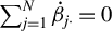
$\dot {\beta }_{i\cdot }=\beta _{i\cdot }^{0}-\frac {1}{N}\sum _{j=1}^{N}\beta _{j\cdot }^{0}$
 and
$\dot {\beta }_{\cdot t}=\beta _{\cdot t}^{0}+\frac {1}{N}\sum _{j=1}^{N}\beta _{j\cdot }^{0}$
 . By construction,
$\sum _{j=1}^{N}\dot {\beta }_{j\cdot }=0$
 . We can then rewrite the model as


Let
$\dot {B}^{(1)}\equiv \lbrack \dot {\beta }_{1\cdot }^{\prime },\ldots , \dot {\beta }_{N-1\cdot }^{\prime }]^{\prime }\in \mathbb {R}^{(N-1)K}$
 and
$ \dot {B}^{(2)}\equiv \lbrack \dot {\beta }_{\cdot 1}^{\prime },\ldots ,\dot { \beta }_{\cdot T}^{\prime }]^{\prime }\in \mathbb {R}^{TK}$
 . Equations (2.2) and (2.3) can be employed to construct a least squares estimator.
We establish two alternative representations of models (2.2) and (2.3). The vector representation facilitates the analysis of the least-squares estimators for elements in
$\dot {B}\equiv \lbrack \dot {B} ^{(1)\prime },\dot {B}^{(2)\prime }]^{\prime }$
 in the following discussion, while the matrix representation is particularly useful for studying the estimator associated with the factor structure.
To proceed, we introduce some notation. Let
$\mathbf {y}_{i\cdot }\equiv \lbrack y_{i1},y_{i2},\ldots ,y_{iT}]^{\prime } \in \mathbb {R}^{T}$
 ,
$ \mathbf {y}_{\cdot t}\equiv \lbrack y_{1t},y_{2t},\ldots ,y_{Nt}]^{\prime } \in \mathbb {R}^{N}$
 , and
$Y\equiv \lbrack \mathbf {y}_{1\cdot }^{\prime }, \mathbf {y}_{2\cdot }^{\prime },\ldots ,\mathbf {y}_{N\cdot }^{\prime }]^{\prime }\in \mathbb {R}^{NT}$
 . Define
$\mathbf {u}_{i\cdot },\mathbf {u} _{\cdot t},$
 and U analogously. Let
$\mathbf {x}_{i\cdot }\equiv \lbrack x_{i1},x_{i2},\ldots ,x_{iT}]^{\prime }\in \mathbb {R}^{T\times K}$
 and
$ \mathbf {x}_{\cdot t}\equiv \lbrack x_{1t},x_{2t},\ldots ,x_{Nt}]^{\prime }\in \mathbb {R}^{N\times K}$
 be the covariate matrices that may appear in equations for individual i and time t, respectively. Define

Let
$X^{(1,2)}\equiv \lbrack X^{(1)},X^{(2)}]$
 . Given the above notations, the model in (2.2) and (2.3) can be rewritten in an
$NT$
 -vector form:

where
$\theta ^{0}\equiv $
 vec
$(\Theta ^{0})$
 . The vector
$\dot { B}$
 stacks all free unit- and time-specific slope coefficients into a single
$(N+T-1)K\times 1$
 vector. Accordingly, for each pair
$(i,t)$
 , the corresponding row of
$X^{(1,2)}$
 consists of an expanded regressor vector, constructed by interacting
$x_{it}$
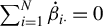
 with the full set of unit and time dummies, while imposing the normalization constraint
$\sum _{i=1}^{N}\dot { \beta }_{i\cdot }=0$
 . Consequently, the product
$X^{(1,2)}\dot {B}$
 is equivalent to a regression specification that includes all unit–time interactive effects involving
$x_{it}$
 . Next, we introduce the matrix representation. Denote the kth entries of
$x_{it}, \dot {\beta }_{i\cdot }$
 , and
$\dot {\beta }_{\cdot t}$
 as
$x_{k,it}$
 ,
$\dot {\beta }_{k,i\cdot }$
 , and
$ \dot {\beta }_{k,\cdot t},$
 respectively. Let
$\mathbf {X}_{k}$
 be a
$T\times N$
 matrix with
$(t,i)$
 th entry
$x_{k,it}$
 , for
$k\in \lbrack K]$
 . Similarly, we define
$\mathbf {Y}$
 and
$\mathbf {U}$
 . Then we have the matrix representation:

where
$\dot {\mathbf {B}}_{k,T}\equiv \mathrm {diag}(\dot {\beta }_{k,\cdot 1},\dot { \beta }_{k,\cdot 2},\ldots ,\dot {\beta }_{k,\cdot T})$
 and
$\dot {\mathbf {B}} _{k,N}\equiv \mathrm {diag}(\dot {\beta }_{k,1\cdot },\dot {\beta }_{k,2\cdot },\ldots ,\dot {\beta }_{k,N-1\cdot },-\sum _{i=1}^{N-1}\dot {\beta }_{k,i\cdot }) $
 are
$T\times T$
 and
$N\times N$
 diagonal matrices, respectively.
We now outline the main steps for estimating model (2.1):
-
1. Solve the nuclear-norm-regularized problem defined in (2.7) below. This step yields a consistent estimator of the matrix $\Theta ^{0}$
 in terms of Frobenius norm.
-
2. Determine the number of factors using (2.8) or other methods discussed below and obtain the initial estimators of the factors and factor loadings as in (2.9). This step provides consistent estimators of the number of factors, factors, and loadings.
-
3. Apply Algorithm 1, introduced in Section 2.3, to obtain the final estimators of the slope coefficients and latent factors and loadings. This step refines the estimators through iterations and produces the final estimators used for statistical inference.

2.2 Initial Estimation: Nuclear Norm Regularized Estimation
In this section, we produce initial estimators of the parameters in the model. Define the objective function as

where
$B\in \mathbb {R}^{(N-1+T)K}$
 ,
$\theta \equiv $
 vec
$(\Theta )$
 ,
$\Theta \in \mathbb {R}^{T\times N}$
 , and
$\gamma _{NT}$
 is a regularization parameter such that
$\gamma _{NT}\rightarrow 0$
 as
$\left (N,T\right ) \rightarrow \infty $
 . Then the initial estimator is given by

At any fixed
$\Theta $
 , minimizing
$\mathcal {L}_{NT}(B,\Theta )$
 is a least-squares problem. Formally, we can write

where
$\mathbb {M}_{x}\equiv \mathbb {M}_{X^{(1,2)}}$
 is the
$NT\times NT$
 projection matrix that projects out the columns of
$X^{(1,2)}.$
 Hence, minimizing
$\mathcal {L}_{NT}(B,\Theta )$
 can be achieved by minimizing
$ \mathcal {\tilde {L}}_{NT}(\Theta )+\gamma _{NT}\frac {\left \vert \left \vert \Theta \right \vert \right \vert _{\text {*}}}{\sqrt {NT}}.$
 That is,

Given the initial estimators
$\hat {B}_{o}$
 and
$\hat {\Theta } _{o} $
 , one can use various methods to determine the number of factors
$ R^{0}.$
 For example, we can estimate
$R^{0}$
 via the singular value thresholding as follows:

where
$\mu _{i}(\hat {\Theta }_{o})$
 denotes the ith largest singular value of
$\hat {\Theta }_{o}.$
 Alternatively, we can estimate
$R^{0}$
 by some other methods, including the information criteria and panel criteria methods of Bai and Ng (Reference Bai and Ng2002), the edge distribution estimator of Onatski (Reference Onatski2010), the eigenvalue ratio and growth ratio method of Ahn and Horenstein (Reference Ahn and Horenstein2013), and the cross-validation method of Jin, Miao, and Su (Reference Jin, Miao and Su2021).
Given
$\hat {R}$
 , we can obtain preliminary estimators of the factors and factor loadings. Consider the singular value decomposition (SVD) of
$\hat {\Theta }_{o}: \hat {\Theta }_{o}=\hat {L}\hat {D}\hat {V}^{\prime },$
 where
$\hat {D}=$
 diag
$(\mu _{1}(\hat {\Theta }_{o}),\ldots ,\mu _{N\wedge T}(\hat { \Theta }_{o})),$
 and
$\hat {L}$
 and
$\hat {V}$
 stack the left and right singular vectors of
$\hat {\Theta }_{o}$
 , respectively. We estimate
$F^{0}$
 and
$\Lambda ^{0}$
 , respectively, by

where
$\hat {L}_{\ast ,[\hat {R}]}$
 denotes a submatrix of
$\hat {L}$
 that contains its first
$\hat {R}$
 columns and
$\hat {D}_{[\hat {R}],[\hat {R} ]}\equiv $
 diag
$(\mu _{1}(\hat {\Theta }_{o}),\dots , \mu _{\hat {R}}(\hat {\Theta } _{o})).$

Remark 2.1. Here, we assume that
$\beta _{it}^{0}$
 follows an additive structure as in (1.2). Let
$\beta _{k,it}^{0}$
 ,
$\beta _{k,i\cdot }^{0}$
 , and
$\beta _{k,\cdot t}^{0}$
 denote the k-th elements of
$\beta _{it}^{0}$
 ,
$\beta _{i\cdot }^{0}$
 , and
$\beta _{\cdot t}^{0}$
 , respectively. Since
$\beta _{k,it}^{0}=(\beta _{k,i\cdot }^{0},1)(1,\beta _{k,\cdot t}^{0})^{\prime }$
 , the
$N\times T$
 matrix
$\boldsymbol {\beta } _{k}^{0}\equiv \{\beta _{k,it}^{0}:i\in \lbrack N],~t\in \lbrack T]\}$
 has rank two in general for each
$k\in \lbrack K]$
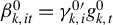
 . It is possible to generalize
$\beta _{k,it}^{0}$
 to have a generic low-rank (factor) structure of rank
$ R_{k}$
 , namely,
$\beta _{k,it}^{0}=\gamma _{k,i}^{0\prime }g_{k,t}^{0}$
 , where
$\gamma _{k,i}^{0}$
 and
$g_{k,t}^{0}$
 are
$R_{k}\times 1$
 vectors for
$ k\in \lbrack K]$
 . In that case, the NNR needs to be applied to the slope coefficients too, as in Chernozhukov et al. (Reference Chernozhukov, Hansen, Liao and Zhu2026). However, inference in such settings typically requires stronger assumptions and a sample-splitting procedure, which we do not pursue in this article. See Remarks 3.6 and 3.7 in Section 3.3 below.
Remark 2.2. While both our study and Moon and Weidner (Reference Moon and Weidner2026) utilize NNR, our contributions are distinct and address a fundamentally more challenging problem. Moon and Weidner (Reference Moon and Weidner2026) apply NNR to estimate a homogeneous model, where the slope coefficient
$ \beta _{it}^{0}$
 is assumed constant. In contrast, we consider a heterogeneous model, introducing high-dimensional parameters via the additive form
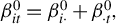
$\beta _{it}^{0}=\beta _{i\cdot }^{0}+\beta _{\cdot t}^{0},$
 varying across both individuals and time. This distinction is crucial. As noted in the literature (e.g., Jiang et al., Reference Jiang, Yang, Gao and Hsiao2021), the convergence of PCA estimators in panels with IFEs often hinges on a suitable initial estimator. The NNR method provides a consistent starting point that facilitates convergence. However, our article is one of the first to develop estimation and inference for a panel with two-dimensional slope heterogeneity and IFEs. Therefore, while NNR serves a similar initial-stage purpose, the subsequent analysis diverges completely.
2.3 Post Nuclear Norm Regularized Estimation
In this section we propose an iterative procedure to obtain updated estimators of the regression coefficients, the factors, and the factor loadings. The algorithm goes as follows:
Algorithm 1 Iterated estimator for
$\dot {B}$

-
1. For $s=0$
, set
$\hat {F}^{(s)}=\hat {F}_{o}$
and
$\hat {\Lambda }^{(s)}= \hat {\Lambda }_{o}.$
-
2. Update $\hat {B}_{s}$
by (2.10) $$ \begin{align} \hat{B}_{s}\equiv & \arg \min_{B}\min_{g\in \mathbb{R}^{T\times \hat{R} },h\in \mathbb{R}^{N\times \hat{R}}}\left\Vert \mathrm{mat}(Y-X^{(1,2)}B)- \hat{F}^{(s)}h^{\prime }-g\hat{\Lambda}^{(s)\prime }\right\Vert ^{2} \notag \\ =& \left[ X^{(1,2)\prime }(\mathbb{M}_{\hat{\Lambda}^{(s)}}\otimes \mathbb{M} _{\hat{F}^{(s)}})X^{(1,2)}\right] ^{-1}X^{(1,2)\prime }(\mathbb{M}_{\hat{ \Lambda}^{(s)}}\otimes \mathbb{M}_{\hat{F}^{(s)}})Y. \end{align} $$
The corresponding $s$
th step estimators for
$\dot {\beta }_{j\cdot }$
and
$ \dot {\beta }_{\cdot t}$
are denoted as
$\hat {\beta }_{j\cdot }^{(s)}$
and
$ \hat {\beta }_{\cdot t}^{(s)}$
, respectively. -
3. Update $\hat {F}^{(s+1)}$
and
$\hat {\Lambda }^{(s+1)} $
based on
$ \textrm {mat}[Y-X^{(1,2)}\hat {B}_{s}].$
Specifically, let SVD of
$\textrm {mat} [Y-X^{(1,2)}\hat {B}_{s}]$
be
$\mathrm {mat}[Y-X^{(1,2)}\hat {B}_{s}]=\hat {L} ^{(s+1)}\hat {D}^{(s+1)}\hat {V}^{^{(s+1)}\prime }.$
Estimate
$F^{0}$
and
$ \Lambda ^{0}$
, respectively, by $$ \begin{align*} \hat{F}^{(s+1)}=\sqrt{T}\hat{L}_{\ast ,[\hat{R}]}^{(s+1)}\text{ and }\hat{ \Lambda}^{(s+1)}=\hat{V}_{\ast ,[\hat{R}]}^{(s+1)}\hat{D}_{[\hat{R}],[\hat{R} ]}^{(s+1)}/\sqrt{T}, \end{align*} $$where $\hat {L}_{\ast ,[\hat {R}]}^{(s+1)}$
and
$\hat {V}_{\ast ,[\hat {R} ]}^{(s+1)}$
denote submatrices of
$\hat {L}^{(s+1)}$
and
$\hat {V}^{(s+1)}$
, respectively, consisting of their first
$\hat {R}$
columns.
-
4. Iterate steps 2 and 3 for, $s^{\ast }\geq 2$
times.Set $\hat {B}\equiv \hat {B}_{s^{\ast }}$
. Similar to the definitions
$\dot {B} =[\dot {\beta }_{1\cdot }^{\prime },\ldots ,\dot {\beta }_{N-1\cdot }^{\prime },\dot { \beta }_{\cdot 1}^{\prime } \ldots ,\dot {\beta }_{\cdot T}^{\prime }]^{\prime }$
, we set
$\hat {B}\equiv \lbrack \hat {\beta }_{1\cdot }^{\prime },\ldots ,\hat { \beta }_{N-1\cdot }^{\prime }, \hat {\beta }_{\cdot 1}^{\prime },\ldots ,\hat { \beta }_{\cdot T}^{\prime }]^{\prime }.$
The estimator for
$\dot {\beta } _{N\cdot }$
is given by
$\hat {\beta }_{N\cdot }=-\sum _{i=1}^{N-1}\hat {\beta } _{i\cdot }$
. Let
$\hat {F}=\hat {F}^{(s^{\ast })}$
and
$\hat {\Lambda }=\hat { \Lambda }^{(s^{\ast })}$
. Denote
$t$
th row of
$\hat {F}$
as
$\hat {f} _{t}^{\prime }$
and
$i$
th row of
$\hat {\Lambda }$
as
$\hat {\lambda } _{i}^{\prime }$
.













Note that the iterations in Algorithm 1 alternate between updating
$\hat {B} _{s}$
 and
$(\hat {F}^{(s)},\hat {\Lambda }^{(s)})$
 for each iteration index s. However, the algorithm does not require numerical convergence. Instead, it can be terminated after any finite number of iterations
$s^{\ast }\geq 2$
 . The advantages of this approach are twofold:
-
1. Theoretical Perspective: We do not require the solution to correspond to the global minimum of an optimization problem. As long as the initial estimators of the factors and factor loadings are consistent, we can show that a finite number of iterations yields the desired asymptotic properties. Moreover, our theoretical analysis indicates that stopping at $s^{\ast }=2$
is sufficient, as additional iterations do not improve the asymptotic efficiency of the estimators in theory. -
2. Practical Perspective: In implementation, it is unnecessary to verify numerical convergence, nor is there a concern that the algorithm may become trapped in a local minimum.

3 ASYMPTOTIC THEORY
In this section, we study asymptotic properties of the initial estimator, the infeasible estimator that assumes
$F^{0}$
 and
$\Lambda ^{0}$
 are observed as an intermediate step and the feasible estimator.
3.1 Asymptotic Properties of the Initial Estimators
To study the asymptotic properties of the initial estimators, we make the following assumptions.
Assumption 1. For
$\gamma _{NT}=C_{\gamma }(N^{-1/2}+T^{-1/2})$
 , where
$ C_{\gamma }$
 is a sufficiently large positive constant, we have
$ (NT)^{-1/2}||$
 mat
$(\mathbb {M}_{x}U)||_{sp}\leq \frac {\gamma _{NT}}{2}$
 with probability approaching one (w.p.a.1).
Assumption 2. (Restricted Strong Convexity)
Let
$\mathbb {C} _{NT}\equiv \{\Theta \in \mathbb {R}^{T\times N}:\left \Vert \mathbb {M} _{F^{0}}\Theta \mathbb {M}_{\Lambda ^{0}}\right \Vert _{\ast }\leq 3\left \Vert \Theta -\mathbb {M}_{F^{0}}\Theta \mathbb {M}_{\Lambda ^{0}}\right \Vert _{\ast }\}.$
 There exists a
$\mu>0,$
 independent of N and T, such that for any
$\theta \in \mathbb {R}^{NT}$
 with
$\mathrm {mat}(\theta )\in \mathbb {C}_{NT}$
 , we have
$\theta ^{\prime }\mathbb {M}_{x}\theta \geq \mu \theta ^{\prime }\theta $
 , w.p.a.1 conditional on
$(\Lambda ^{0},F^{0})$
 .
Assumption 1 imposes some regularity conditions on
$\mathbb {M} _{x}U.$
 It is close to the condition imposed on the tuning parameter in Lemma 2 of Moon and Weidner (Reference Moon and Weidner2026), which studies the model with homogeneous slope coefficients. As one can argue, it suffices to choose
$\gamma _{NT}=C_{\gamma }(N^{-1/2}+T^{-1/2})$
 for some sufficiently large positive constant
$C_{\gamma }$
 to ensure Assumption 1 to be satisfied under some primitive conditions on
$\{x_{it}, u_{it}\}$
 . Such a rate ensures that the NNR estimator of
$\Theta $
 exhibits the optimal rate of convergence in terms of Frobenius norm (see Theorem 3.1 below). In our simulations and application, we follow the lead of Miao et al. (Reference Miao, Phillips and Su2023) and set
$\gamma _{NT}=0.5\max (N^{-1/2},T^{-1/2})$
 for simplicity, and leave the optimal choice of
$\gamma _{NT}$
 for future research.
Assumption 2 imposes the celebrated restricted strong convexity (RSC) condition that was first introduced by Negahban and Wainwright (Reference Negahban and Wainwright2012) and Negahban et al. (Reference Negahban, Ravikumar, Wainwright and Yu2012). We conjecture that this condition can be verified under more primitive assumptions by adapting the approach of Chernozhukov et al. (Reference Chernozhukov, Hansen, Liao and Zhu2026), accounting for the additional complexity introduced by the high-dimensional structure of our slope coefficients (see also Hong, Su, and Jiang, Reference Hong, Su and Jiang2023; Moon and Weidner, Reference Moon and Weidner2026).
The following theorem studies the consistency of the nuclear-norm regularized estimator
$\hat {\Theta }_{o}$
 in terms of the Frobenius norm.
Theorem 3.1. Suppose Assumptions 1 and 2 hold. We have that
$\Vert \hat {\Theta }_{o}-\Theta ^{0}\Vert /\sqrt {NT}\leq 3\sqrt { 2R^{0}}\gamma _{NT}/\mu $
 , w.p.a.1.
Theorem 3.1 indicates that we can estimate the large-dimensional matrix
$\Theta ^{0}$
 consistently in terms of the Frobenius norm. Note that
$ \Theta ^{0}$
 is a high-dimensional matrix with
$NT$
 entries and
$\Vert \Theta ^{0}\Vert =O_{P}(\sqrt {NT})$
 in general. This explains why we need to normalize
$\Vert \hat {\Theta }_{o}-\Theta ^{0}\Vert $
 by
$\sqrt {NT}$
 in Theorem 3.1.
Let
$\max _{i}=\max _{1\leq i\leq N}$
 and
$\max _{t}=\max _{1\leq t\leq T}$
 . Define
$\max _{i,j}$
 ,
$\max _{i,t}$
 ,
$\max _{t,s}$
 ,
$\min _{i}$
 , and
$\min _{t}$
 analogously. Next, we impose an assumption on the common factors and factor loadings.
Assumption 3. (Conditions on Factor Structure)
-
(i) $\left \Vert \frac {1}{N}\Lambda ^{0\prime }\Lambda ^{0}-\Sigma _{\Lambda }\right \Vert =O_{P}(N^{-1/2})$
for some
$\Sigma _{\Lambda }>0$
and
$\left \Vert \frac {1}{T} F^{0\prime }F^{0}-\Sigma _{F}\right \Vert =O_{P}(T^{-1/2})$
for some
$\Sigma _{F}>0.$
-
(ii) The eigenvalues of $\Sigma _{F}^{1/2}\Sigma _{\Lambda }\Sigma _{F}^{1/2} $
are all distinct. -
(iii) $\max _{i}||\lambda _{i}^{0}||=O_{P}(\log N)$
and
$ \max _{t}||f_{t}^{0}||=O_{P}(\log T)$
.




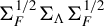


Assumption 3(i) and (ii) posits a strong factor structure, a standard condition widely adopted in the literature (see, e.g., Bai and Ng, Reference Bai and Ng2002; Bai, Reference Bai2003, Reference Bai2009; Su et al., Reference Su, Shi and Phillips2016; Moon and Weidner, Reference Moon and Weidner2017; Miao et al., Reference Miao, Phillips and Su2023, among others). Armstrong et al. (Reference Armstrong, Weidner and Zeleneev2026) propose a robust method for the estimation and inference of the slope coefficients in homogeneous panels involving weak factors. Assumption 3(iii) further imposes a uniform bound on the latent factors and factor loadings, which serves to facilitate the theoretical analysis in the subsequent sections. It holds when both
$\lambda _{i}^{0}$
 and
$f_{t}^{0}$
 are sub-exponentially distributed.
The following theorem reports the consistency of
$\hat {R}, \hat {F}_{o},$
 and
$\hat {\Lambda }_{o}.$

Theorem 3.2. Suppose Assumptions 1–3 hold. Then we have
(i)
$P(\hat {R}=R^{0})\rightarrow 1$
 as
$\left (N,T\right ) \rightarrow \infty $
 .
(ii)
$\frac {1}{\sqrt {T}}\left \Vert \hat {F}_{o}-F^{0}\tilde {H}\right \Vert =O_{P}\left (\gamma _{NT}\right ) $
 and
$\Vert \mathbb {M}_{\hat {F}_{o}}- \mathbb {M}_{F^{0}}\Vert _{sp}=O_{P}\left (\gamma _{NT}\right ) $
 , where
$ \tilde {H}$
 is an asymptotically nonsingular rotation matrix defined in the proof.
(iii)
$\frac {1}{\sqrt {N}}\left \Vert \hat {\Lambda }_{o}-\Lambda ^{0}(\tilde {H} ^{-1})^{\prime }\right \Vert =O_{P}\left (\gamma _{NT}\right ) $
 and
$\Vert \mathbb {M}_{\hat {\Lambda }_{o}}-\mathbb {M}_{\Lambda ^{0}}\Vert _{sp}=O_{P}\left (\gamma _{NT}\right ) $
 .
Theorem 3.2(i) indicates that
$\hat {R}$
 is a consistent estimator of
$R^{0}.$
 Theorem 3.2(ii) indicates that the columns of
$\hat {F}_{o}$
 and
$F^{0}$
 span the same space asymptotically, so do the columns of
$\hat {\Lambda }_{o}$
 and
$\Lambda ^{0}.$

Remark 3.1. The result in Theorem 3.1 bears a conceptual resemblance to Lemma 2 of Moon and Weidner (Reference Moon and Weidner2026), despite the significant increase in the number of regressors due to our two-dimensional heterogeneity. Theorem 3.2 follows from Theorem 3.1 under standard conditions on the factors and loadings in Assumption 3—a result also attainable for the homogeneous panel. The key mechanism that accommodates the high dimensionality of our slope parameters
$\left \{ \beta _{i\cdot }^{0}\right \} $
 and
$\left \{ \beta _{\cdot t}^{0}\right \} $
 is the high-level RSC condition in Assumption 2. It could be substantially more challenging to verify this RSC condition for our heterogeneous model than for a homogeneous one, which is the necessary statistical price for our more flexible specification.
Remark 3.2. Crucially, the results in Theorems 3.1 and 3.2 are preliminary. Despite the fact that we can establish the consistency of
$\hat {\Theta }_{o}, \hat {F}_{o},$
 and
$\hat {\Lambda }_{o}$
 in terms of the Frobenius norm, we cannot obtain pointwise consistency or asymptotic distributions for the elements of these estimators. The primary role of Theorems 3.1 and 3.2 is to facilitate the analysis of the subsequent iterative (post-NNR) estimators. It is in the study of these post-NNR estimators where the substantive theoretical challenges and novelties of our article emerge. Due to the high-dimensional nature of the slope parameters, analyzing the asymptotic properties of the estimators for
$\beta _{i\cdot }^{0}$
 and
$\beta _{\cdot t}^{0}$
 becomes highly complex. As indicated in Section S.1 of the Supplementary Material, even the analysis of the infeasible estimators (assuming observed factors and loadings) is nontrivial. Furthermore, as detailed in Section S.2 of the Supplementary Material, the unobserved nature of the factors and loadings introduces additional layers of complication, substantially deepening the theoretical analysis beyond the homogeneous case.
3.2 Asymptotic Properties of the Infeasible Estimator
Despite the consistency of the initial estimators
$\hat {F}^{(0)}$
 and
$\hat { \Lambda }^{(0)},$
 it is challenging to study the asymptotic properties of
$ \hat {\beta }_{i\cdot }$
 and
$\hat {\beta }_{\cdot t}$
 directly. Below we first study the asymptotic properties of their infeasible version as given in (3.1) and then study those of the feasible one. Our results show that the difference between the feasible and infeasible versions is asymptotically negligible. As an intermediate result, we first study the infeasible estimator in (3.1) in this section. Now we formally introduce the infeasible estimator. Given
$F^{0}$
 and
$\Lambda ^{0}$
 are observed, we can estimate
$\dot {B}$
 by

Similar to the definition
$\dot {B}=[\dot {\beta }_{1\cdot }^{\prime },\ldots ,\dot { \beta }_{N-1\cdot }^{\prime },\dot {\beta }_{\cdot 1}^{\prime }, \ldots ,\dot { \beta }_{\cdot T}^{\prime }]^{\prime }$
 , we set
$\check {B}\equiv \lbrack \check {\beta }_{1\cdot }^{\prime }, \ldots ,\check {\beta }_{N-1\cdot }^{\prime }, \check {\beta }_{\cdot 1}^{\prime },\ldots ,\check {\beta }_{\cdot T}^{\prime }]^{\prime }$
 . The infeasible estimator for
$\dot {\beta }_{N\cdot }$
 is given by
$\check {\beta }_{N\cdot }=-\sum _{i=1}^{N-1}\check {\beta }_{i\cdot }$
 . In Section S.1 of the Supplementary Material, we show that
$X^{(1,2)\prime }(\mathbb {M}_{\Lambda ^{0}}\otimes \mathbb {M}_{F^{0}})X^{(1,2)}$
 is invertible asymptotically. Therefore,
$\check {B}$
 is well defined in large samples.
Remark 3.3. The infeasible estimator in equation (3.1) can be applied to estimate a heterogeneous panel data model that includes both observed time-invariant regressors
$\lambda _{i}^{0}$
 and factors
$f_{t}^{0}$
 :

where
$g_{t}$
 and
$\gamma _{i}$
 are unknown coefficients.Footnote
3
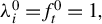
In particular, the heterogeneous panel data model with two-way fixed effects (TWFE) model, as in Lu and Su (Reference Lu and Su2023), arises as a special case. When
$\lambda _{i}^{0}=f_{t}^{0}=1,$
 the IFE structure simplifies to
$\lambda _{i}^{0\prime }g_{t}+\gamma _{i}^{\prime }f_{t}^{0}=g_{t}+\gamma _{i}$
 , which represents the standard TWFE specification. An important distinction lies in the assumptions regarding the regressors
$x_{it}.$
 Lu and Su (Reference Lu and Su2023) impose the condition that
$x_{it}$
 ’s behave as idiosyncratic errors after projecting out the individual and time effects. Our assumptions on
$x_{it}$
 are more general and less restrictive. Consequently, the theoretical results developed in this section also apply directly to inference on the slope coefficients
$ \beta _{i\cdot }^{0}$
 and
$\beta _{\cdot t}^{0}$
 within the specification described above.
To study the asymptotic properties of the infeasible estimator, we first introduce some notation and impose two regularity assumptions. Let
$\dot { \mathbf {x}}_{i\cdot }\equiv \mathbb {M}_{F^{0}}\mathbf {x}_{i\cdot }$
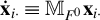 , and let
$\dot {x}_{it}$
 denote the transpose of the t’th row of
$\dot {\mathbf {x}} _{i\cdot }$
 . Similarly, define
$\ddot {\mathbf {x}}_{\cdot t}\equiv \mathbb {M} _{\Lambda ^{0}}\mathbf {x}_{\cdot t}$
 and
$\ddot {x}_{it}$
 . Define

Let
$\mathbf {Q}_{12}$
 be an
$(N-1)\times T$
 block-partitioned matrix whose
$ (i,t)$
 -th block (of size
$K\times K$
 ) is given by
$\dot {x}_{it}\ddot {x} _{it}^{\prime }-\frac {1}{N-1}\sum _{j=1}^{N-1}\dot {x}_{jt}\ddot {x} _{jt}^{\prime },\text { for }i\in \lbrack N-1], t\in \lbrack T].$
 Let
$ \delta _{NT}=\min (\sqrt {N},\sqrt {T})$
 .
Assumption 4. (Conditions on Regressors)
For some universal positive constants
$0<c_{1}<c_{2}<\infty $
 , we have
(i)
$\min _{i}\mu _{\min }(\dot {\mathbf {s}}_{i\cdot })\geq c_{1}$
 ,
$ \min _{t}\mu _{\min }(\ddot {\mathbf {s}}_{\cdot t})\geq c_{1}$
 ,
$\max _{i}\mu _{\max }(\dot {\mathbf {s}}_{i\cdot })\leq c_{2}$
 , and
$\max _{t}\mu _{\max }(\ddot {\mathbf {s}}_{\cdot t})\leq c_{2}$
 w.p.a.1;
(ii)
$\max _{i}T^{-1}\sum _{t=1}^{T}\left \Vert x_{it}\right \Vert ^{\ell }=O_{P}(1)$
 ,
$\max _{t}N^{-1}\sum _{i=1}^{N}\left \Vert x_{it}\right \Vert ^{\ell } =O_{P}(1)$
 for some
$\ell>4$
 ,
$\max _{i,t}\left \Vert x_{it}\right \Vert =O_{P}[\log (NT)], \max _{i}\left \Vert x_{it}\right \Vert =O_{P}[\log (N)],$
 and
$\max _{t}\left \Vert x_{it}\right \Vert =O_{P}[\log (T)];$

(iii) there exists a sequence
$\alpha _{NT}\rightarrow 0$
 .
$||\mathbf {Q} _{12}||_{\text {sp}}/\sqrt {NT}=O_{P}(\alpha _{NT}), ||\mathbb {M}_{F^{0}} \mathbf {X}_{k}||_{\text {sp}}/ \sqrt {NT}=O_{P}(\alpha _{NT})$
 and
$||\mathbf {X} _{k}\mathbb {M}_{\Lambda ^{0}}|||_{\text {sp}}/\sqrt {NT}=O_{P}(\alpha _{NT})$
 for all
$k\in \left [ K\right ] $
 .
Assumption 4 imposes regularity conditions on
$\dot {\mathbf {s}} _{i\cdot }$
 ,
$\ddot {\mathbf {s}}_{\cdot t}$
 ,
$x_{it}$
 ,
$f_{t}^{0}$
 , and
$ \lambda _{i}^{0}$
 . Assumption 4(i) introduces specific regularity requirements on
$\dot {\mathbf {s}}_{i\cdot }$
 and
$\ddot {\mathbf {s}}_{\cdot t} $
 , which are constructed from the de-factored and de-factor-loading versions of
$x_{it}$
 , denoted by
$\dot {x}_{it}$
 and
$\ddot {x}_{it}$
 , respectively. These conditions can be verified under suitable primitive assumptions, although they do exclude certain cases. Assumption 4 (ii) holds under mild moment and weak dependence conditions on the sequence
$ \{x_{it}\}$
 . Assumption 4(iii) is central for ensuring the asymptotic non-singularity of the Gram matrix
$X^{(1,2)\prime }(\mathbb {M} _{\Lambda }\otimes \mathbb {M}_{F})X^{(1,2)}$
 . For discussions on low-rank covariates, see, for example, Moon and Weidner (Reference Moon and Weidner2017) and Moon and Weidner (Reference Moon and Weidner2026).
Remark 3.4. Assumption 4(iii) eliminates the possibility of low-rank regressors in
$x_{it}$
 as in Bai (Reference Bai2009) and Armstrong et al. (Reference Armstrong, Weidner and Zeleneev2026). In particular, rank-one regressors, including
$x_{it}$
 that vary only across i or only across t will certainly lead to an identification issue. We present a simple example here. Consider the model in Remark 3.3. Suppose a scalar
$x_{it}$
 has rank one. Then it can be expressed as
$x_{it}=a_{i}e_{t}$
 , where
$a_{i}$
 and
$e_{t}$
 are both scalars that take value 0 with zero probability. For this case, the model specification suffers from a fundamental identification problem. For any vectors
$\delta _{1}$
 and
$\delta _{2}$
 of conformable dimensions, we have

and similarly,

where
$\dot {\beta }_{\cdot t}^{\ast }\equiv \dot {\beta }_{\cdot t}+\frac { \delta _{1}^{\prime }f_{t}^{0}}{e_{t}}, \gamma _{i}^{\ast }\equiv \gamma _{i}-a_{i}\delta _{1}, \dot {\beta }_{i\cdot }^{\ast }\equiv \dot {\beta } _{i\cdot }+\frac {\delta _{2}^{\prime }\lambda _{i}^{0}}{a_{i}},\quad $
 and
$ g_{t}^{\ast }\equiv g_{t}-e_{t}\delta _{2}.$
 This algebraic equivalence demonstrates that the parameters in the model described in Remark 3.3 are not identified in the presence of rank-one regressors. This issue directly results in singular Gram matrix
$X^{(1,2)\prime }(\mathbb {M} _{\Lambda ^{0}}\otimes \mathbb {M}_{F^{0}})X^{(1,2)}$
 . Further details are provided in Section S.6 of the Supplementary Material.
Assumption 5. (Conditions on Error Terms)
-
(i) $\max _{t}\left \Vert \mathbf {u}_{\cdot t}\right \Vert =O_{P}(\sqrt {N}), \max _{i}\left \Vert \mathbf {u}_{i\cdot }\right \Vert =O_{P}(\sqrt {T}), ||\mathbf {U}||_{\text {sp} }=O_{P}(\sqrt {N+T})$
,
$||\mathbf {U}^{\prime }\mathbf {U}||_{sp}=O_{P}(T)$
and
$||\mathbf {U}\mathbf {U}^{\prime }||_{sp}=O_{P}(N);$
-
(ii) $||\sum _{i=1}^{N}\sum _{t=1}^{T}\lambda _{i}^{0}f_{t}^{0\prime }u_{it}||=O_{P}(\sqrt {NT})$
,
$\sum _{t=1}^{T}x_{it}u_{it}=O_{P}(\sqrt {T})$
,
$ \sum _{i=1}^{N}x_{it}u_{it}=O_{P}(\sqrt {N})$
,
$\sum _{t=1}^{T}f_{t}^{0}u_{it}$
$=O_{P}(\sqrt {T})$
, and
$\sum _{i=1}^{N}\lambda _{i}^{0}u_{it}=O_{P}(\sqrt {N} ) $
; -
(iii) $\sum _{i=1}^{N}||\sum _{t=1}^{T}x_{it}u_{it}||^{2}=O_{P}(NT)$
and
$ \sum _{t=1}^{T}||\sum _{i=1}^{N}x_{it}u_{it}||^{2}=O_{P}(NT);$
-
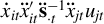
(iv) $\sum _{i=1}^{N-1}\sum _{t=1}^{T}\dot {\mathbf {s}}_{i\cdot }^{-1}\dot {x} _{it}u_{it}=O_{P}(\sqrt {NT})$
and
$\sum _{i=1}^{N}\sum _{t=1}^{T}\dot {\mathbf {s }}_{i\cdot }^{-1}\dot {x}_{it}u_{it}=O_{P}(\sqrt {NT})$
; -
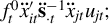
(v) $\max _{i}\left \Vert \sum _{t=1}^{T}\sum _{j=1}^{N}\varepsilon _{i,jt}\right \Vert =O_{P}(\sqrt {NT}\log N)$
for
$\varepsilon _{i,jt}=\lambda _{j}^{0}u_{jt}u_{it},x_{it}\lambda _{j}^{0\prime }u_{jt}$
,
$\dot {x}_{it} \ddot {x}_{it}^{\prime }\ddot {\mathbf {s}}_{\cdot t}^{-1}\ddot {x}_{jt}u_{jt}$
, and
$\ f_{t}^{0}\ddot {x}_{it}^{\prime }\ddot {\mathbf {s}}_{\cdot t}^{-1}\ddot { x}_{jt}u_{jt};$
-
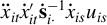
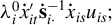
(vi) $\max _{t}\left \Vert \sum _{s=1}^{T}\sum _{i=1}^{N}\varepsilon _{is,t}\right \Vert =O_{P}(\sqrt {NT}\log T)$
for
$\varepsilon _{is,t}=f_{t}^{0}u_{is}u_{it},x_{is}f_{s}^{0\prime }u_{is}$
,
$\ddot {x}_{it} \dot {x}_{it}^{\prime }\dot {\mathbf {s}}_{i\cdot }^{-1}\dot {x}_{is}u_{is}$
, and
$\lambda _{i}^{0}\dot {x}_{it}^{\prime }\dot {\mathbf {s}}_{i\cdot }^{-1} \dot {x}_{is}u_{is};$
-
(vii) $\max _{i}\left \Vert \sum _{t=1}^{T}\varepsilon _{it}\right \Vert =O_{P}(\sqrt {T}\log N)$
for
$\varepsilon _{it}=x_{it}u_{it}$
and
$f_{t}^{0}u_{it}$
, and
$\max _{t}\left \Vert \sum _{i=1}^{N}\varepsilon _{it}\right \Vert = O_{P}(\sqrt {N}\log T)$
for
$\varepsilon _{it}=x_{it}u_{it}$
and
$\lambda _{i}^{0}u_{it}$
.























Assumption 5 imposes some high-level conditions on terms related to
$u_{it}$
 ’s. Assumption 5(i) is standard in the literature on factor models (see, e.g., Lu and Su, Reference Lu and Su2016; Moon and Weidner, Reference Moon and Weidner2017, Reference Moon and Weidner2026; Su and Wang, Reference Su and Wang2017; Chernozhukov et al., Reference Chernozhukov, Hansen, Liao and Zhu2026). Moon and Weidner (Reference Moon and Weidner2017) provide several examples to verify it. The rate conditions in Assumption 5(ii)–(vii) can be verified under some primitive conditions on
$\left \{ x_{it},\text { } f_{t}^{0},\text { }u_{it}\right \} $
 by calling up certain exponential inequalities. Assumption 5(ii) imposes pointwise asymptotic rate conditions on the relevant partial sums. In particular,
$ \sum _{t=1}^{T}x_{it}u_{it}=O_{P}(\sqrt {T})$
 is interpreted for each fixed i, and
$\sum _{i=1}^{N}x_{it}u_{it}=O_{P}(\sqrt {N})$
 is interpreted for each fixed t; neither condition is intended to hold uniformly over its free index. The aggregate rate conditions required in our analysis are imposed separately in Assumption 5(iii) and (iv), whereas Assumption 5(v)–(vii) provides the required uniform bounds through maxima over the relevant indices.
The following theorem establishes the asymptotic linear expansions of
$ \check {\beta }_{i\cdot }$
 and
$\check {\beta }_{\cdot t}.$

Theorem 3.3. Suppose that
$N^{-1/2}\log ^{2}T+T^{-1/2}\log ^{2}N\rightarrow 0$
 as
$(N,T)\rightarrow \infty $
 , and Assumptions 3–5 hold. Then we have
(i)
$\check {\beta }_{i\cdot }-\dot {\beta }_{i\cdot }=(\mathbf {x}_{i\cdot }^{\prime }\mathbb {M}_{F^{0}}\mathbf {x}_{i\cdot })^{-1}\mathbf {x}_{i\cdot }^{\prime }\mathbb {M}_{F^{0}}\mathbf {u}_{i\cdot }+o_{P}(1/\sqrt {T})$
 uniformly over
$i\in \left [ N\right ] $
 ;
(ii)
$\check {\beta }_{\cdot t}-\dot {\beta }_{\cdot t}=(\mathbf {x}_{\cdot t}^{\prime }\mathbb {M}_{\Lambda ^{0}}\mathbf {x}_{\cdot t})^{-1}\mathbf {x} _{\cdot t}^{\prime }\mathbb {M}_{\Lambda ^{0}}\mathbf {u}_{\cdot t}+o_{P}(1/ \sqrt {N})$
 uniformly over
$t\in \left [ T\right ] $
 .
Theorem 3.3 establishes the asymptotic leading term for the infeasible estimators. Under Assumptions 3–5, our theoretical analysis focuses on bounding the higher-order remainders in the expansions of
$\check {\beta }_{i\cdot }-\dot {\beta }_{i\cdot }$
 and
$\check { \beta }_{\cdot t}-\dot {\beta }_{\cdot t}$
 . For the relative growth of N and
$ T$
 , it suffices that
$N^{-1/2}\log ^{2}T+T^{-1/2}\log ^{2}N\rightarrow 0$
 , which contrasts with the stronger rate requirement in Theorem 3.4.
3.3 Asymptotic Properties of the Feasible Estimators
The next theorem reports the linear expansions of
$\hat {\beta }_{i\cdot }- \dot {\beta }_{i\cdot }$
 and
$\hat {\beta }_{\cdot t}-\dot {\beta }_{\cdot t}.$

Theorem 3.4. Suppose that Assumptions 1–5 hold and
$(\sqrt {N}/T+ \sqrt {T}/N)\log ^{2}(NT)\rightarrow 0$
 . Then we have
(i)
$\hat {\beta }_{i\cdot }-\dot {\beta }_{i\cdot }=(\mathbf {x}_{i\cdot }^{\prime }\mathbb {M}_{F^{0}}\mathbf {x}_{i\cdot })^{-1}\mathbf {x}_{i\cdot }^{\prime }\mathbb {M}_{F^{0}}\mathbf {u}_{i\cdot }+o_{P}(1/\sqrt {T})$
 uniformly over
$i\in \left [ N\right ] $
 ;
(ii)
$\hat {\beta }_{\cdot t}-\dot {\beta }_{\cdot t}=(\mathbf {x}_{\cdot t}^{\prime }\mathbb {M}_{\Lambda ^{0}}\mathbf {x}_{\cdot t})^{-1}\mathbf {x} _{\cdot t}^{\prime }\mathbb {M}_{\Lambda ^{0}}\mathbf {u}_{\cdot t}+o_{P}(1/ \sqrt {N})$
 uniformly over
$t\in \left [ T\right ] $
 .
Theorem 3.4 presents the uniform asymptotic expansions of
$\hat { \beta }_{i\cdot }-\dot {\beta }_{i\cdot }$
 and
$\hat {\beta }_{\cdot t}-\dot {\beta }_{\cdot t}$
 under Assumptions 1–5, along with an additional rate condition on
$(N,T)$
 . The required rate condition is stronger than that in Theorem 3.3, reflecting the need to estimate the latent factors rather than treat them as observed. A standard rate condition in the literature on factor models is
$(\sqrt {N}/T+\sqrt {T} /N)\rightarrow 0$
 . Given the greater complexity of our model and estimation procedure, we impose the slightly stronger condition
$(\sqrt {N}/T+\sqrt {T} /N)\log ^{2}(NT)\rightarrow 0$
 to satisfy the technical demands of our asymptotic analysis.
We impose the following assumption to enable inference on the slope coefficients, factors, and factor loadings.
Assumption 6 (Conditions for Inference)
(i)
$E\left (\beta _{i\cdot }^{0}\right ) =0,\mathrm {Var}\left (\beta _{i\cdot }^{0}\right ) =\Sigma _{1\beta }\geq 0,$
 and
$E\left (u_{it}|x_{it},\beta _{i\cdot }^{0},\beta _{\cdot t}^{0},F^{0},\Lambda ^{0}\right ) =0;$

(ii)
$\max _{i}\left \Vert \dot {\mathbf {s}}_{i\cdot }-\mathbf {s}_{i\cdot }^{0}\right \Vert =O_{P}(T^{-1/2}\log N)$
 and
$\max _{t}\left \Vert \ddot { \mathbf {s}}_{\cdot t}-\mathbf {s}_{\cdot t}^{0}\right \Vert =O_{P}(N^{-1/2}\log T)$
 for positive definite matrices
$\mathbf {s}_{i\cdot }^{0}$
 and
$\mathbf {s}_{\cdot t}^{0}$
 ;
(iii)
$\frac {1}{\sqrt {N}}\sum _{i=1}^{N}\beta _{i\cdot }^{0}\overset {d}{ \rightarrow }N\left (0,\text { }\Sigma _{1\beta }\right ) , \frac {1}{\sqrt {T} }\mathbf {x}_{i\cdot }^{\prime }\mathbb {M}_{F^{0}}\mathbf {u}_{i\cdot }\overset {d}{\rightarrow }N\left (0,\Phi _{i\cdot }\right ) $
 for each
$i,$
 and
$ \frac {1}{\sqrt {N}}\mathbf {x}_{\cdot t}^{\prime }\mathbb {M} _{\Lambda ^{0}}\mathbf {u}_{\cdot t}\overset {d}{\rightarrow }N\left (0,\Phi _{\cdot t}\right ) $
 for each
$t,$
 where
$\Phi _{i\cdot }$
 and
$ \Phi _{\cdot t}$
 are positive definite matrices;
(iv)
$\frac {1}{N}\sum _{i=1}^{N}x_{it}\lambda _{i}^{0\prime }\overset {p}{ \rightarrow }\mu _{\cdot t,x\lambda }$
 and
$\frac {1}{T} \sum _{t=1}^{T}x_{it}f_{t}^{0\prime }\overset {p}{\rightarrow }\mu _{i\cdot ,xf}$
 for each i;
(v) for each
$t, \Xi _{\cdot t,N}\equiv \frac {1}{\sqrt {N}} \sum _{i=1}^{N}[\lambda _{i}^{0}-\mu _{\cdot t,x\lambda }^{\prime }(\mathbf {s} _{\cdot t}^{0})^{-1}\ddot {x}_{it}]u_{it}\overset {d}{\rightarrow }N\left (0,\Gamma _{\cdot t}\right ) $
 with
$\Gamma _{\cdot t}>0;$

(vi) for each
$i, \Xi _{i\cdot ,T}\equiv \frac {1}{\sqrt {T}} \sum _{t=1}^{T}[f_{t}^{0}-\mu _{i\cdot ,xf}^{\prime }(\mathbf {s}_{i\cdot }^{0})^{-1}\dot {x}_{it}]u_{it}\overset {d}{\rightarrow }N\left (0,\Gamma _{i\cdot }\right ) $
 with
$\Gamma _{i\cdot }>0.$

Assumption 6(i) imposes moment and conditional mean restrictions on
$\beta _{i\cdot }^{0}$
 and
$u_{it}$
 , while Assumption 6(ii) imposes uniform rate conditions on
$\dot {\mathbf {s}}_{i\cdot }$
 and
$\ddot {\mathbf {s}}_{\cdot t}$
 defined in (3.2). Assumption 6(iii) imposes central limit theorems for the aggregate slope heterogeneity and the score terms entering the estimators of the unit- and time-specific slope coefficients. Assumption 6(iv)–(vi) imposes probability limits and central limit theorems for terms entering the estimation of the factors and factor loadings. All convergence statements in Assumption 6(iii)–(vi) that contain a free index are pointwise. These conditions do not assert joint convergence over multiple units or time periods. Accordingly, Theorem 3.5 establishes pointwise asymptotic normality for each fixed unit-specific coefficient and each fixed time-specific coefficient, rather than joint or simultaneous inference over
$ i$
 or t.
The following theorem reports the asymptotic distributions of
$\hat {\beta } _{i\cdot }$
 and
$\hat {\beta }_{\cdot t}.$

Theorem 3.5. Let
$V_{\beta ,i\cdot }\equiv \Sigma _{1\beta }/N+(\mathbf {s}_{i\cdot }^{0})^{-1}\Phi _{i\cdot }(\mathbf {s}_{i\cdot }^{0})^{-1}/T$
 and
$V_{\beta ,\cdot t}\equiv \Sigma _{1\beta }/N+(\mathbf {s} _{\cdot t}^{0})^{-1}\Phi _{\cdot t}(\mathbf {s}_{\cdot t}^{0})^{-1}/N.$
 Suppose that Assumptions 1–6 hold and
$(\sqrt {N}/T+ \sqrt {T}/N)\log ^{2}(NT)\rightarrow 0$
 . Then
$V_{\beta ,i\cdot }^{-1/2}(\hat {\beta }_{i\cdot }-\beta _{i\cdot }^{0})\overset {d}{\rightarrow } N(0,\mathbb {I}_{K})$
 for each fixed
$i\in \left [ N\right ] ,$
 and
$V_{\beta ,\cdot t}^{-1/2}(\hat {\beta }_{\cdot t}-\beta _{\cdot t}^{0})\overset {d}{ \rightarrow }N(0,\mathbb {I}_{K})$
 for each fixed
$t\in \left [ T\right ] .$

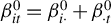
Theorem 3.5 provides pointwise inference only for each fixed i or t; it does not establish joint or simultaneous inference across multiple units or time periods. Such inference, including inference after data-dependent selection, requires additional conditions. For the cell-level slope
$\beta _{it}^{0}=\beta _{i\cdot }^{0}+\beta _{\cdot t}^{0}$
 , the natural rate of
$\hat {\beta }_{it}-\beta _{it}^{0}$
 is
$\min \{ \sqrt {N},\sqrt {T}\}$
 . If
$N/T\rightarrow \infty $
 (resp.
$ N/T\rightarrow 0$
 ), the unit-specific (resp. time-specific) error is the only leading term, and its marginal limit in Theorem 3.5 determines the limiting distribution. If
$N/T\rightarrow \kappa \in (0,\infty )$
 , both terms contribute. Because Theorem 3.5 does not guarantee their joint asymptotic normality, in this case, the expansions in Theorem 3.4 must be supplemented by the additional condition that the two leading terms are asymptotically uncorrelated.
Uniform confidence bands for the collection
$\{\beta _{i\cdot }^{0}:1\leq i\leq N\}$
 may also be of practical interest. However, the uniform asymptotic expansions in Theorem 3.4 and the marginal convergence results in Theorem 3.5 are not sufficient to justify such inference. Uniform inference requires additional conditions and theoretical results, including a uniform Gaussian approximation and the validity of an appropriate bootstrap procedure. Moreover, this problem is more challenging than that in Lu and Su (Reference Lu and Su2023), as the latent factors and factor loadings must be estimated, and their estimation errors need to be controlled uniformly alongside those of the heterogeneous slope coefficients. We therefore leave the development of uniform inference to future research.
Given the results in Theorem 3.5, it is standard to construct pointwise confidence intervals (CIs) for the elements of
$\beta _{i\cdot }^{0}$
 and
$\beta _{\cdot t}^{0}$
 . To this end, we need to estimate the parameters that appear in the variance matrices
$V_{\beta ,i\cdot }$
 and
$ V_{\beta ,\cdot t}$
 :
-
• The quantities $s_{i\cdot }^{0}$
and
$s_{\cdot t}^{0}$
can be estimated by
$\hat {\mathbf {s}}_{i\cdot }\equiv x_{i\cdot }^{\prime }M_{\hat {F }}x_{i\cdot }/T$
and
$\hat {\mathbf {s}}_{\cdot t}\equiv x_{\cdot t}^{\prime }M_{\hat {\Lambda }}x_{\cdot t}/N,$
respectively. -
• Under the additional assumption that the $\beta _{i\cdot }^{0}$
’s are independent across i,
$\Sigma _{1\beta }$
can be estimated by the sample variance of
$\hat {\beta }_{i\cdot }$
. -
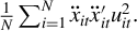
• Under the additional assumption that conditional on $(\Lambda ^{0},x_{\cdot t}), u_{it}$
’s are uncorrelated across i,
$\Phi _{\cdot t}$
equals the probability limit of
$\frac {1}{N}\sum _{i=1}^{N}\ddot {x}_{it}\ddot { x}_{it}^{\prime }u_{it}^{2}.$
An estimator of
$\Phi _{\cdot t}$
is given by
$ \hat {\Phi }_{\cdot t}\equiv \frac {1}{N}\sum _{i=1}^{N}\widehat {\ddot {x}}_{it} \widehat {\ddot {x}}_{it}^{\prime }\hat {u}_{it}^{2},$
where
$\widehat {\ddot {x}} _{it}\equiv x_{it}-x_{\cdot t}^{\prime }\hat {\Lambda }(\hat {\Lambda }^{\prime } \hat {\Lambda })^{-1}\hat {\lambda }_{i}$
. -
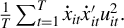
• Under the additional assumption that conditional on $(F^{0},x_{i\cdot }), u_{it}$
’s are uncorrelated across t,
$\Phi _{i\cdot }$
equals the probability limit of
$\frac {1}{T}\sum _{t=1}^{T}\dot {x}_{it}\dot {x} _{it}^{\prime }u_{it}^{2}.$
An estimator of
$\Phi _{i\cdot }$
is given by
$ \hat {\Phi }_{i\cdot }\equiv \frac {1}{T}\sum _{t=1}^{T}\widehat {\dot {x}}_{it} \widehat {\dot {x}}_{it}^{\prime }\hat {u}_{it}^{2},$
where
$\widehat {\dot {x}} _{it}\equiv x_{it}-x_{i\cdot }^{\prime }\hat {F}(\hat {F}^{\prime }\hat {F} )^{-1}\hat {f}_{t}$
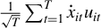
.If serial correlation is a concern, $\Phi _{i\cdot }$
represents the long-run variance of
$\frac {1}{\sqrt {T}}\sum _{t=1}^{T}\dot {x}_{it}u_{it}$
. In such cases, a heteroskedasticity-and-autocorrelation-consistent (HAC) estimator should be employed to estimate
$\Phi _{i\cdot }$
.
















Remark 3.5. The variance matrices
$\mathrm {Var}(\beta _{i\cdot }^{0})$
 and
$ \mathrm {Var}(\beta _{\cdot t}^{0})$
 can be interpreted as measures of heterogeneity in
$\beta _{i\cdot }^{0}$
 and
$\beta _{\cdot t}^{0}$
 , respectively. In practice, they can be consistently estimated using the sample variances of
$\hat {\beta }_{i\cdot }$
 and
$\hat {\beta }_{\cdot t}$
 . Under some additional conditions to ensure uniform Gaussian approximation and bootstrap validity, one may consider a formal statistical test of heterogeneity or conduct uniform confidence bands on
$\left \{ \beta _{i\cdot }^{0}\right \} $
 or
$\left \{ \beta _{\cdot t}^{0}\right \} $
 . But these certainly go beyond the scope of the article and are left for future research.
Remark 3.6. We now compare the results in Theorem 3.5 with those in Chernozhukov et al. (Reference Chernozhukov, Hansen, Liao and Zhu2026). Since we assume additive structure,
$\beta _{i\cdot }^{0}$
 and
$\beta _{\cdot t}^{0}$
 can be separately identified under the location normalization
$E(\beta _{i\cdot }^{0})=0$
 . This makes it possible to obtain the linear expansions of
$\hat { \beta }_{i\cdot }-\beta _{i\cdot }^{0}$
 and
$\hat {\beta }_{\cdot t}-\beta _{\cdot t}^{0}$
 in Theorem 3.4 and to derive the asymptotic distributions of
$\sqrt {T}(\hat {\beta }_{i\cdot }-\beta _{i\cdot }^{0})$
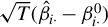 and
$ \sqrt {N}(\hat {\beta }_{\cdot t}-\beta _{\cdot t}^{0})$
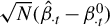 in Theorem 3.5. Given these results, we can also, under additional assumptions, study the average effects by averaging
$\beta _{i\cdot }^{0}$
 over a group of individuals or
$\beta _{\cdot t}^{0}$
 over a group of time periods. In contrast, Chernozhukov et al. (Reference Chernozhukov, Hansen, Liao and Zhu2026) assume a low-rank structure for
$\beta _{it}^{0}$
 and focus on the estimation of certain group average effects at time t. For example, one object of interest is
$\bar {\beta }_{\mathcal {G},t}^{0}=\frac {1}{\left \vert \mathcal {G} \right \vert }\sum _{i\in \mathcal {G}}\beta _{it}^{0},$
 where
$\mathcal {G}$
 is a subset of
$\left [ N\right ] $
 and
$\left \vert \mathcal {G}\right \vert $
 denotes the cardinality of the set
$\mathcal {G}$
 . Under the restrictive condition that
$\left \vert \mathcal {G}\right \vert =o(N)$
 along with some other restrictive conditions, they derive the asymptotic normality of

When
$\beta _{it}^{0}=\beta _{i\cdot }^{0}+\beta _{\cdot t}^{0}, \bar {\beta }_{\mathcal {G},t}^{0}=\frac {1}{\left \vert \mathcal {G}\right \vert }\sum _{i\in \mathcal {G}}\beta _{it}^{0}=\frac {1}{\left \vert \mathcal {G}\right \vert } \sum _{i\in \mathcal {G}}\beta _{i\cdot }^{0}+\beta _{\cdot t}^{0}.$
 In order to identify the time effect
$\beta _{\cdot t}^{0}$
 , one needs to specify
$ \mathcal {G}$
 to be
$\left [ N\right ] ,$
 which is unfortunately ruled out by the condition that
$\left \vert \mathcal {G}\right \vert =o(N)$
 in Chernozhukov et al. (Reference Chernozhukov, Hansen, Liao and Zhu2026). So the results in our article and Chernozhukov et al. (Reference Chernozhukov, Hansen, Liao and Zhu2026) are quite different from each other and they are derived under different sets of assumptions. See the next remark.
For the group average
$\bar {\beta }_{\mathcal {G},t}^{0}$
 , define
$\widehat {\bar {\beta }}_{\mathcal {G},t}\equiv |\mathcal {G} |^{-1}\sum _{i\in \mathcal {G}}\hat {\beta }_{it}$
 . Then

Conducting inference on this quantity thus requires an aggregate central limit theorem for the first term, as well as a characterization of its joint limiting behavior with the second. Under the conventional
$\sqrt {T|\mathcal {G}|}$
 rate for the first term, the relative magnitudes of
$T|\mathcal {G}|$
 and N determine which component dominates asymptotically. Furthermore, if the target of inference is a population—rather than realized—group mean, an additional central limit theorem is needed for the centered mean of the true effects
$\beta _{i\cdot }^{0}$
 ’s. These requirements are not implied by Theorems 3.4 and 3.5; rather, they play a role analogous to that of Assumption 8(vi).
Remark 3.7. The assumptions in our article are generally weaker than those in Chernozhukov et al. (Reference Chernozhukov, Hansen, Liao and Zhu2026), except for our assumption of an additive structure for
$\beta _{it}^{0}.$
 First, Chernozhukov et al. (Reference Chernozhukov, Hansen, Liao and Zhu2026) assume that the regressor
$x_{it}$
 has a strong factor structure (
$x_{it}=l_{i}^{\prime }w_{t}+e_{it}$
 ), where the zero-mean error term
$e_{it}$
 is serially independent and cross-sectionally weakly dependent. In contrast, we do not explicitly model
$x_{it}$
 and only require that the projection residual of
$x_{it}$
 —after partialling out the effect of the factors and loadings in the y-equation—is weakly dependent over
$ i $
 and t. In particular, we allow
$x_{it}$
 to contain weak factors that are not present in the y-equation. Second, Chernozhukov et al. (Reference Chernozhukov, Hansen, Liao and Zhu2026) assume that (i) the error terms in both the y- and x-equations are independent across
$t;$
 (ii) the error term in the x-equation is conditionally independent across t given the factors in the y- and x -equations, the factor component in
$\beta _{it}^{0},$
 and the error term in the y-equation, and (iii) the error term in the y-equation is conditionally independent across t given the factors in the y- and x -equations, the factor component in
$\beta _{it}^{0},$
 and the error term in the x-equation. Such (conditional) independence conditions across t are not realistic in static panels with large T, especially in empirical research. By contrast, we do not require these independence conditions; we only assume that the error terms are weakly dependent over t. Third, Chernozhukov et al. (Reference Chernozhukov, Hansen, Liao and Zhu2026) assume all loadings in the x- and y -equations and in
$\beta _{it}^{0}$
 are nonrandom and uniformly bounded. They also assume sub-Gaussianity of
$\left \{ e_{it}u_{it}\right \} $
 . We impose no similar conditions. In particular, we allow the loadings to be random and require only that all variables (including the error terms) have certain finite polynomial-order moments.
To conduct inference on the factors and factor loadings, we first introduce some notation. Define
$V=\mathrm {diag}(v_{1},\ldots ,v_{R^{0}})$
 and
$ Q=V^{1/2}\Upsilon ^{\prime }\Sigma _{\Lambda }^{-1/2}$
 , where
$ v_{1}>v_{2}>\cdots >v_{R^{0}}>0$
 are the eigenvalues of
$\Sigma _{\Lambda }^{1/2}\Sigma _{F}\Sigma _{\Lambda }^{1/2}$
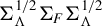 , and
$\Upsilon $
 is the corresponding matrix of eigenvectors satisfying
$\Upsilon ^{\prime }\Upsilon =\mathbb {I}_{R^{0}}$
 . Let
$\tilde {\mathbf {Y}}=\mathbf {Y}-\mathrm {mat}\!\big (X^{(1,2)}\hat {B}\big )$
 , and let
$V_{NT}$
 denote the
$R^{0}\times R^{0}$
 diagonal matrix containing the largest
$R^{0}$
 eigenvalues of
$(NT)^{-1} \tilde {\mathbf {Y}}\tilde {\mathbf {Y}}^{\prime }$
 , arranged in decreasing order. Define
$H=\big (N^{-1}\Lambda ^{0^{\prime }}\Lambda ^{0}\big )\big (T^{-1}F^{0^{\prime }}\hat {F}\big )V_{NT}^{-1}.$
 The following theorem establishes the asymptotic distributions of
$\hat {f}_{t}$
 ,
$\hat {\lambda } _{i} $
 , and the product
$\hat {\lambda }_{i}^{\prime }\hat {f}_{t}$
 .
Theorem 3.6. Suppose that Assumptions 1–6 hold and
$(\sqrt {N}/T+ \sqrt {T}/N)\log ^{2}(NT)\rightarrow 0$
 . Let
$V_{1,it}=$
 ${\lambda _{i}^{0}}^{\prime }\Sigma _{\Lambda }^{-1}\Gamma _{\cdot t} \Sigma _{\Lambda }^{-1}\lambda _{i}^{0}/N$
 and
$V_{2,it}={f_{t}^{0}}^{\prime }\Sigma _{F}^{-1}\Gamma _{i\cdot } \Sigma _{F}^{-1}f_{t}^{0}/T$
 . Then
(i)
$\sqrt {N}(\hat {f}_{t}-H^{\prime }f_{t}^{0})\overset {d}{\rightarrow } N\left (0,V^{-1}Q\Gamma _{\cdot t}Q^{\prime }V^{-1}\right ) $
 for each
$t\in \left [ T\right ] $
 ;
(ii)
$\sqrt {T}(\hat {\lambda }_{i}-H^{-1}{\lambda }_{i}^{0})\overset {d}{ \rightarrow }N\left (0,(Q^{\prime })^{-1}\Gamma _{i\cdot }Q^{-1}\right ) $
 for each
$i\in \left [ N\right ] $
 ;
(iii)
$(V_{1,it}+V_{2,it})^{-1/2}(\hat {\lambda }_{i}^{\prime }\hat {f} _{t}-\lambda _{i}^{0\prime }f_{t}^{0})\overset {d}{\rightarrow }N\left (0,1\right ) $
 for each pair
$\left (i,t\right ) \in \left [ N \right ] \times \left [ T\right ].$

Theorem 3.6 provides pointwise distribution results. It does not establish joint or simultaneous inference across multiple time periods or units. In particular, uniform inference on the factor trajectory
$\{f_{t}^{0}\}_{t\leq T}$
 under the adopted normalization (equivalently, on the rotated trajectory
$\{H^{\prime }f_{t}^{0}\}_{t\leq T}$
 ) requires additional conditions and a uniform asymptotic linear expansion for
$\hat {f}_{t}-H^{\prime }f_{t}^{0}$
 , analogous to the expansions in Theorem 3.4, together with a uniform Gaussian approximation and valid critical values for the corresponding maximum statistic. We leave the development of such uniform inference to future research.
The covariance matrices
$\Gamma _{\cdot t}$
 and
$\Gamma _{\cdot i}$
 , as in Assumption 6(v) and (vi), are different from that often appear in the factor literature. This point indicates the slow convergences of
$\hat {\beta } _{\cdot t}$
 and
$\hat {\beta }_{i\cdot }$
 enter the asymptotics of
$\hat {f} _{t} $
 and
$\hat {\lambda }_{i},$
 respectively, and both enter the asymptotic distribution of the estimator of the common component
$\lambda _{i}^{0\prime }f_{t}^{0}.$

4 ESTIMATION OF HETEROGENEOUS TREATMENT EFFECTS
In this section, we study the estimation of heterogeneous treatment effects by using the model proposed in the last section.
4.1 Basic Setup
One key application of our asymptotic results is to estimate various heterogeneous causal effects. To illustrate the main idea, we consider a simple setup where we have
$N=N_{1}+N_{2}$
 individuals where the first
$ N_{1} $
 individuals
$\left (i\in \lbrack N_{1}]\right ) $
 never receive any treatment, and the last
$N_{2}$
 individuals
$(i\in \left [ N\right ] \backslash \left [ N_{1}\right ] \equiv \{N_{1}+1,\ldots ,N\})$
 receive treatment at some potentially different time points. We focus on the case where once a unit adopts the treatment, it stays treated afterward. We denote by
$T_{0,i}$
 and
$T_{1,i}$
 the number of control and treated time periods for unit i such that
$T_{0,i}+T_{1,i}=T.$
 If individual i never receives treatment, then
$T_{0,i}=T$
 and
$T_{1,i}=0$
 . Following the literature of the potential outcome framework, we use
$y_{it}^{1}$
 and
$ y_{it}^{0}$
 to denote the potential outcome for individual i who receives and does not receive the treatment at time t, respectively. Let
$y_{it}$
 be the observed outcome:
$y_{it}=y_{it}^{1}d_{it}+y_{it}^{0}\left (1-d_{it}\right ) ,$
 where
$d_{it}=\mathbf {1}\{$
 individual i receives treatment at time
$t\}$
 is the treatment indicator. Let
$\mathcal {D} ^{0}\equiv \{(i,t)\mid d_{it}=0,(i,t)\in \lbrack N]\times \lbrack T]\}$
 and
$ \mathcal {D}^{1}\equiv ([N]\times \lbrack T])\backslash \mathcal {D}^{0}$
 . Thus, we observe
$y_{it}^{0}$
 ’s for
$(i,t)\in \mathcal {D}^{0}$
 and
$ y_{it}^{1}$
 ’s for
$(i,t)\in \mathcal {D}^{1}$
 , respectively.
The individual treatment effect measures the difference between the treated and control outcome:

We do not impose any assumptions on
$y_{it}^{1}$
 and therefore
$ \tau _{it}$
 . In particular,
$y_{it}^{1}$
 does not need to follow a model like that for
$y_{it}^{0}$
 .
$\tau _{it}$
 can be heterogeneous across both i and t and it does not necessarily have a factor structure as assumed in Xiong and Pelger (Reference Xiong and Pelger2023). We are only interested in the treatment effect on the treated, that is,
$\tau _{it}$
 for
$(i,t)\in \mathcal {D}^{1}$
 . For them, we directly observe
$y_{it}^{1},$
 and therefore we only need to model
$ y_{it}^{0}.$
 We assume that
$y_{it}^{0}$
 is generated via the following data-generating process (DGP):

where
$x_{it}$
 ,
$\beta _{i\cdot }^{0},\beta _{\cdot t}^{0}, \lambda _{i}^{0}, f_{t}^{0},$
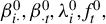 and
$u_{it}$
 are as defined in the last section. As we do not observe all
$y_{it}^{0}$
 ’s for
$(i,t)\in \lbrack N]\times \lbrack T]$
 , model (4.1) assists in imputing unobserved
$y_{it}^{0}$
 ’s.
Nevertheless, identification of the counterfactual untreated outcomes relies on model (4.1), which is assumed to hold for all
$ (i,t)$
 , including treated cells for which
$y_{it}^{0}$
 is counterfactual. In particular, conditional on
$x_{it}$
 , the time-specific slope
$\beta _{\cdot t}^{0}$
 and common factor
$f_{t}^{0}$
 are shared across all units. Thus, rather than dispensing with a parallel-trends-type restriction, our conditional factor model for untreated outcomes imposes a factor-augmented stability condition in the same spirit as the conditional parallel-trends assumption in the staggered difference-in-differences literature.
Let
$\mathcal {G}_{t}\equiv \left \{ i\in \left [ N\right ] \backslash \left [ N_{1}\right ] ,\text { }d_{it}=1\right \} $
 and
$\bar {T}_{1}=\frac {1}{N_{2}} \sum _{i=N_{1}+1}^{N}T_{1,i}.$
 Let
$\left \vert \mathcal {G}_{t}\right \vert $
 denote the cardinality of the set
$\mathcal {G}_{t},$
 that is, the number of individuals who receive treatment at time
$t.$
 In the following, we consider different levels of ATT:
-
1. Average treatment effect on the treated for i: $\tau _{i\cdot }= \frac {1}{T_{1,i}}\sum _{t=T_{0,i}+1}^{T}\tau _{it}.$
-
2. Average treatment effect on the treated at time $t:\tau _{\cdot t}= \frac {1}{\left \vert \mathcal {G}_{t}\right \vert }\sum _{i\in \mathcal {G} _{t}}\tau _{it}.$
-
3. Aggregate average treatment effect on the treated: $\bar {\tau }=\frac {1 }{N_{2}\bar {T}_{1}}\sum _{i=N_{1}+1}^{N}\sum _{t=T_{0,i}+1}^{T}\tau _{it}.$



Since we do not make any assumption on
$\tau _{it},$
 it is impossible to eliminate the effect of
$u_{it}$
 on the estimator of
$\tau _{it}$
 for a single cross-sectional unit at a time period. This motivates the above consideration of ATT. Of course, one can also consider other forms of treatment effects, say, weighted treatment effects, or treatment effects for certain selected groups of individuals or time periods. For each of the above three types of treatment effects, we derive the asymptotic distributions based on which we can test for the null hypothesis of no causal effects.
Nevertheless, if one would like to assume that
$u_{it}$
 has the same distribution over either i or
$t,$
 or both, we argue below that it is still possible to make inference on
$\tau _{it}$
 by relying on some other method.
4.2 Estimation of Heterogeneous Treatment Effects
Due to the presence of the two-dimensional unobserved slope heterogeneity in (4.1), we assume that both
$N_{1}$
 and T pass to infinity. This enables us to apply the asymptotic results in Section 3 to derive the asymptotic properties of certain estimators based on the data
$ \left \{ \left (y_{it},x_{it}\right ) \right \} _{i\in \left [ N_{1}\right ] ,t\in \left [ T\right ] }.$
 Then we can propose an estimator for the counterfactual outcome
$y_{it}^{0}$
 for
$i=N_{1}+1,\ldots ,N$
 and
$ t=T_{0,i}+1,\ldots ,T,$
 based on model (4.2) below.
Algorithm 2 (Estimation of the counterfactual outcome
$y_{it}^{0}$
for
$(i,t)\in \mathcal {D}^1$
)


-
1. Run the nuclear-norm-regularized estimation based on the model
(4.2) $$ \begin{align} y_{it}=\left(\beta _{i\cdot }^{0}+\beta _{\cdot t}^{0}\right) ^{\prime }x_{it}+\lambda _{i}^{0\prime }f_{t}^{0}+u_{it}\ \ \ \text{ for }(i,t)\in \lbrack N_{1}]\times \lbrack T]. \end{align} $$
Obtain the preliminary estimator of the common component $\Theta , $
which is now a
$T\times N_{1}$
matrix, based on which we obtain a consistent estimator of
$R^{0}.$
Obtain the post-nuclear norm iterated estimators of
$ \left \{ \beta _{i\cdot }^{0},\lambda _{i}^{0}\right \} _{i\in \left [ N_{1} \right ] }$
and
$\left \{ \beta _{\cdot t}^{0},f_{t}^{0}\right \} _{t\in \left [ T\right ] },$
denoted as
$\{\hat {\beta }_{i\cdot },\hat {\lambda }_{i}\}_{i\in \left [ N_{1}\right ] }$
and
$\{\hat {\beta }_{\cdot t},\hat {f}_{t}\}_{t\in \left [ T\right ] }.$
-
2. Given $\{\hat {\beta }_{\cdot t},\hat {f}_{t}\}_{t\in \left [ T\right ] },$
we estimate
$\left \{ \beta _{i\cdot }^{0},\lambda _{i}^{0}\right \} _{i\in \left [ N\right ] \backslash \left [ N_{1}\right ] }$
by running a time-series regression for each
$i\in \left [ N\right ] \backslash \left [ N_{1}\right ] $
using the data
$\left \{ y_{it},x_{it}^{\prime }\right \} _{t\in \lbrack T_{0,i}]}:$
$$ \begin{align*} y_{it}-\hat{\beta}_{\cdot t}^{\prime }x_{it}=\beta _{i\cdot }^{0\prime }x_{it}+\lambda _{i}^{0\prime }\hat{f}_{t}+e_{it},\ \ \ \text{ for }t\in \lbrack T_{0,i}], \end{align*} $$where $e_{it}$
signifies the regression error that includes the parameter estimation error (PEE) from the early stage regression. Let
$\hat {\beta } _{i\cdot }$
and
$\hat {\lambda }_{i}$
denote the resulting estimators of
$ \beta _{i\cdot }^{0}$
and
$\lambda _{i}^{0},$
respectively.
-
3. Estimate the counterfactual outcome $y_{it}^{0}$
as
$\hat {y}_{it}^{0}=(\hat {\beta }_{i\cdot }+\hat {\beta }_{\cdot t})^{\prime }x_{it}+\hat {\lambda } _{i}^{\prime }\hat {f}_{t}$
for
$(i,t)\in \mathcal {D}^{1}.$


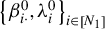
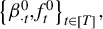


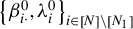

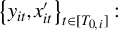




Let
$\hat {\tau }_{it}=y_{it}-\hat {y}_{it}^{0}$
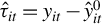 for
$(i,t)\in \mathcal {D}^{1}.$
 $\hat {\tau }_{it}$
 is an estimator of
$\tau _{it}$
 that is asymptotically unbiased but generally inconsistent. Then we can estimate
$\tau _{i\cdot },$
 $\tau _{\cdot t}$
 , and
$\bar {\tau }$
 as follows:

In the next section, we will study the asymptotic properties of
$\hat {\tau } _{i\cdot }, \hat {\tau }_{\cdot t},$
 and
$\hat {\tau }$
 under some regularity conditions, based on which one can make valid inferences on
$\tau _{i\cdot }, \tau _{\cdot t}$
 , and
$\bar {\tau }.$

For notational simplicity, here we consider the staggered treatment timing. Our approach can actually handle any irregular treatment pattern as long as the untreated period is reasonably long for the treated units. In this case, we simply run a time-series regression using the data from the untreated period in Step 2 of Algorithm 2 and estimate the counterfactual outcome for the treated periods in Step 3. Neither step requires regularly spaced time-series data.
4.3 Asymptotic Distributions
In this section, we study the asymptotic distributions of
$\hat {\tau } _{i\cdot }, \hat {\tau }_{\cdot t}$
 , and
$\hat {\tau }.$
 We first state the potential outcome assumptions formally.
Assumption 7. (Conditions for Potential Outcomes)
(i) The untreated and treated potential outcomes,
$y_{it}^{0}$
 and
$y_{it}^{1},$
 are given by

where
$i\in \left [ N\right ] $
 and
$t\in \left [ T\right ] .$

(ii)
$E\left (u_{it}|x_{it},\beta _{i\cdot }^{0},\beta _{\cdot t}^{0},F^{0},\Lambda ^{0},{{\{d_{is}\}_{s\leq t}}}\right ) =0.$

Assumption 7(i) is common in the synthetic control literature. For example, it is similar to Assumption 1 in Ferman and Pinto (Reference Ferman and Pinto2021) and Assumption 1 in Xu (Reference Xu2017) except that our model specification is more general with covariates and we allow for two-dimensional heterogeneity in the slope coefficients. Assumption 7(ii) strengthens the exogeneity Assumption 6(i) by requiring that
$u_{it}$
 be mean-independent of the treatment history
$ \{d_{is}\}_{s\leq t}$
 . This is similar to Assumption 3 in Ferman and Pinto (Reference Ferman and Pinto2021) and Assumption 2 in Xu (Reference Xu2017).
We now state some technical assumptions. With a little bit abuse of notation, we continue to use
$\hat{\boldsymbol{B}}_{k,T}=$
 diag(
$\hat {\beta } _{k,\cdot 1}, \ldots ,\hat {\beta }_{k,\cdot T}$
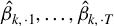 ) and
$\hat{\boldsymbol{B}} _{k,N_{1}}=$
 diag(
$\hat {\beta }_{k,1\cdot },\ldots ,\hat {\beta }_{k,N_{1}\cdot }$
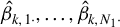 ) to denote estimators of
$\boldsymbol{\dot {B}}_{k,T}=$
 diag
$(\dot {\beta }_{k,\cdot 1}, \ldots ,\dot {\beta }_{k,\cdot T})$
 and
$\boldsymbol{\dot {B}}_{k,N_{1}}=$
 diag(
$ \dot {\beta }_{k,1\cdot },\ldots , \dot {\beta }_{k,N_{1}\cdot }$
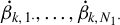 ) based on the data
$\left \{ \left (y_{it},x_{it}\right ) \right \} _{i\in \left [ N_{1}\right ] ,t\in \left [ T\right ] }.$
 The corresponding matrices
$\mathbf {Y}$
 (or
$ \mathbf {X}_{k})$
 and B (or
$\hat {B})$
 are now of dimensions
$ T\times N_{1}$
 and
$\left (N_{1}+T-1\right ) K\times 1,$
 respectively. Let
$ \boldsymbol{\tilde {Y}=} \mathbf {Y}-\sum _{k=1}^{K}(\hat{\boldsymbol{B}}_{k,T} \mathbf {X}_{k}+\mathbf {X}_{k}\hat{\boldsymbol{B}}_{k,N_{1}})=\mathbf {Y}-$
 mat
$ (X^{\left (1,2\right ) }\hat {B}).$
 Let
$V_{N_{1}T}$
 be the
$R^{0}\times R^{0}$
 diagonal matrix of the first
$R^{0}$
 largest eigenvalues of
$\left (N_{1}T\right ) ^{-1}\boldsymbol{\tilde {Y}\tilde {Y}}^{\prime }$
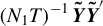 in decreasing order along its main diagonal line. Let
$H =(N_{1}^{-1}\Lambda ^{0\prime }\Lambda ^{0})(T^{-1}F^{0\prime }\hat {F})V_{N_{1}T}^{-1},$
 where
$\Lambda ^{0}\equiv \Lambda _{N_{1}}^{0}\equiv \lbrack \lambda _{1}^{0},\ldots ,\lambda _{N_{1}}^{0}]^{\prime }.$
 Let
$z_{it}=\left (x_{it}^{\prime },f_{t}^{0\prime }H\right ) ^{\prime }$
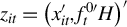 and
$\bar {z}_{it}=\left (x_{it}^{\prime },f_{t}^{0\prime }\right ) ^{\prime }.$
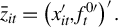 Similarly,
$\mathbf {x}_{\cdot t}=[x_{1t},\ldots ,x_{N_{1}t}]^{\prime }$
 is now an
$N_{1}\times K$
 matrix. Let
$ \mathbb {S}_{1}\in \mathbb {R}^{K\times \left (K+R^{0}\right ) }$
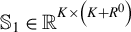 and
$\mathbb {S }_{2}\in \mathbb {R}^{R^{0}\times \left (K+R^{0}\right ) }$
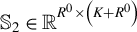 denote selection matrices such that
$\mathbb {S}_{1}A$
 and
$\mathbb {S}_{2}A$
 select the first
$ K$
 rows and the last
$R^{0}$
 rows of
$A,$
 respectively. Define

where
${\mathrm {blkdiag}}\left (\cdot \right ) $
 signifies a block diagonal matrix. Let
$\underline {T}_{0}=\min _{i\in \left [ N\right ] \backslash \left [ N_{1}\right ] }T_{0,i}$
 and
$\bar {T}_{1}=\frac {1}{N_{2}}\sum _{i=N_{1}+1}^{N}T_{1,i}.$
 We add the following assumption.
Assumption 8.
-
(i) $\max _{i\in \left [ N\right ] \backslash \left [ N_{1}\right ] }\{\frac {1}{T_{0,i}}E||\sum _{t=1}^{T_{0,i}}(x_{it}-\mu _{i\cdot ,x})||^{2}+ \frac {1}{T_{1,i}}E||\sum _{t=T_{0,i}+1}^{T}(x_{it}-\mu _{i\cdot ,x})||^{2} + \frac {1}{T_{1,i}}||\sum _{t=T_{0,i}+1}^{T} (f_{t}^{0}-\mu _{f})||^{2}+ \frac {1}{N_{2}\bar {T}_{1}}||\sum _{j,k=N_{1}+1}^{N}\sum _{t,s=T_{0,i}+1}^{T}E(\lambda _{j}^{0}\lambda _{k}^{0\prime }u_{jt}u_{ks})||\} \leq C;$
-
(ii) $\max _{t\in \left [ T\right ] }\{||\frac {1}{N_{1}}\mathbf {x}_{\cdot t}^{\prime }\mathbb {M}_{\Lambda ^{0}}\mathbf {x}_{\cdot t}-\mathbf {s}_{\cdot t}^{0}||+||\frac {1}{N_{1}}\sum _{j=1}^{N_{1}}x_{jt}\lambda _{j}^{0\prime }-\mu _{\cdot t,x\lambda }||+\left \Vert \hat {\pi }_{t,x\lambda }-\pi _{t,x\lambda }\right \Vert \}=O_{P}(N_{1}^{-1/2}\log T);$
-
(iii) $\max _{i\in \left [ N\right ] \backslash \left [ N_{1}\right ] }||\frac {1}{ T_{0,i}}\sum _{t=1}^{T_{0,i}}z_{it}z_{it}^{\prime }-S_{i}||=O_{P}[(\underline { T}_{0}/\log N)^{-1/2}]$
for some
$S_{i}>0;$
-
(iv) for each i, $\frac {1}{\sqrt {T_{1,i}}} \sum _{t=T_{0,i}+1}^{T}u_{it}\overset {d}{\rightarrow }N(0,\sigma _{i\cdot ,u}^{2})$
and
$\frac {1}{\sqrt {T_{1,i}}}\sum _{t=T_{0,i}+1}^{T}z_{it}u_{it} \overset {d}{\rightarrow }N(0,\Omega _{i,zu})$
; -
(v) for each $t\in \left [ T\right ] \backslash \left [ \min _{i\in \left [ N\right ] }T_{0,i}\right ] $
, as
$|\mathcal {G}_{t}|\rightarrow \infty ,$
$\frac {1}{\sqrt {\left \vert \mathcal {G}_{t}\right \vert }}\sum _{i\in \mathcal {G}_{t}}u_{it}\overset {d}{\rightarrow }N\left (0,\sigma _{\cdot t,u}^{2}\right ) $
and
$\frac {1}{\sqrt {N_{1}}}\sum _{j=1}^{N_{1}}[\nu _{\cdot t,x\lambda }^{\prime } \left (\mathbf {s}_{\cdot t}^{0}\right ) ^{-1} (x_{jt}-\pi _{t,x\lambda }^{\prime }\lambda _{j}^{0})-\mu _{\lambda }^{\prime }\Sigma _{\Lambda }^{-1}\lambda _{j}^{0}]u_{jt} \overset {d}{\rightarrow }N(0,\Xi _{\cdot t})$
; -
(vi) $\frac {1}{\sqrt {N_{2}\bar {T}_{1}}}\sum _{i=N_{1}+1}^{N} \sum _{t=T_{0,i}+1}^{T}u_{it}\overset {d}{\rightarrow }N\left (0,\sigma _{u}^{2}\right ) $
and
$\frac {1}{\sqrt {N_{2}}}\sum _{i=N_{1}+1}^{N}\alpha _{i\cdot ,T}\frac {1}{\sqrt {T_{0,i}}}\sum _{t=1}^{T_{0,i}}z_{it}u_{it} \overset {d}{\rightarrow }N\left (0,\Xi \right ) ;$
-
(vii) $\max _{i\in \left [ N\right ] }\{||(N_{1}T)^{-1/2}\sum _{t=1}^{T} \sum _{j=1}^{N_{1}}\lambda _{j}^{0}u_{jt}x_{it}^{\prime }||+ ||(N_{1}T)^{-1/2}\sum _{t=1}^{T}\zeta _{it}^{\prime }(\mathbf {s}_{\cdot t}^{0})^{-1}\mathbf {x}_{\cdot t}^{\prime }$
$\mathbb {M}_{\Lambda ^{0}}\mathbf {u} _{\cdot t}||\}=O_{P}(\log \left (N_{1}T\right ) )$
for
$\zeta _{it}=\nu _{\cdot t,x\lambda }, \mu _{\cdot t,x\lambda }x_{k,it},$
and
$ x_{it}x_{k,it}$
with
$k\in \lbrack K].$

















Assumption 8 imposes some conditions of
$\left \{ x_{it},u_{it},\lambda _{i}^{0},f_{t}^{0}\right \} $
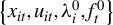 that can be verified under some primitive conditions. Assumption 8 contains three types of asymptotic conditions. First, parts (iv) and (v) impose pointwise convergence conditions. These conditions support parts (i) and (ii), respectively, of Theorem 4.1. Second, part (vi) imposes aggregate convergence conditions jointly over treated units and post-treatment periods and is needed only for the overall average estimator in Theorem 4.1(iii). Third, parts (i)–(iii) and (vii) impose uniform bounds over the relevant unit and time indices. In establishing Theorem 4.1(iii), the aggregate limits in part (vi), together with these uniform bounds, control the accumulation of the leading terms and estimation remainders when averaging over both dimensions.
The following theorem states the asymptotic distributions of
$\hat {\tau } _{i\cdot }, \hat {\tau }_{\cdot t}$
 , and
$\hat {\tau }.$

Theorem 4.1. Suppose Assumptions 1–8 hold for
$ \left \{ \left (y_{it},x_{it}\right ) \right \} _{i\in \left [ N_{1}\right ] ,t\in \left [ T\right ] }$
 with obvious changes to take into account the change in the sample size. Suppose that
$(\sqrt {N_{1}}/T+\sqrt {T}/N_{1})\log ^{2}(N_{1}T)\rightarrow 0$
 and
$\frac {T_{0,i}}{T}\rightarrow r_{i}\in (0,1]$
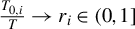 as
$(N_{1},T)\rightarrow \infty $
 . Then
(i) For each fixed treated unit i, as
$T_{1,i}\rightarrow \infty ,$


where
$\Xi _{i\cdot }\equiv (\mu _{i\cdot ,x}^{\prime }\mathbb {S}_{1}+\mu _{f}^{\prime }Q^{-1}\mathbb {S}_{2})S_{i}^{-1}\Omega _{i,zu}S_{i}^{-1}(\mathbb {S}_{1}^{\prime }\mu _{i\cdot ,x}+\mathbb {S}_{2}^{\prime }(Q^{-1})^{\prime }\mu _{f}).$

(ii) For each fixed time period
$t\in \left [ T\right ] \backslash \left [ \min _{i\in \left [ N\right ] }T_{0,i}\right ] $
 , as
$ \left \vert \mathcal {G}_{t}\right \vert \rightarrow \infty $
 and
$\frac { \left \vert \mathcal {G}_{t}\right \vert }{N_{1}}\rightarrow r_{\cdot t}\in \lbrack 0,\infty ),$


(iii) As
$\bar {T}_{1}\rightarrow \infty $
 and
$N_{2}$
 is either fixed or diverges to infinity such that
$N_{2}=o(\min (N_{1}, \underline {T} _{0}/\log N, \delta _{N_{1}T}^{4}/\{\bar {T}_{1}[\log (N_{1}T)]^{2}\})),$


Theorem 4.1 studies the asymptotic distributions of
$\hat {\tau } _{i\cdot }, \hat {\tau }_{\cdot t}$
 , and
$\hat {\tau }.$
 To make inferences, we need to consistently estimate the asymptotic variances. Let
$\hat {z} _{it}=(x_{it}^{\prime },\hat {f}_{t}^{\prime })^{\prime }$
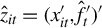 for
$(i,t)\in [N]\times [T]$
 and
$\hat {u}_{it}=y_{it}-x_{it}^{ \prime }(\hat {\beta } _{i\cdot }+\hat {\beta }_{\cdot t})-\hat {\lambda } _{i}^{\prime }\hat {f}_{t}$
 for
$(i,t)\in \mathcal {D}^0$
 .
Case (1). Since
$\sigma _{i\cdot ,u}^{2}$
 and
$\Omega _{i,zu}$
 denote the long-run variance of
$\left \{ u_{it}\right \} $
 and
$ \left \{ z_{it}u_{it}\right \} ,$
 it is standard to use
$\left \{ \hat {u} _{it}\right \} $
 and
$\left \{ \hat {z}_{it}\hat {u}_{it}\right \} $
 to estimate them by HAC estimators. The main difficulty here lies in the fact that the above definition of
$\hat {u}_{it}$
 only works for the pre-treatment period when individual i receives the treatment in period
$t.$
 When
$(i,t)\in \mathcal { D}^{1}$
 , we cannot consistently estimate
$u_{it}$
 . Under the covariance stationarity of
$\left \{ \left (u_{it},\bar {z}_{it}u_{it}\right ) ,t\geq 1\right \} ,$
 we can estimate
$\sigma _{i\cdot ,u}^{2}$
 and
$\Omega _{i,zu}$
 , respectively, by

where
$w\left (\cdot \right ) $
 is a kernel function and
$m=m_{T}$
 is a truncation parameter. Of course, if
$\left \{ (u_{it},\bar {z} _{it}u_{it})\right \} $
 share the same variance–covariance matrix across
$ i\in \left [ N\right ] \backslash \left [ N_{1}\right ] ,$
 one can pool over the treated cross-sectional units to estimate the above variances more accurately in finite samples. Then, we can estimate the asymptotic variance of
$\sqrt {T_{1,i}}\left (\hat {\tau }_{i\cdot }-\tau _{i\cdot }\right ) $
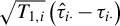 by

where
$\hat {\mu }_{i\cdot ,x}=\frac {1}{T_{1,i}}\sum _{t=T_{0,i}+1}^{T}x_{it},$
 $\hat {\mu }_{f}=\frac {1}{T}\sum _{t=1}^{T}\hat {f}_{t},$
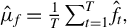 and
$\hat {S} _{i,T_{0,i}}=\frac {1}{T_{0,i}}\sum _{t=1}^{T_{0,i}}\hat {z}_{it}\hat {z} _{it}^{\prime }.$
 Alternatively, under the covariance stationarity of
$ \left \{ \bar {z}_{it},t\geq 1\right \} ,$
 we can also use the following estimators
$\tilde {\mu }_{i\cdot ,x}=\frac {1}{T} \sum _{t=1}^{T}x_{it}$
 and
$\tilde {S}_{i}=\frac {1}{T}\sum _{t=1}^{T}\hat {z} _{it}\hat {z}_{it}^{\prime }$
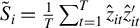 to replace
$\hat {\mu }_{i\cdot ,x}$
 and
$\hat {S} _{i,T_{0,i}},$
 respectively.
Case (2). Under the condition that
$\left \{ u_{it},x_{it},\lambda _{i}^{0}\right \} $
 are independent across
$i,$
 we can estimate
$\sigma _{\cdot t,u}^{2}$
 and
$\Xi _{\cdot t}$
 , respectively, by

where
$\hat{\boldsymbol{s}}_{\cdot t}=\frac {1}{N_{1}}\mathbf {x}_{\cdot t}^{\prime }\mathbb {M}_{\hat {\Lambda }}\mathbf {x}_{\cdot t}, \hat {\mu } _{\lambda }=\frac {1}{N_{1}}\sum _{j=1}^{N_{1}}\hat {\lambda }_{j}$
 , and
$\hat { \nu }_{\cdot t,x\lambda }=\frac {1}{\left \vert \mathcal {G}_{t}\right \vert } \sum _{i\in \mathcal {G}_{t}}[x_{it}-$
 $\mathbf {x}_{\cdot t}^{\prime }\hat {\Lambda }(\hat {\Lambda }^{\prime }\hat {\Lambda })^{-1}\hat {\lambda }_{i}].$
 Then we can estimate the asymptotic variance of
$\sqrt {\left \vert \mathcal {G} _{t}\right \vert }\left (\hat {\tau }_{\cdot t}-\tau _{\cdot t}\right ) $
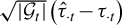 by

Case (3). We can estimate
$\sigma _{u}^{2}$
 and
$\Xi $
 by the panel HAC estimators
$\hat {\sigma }_{u}^{2}$
 and
$\hat {\Xi },$
 respectively, where

As in Case (1), here we use the covariance stationarity of
$\left \{ \left (u_{it},\bar {z}_{it}u_{it}\right ) ,t\geq 1\right \} $
 to obtain
$\hat {\sigma } _{u}^{2}.$
 Then we can estimate the asymptotic variance of
$\sqrt {N_{2}\bar { T }_{1}}\left (\hat {\tau }-\bar {\tau }\right ) $
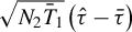 by

Despite the fact that
$\hat {\tau }_{it}$
 is generally inconsistent, we can still construct valid CIs for
$\tau _{it}$
 under certain stationarity conditions on
$\left \{ u_{it}\right \} .$
 This is because
$\hat {\tau }_{it}=\tau _{it}+u_{it}+o_{P}\left (1\right ) $
 by Lemma A.7(i) in Section A.2 of the Supplementary Material. For example, if
$ \left \{ u_{it}\right \} $
 for the treated units are strictly stationary over both i and t, we can establish the 100
$\left (1-\alpha \right ) \%$
 CI for
$\tau _{it}$
 as
$\left [ \hat {\tau }_{it}+\hat {q} _{u,\alpha /2},\hat {\tau }_{it}+\hat {q}_{u,1-\alpha /2}\right ] ,$
 where, for example,
$\hat {q}_{u,\alpha /2}$
 denotes the
$\alpha /2$
 -sample quantile of
$\{- \hat {u}_{it}, i\in \left [ N\right ] \backslash \left [ N_{1}\right ] , t\in \left [ T_{0,i}\right ] \}.$
 Similarly, if we further impose strict stationarity for
$\left \{ u_{it}\right \} $
 for both the control units and treated units, we can use the sample quantiles of the combination of
$\{- \hat {u}_{it},\,i\in \left [ N\right ] \backslash \left [ N_{1}\right ] , t\in \left [ T_{0,i}\right ] \}$
 and
$\{-\hat {u}_{it},i\in \left [ N_{1}\right ] ,t\in \left [ T\right ] \}.$
 Alternatively, we can apply the permutation test proposed by Chernozhukov et al. (Reference Chernozhukov, Wüthrich and Zhu2021) to conduct inference for
$\tau _{it} $
 .
5 MONTE CARLO SIMULATIONS
5.1 Data-Generating Processes and Implementations
To examine the finite sample performance of our estimation method, we conduct simulations with four DGPs. For all DGPs, the untreated outcome is generated as in models (1.1) and (1.2), and the treatment effect (TE),
$\tau _{it}$
 is randomly drawn from the
$N\left (1,1\right ) $
 distribution.
We first consider simple DGPs 1 and 2 to illustrate the main idea of our approach. In both DGPs,
$x_{it}$
 is a scalar, the number of factors (
$R^{0}$
 ) is 2,
$x_{it}$
 and
$u_{it}$
 are all generated from independent and identically distributed (IID)
$N\left (0,1\right ) ,$
 and
$\lambda _{i}^{0}$
 and
$f_{t}^{0}$
 are drawn from IID
$\ N\left (0,\mathbb {I}_{2}\right ) .$
 We consider two different cases for
$\beta _{i\cdot }^{0}$
 and
$\beta _{\cdot t}^{0}.$
 In DGP 1 (heterogeneous case),
$\beta _{i\cdot }^{0}$
 and
$\beta _{\cdot t}^{0}$
 are IID
$N\left (0,1\right ) $
 and
$N\left (1,1\right ) $
 random variables. In DGP 2 (homogeneous case),
$\beta _{i\cdot }^{0}=0$
 and
$ \beta _{\cdot t}^{0}=1$
 for all i and
$t.$
 Note that for DGP 2, our proposed model is over-fitted, therefore we can examine the effect of over-fitting by comparing it with the traditional homogeneous model where
$ (\beta _{i\cdot }^{0}+\beta _{\cdot t}^{0})$
 is restricted to be a constant.
DGPs 3 and 4 are more realistic. In both DGPs, there are two covariates
$ x_{it}=\left (x_{1,it},x_{2,it}\right ) ^{\prime }$
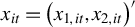 and two factors
$ f_{t}^{0}=\left (f_{t,1}^{0},f_{t,2}^{0}\right ) ^{\prime }$
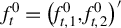 . Correspondingly, define
$\lambda _{i}^{0}=\left (\lambda _{i,1}^{0},\lambda _{i,2}^{0}\right ) ^{\prime }, \beta _{i\cdot }^{0}=\left (\beta _{1,i\cdot }^{0},\beta _{2,i\cdot }^{0}\right ) ^{\prime }$
 , and
$\beta _{\cdot t}^{0}=\left (\beta _{1,\cdot t}^{0},\beta _{2,\cdot t}^{0}\right ) ^{\prime }.$
 The details of the specifications are as follows:

$v_{t,1}, v_{t,2}, v_{it,3}, v_{it,4}, \lambda _{i,1}^{0},$
 and
$ \lambda _{i,2}^{0}$
 are drawn from IID
$N\left (0,\mathbb {I}_{6}\right ) $
 and
$v_{it,5}$
 is IID random variable from the distribution of
$\chi ^{2}\left (1\right ) -1. \beta _{1,i\cdot }^{0}$
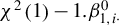 and
$\beta _{1,\cdot t}^{0} $
 are IID
$N\left (0,1\right ) $
 and
$N\left (1,1\right ) $
 random variables, and
$\beta _{2,i\cdot }^{0}=0$
 and
$\beta _{2,\cdot t}^{0}=1$
 for all i and
$t.$
 Therefore, the slope coefficient of
$x_{1,it}$
 is heterogeneous and that of
$x_{2,it}$
 is homogeneous. The difference between DGPs 3 and 4 lies in
$\rho .$
 In DGP 3,
$\rho =0,$
 therefore, there is no serial correlation in
$x_{1,it}, f_{t,1}^{0}, f_{t,2}^{0}$
 , and
$u_{it}.$
 In DGP 4,
$\rho =1/3,$
 so
$x_{1,it}, f_{t,1}^{0}, f_{t,2}^{0}$
 , and
$ u_{it}$
 are all serially correlated. Note that DGP 4 is the most complicated where the error term is conditionally heteroskedastic and serially correlated.
For DGPs 1–3, we use the White-type estimator for the variance terms to conduct inference. To improve the finite-sample performance, we impose the condition that the treated data are stationary along both cross-sectional and time dimensions. For DGP 4, we use an HAC-type estimator for the variance. It is well known that the performance of the standard HAC estimator can be poor when the time-series dimension is short (e.g., see the survey paper by Lazarus et al., Reference Lazarus, Lewis, Stock and Watson2018). To partially address this issue, we impose the stationarity of both treated and control data, and also apply a pre-whitening (PW) procedure as in Andrews and Monahan (Reference Andrews and Monahan1992) and Lu and Su (Reference Lu and Su2023). We use the growth ratio method of Ahn and Horenstein (Reference Ahn and Horenstein2013) to determine the number of factors in the initial nuclear norm regularized estimation procedure, as it outperforms singular value thresholding in our simulations and does not depend on any tuning parameter other than the maximum number of factors allowed. We set the tuning parameter as
$\gamma _{NT}=0.5\max (N_{1}^{-1/2},T^{-1/2}),$
 following Miao et al. (Reference Miao, Phillips and Su2023). We consider different combinations of
$N_{1}$
 and T:
$\left (N_{1},T\right ) =\left (40,40\right ) , \left (40,80\right ) , \left (80,40\right ) , \left (80,80\right ), $
 and
$\left (120,120\right ) .$
 We let
$N_{2}=0.25N_{1}$
 and
$T_{0i}=T_{1i}=0.5T.$
 The number of replications is 250.
5.2 Simulation Results
We first report the performance of our key Step 1 in Algorithm 2, where we use the data of control units to estimate
$\{\beta _{i\cdot }^{0},\lambda _{i}^{0}\}_{i\in \left [ N_{1}\right ] }$
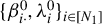 and
$\{\beta _{\cdot t}^{0},f_{t}^{0}\}_{t\in \left [ T\right ] }.$
 We define the true slope coefficient as
$\beta _{it}^{0}=\beta _{i\cdot }^{0}+\beta _{\cdot t}^{0}$
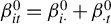 and the true factor component as
$\theta _{it}^{0}=\lambda _{i}^{0\prime }f_{t}^{0}.$
 Correspondingly, define their estimators as
$\hat {\beta }_{it}= \hat {\beta }_{i\cdot }+\hat {\beta }_{\cdot t}$
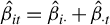 and
$\hat {\theta }_{it}=\hat { \lambda }_{i}^{\prime }\hat {f}_{t},$
 respectively. For ease of reporting, we only present the results for the slope coefficient of the first covariates for DGPs 3 and 4, where there are two covariates. Table 1 reports the mean squared errors (MSEs) of
$\hat {\beta }_{1,it}$
 (the first element of
$\hat {\beta }_{it}$
 ) and the correlation between
$\hat {\beta }_{1,it}$
 and
$ \beta _{1,it}^{0}$
 .Footnote
4
Specifically, we define

and average both measures over 250 replications. Table 1 also reports the MSEs of
$\hat {\theta }_{it}$
 and the correlation between
$\hat { \theta }_{it}$
 and
$\theta _{it}^{0}$
 , which are defined as

averaging over 250 replications. Table 1 shows that our estimation procedure in Step 1 works well. The correlations between
$\hat { \beta }_{1,it}$
 and
$\beta _{1,it}^{0}$
 and between
$\hat {\theta }_{it}$
 and
$ \theta _{it}^{0}$
 are all above 0.97 for DGPs 1 and 2, and all above 0.85 for DGPs 3 and 4. The MSEs of
$\hat {\beta }_{1,it}$
 and
$\hat {\theta }_{it}$
 decrease with
$N_{1}$
 and
$T,$
 as expected. Our method can determine the correct number of factors with a high probability. For simple DGPs 1 and 2, we determine the number of factors with a correct rate of 100% for all sample sizes considered. For more complicated DGPs 3 and 4, the correct rates are all above 90% and close to 100% when the sample size is large.
Performance of Step 1 in Algorithm 2

Table 1 Long description
The table is divided into Section A: Performance of beta hat sub 1, i t and Section B: Performance of theta hat sub i t.
Both sections share the same vertical axis of sample sizes (N sub 1, T): (40, 40), (40, 80), (80, 40), (80, 80), and (120, 120).
Horizontal columns for both sections are grouped by D G P 1, D G P 2, D G P 3, and D G P 4. Each D G P contains two metrics: M S E sub beta (or M S E sub theta) multiplied by 100, and Corr: rho sub beta (or rho sub theta).
In Section A:
- For D G P 1, M S E sub beta times 100 decreases from 6.02 to 1.77 as sample size increases; correlation increases from 0.985 to 0.996.
- D G P 2 shows similar M S E values (6.02 to 1.79), but correlation is undefined.
- D G P 3 and D G P 4 show higher M S E values, starting at 16.33 and 17.53 respectively for (40, 40), and decreasing to 4.42 and 4.98 for (120, 120).
In Section B:
- M S E sub theta values are generally higher than M S E sub beta.
- For D G P 1, M S E sub theta times 100 decreases from 10.78 to 3.39; correlation increases from 0.975 to 0.992.
- D G P 3 and D G P 4 show the highest error rates, with M S E sub theta times 100 reaching 33.12 and 37.64 respectively at the smallest sample size (40, 40).
Note: Corr stands for correlation. For the homogeneous DGP 2,
$\rho _{\beta }$
 (the correlation between
$\hat {\beta }_{it}$
 and
$\beta _{it}^{0})$
 is not defined.
We next examine the performance of our estimator of various treatment effects, namely,
$\hat {\tau }_{it}, \hat {\tau }_{i\cdot }, \hat {\tau } _{\cdot t}$
 , and
$\hat {\tau }.$
 Table 2 reports their MSEs, which are defined as

averaging over 250 replications. Note that
$\hat {\tau }_{it}$
 is not a consistent estimator of
$\tau _{it},$
 and MSE
$_{\hat {\tau }_{it}}$
 converges to Var(
$u_{it}$
 ) in probability. MSE
$_{\hat {\tau }_{i\cdot }}$
 decreases at the rate
$T_{1,i}^{-1}$
 , MSE
$_{\hat {\tau }_{\cdot t}}$
 decreases at the rate
$ \left \vert \mathcal {G}_{t}\right \vert ^{-1}$
 , and MSE
$_{\hat {\tau }}$
 decreases at the rate of
$(N_{2}\bar {T}_{1})^{-1}.$
 Our simulation results confirm all these theoretical results. We also compare the four MSE measures between our heterogeneous (hetero) and the conventional homogeneous (homo) models which assume that the slope coefficient
$\beta _{i\cdot }^{0}+\beta _{\cdot t}^{0}$
 is a constant. Consider the simple DGPs 1 and 2 first. Note that the homo model is misspecified for DGP 1 and correctly specified for DGP 2. For DGP 1, our hetero model performs much better than the homo model, as expected. For example, MSE
$_{\hat {\tau }_{it}}$
 based on our hetero model and that based on the homo models are 1.08 and 3.17, respectively, when
$ \left (N_{1},T\right ) =\left (120,120\right ) .$
 The large difference is easy to understand. For DGP 1, the homo model effectively estimates

That is, the homo model treats
$\left (\beta _{i\cdot }^{0}+\beta _{\cdot t}^{0}-\beta _{0}^{0}\right ) ^{\prime }x_{it}$
 as part of the unpredictable error, which is actually predictable. In contrast, our hetero model can capture all of the predictable components. Note that for this DGP, Var
$ \left (u_{it}\right ) =1$
 and Var
$\left (u_{it}^{o}\right ) =3,$
 which explains the large difference in MSE
$_{\hat {\tau }_{it}}.$
 For the same reason, MSE
$_{\hat {\tau }_{i\cdot }},$
 MSE
$_{\hat {\tau }_{\cdot t}}$
 , and MSE
$_{ \hat {\tau }}$
 based on our hetero models are much smaller than those based on the homo models. For DGP 2, where the true DGP is homogeneous, we find that the performance of our hetero model is similar to that of the homo model especially when the sample size is large, despite the fact that our hetero model is vastly over-fitted. For example, MSE
$_{\hat {\tau }_{it}}$
 based on our hetero model and the homo model are 1.08 and 1.05, respectively, when
$ \left (N_{1},T\right ) =\left (120,120\right ) .$
 This comparison in the simulations suggests that even when the true DGP is homogeneous (DGP 2), the estimation efficiency loss based on the overfitted hetero model is minimal. Conversely, when the true DGP is heterogeneous (DGP 1), our hetero model significantly outperforms the homo model. For DGPs 3 and 4, the performance of our hetero model is much better than the homo model. We also compare with the SCM and find that our hetero model outperforms SCM substantially for all DGPs and all sample sizes.Footnote
5
In our setup, SCM can only predict the factor components. Consider the simple DGPs 1 and 2 where the covariates
$x_{it}$
 is cross-sectionally independent. SCM cannot predict
$\left (\beta _{i\cdot }^{0}+\beta _{\cdot t}^{0}\right ) ^{\prime }x_{it}$
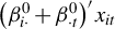 by taking the average of untreated outcomes. Therefore, SCM is essentially based on the model

and treats
$u_{it}^{\dagger }$
 as an unpredictive error. MSE
$_{\hat {\tau } _{it}}$
 based on SCM is at least as large as Var
$(u_{it}^{\dagger }),$
 which is equals to
$4$
 and
$2$
 for DGPs 1 and 2, respectively. The main advantage of our approach is that we are able to utilize the information of covariates. In the Supplementary Material, we compare our approach with SCM for pure factor structures without any covariates and show that both approaches work well. We emphasize that the superior performance of our approach crucially depends on the correct specification of our model. In the Supplementary Material, we design DGPs with grouped factor structure and show that SCM can outperform our method in this special case.
MSE of estimators of TE and ATT
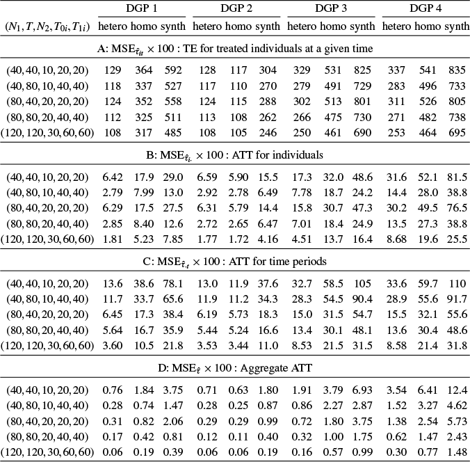
Table 2 Long description
A complex data table titled M S E of estimators of T E and A T T.
Header Structure:
* The top row identifies four Data Generating Processes: D G P 1, D G P 2, D G P 3, and D G P 4.
* Below each D G P are three sub-columns: hetero (heterogeneous model), homo (constant slope model), and synth (synthetic control method).
* The leftmost column lists parameter sets in the format (N sub 1, T, N sub 2, T sub 0 i, T sub 1 i).
Section A: M S E of tau-hat sub i t times 100 (T E for treated individuals at a given time):
* Values range from 105 to 835.
* For (40, 40, 10, 20, 20), D G P 1 hetero is 129, homo is 364, and synth is 592.
* For (120, 120, 30, 60, 60), D G P 4 hetero is 253, homo is 464, and synth is 695.
Section B: M S E of tau-hat sub i dot times 100 (A T T for individuals):
* Values range from 1.72 to 81.5.
* For (40, 40, 10, 20, 20), D G P 1 hetero is 6.42, homo is 17.9, and synth is 29.0.
* For (120, 120, 30, 60, 60), D G P 4 hetero is 8.68, homo is 19.6, and synth is 25.5.
Section C: M S E of tau-hat sub dot t times 100 (A T T for time periods):
* Values range from 3.44 to 110.
* For (40, 40, 10, 20, 20), D G P 1 hetero is 13.6, homo is 38.6, and synth is 78.1.
* For (120, 120, 30, 60, 60), D G P 4 hetero is 8.58, homo is 21.4, and synth is 31.8.
Section D: M S E of tau-hat times 100 (Aggregate A T T):
* Values range from 0.06 to 12.4.
* For (40, 40, 10, 20, 20), D G P 1 hetero is 0.76, homo is 1.84, and synth is 3.75.
* For (120, 120, 30, 60, 60), D G P 4 hetero is 0.30, homo is 0.77, and synth is 1.48.
General Trend: Across all sections and D G P s, the hetero estimator consistently yields the lowest M S E, followed by homo, with synth typically yielding the highest M S E.
Note: hetero refers to the heterogeneous model proposed in this article, homo refers to the model where the slope coefficients are imposed to be constant, and synth refers to SCM (synthetic control method).
Table 3 presents the actual coverage of the 95% CI for the TE,
$ \tau _{it}$
 and ATT,
$\tau _{i\cdot }, \tau _{\cdot t},$
 and
$\tau .$
 The CI of
$\tau _{it}$
 is based on the quantiles of the residuals and the CIs of
$\tau _{i\cdot }, \tau _{\cdot t},$
 and
$\tau $
 are based on our asymptotic normality result in Theorem 4.1. The actual coverages are slightly under-covered when the sample size is small, however they are all close to 95% when the sample size is relatively large. This suggests the validity of our inference procedure.
Empirical coverage of 95% confidence intervals
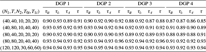
Table 3 Long description
The table is organized into 17 columns. The first column lists input coordinates in the format (N sub 1, T, N sub 2, T sub 0 i, T sub 1 i). The remaining 16 columns are grouped under four main headers: D G P 1, D G P 2, D G P 3, and D G P 4. Each D G P group contains four sub-columns for the parameters tau sub i t, tau sub i dot, tau sub dot t, and tau.
Data rows by input coordinates:
* (40, 40, 10, 20, 20): D G P 1 (0.90, 0.93, 0.89, 0.91); D G P 2 (0.90, 0.92, 0.90, 0.92); D G P 3 (0.88, 0.92, 0.87, 0.88); D G P 4 (0.87, 0.87, 0.86, 0.85).
* (40, 80, 10, 40, 40): D G P 1 (0.93, 0.95, 0.92, 0.95); D G P 2 (0.93, 0.94, 0.92, 0.94); D G P 3 (0.92, 0.93, 0.91, 0.92); D G P 4 (0.91, 0.89, 0.90, 0.89).
* (80, 40, 20, 20, 20): D G P 1 (0.90, 0.92, 0.90, 0.92); D G P 2 (0.90, 0.93, 0.90, 0.95); D G P 3 (0.89, 0.92, 0.89, 0.93); D G P 4 (0.88, 0.89, 0.88, 0.91).
* (80, 80, 20, 40, 40): D G P 1 (0.93, 0.94, 0.93, 0.92); D G P 2 (0.93, 0.94, 0.93, 0.96); D G P 3 (0.92, 0.94, 0.92, 0.96); D G P 4 (0.91, 0.92, 0.92, 0.93).
* (120, 120, 30, 60, 60): D G P 1 (0.94, 0.94, 0.93, 0.95); D G P 2 (0.94, 0.95, 0.94, 0.94); D G P 3 (0.93, 0.94, 0.93, 0.94); D G P 4 (0.93, 0.92, 0.93, 0.94).
In Section S.7.3 of our Supplementary Material, we show that when
$\beta _{\cdot t}$
 is nonstationary, the permutation test proposed in Chernozhukov et al. (Reference Chernozhukov, Wüthrich and Zhu2021) applied to SCM may have severe size distortion. The nonstationarity of
$ \beta _{\cdot t}$
 causes nonstationarity of the error term in SCM, which invalidates many existing inference procedures, such as Chernozhukov et al. (Reference Chernozhukov, Wüthrich and Zhu2021), Masini and Medeiros (Reference Masini and Medeiros2021), and Masini and Medeiros (Reference Masini and Medeiros2022). Our approach estimates all
$\beta _{\cdot t}$
 as unknown parameters, and therefore is immune to this problem.
6 AN EMPIRICAL APPLICATION
In this section, we apply our new method to study the effect of economic liberalization on economic growth, which is an important question in international economics and has received considerable attention. Although it is intuitive to argue that the effect of liberalization should be positive, empirical studies remain challenging and the topic is still being heatedly debated; see, e.g., Sachs et al. (Reference Sachs, Warner, Åslund and Fischer1995), Rodriguez and Rodrik (Reference Rodriguez and Rodrik2000), and Billmeier and Nannicini (Reference Billmeier and Nannicini2013, BN hereafter).
We consider a sample of 60 countries over 30 years (1965–1994), that is,
$N=60$
 and
$T=30$
 . The construction of the sample is mainly based on data availability. The outcome variable
$y_{it}$
 is country i’s economic growth in year
$t.$
 The treatment indicator is whether a country is classified as “open” in year
$t.$
 The treatment variable is constructed by Sachs et al. (Reference Sachs, Warner, Åslund and Fischer1995) and updated by Wacziarg and Welch (Reference Wacziarg and Welch2008). A country at one year is considered “close” if it satisfies certain conditions, such as imposing high tariffs, using large nontariff barriers, or having a socialist economic system, among others. For the detailed criterion for being “close,” see, for example, BN (p. 985). There are many covariates that can potentially explain economic growth (see, e.g., Durlauf, Johnson, and Temple, Reference Durlauf, Johnson and Temple2005, for a comprehensive literature review). Considering the relatively small sample size here, we cannot include many covariates. We choose two important ones: investment share (share of gross capital formation) and consumption share (share of household consumption) out of a country’s GDP measured at current purchasing power parities (PPPs). Investment and consumption are usually the two major components of a country’s GDP. In our sample, the average investment share is about 17% and the average consumption share is about 67%. The economic growth data are constructed from the real GDP per capita data used in BN and the treatment indicator is directly from BN. The data source of investment and consumption share data is the Penn World Table.
There are 25 control countries, meaning that they remained “close” for the whole sample period. Thirty-five countries are treated, meaning that they became open at certain years. We rule out countries that were always open or open for more than 20 years in our sample period.Footnote 6 The summary statistics are reported in Table S.4 in Section S.7 of the Supplementary Material. The list of treated and control countries can be found in Table S.5 in the Supplementary Material. In total, we have 241 treated outcomes in our sample.
Table 4 reports estimates of treatment effects based on various methods. We first consider our hetero model. We find that the estimate of the aggregate ATT is 1.24 with a 95% CI of [0.57, 1.92]. This suggests that being “open” can lead to 1.24% economic growth annually on average. The positive effect is largely consistent with the literature. For example, Sachs et al. (Reference Sachs, Warner, Åslund and Fischer1995) state that “open economies grow, on average, by 2.45 percentage points more than close economies, with a highly statistically significant effect.” Romalis (Reference Romalis2007) concludes that “eliminating existing developed world tariffs would increase developing country growth rates by 0.6 to 1.6 percent per annum.” We also try alternative methods, which are labeled as “simple,” “synth,” and “homo” in Table 4. The “simple” method refers to the regression of
$y_{it}$
 on the binary treatment indicator and two covariates and the coefficient on the treatment indicator is interpreted as a treatment effect. For the aggregate ATT, TWFEs are included. The “synth” method refers to SCM where we use the average of pre-treatment covariates and all pre-treatment outcomes as predictors. The “homo” method refers to the same model as “hetero” except that the slope coefficient
$\beta _{i\cdot }^{0}+\beta _{\cdot t}^{0}$
 is imposed to be constant. The estimates based on the three alternative methods are all positive, though the magnitudes (0.62 [simple], 1.05 [synth], and 0.22 [homo]) differ. This suggests the robustness of the “positive effects.”
Treatment effects
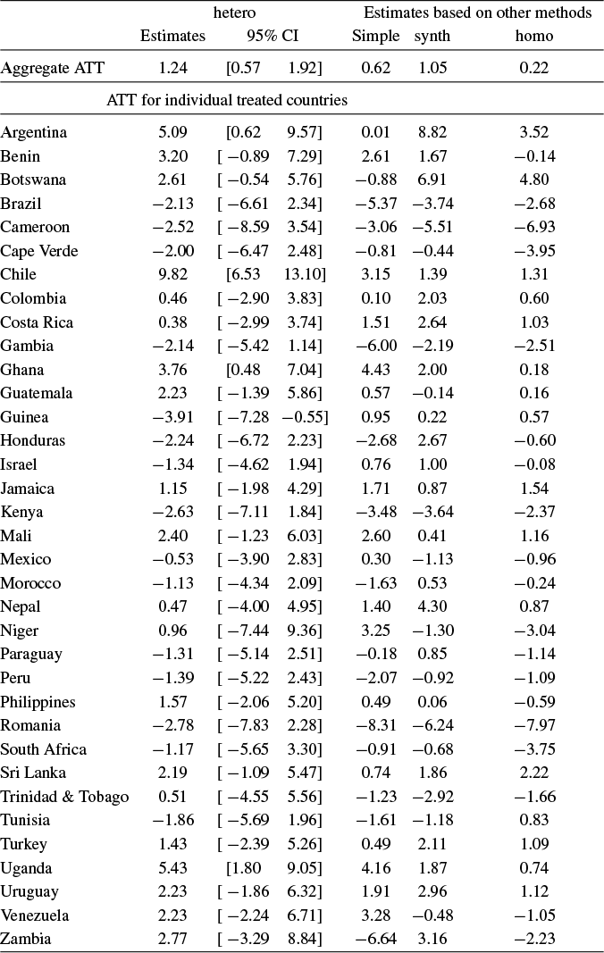
Table 4 Long description
The table is divided into two main sections: Aggregate A T T and A T T for individual treated countries.
* Aggregate A T T: hetero estimate is 1.24 with a 95% C I of [0.57, 1.92]. Other methods show Simple at 0.62, synth at 1.05, and homo at 0.22.
Individual country data for the hetero method and other estimates:
* Argentina: hetero 5.09 [0.62, 9.57], Simple 0.01, synth 8.82, homo 3.52.
* Benin: hetero 3.20 [-0.89, 7.29], Simple 2.61, synth 1.67, homo -0.14.
* Botswana: hetero 2.61 [-0.54, 5.76], Simple -0.88, synth 6.91, homo 4.80.
* Brazil: hetero -2.13 [-6.61, 2.34], Simple -5.37, synth -3.74, homo -2.68.
* Cameroon: hetero -2.52 [-8.59, 3.54], Simple -3.06, synth -5.51, homo -6.93.
* Cape Verde: hetero -2.00 [-6.47, 2.48], Simple -0.81, synth -0.44, homo -3.95.
* Chile: hetero 9.82 [6.53, 13.10], Simple 3.15, synth 1.39, homo 1.31.
* Colombia: hetero 0.46 [-2.90, 3.83], Simple 0.10, synth 2.03, homo 0.60.
* Costa Rica: hetero 0.38 [-2.99, 3.74], Simple 1.51, synth 2.64, homo 1.03.
* Gambia: hetero -2.14 [-5.42, 1.14], Simple -6.00, synth -2.19, homo -2.51.
* Ghana: hetero 3.76 [0.48, 7.04], Simple 4.43, synth 2.00, homo 0.18.
* Guatemala: hetero 2.23 [-1.39, 5.86], Simple 0.57, synth -0.14, homo 0.16.
* Guinea: hetero -3.91 [-7.28, -0.55], Simple 0.95, synth 0.22, homo 0.57.
* Honduras: hetero -2.24 [-6.72, 2.23], Simple -2.68, synth 2.67, homo -0.60.
* Israel: hetero -1.34 [-4.62, 1.94], Simple 0.76, synth 1.00, homo -0.08.
* Jamaica: hetero 1.15 [-1.98, 4.29], Simple 1.71, synth 0.87, homo 1.54.
* Kenya: hetero -2.63 [-7.11, 1.84], Simple -3.48, synth -3.64, homo -2.37.
* Mali: hetero 2.40 [-1.23, 6.03], Simple 2.60, synth 0.41, homo 1.16.
* Mexico: hetero -0.53 [-3.90, 2.83], Simple 0.30, synth -1.13, homo -0.96.
* Morocco: hetero -1.13 [-4.34, 2.09], Simple -1.63, synth 0.53, homo -0.24.
* Nepal: hetero 0.47 [-4.00, 4.95], Simple 1.40, synth 4.30, homo 0.87.
* Niger: hetero 0.96 [-7.44, 9.36], Simple 3.25, synth -1.30, homo -3.04.
* Paraguay: hetero -1.31 [-5.14, 2.51], Simple -0.18, synth 0.85, homo -1.14.
* Peru: hetero -1.39 [-5.22, 2.43], Simple -2.07, synth -0.92, homo -1.09.
* Philippines: hetero 1.57 [-2.06, 5.20], Simple 0.49, synth 0.06, homo -0.59.
* Romania: hetero -2.78 [-7.83, 2.28], Simple -8.31, synth -6.24, homo -7.97.
* South Africa: hetero -1.17 [-5.65, 3.30], Simple -0.91, synth -0.68, homo -3.75.
* Sri Lanka: hetero 2.19 [-1.09, 5.47], Simple 0.74, synth 1.86, homo 2.22.
* Trinidad and Tobago: hetero 0.51 [-4.55, 5.56], Simple -1.23, synth -2.92, homo -1.66.
* Tunisia: hetero -1.86 [-5.69, 1.96], Simple -1.61, synth -1.18, homo 0.83.
* Turkey: hetero 1.43 [-2.39, 5.26], Simple 0.49, synth 2.11, homo 1.09.
* Uganda: hetero 5.43 [1.80, 9.05], Simple 4.16, synth 1.87, homo 0.74.
* Uruguay: hetero 2.23 [-1.86, 6.32], Simple 1.91, synth 2.96, homo 1.12.
* Venezuela: hetero 2.23 [-2.24, 6.71], Simple 3.28, synth -0.48, homo -1.05.
* Zambia: hetero 2.77 [-3.29, 8.84], Simple -6.64, synth 3.16, homo -2.23.
Note: “hetero” refers to the heterogeneous model proposed in this paper, “simple” refers to regressing the growth on the treatment indicator and covariates, “synth” refers to SCM (synthetic control method), and “homo” refers to the model where the slope coefficients are imposed to be constant. The CI is based on the pre-whitening HAC estimator of the variance term.
Estimates of
$ \beta _{i\cdot }$
 and
$ \beta _{\cdot t}$
 (demeaned).

Figure 1 Long description
Panel A is a histogram of beta sub i dot estimates for investment share. The x-axis ranges from minus 1 to 3, and the y-axis shows the number of observations from 0 to 25. The distribution is centered near minus 0.25 with a S T D of 0.637. Panel B is a histogram for consumption share with an x-axis from minus 0.2 to 0.4 and a y-axis from 0 to 20. The distribution is centered near 0 with a S T D of 0.095. Panel C is a line graph of beta sub dot t estimates for investment share from 1965 to 1995. The y-axis ranges from minus 0.4 to 0.4. The blue dashed line with circular markers shows high volatility with a S T D of 0.174. Panel D is a line graph for consumption share over the same period. The y-axis ranges from minus 0.1 to 0.1. The trend shows a peak around 1970 followed by a decline and fluctuations with a S T D of 0.048.
Table 4 also presents the ATT for each individual treated country. We find that 20 treated countries have a positive ATT, while 15 treated countries have a negative ATT. Table 4 also reports their 95% CIs. Note that in our sample, the time period is quite short, therefore, the CIs are usually wide. Only five countries’ ATT are statistically significant at the 5% level (Argentina, Chile, Ghana, Guinea, and Uganda). Among the five countries, only one country (Guinea) has a negative effect. Table 4 also reports the estimates based on alternative methods. Although the exact estimates are different, there are some commonalities in the results. For example, if we compare the results between our hetero model and the synthetic control, 26 out of 35 ATT estimates share the same sign.
One important feature of our model is that we allow a general form of heterogeneity, which is supported by our empirical results. Figure 1 shows the histogram of the demeaned estimates of
$\beta _{i\cdot }$
 for investment share and consumption share. Figure 1 also plots the demeaned estimates of
$\beta _{\cdot t}$
 for those two variables over time. The detailed estimates are reported in Tables S.5 and S.6 in the Supplementary Material. We observe a wide range of variations in the estimates, in particular the slope coefficient for investment share.Footnote
7
The average estimates of the slope coefficients of investment share and consumption share are 0.381 and
$-$
 0.026, respectively. This shows that investment share has a large positive effect on a country’s economic growth. We also find one unobservable factor, which suggests one common factor or shock that drives all countries’ growth.
In sum, we find that the aggregate ATT of liberalization on countries’ economic growth is positive and statistically significant. On average, “being open” leads to 1.24% economic growth annually. The ATT for individual countries is quite heterogeneous, though most of them are positive. We also find that investment share has a large positive effect on economic growth.
7 CONCLUSION
In this article, we consider the heterogeneous panel data models with IFEs where the slope coefficients of the covariates exhibit unobserved heterogeneity over both the individual and time dimensions. We propose a two-step procedure to estimate the parameters and study the asymptotic properties of the estimators. We apply the proposed model to study the consistent estimation of the average of heterogeneous treatment effects on the treated. As an empirical illustration, we investigate the effect of economic liberalization on economic growth and find a positive and significant aggregate ATT.
Our approach is based on a flexible outcome model with covariates and factor structures and can be thought of as an alternative to the popular SCM for estimating treatment effects. There are two main advantages of our approach. First, our estimator exploits the information of covariates and is typically more efficient than SCM if our model is correctly specified. Second, as emphasized above, some existing inference procedures such as that of Chernozhukov et al. (Reference Chernozhukov, Wüthrich and Zhu2021), Masini and Medeiros (Reference Masini and Medeiros2021), and Masini and Medeiros (Reference Masini and Medeiros2022) are typically invalid when
$\{\beta _{\cdot t}^0\} $
 exhibits some nonstationary behavior. Our estimator treats
$\{\beta _{\cdot t}^0\}$
 as unknown parameters to estimate, and thus does not suffer from this issue.
There are several interesting topics for further research. First, although we allow nonstationary
$\{\beta _{\cdot t}\}$
 , we still impose stationarity on covariates and factors. It is helpful to relax those assumptions. Second, a fruitful direction of future research is to augment SCM with our outcome-based model, as in Ben-Michael, Feller, and Rothstein (Reference Ben-Michael, Feller and Rothstein2021). Third, we do not consider unbalanced panels in the current study. For unbalanced panels, we propose an algorithm to estimate the model parameters in Section S.5 of the Supplementary Material without a formal justification. We are exploring these topics in ongoing work.
This appendix establishes the main results of the article by drawing on several technical lemmas proved in Sections S.1.3, S.2.4, S.3, and S.4 of the Supplementary Material. We use
$ O_{P}(\cdot )$
 and
$o_{P}(\cdot )$
 to denote the usual big O and small o in probability, respectively. For a random matrix A that is typically high-dimensional, we write
$A=O_{\mathrm {sp},P}(a_{NT})$
 and
$ A=o_{\mathrm {sp},P}(a_{NT})$
 to indicate
$\Vert A\Vert _{\mathrm {sp} }=O_{P}(a_{NT})$
 and
$\Vert A\Vert _{\mathrm {sp}}=o_{P}(a_{NT})$
 , respectively. For a matrix
$A_{m\times n}$
 , denote the maximum absolute column-sum norm (
$\ell _{1}$
 -norm) and the maximum absolute row-sum norm (
$ \ell _{\infty }$
 -norm) as
$\Vert A\Vert _{1}\equiv \max _{1\leq j\leq n}\sum _{i=1}^{m}|a_{ij}|$
 and
$\Vert A\Vert _{\infty }\equiv \max _{1\leq i\leq m}\sum _{j=1}^{n}|a_{ij}|.$
 When A is an m-vector (
$n=1$
 ), we have that
$\Vert A\Vert _{\infty }$
 represents the maximum of absolute value of its elements. We also define
$\Vert A\Vert _{2,\infty }=\max _{1\leq i\leq m}\Vert A_{i,\cdot }\Vert =\max _{1\leq i\leq m}\sqrt {\sum _{j=1}^{n}a_{ij}^{2} },$
 where
$A_{i,\cdot }$
 denotes the ith row of A. The following inequalities will be used frequently:

where x is a conformable vector and B is a matrix.
A PROOFS OF THE MAIN RESULTS
A.1 Asymptotic Analyses for Section 3
To prove Theorem 3.1, we first introduce a lemma whose proof is similar to that of Lemma A.1 of Miao et al. (Reference Miao, Phillips and Su2023).
Lemma A.1.
(i) For any
$T\times N$
 matrix
$\Delta $
 ,
$||\Theta ^{0}+ \mathbb {M}_{F^{0}}\Delta \mathbb {M}_{\Lambda ^{0}}||_{\ast }=||\Theta ^{0}||_{\ast }+||\mathbb {M}_{F^{0}}\Delta \mathbb {M}_{\Lambda ^{0}}||_{\ast } $
 .
(ii) For any conformable matrices A and B,
$|\mathrm {tr}(A^{\prime }B)|\leq ||A||_{sp}||B||_{\ast }$
 .
(iii) rank
$(\Delta -\mathbb {M}_{F^{0}}\Delta \mathbb {M}_{\Lambda ^{0}})\leq 2R^{0}$
 .
(iv) For a matrix A with rank
$(A)=r$
 ,
$||A||_{\ast }\leq \sqrt {r}||A||.$

Proof of Theorem 3.1
Let
$\hat {\Delta } _{\Theta }=\hat {\Theta }_{o}-\Theta ^{0}$
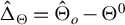 and
$\hat {\delta }_{\theta }=$
 vec
$(\hat {\Delta }_{\Theta }).$
 Comparing the values of
$\mathcal {\tilde {L}} _{NT}(\Theta )+\gamma _{NT}\left \vert \left \vert \Theta \right \vert \right \vert _{\text {*}}/\sqrt {NT}$
 at
$\hat {\Theta }_{o}$
 and
$\Theta ^{0},$
 we have

where the second inequality holds by the triangle inequality and the last equality follows by Lemma A.1(i). Note that
$\hat {\delta }_{\theta }^{^{\prime }}\mathbb {M}_{x}U=$
 tr
$[\hat {\Delta }_{\Theta }^{\prime }\mathrm {\ mat}(\mathbb {M}_{x}U)].$
 By Lemma A.1(ii), Assumption 1, and the triangle inequality, the following inequality holds w.p.a.1:

Combining inequalities (A.1) and (A.2), we have that

Inequality (A.3) implies that
$\hat {\Delta }_{\Theta }\in \mathbb {C} _{NT}$
 , where
$\mathbb {C}_{NT}$
 is defined in Assumption 2. By Assumption 2, inequality (A.3), and Lemma A.1 (iii) and (iv), there exists a positive constant
$\mu $
 such that

It follows that
$\frac {||\hat {\Delta }_{\Theta }||}{\sqrt {NT}}\leq \frac {3 \sqrt {2R^{0}}}{\mu }\gamma _{NT}$
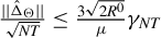 .
Proof of Theorem 3.2
(i) The proof follows from that of Theorem 3.2 in Hong et al. (Reference Hong, Su and Jiang2023) and thus omitted.
(ii) Let
$S_{F}=T^{-1}F^{0\prime }F^{0}, S_{\Lambda }=N^{-1}\Lambda ^{0\prime }\Lambda ^{0},$
 and
$\tilde {H}=S_{F}^{-1/2}v,$
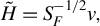 where v is the
$ R^{0}\times R^{0}$
 matrix whose columns are the eigenvectors of
$ S_{F}^{1/2}S_{\Lambda }S_{F}^{1/2}.$
 Conditional on
$\hat {R}=R^{0},$
 we can bound
$T^{-1/2}\left \Vert \hat {F}_{o}-F^{0}\tilde {H}\right \Vert .$
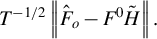 Specifically, we can follow Miao et al. (Reference Miao, Phillips and Su2023) and apply the Davis–Kahan sin
$ \left (\Theta \right ) $
 theorem (e.g., Yu, Wang, and Samworth, Reference Yu, Wang and Samworth2015) to obtain the following bound:
$T^{-1/2}\left \Vert \hat {F}_{o}-F^{0}\tilde {H}\right \Vert =O_{P}\left (\gamma _{NT}\right ) $
 under Assumptions 1–3, which implies that
$\Vert \mathbb {M}_{\hat {F}_{o}}-\mathbb {M} _{F^{0}}\Vert =O_{P}\left (\gamma _{NT}\right ) .$

(iii) Analogous arguments of the last point show that
$N^{-1/2}\left \Vert \hat { \Lambda }_{o}-\Lambda ^{0}(\tilde {H}^{-1})^{\prime }\right \Vert =O_{P}\left (\gamma _{NT}\right ) $
 and
$\Vert \mathbb {M}_{\hat {\Lambda }_{o}}-\mathbb {M} _{\Lambda ^{0}}\Vert =O_{P}\left (\gamma _{NT}\right ) $
 .
To prove Theorem 3.3, we introduce Lemmas A.2 and A.3 and some notations. Let

where
$\tilde {Q}_{kl}=X^{(k)\prime }(\mathbb {M}_{\Lambda ^{0}}\otimes \mathbb {M}_{F^{0}})X^{(l)}$
 for
$k,l=1,2$
 . In Section S.1 of the Supplementary Material, we show that
$\tilde {Q}$
 is invertible w.p.a.1 under Assumption 4. Define the inverse of
$\tilde {Q}$
 , an
$ (N-1+T)K\times (N-1+T)K$
 matrix, as

where
$\mathbb {\tilde {Q}}_{kl}$
 has the same size as
$\tilde {Q}_{kl}$
 .
Lemma A.2. Let
$\mathbf {q}_{a}^{(1)}= \begin {pmatrix} \dot {q}_{1}^{\prime } & \dot {q}_{2}^{\prime } & \cdots & \dot {q} _{N-1}^{\prime } \end {pmatrix} ^{\prime }$
 and
$\mathbf {q}_{a}^{(2)}= \begin {pmatrix} \ddot {q}_{1}^{\prime } & \ddot {q}_{2}^{\prime } & \cdots & \ddot {q} _{T}^{\prime } \end {pmatrix} ^{\prime }$
 . Suppose Assumptions 3–5 hold. Then we have:
(i)
$||\sqrt {T}\mathbb {\tilde {Q}}_{12}\mathbf {q}^{(2)}||_{\infty }=O_{P}[(\log ^{2}N+\log ^{2}T)/\sqrt {N}]$
 ;
(ii)
$||\sqrt {N}\mathbb {\tilde {Q}}_{21}\mathbf {q}^{(1)}||_{\infty }=O_{P}[(\log ^{2}N+\log ^{2}T)/\sqrt {T}]$
 ;
(iii)
$||\sqrt {T}\mathbb {\tilde {Q}}_{11}\mathbf {q}^{(1)}-\dot {\mathbf {S}} _{(1)}^{-1}\mathbf {q}_{a}^{(1)}/\sqrt {T}||_{\infty }=O_{P}[(\log ^{2}N+\log ^{2}T)/\sqrt {T}]$
 ;
(iv)
$||\sqrt {N}\mathbb {\tilde {Q}}_{22}\mathbf {q}^{(2)}-\ddot {\mathbf {S}} _{(2)}^{-1}\mathbf {q}_{a}^{(2)}/\sqrt {N}||_{\infty }=O_{P}[(\log ^{2}N+\log ^{2}T)/\sqrt {N}]$
 .
Lemma A.3. Suppose Assumptions 3–5 hold. Then we have:
(i)
$\sqrt {T}(\iota _{N-1}^{\prime }\otimes \mathbb {I}_{K})\tilde {\mathbb {Q}} _{11}\mathbf {q}^{(1)}=\dot {\mathbf {s}}_{N\cdot }^{-1}\dot {q}_{N}/\sqrt {T} +O_{P}[(\log ^{2}N+\log ^{2}T)/\sqrt {N}]$
 ;
(ii)
$\sqrt {T}(\iota _{N-1}^{\prime }\otimes \mathbb {I}_{K})\mathbb {\tilde {Q} }_{12}\mathbf {q}^{(2)}=O_{P}[(\log ^{2}N+\log ^{2}T)/\sqrt {N}]$
 .
The proofs of Lemmas A.1–A.3 are provided in Section S.1.3 of the Supplementary Material.
Proof of Theorem 3.3
Step 1. Obtain explicit expression of
$\boldsymbol {\check {B}-\dot {B}}$
 .
Recall the definition of
$\check {B}$
 as in (3.1), we have

As both
$X^{(1,2)\prime }(\mathbb {M}_{\Lambda ^{0}}\otimes \mathbb {M} _{F^{0}})X^{(1,2)}$
 and
$X^{(1,2)\prime }(\mathbb {M}_{\Lambda ^{0}}\otimes \mathbb {M}_{F^{0}})U$
 are high-dimensional objects, it is essential to carefully analyze their properties. After proper normalization, we have

where
$\mathbb {L}_{NT}\equiv {\mathrm {blkdiag}}(\sqrt {T}\mathbb {I}_{K(N-1)},\sqrt {N} \mathbb {I}_{KT})$
 .
Step 2. Verify that
$\max _{1\leq i\leq N-1}||\sqrt {T}(\check {\beta }_{i\cdot }-\dot {\beta }_{i\cdot })-\dot {\mathbf {s}}_{i\cdot }^{-1}\dot {q}_{i}/\sqrt {T}||=o_{P}(1)$
 and
$\max _{1\leq t\leq T}||\sqrt {N}(\check {\beta }_{\cdot t}-\dot {\beta }_{\cdot t})-\ddot {\mathbf {s}}_{\cdot t}^{-1}\ddot {q}_{t}/\sqrt {N}||=o_{P}(1).$

Recall that
$\dot {\mathbf {S}}_{(1)}\equiv \begin {pmatrix} \dot {\mathbf {s}}_{1\cdot } & & \\ & \ddots & \\ & & \dot {\mathbf {s}}_{N-1\cdot } \end {pmatrix} $
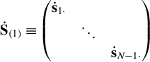 ,
$\dot {\mathbf {S}}_{(2)}\equiv \begin {pmatrix} \ddot {\mathbf {s}}_{\cdot 1} & & \\ & \ddots & \\ & & \ddot {\mathbf {s}}_{\cdot T} \end {pmatrix} $
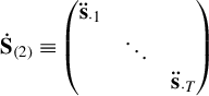 ,
$\mathbf {q}_{a}^{(1)}\equiv \begin {pmatrix} \dot {q}_{1} \\ \vdots \\ \dot {q}_{N-1} \end {pmatrix} $
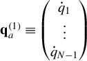 ,
$\mathbf {q}_{a}^{(2)}\equiv \begin {pmatrix} \ddot {q}_{1} \\ \vdots \\ \ddot {q}_{T} \end {pmatrix} $
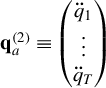 ,
$\dot {\mathbf {S}}_{(1)}^{-1}\mathbf {q}_{a}^{(1)}=\Big(\sum _{t=1}^{T}u_{1t}\dot {x}_{1t}^{\prime }(\sum _{t=1}^{T}\dot {x}_{1t}\dot {x} _{1t}^{\prime })^{-1},\ldots ,\sum _{t=1}^{T}u_{N-1,t}\dot {x}_{N-1,t}^{\prime }$
 $(\sum _{t=1}^{T}\dot {x}_{N-1,t}\dot {x}_{N-1,t}^{\prime })^{-1}\Big) ^{\prime }$
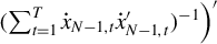 and
$\ddot {\mathbf {S}}_{(2)}^{-1}\mathbf {q}_{a}^{(2)}=\Big(\sum _{i=1}^{N}u_{i1}\dot {x}_{i1}^{\prime }(\sum _{i=1}^{N}\dot {x}_{i1}\dot {x} _{i1}^{\prime })^{-1},\ldots , \sum _{i=1}^{N}u_{iT}\dot {x}_{iT}^{\prime }(\sum _{i=1}^{N}\dot {x}_{iT}\dot {x}_{iT}^{\prime })^{-1}\big) ^{\prime }$
 .
Verifying
$\max _{1 \leq i \leq N-1}||\sqrt {T}(\check {\beta }_{i\cdot }-\dot { \beta }_{i\cdot })-\dot {\mathbf {s}}_{i\cdot }^{-1}\dot {q}_{i}/\sqrt {T}||=o_P(1)$
 , and
$\max _{1 \leq t \leq T}||\sqrt {N}(\check {\beta }_{\cdot t}-\dot {\beta } _{\cdot t})-\ddot {\mathbf {s}}_{\cdot t}^{-1}\ddot {q}_{t}/\sqrt {N}||=o_P(1) $
 is equivalent to showing

This result is a direct consequence of Lemma A.2: (1)
$||\sqrt {T} \mathbb {\tilde {Q}}_{12}\mathbf {q}^{(2)}||_\infty =o_P(1)$
 , (2)
$||\sqrt {N} \mathbb {\tilde {Q}}_{21}\mathbf {q}^{(1)}||_\infty =o_P(1)$
 , (3)
$||\sqrt {T} \mathbb {\tilde {Q}}_{11}\mathbf {q}^{(1)} -\dot {\mathbf {S}}_{(1)}^{-1} \mathbf { q}_a^{(1)}/\sqrt {T}||_\infty =o_P(1)$
 , and (4)
$||\sqrt {N}\mathbb {\tilde {Q}} _{22}\mathbf {q}^{(2)} -\ddot {\mathbf {S}}_{(2)}^{-1} \mathbf {q}_a^{(2)}/\sqrt { N}||_\infty =o_P(1)$
 .
Step 3. Verify
$\boldsymbol {\sqrt {T}(\check {\beta }_{N\cdot }-\dot {\beta } _{N\cdot })=\dot {\mathbf {s}}_{N\cdot }^{-1}\dot {q}_{N}/\sqrt {T}+o_P(1).}$

It remains to study
$\check {\beta }_{N\cdot }-\dot {\beta }_{N\cdot },$
 where
$ \dot {\beta }_{N\cdot }=-\sum _{i=1}^{N-1}\dot {\beta }_{i\cdot }=-(\iota _{N-1}^{\prime }\otimes \mathbb {I}_{K})\dot {B}^{(1)}$
 and
$\check {\beta } _{N\cdot }=-\sum _{i=1}^{N-1}\check {\beta }_{i\cdot }=-(\iota _{N-1}^{\prime }\otimes \mathbb {I}_{K})\check {B}^{\left (1\right ) }$
 . Then we have

where
$-\sqrt {T}(\iota _{N-1}^{\prime }\otimes \mathbb {I}_{K})\mathbb {\tilde { Q}}_{11}\mathbf {q}^{(1)}=-\dot {\mathbf {s}}_{N\cdot }^{-1}\dot {q}_{N}/\sqrt {T} +O_{P}(\log ^{2}N/\sqrt {N})$
 and
$\sqrt {T}(\iota _{N-1}^{\prime }\otimes \mathbb {I}_{K})\mathbb {\tilde {Q}}_{12}\mathbf {q}^{(2)}=O_{P}(\log N/\sqrt {N} ) $
 , by Lemma A.3. It follows that
$\sqrt {T}(\check {\beta } _{N\cdot }-\dot {\beta }_{N\cdot })=-\dot {\mathbf {s}}_{N\cdot }^{-1}\dot {q} _{N}/\sqrt {T}+O_{P}(\log ^{2}N/\sqrt {N})$
 .
To prove Theorem 3.4, we introduce Lemmas A.4 and A.5 and some notations. Let
$\Lambda \in \mathbb {R}^{N\times R^{0}}$
 and
$F\in \mathbb {R}^{T\times R^{0}}$
 . Define

Next, define the projected score vectors

so that the vectors
$\mathbf {q}^{(1)}$
 and
$\mathbf {q}^{(2)}$
 from the previous section are obtained by evaluating at the true factors and loadings
$(\Lambda ^{0},F^{0})$
 . Further, define

which equal zero when
$(\Lambda ,F)=(\Lambda ^{0},F^{0})$
 .
Lemma A.4. Under the conditions for Theorem 3.4, we have
(i)
$\tilde {Q}(\hat {\Lambda }^{(2)},\hat {F}^{(2)})$
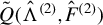 is asymptotically non-singular, with expansion

where
$||\mathbb {L}_{NT}\tilde {\mathbb {Q}}\mathbb {L}_{NT}||_{sp}=O_{P}(1)$
 , and
$||\mathbb {L}_{NT}\tilde {\mathbb {Q}}\sum _{j=1}^{\infty }[(\tilde {Q}- \tilde {Q}(\hat {\Lambda }^{(2)},\hat {F}^{(2)}))\tilde {\mathbb {Q}}]^{j}\mathbb {L }_{NT}||_{sp}=o_{P}(1)$
 ;
(ii)
$||\mathbb {L}_{NT}^{-1}(\tilde {Q}(\hat {\Lambda }^{(2)},\hat {F}^{(2)})- \tilde {Q})\mathbb {L}_{NT}^{-1}||_{2,\infty }=O_{P}(\delta _{NT}^{-2}\log (NT)),$
 and
$||\mathbb {L}_{NT}^{-1}(\tilde {Q}(\hat {\Lambda }^{(2)},\hat {F} ^{(2)})-\tilde {Q})\mathbb {L}_{NT}^{-1}||_{sp} =O_{P}(\sqrt {N+T}\delta _{NT}^{-2}\log (NT))$
 ;
(iii)
$||\mathbf {q}_{\theta }^{(1)}(\hat {\Lambda }^{(2)},\hat {F} ^{(2)})||=o_{P}(\sqrt {T})$
 , and
$||\mathbf {q}_{\theta }^{(2)}(\hat {\Lambda } ^{(2)},\hat {F}^{(2)})||=o_{P}(\sqrt {N});$

(iv)
$||\mathbb {L}_{NT}^{-1}\mathbf {q}(\hat {\Lambda }^{(2)},\hat {F} ^{(2)})||=O_{P}(\sqrt {N+T}).$

Lemma A.5. Under the conditions for Theorem 3.4, we have
(i)
$\left \Vert \mathbb {L}_{NT}\tilde {\mathbb {Q}}(\mathbf {q}(\hat {\Lambda } ^{(2)},\hat {F}^{(2)})-\mathbf {q})\right \Vert _{\infty }=o_{P}(1),$
 and
$|| \mathbb {L}_{NT}\tilde {\mathbb {Q}}(\mathbf {q}(\hat {\Lambda }^{(2)},\hat {F} ^{(2)})-\mathbf {q})||=O_{P}(\sqrt {N+T}\delta _{NT}^{-1}\log ^{2}(NT))$
 ;
(ii)
$\left \Vert \mathbb {L}_{NT}\tilde {\mathbb {Q}}\mathbf {q}_{\theta }(\hat { \Lambda }^{(2)},\hat {F}^{(2)})\right \Vert =o_{P}(1)$
 ;
(iii)
$||\mathbb {L}_{NT}^{-1}\tilde {Q}^{(\infty )}\mathbb {L} _{NT}^{-1}||_{2,\infty }=O_{P}(\log (NT)/\sqrt {NT})$
 and
$||\mathbb {L}_{NT} \tilde {\mathbb {Q}}\tilde {Q}^{(2,rem)}\tilde {\mathbb {Q}}\mathbb {L} _{NT}||_{sp}=O_{P}(\log ^{2}(NT)\delta _{NT}^{-2})$
 ;
(iv)
$\left \Vert \mathbb {L}_{NT}\tilde {\mathbb {Q}}\mathbb {L}_{NT}-{\mathrm {blkdiag}}(\dot {\mathbf {S}}_{(1)}^{-1},\ddot {\mathbf {S}}_{(2)}^{-1})\right \Vert _{2,\infty }=O_{P}(\delta _{NT}^{-1}\log (NT)),$

where expressions of
$\tilde {Q}^{(\infty )}$
 and
$\tilde {Q} ^{(2,rem)}$
 are provided in the proof and
$\tilde {Q}-\tilde {Q}(\hat {\Lambda } ^{(2)},\hat {F}^{(2)})=\tilde {Q}^{(\infty )}+\tilde {Q}^{(2,rem)}$
 .
The proofs of the above two lemmas are given in Section S.2.4 of the Supplementary Material.
Proof of Theorem 3.4
We show that
$\hat {B}_2$
 is asymptotically equivalent to the infeasible estimator, that is,
$||\mathbb { L}_{NT}(\hat {B}_2-\check {B})||_{\infty }=o_P(1)$
 . Then Theorem 3.3 leads to the desired result.
Recall that
$\hat {B}_{2}-\dot {B}=\tilde {Q}(\hat {\Lambda }^{(2)},\hat {F} ^{(2)})^{-1}\left [ \mathbf {q}(\hat {\Lambda }^{(2)},\hat {F}^{(2)})+\mathbf {q} _{\theta }(\hat {\Lambda }^{(2)},\hat {F}^{(2)})\right ] $
 . By Lemma A.4 (i), we have

where
$A_{1}\equiv \mathbb {L}_{NT}\tilde {\mathbb {Q}}\mathbf {q}(\hat {\Lambda } ^{(2)},\hat {F}^{(2)})$
 ,
$A_{2}\equiv \mathbb {L}_{NT}\tilde {\mathbb {Q}} \mathbf {q}_{\theta }(\hat {\Lambda }^{(2)},\hat {F}^{(2)})$
 ,
$A_{3}\equiv \mathbb {L}_{NT}\tilde {\mathbb {Q}}[\tilde {Q}-\tilde {Q}(\hat {\Lambda }^{(2)}, \hat {F}^{(2)})]\tilde {\mathbb {Q}}\mathbb {L}_{NT}\delta \mathbf {q}$
 , and
$ \delta \mathbf {q}\equiv \sum _{j=0}^{\infty }(\mathbb {L}_{NT}^{-1}(\tilde {Q}-\tilde {Q}(\hat {\Lambda }^{(2)},\hat {F}^{(2)})\tilde {\mathbb {Q}} \mathbb {L}_{NT} ) ^{j}\mathbb {L}_{NT}^{-1}[ \mathbf {q}(\hat {\Lambda }^{(2)},\hat {F}^{(2)})+\mathbf {q}_{\theta }(\hat {\Lambda }^{(2)},\hat {F} ^{(2)}) ] .$
 It suffices to study
$A_{1}$
 ,
$A_{2}$
 , and
$A_{3}$
 :
1.
$||A_{1}-\mathbb {L}_{NT}\tilde {\mathbb {Q}}\mathbf {q} ||_{\infty }=o_{P}(1)$
 . This result is implied by Lemma A.5(i).
2.
$||A_{2}||_{\infty }=o_{P}(1)$
 . This is implied by Lemma A.5(ii).
3. Finally, we show
$||A_{3}||_{\infty }=o_{P}(1)$
 below.
By Lemma A.4, we have that
$||\mathbb {L}_{NT}^{-1}(\mathbf {q}(\hat { \Lambda }^{(2)},\hat {F}^{(2)})+\mathbf {q}_{\theta }(\hat {\Lambda }^{(2)},\hat {F }^{(2)}))||=O_{P}(\sqrt {N+T})$
 . By the fact that

we have
$||\delta \mathbf {q}||=O_{P}(\sqrt {N+T})$
 . By the identity that
$ \tilde {Q}(\hat {\Lambda }^{(2)},\hat {F}^{(2)})-\tilde {Q}=\tilde {Q}^{(\infty )}+ \tilde {Q}^{(2,rem)}$
 as in Lemma A.5(iii), we have

The spectrum norm bound of
$\tilde {Q}^{(2,rem)}$
 in Lemma A.5(iii) further implies
$||\mathbb {L}_{NT}\tilde {\mathbb {Q}}\tilde {Q}^{(2,rem)} \tilde {\mathbb {Q}}\mathbb {L}_{NT}\delta \mathbf {q}||=O_{P}(\sqrt {N+T}\delta _{NT}^{-2}\log ^{2}(NT))=o_{P}(1)$
 . For
$||\mathbb {L}_{NT}\tilde {\mathbb {Q}} \tilde {Q}^{(\infty )}\tilde {\mathbb {Q}}\mathbb {L}_{NT}\delta \mathbf {q}$
 , we have

To bound
$A_{3,1}$
 and
$A_{3,2},$
 we first bound
$\left \Vert \mathbb {L} _{NT}^{-1}\tilde {Q}^{(\infty )}\tilde {\mathbb {Q}}\mathbb {L}_{NT}\delta \mathbf {q}\right \Vert $
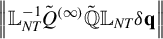 and
$\left \Vert \mathbb {L}_{NT}^{-1}\tilde {Q} ^{(\infty )}\tilde {\mathbb {Q}}\mathbb {L}_{NT}\delta \mathbf {q}\right \Vert _{\infty }$
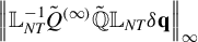 . By Lemma A.5(iii), we have

and
$||\mathbb {L}_{NT}^{-1}\tilde {Q}^{(\infty )}\tilde {\mathbb {Q}}\mathbb {L} _{NT}\delta \mathbf {q}||=O_{P}(\sqrt {N+T}\delta _{NT}^{-1}\log (NT))$
 . It follows that
$A_{3,1}=O_{P}(\sqrt {N+T}\delta _{NT}^{-2}\log ^{2}(NT))=o_{P}(1)$
 where we also use Lemma A.5(iv). Similarly,
$ A_{3,2}=O_{P}(\delta _{NT}^{-1}\log (NT))=o_{P}(1)$
 as
$||{\mathrm {blkdiag}}(\dot { \mathbf {S}}_{(1)}^{-1},\ddot {\mathbf {S}}_{(2)}^{-1})||_{\infty } =O_{P}(1)$
 and
$\left \Vert \mathbb {L}_{NT}^{-1}\tilde {Q}^{(\infty )}\tilde {\mathbb {Q}} \mathbb {L}_{NT}\delta \mathbf {q}\right \Vert _{\infty }=O_{P}(\delta _{NT}^{-1}\log (NT))$
 . Then
$||A_{3}||_{\infty }=o_{P}(1)$
 .
Proof of Theorem 3.5
(i) Note that
$\sqrt {T}(\hat {\beta }_{i\cdot }-\beta _{i\cdot }^{0})=-\sqrt { \frac {T}{N}}\frac {1}{\sqrt {N}}\sum _{j=1}^{N}\beta _{j\cdot }^{0}+ (\frac {1}{T} \mathbf {x}_{i\cdot }^{\prime }\mathbb {M}_{F^{0}}\mathbf {x}_{i\cdot })^{-1} \frac {1}{\sqrt {T}}\mathbf {x}_{i\cdot }^{\prime }\mathbb {M}_{F^{0}}\mathbf {u} _{i\cdot }+o_{P}(1)$
 by Theorem 3.4(i). Then by Assumption 6(i)–(iii) and the Slutsky theorem, we have
$\sqrt {T}(\hat {\beta } _{i\cdot }-\beta _{i\cdot }^{0})\overset {d}{\rightarrow }N(0, \frac {1}{ \kappa }\Sigma _{1\beta }+(\mathbf {s}_{i\cdot }^{0})^{-1}\Phi _{i\cdot }(\mathbf {s}_{i\cdot }^{0})^{-1})$
 provided
$\frac {N}{T}\rightarrow \kappa \in (0,\infty ]$
 as
$\left (N,T\right ) \rightarrow \infty .$
 When
$\frac {N}{T} \rightarrow 0$
 as
$\left (N,T\right ) \rightarrow \infty ,$
 we have instead that

Summarizing the two cases, we have that
$V_{\beta ,i\cdot }^{-1/2}(\hat {\beta }_{i\cdot }-\beta _{i\cdot }^{0})\overset {d}{\rightarrow }N(0,\mathbb {I} _{K}) $
 , for
$V_{\beta ,i\cdot }\equiv \Sigma _{1\beta }/N+(\mathbf {s} _{i\cdot }^{0})^{-1}\Phi _{i\cdot }(\mathbf {s}_{i\cdot }^{0})^{-1}/T.$

(ii)
$\sqrt {N}(\hat {\beta }_{\cdot t}-\beta _{\cdot t}^{0})=\frac {1}{\sqrt {N}} \sum _{j=1}^{N}\beta _{j\cdot }^{0}+(\frac {1}{N}\mathbf {x}_{\cdot t}^{\prime } \mathbb {M}_{\Lambda ^{0}}\mathbf {x}_{\cdot t})^{-1}\frac {1}{\sqrt {N}}\mathbf { x}_{\cdot t}^{\prime }\mathbb {M}_{\Lambda ^{0}}\mathbf {u}_{\cdot t}+o_{P}(1)$
 by Theorem 3.4(ii). Then by Assumption 6 (i)–(iii) and the Slutsky theorem, we have
$\sqrt {N}(\hat {\beta }_{\cdot t}-\beta _{\cdot t}^{0})\overset {d}{\rightarrow }N(0, \Sigma _{1\beta }+(\mathbf {s} _{\cdot t}^{0})^{-1}\Phi _{\cdot t}(\mathbf {s}_{\cdot t}^{0})^{-1}).$

To prove Theorem 3.6, we need the following lemma whose proof is given in Section S.3 of the Supplementary Material.
Lemma A.6. Under conditions for Theorem 3.6, we have
(i)
$\hat {f}_{t}-H^{\prime }f_{t}^{0}=V_{NT}^{-1}T^{-1}\hat {F}^{\prime }F^{0} \frac {1}{N}\sum _{i=1}^{N}[\lambda _{i}^{0}u_{it}-\lambda _{i}^{0}x_{it}^{\prime }(\hat {\beta }_{\cdot t}-\dot {\beta }_{\cdot t})] +O_{P}[\delta _{NT}^{-2}\log ^{2}\left (NT\right ) ]$
 uniformly in
$t;$

(ii)
$\hat {\lambda }_{i}-H^{-1}{\lambda }_{i}^{0}=H^{\prime }\frac {1}{T} \sum _{t=1}^{T}[f_{t}^{0}u_{it}-f_{t}^{0}x_{it}^{\prime }(\hat {\beta }_{i\cdot }-\dot {\beta }_{i\cdot })]+O_{P}[\delta _{NT}^{-2}\log ^{2}\left (NT\right ) ]$
 uniformly in
$i;$

(iii)
$\hat {\lambda }_{i}^{\prime }\hat {f}_{t}-\lambda _{i}^{0\prime }f_{t}^{0}={\lambda }_{i}^{0\prime }\left (N^{-1}\Lambda ^{0\prime }\Lambda ^{0}\right ) ^{-1}\frac {1}{N}\sum _{j=1}^{N}[\lambda _{j}^{0}u_{jt}-\lambda _{j}^{0}x_{jt}^{\prime }(\hat {\beta }_{\cdot t}-\dot {\beta }_{\cdot t})] + f_{t}^{0\prime } (T^{-1}F^{0\prime }F^{0} ) ^{-1}\frac {1}{T} \sum _{s=1}^{T}[f_{s}^{0}u_{is} -f_{s}^{0}x_{is}^{\prime }(\hat {\beta } _{i\cdot }-\dot {\beta }_{i\cdot })] +O_{P}[\delta _{NT}^{-2}\log ^{2}\left (NT\right ) ]$
 uniformly in
$\left (i,t\right ) .$

Proof of Theorem 3.6
(i) By Lemma A.6(i) and Theorem 3.4(ii),

where the third line follows from the fact that
$V_{NT}\overset {p}{ \rightarrow }V>0$
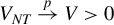 and
$T^{-1}\hat {F}^{\prime }F^{0}\overset {p}{\rightarrow } Q$
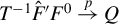 as in Bai (Reference Bai2003) and Assumption 6.
(ii) By Lemma A.6(ii) and Theorem 3.4(i),

where the third line follows from the fact that
$H\overset {p}{\rightarrow } Q^{-1}$
 as in Bai (Reference Bai2003) and Assumption 6.
(iii) By Lemma A.6(iii) and Theorem 3.4(i) and (ii),

Following the arguments as used in the proof of Theorem 3 in Bai (Reference Bai2003), we can show that
$\left (V_{1,it}+V_{2,it}\right ) ^{-1/2}(\hat {\lambda } _{i}^{\prime }\hat {f}_{t} -\lambda _{i}^{0\prime }f_{t}^{0})\overset {d}{ \rightarrow }N\left (0,1\right ) .$

A.2 Asymptotic Analysis for Section 4
To prove Theorem 4.1, we need the following two lemmas whose proofs are given in Section S.4 of the Supplementary Material.
Lemma A.7. Suppose Assumptions 1–8 hold and
$(\sqrt {N_{1}}/T+\sqrt {T}/N_{1})\log ^{2}(N_{1}T)\rightarrow 0$
 . Then
(i)
$\hat {\tau }_{it}-\tau _{it}=u_{it}-x_{it}^{\prime }(\hat {\beta }_{i\cdot }-\dot {\beta }_{i\cdot })-[x_{it}^{\prime }-{\lambda }_{i}^{0\prime }(\Lambda ^{0\prime }\Lambda ^{0} ) ^{-1}\Lambda ^{0\prime }\mathbf {x} _{\cdot t}](\hat {\beta }_{\cdot t}-\dot {\beta }_{\cdot t}) - {\lambda } _{i}^{0\prime } (N_{1}^{-1}\Lambda ^{0\prime }\Lambda ^{0} ) ^{-1} \frac {1}{N_{1}}\sum _{j=1}^{N_{1}}\lambda _{j}^{0}u_{jt} -f_{t}^{0\prime }H \mathbb {S}_{2}S_{i,T_{0,i}}^{-1}\frac {1}{T_{0,i}} \sum _{s=1}^{T_{0,i}}z_{is}u_{is} +O_{p}(\delta _{N_{1}T}^{-2}\log ^{2}(N_{1}T))\equiv \sum _{l=1}^{5}\xi _{it,l}+O_{p}(\delta _{N_{1}T}^{-2}\log ^{2}(N_{1}T))$
 uniformly in
$i\in \left [ N\right ] \backslash \left [ N_{1}\right ] $
 and
$t\in \left [ T\right ] \backslash \lbrack T_{0,i}];$

(ii)
$\frac {1}{T_{0,i}}\sum _{t=1}^{T_{0,i}}\xi _{it}x_{it}^{\prime }(\hat { \beta }_{\cdot t}-\dot {\beta }_{\cdot t})=O_{P}(\delta _{N_{1}T}^{-2}\log ^{2}\left (N_{1}T\right ) )$
 uniformly in i for
$\xi _{it}=x_{it}, f_{t}^{0}$
 and 1;
(iii)
$\frac {1}{N_{1}T_{0,i}}\sum _{j=1}^{N_{1}}\sum _{t=1}^{T_{0,i}}\lambda _{j}^{0}x_{jt}^{\prime }(\hat {\beta }_{\cdot t}-\dot {\beta }_{\cdot t})=O_{P}(\delta _{N_{1}T}^{-2}\log ^{2}\left (N_{1}T\right ) )$
 uniformly in
$i;$

(iv)
$\frac {1}{\sqrt {\left \vert \mathcal {G}_{t}\right \vert }}\sum _{i\in \mathcal {G}_{t}}x_{it}^{\prime }(\hat {\beta }_{i\cdot }-\dot {\beta }_{i\cdot })=o_{P}\left (1\right ) $
 as
$\left \vert \mathcal {G}_{t}\right \vert \rightarrow \infty ;$

(v)
$\frac {1}{\sqrt {\left \vert \mathcal {G}_{t}\right \vert }}\sum _{i\in \mathcal {G}_{t}}S_{i,T_{0,i}}^{-1}\frac {1}{T_{0,i}} \sum _{s=1}^{T_{0,i}}z_{is}u_{is}=o_{P}(1)$
 as
$\left \vert \mathcal {G} _{t}\right \vert \rightarrow \infty .$

Lemma A.8. Let
$\xi _{it,l}, l=2,\ldots ,5,$
 be as defined in Lemma A.7(i). Suppose Assumptions 1–8 hold and
$(\sqrt { N_{1}}/T+\sqrt {T}/N_{1})\log ^{2}(N_{1}T)\rightarrow 0$
 . Then
(i)
$\bar {\xi }_{2NT}\equiv \frac {1}{\sqrt {N_{2}\bar {T}_{1}}} \sum _{i=N_{1}+1}^{N}\sum _{t=T_{0,i}+1}^{T}\xi _{it,2}=-\frac {1}{\sqrt {N_{2}}} \sum _{i=N_{1}+1}^{N}\frac {T_{1,i}}{\sqrt {T_{0,i}\bar {T}_{1}}}\mu _{i\cdot ,x}^{\prime } \mathbb {S}_{1}S_{i}^{-1}\frac {1}{\sqrt {T_{0,i}}} \sum _{t=1}^{T_{0,i}}z_{it}u_{it} +o_{P}(1);$

(ii)
$\bar {\xi }_{3NT}\equiv \frac {1}{\sqrt {N_{2}\bar {T}_{1}}} \sum _{i=N_{1}+1}^{N}\sum _{t=T_{0,i}+1}^{T}\xi _{it,3}=o_{P}(1);$

(iii)
$\bar {\xi }_{4NT}\equiv \frac {1}{\sqrt {N_{2}\bar {T}_{1}}} \sum _{i=N_{1}+1}^{N}\sum _{t=T_{0,i}+1}^{T}\xi _{it,4}=o_{P}(1);$

(iv)
$\bar {\xi }_{5NT}\equiv \frac {1}{\sqrt {N_{2}\bar {T}_{1}}} \sum _{i=N_{1}+1}^{N}\sum _{t=T_{0,i}+1}^{T}\xi _{it,5}=-\frac {1}{\sqrt {N_{2}}} \sum _{i=N_{1}+1}^{N}\frac {T_{1,i}}{\sqrt {T_{0,i}\bar {T}_{1}}}\mu _{f}^{\prime }H \mathbb {S}_{2}S_{i,T_{0,i}}^{-1} \frac {1}{\sqrt {T_{0,i}}} \sum _{s=1}^{T_{0,i}}z_{is}u_{is} +o_{P}(1).$

Proof of Theorem 4.1
(i) By Lemma A.7(i), we have that uniformly in
$i\in \left [ N\right ] \backslash \left [ N_{1}\right ] $
 and
$t\in \left [ T\right ] \backslash \lbrack T_{0,i}],$


Then

It suffices to study each term in the last summation. First,
$\bar {\xi } _{i\cdot ,1T}=\frac {1}{\sqrt {T_{1,i}}}\sum _{t=T_{0,i}+1}^{T}u_{it}\overset {d} {\rightarrow }N(0,\sigma _{i\cdot ,u}^{2})$
 by Assumption 8(iv). For
$\bar {\xi }_{i\cdot ,2T}$
 and
$\bar {\xi }_{i\cdot ,5T},$
 we have, by Theorem 3.4(i),

By Lemma A.7(ii) and (iii),

In addition,
$\bar {\xi }_{i\cdot ,4T}=-{\lambda }_{i}^{0\prime }\left (N_{1}^{-1}\Lambda ^{0\prime }\Lambda ^{0}\right ) ^{-1}\frac {1}{N_{1}\sqrt { T_{1,i}}}\sum _{t=T_{0,i}+1}^{T}\sum _{j=1}^{N_{1}}\lambda _{j}^{0}u_{jt}=o_{P}(1)$
 under our assumptions. It follows that

where we recall that
$S_{i}=$
 plim
$_{T_{0,i}\rightarrow \infty }S_{i,T_{0,i}}. $
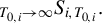
(ii) For any
$t\geq \min _{i}T_{0,i}+1,$
 we have, by Lemma A.7(i),

Note that
$\bar {\xi }_{\cdot t,1N}=\frac {1}{\sqrt {\left \vert \mathcal {G} _{t}\right \vert }}\sum _{i\in \mathcal {G}_{t}}u_{it}\overset {d}{\rightarrow } N\left (0,\sigma _{\cdot t,u}^{2}\right ) $
 by Assumption 8(v). For
$\bar {\xi }_{\cdot t,3N}$
 and
$\bar {\xi }_{\cdot t,4N},$
 we have, by Theorem 3.4(ii),

where
$r_{\cdot t}=\lim _{\left (\left \vert \mathcal {G}_{t}\right \vert ,N_{1}\right ) \rightarrow \infty }\left \vert \mathcal {G}_{t}\right \vert /N_{1}, \nu _{\cdot t,x\lambda }^{\prime }= $
 plim
$_{\vert \mathcal {G} _{t}\vert \rightarrow \infty }\frac {1}{\left \vert \mathcal {G} _{t}\right \vert }\sum _{i\in \mathcal {G}_{t}}[x_{it}^{\prime }-{\lambda } _{i}^{0\prime }(\Lambda ^{0\prime }\Lambda ^{0}) ^{-1} \Lambda ^{0\prime }\mathbf {x}_{\cdot t}],$
 and
$\mathbf {s}_{\cdot t}^{0}= $
 plim
$ _{N_{1}\rightarrow \infty }\frac {1}{N_{1}}\mathbf {x}_{\cdot t}^{\prime } \mathbb {M}_{\Lambda ^{0}}\mathbf {x}_{\cdot t}.$
 By Lemma A.7 (iv) and (v),
$\bar {\xi }_{\cdot t,2N}=-\frac {1}{\sqrt {\left \vert \mathcal {G} _{t}\right \vert }}\sum _{i\in \mathcal {G}_{t}}x_{it}^{\prime }(\hat {\beta } _{i\cdot }-\dot {\beta }_{i\cdot })=o_{P}(1),$
 and
$\bar {\xi }_{\cdot t,5N}=-f_{t}^{0\prime }H\mathbb {S}_{2}\frac {1}{\sqrt {\left \vert \mathcal {G} _{t}\right \vert }}\sum _{i\in \mathcal {G}_{t}}S_{i,T_{0,i}}^{-1}\frac {1}{ T_{0,i}} \sum _{s=1}^{T_{0,i}}z_{is}u_{is}=o_{P}(1).$
 In sum, we have

where we recall that
$\pi _{t,x\lambda }^{\prime }=$
 plim
$_{N_{1}\rightarrow \infty }\mathbf {x}_{\cdot t}^{\prime }\Lambda ^{0}(\Lambda ^{0\prime }\Lambda ^{0})^{-1}$
 and
$\Xi _{\cdot t}=\lim _{N_{1}\rightarrow \infty } \frac {1}{N_{1}}\sum _{j=1}^{N_{1}} E\{[\nu _{\cdot t,x\lambda }^{\prime }\left (\mathbf {s}_{\cdot t}^{0}\right ) ^{-1}(x_{jt}-\pi _{t,x\lambda }^{\prime }\lambda _{j}^{0}) -\mu _{\lambda }^{\prime }\Sigma _{\Lambda }^{-1}\lambda _{j}^{0}]u_{jt}\}^{2}.$

(iii)
$\bar {T}_{1}\rightarrow \infty $
 and
$N_{2}$
 is either fixed or diverge to infinity such that
$N_{2}\bar {T}_{1}=o(\delta _{N_{1}T}^{4}[\log (N_{1}T)]^{-2})$
 and
$N_{2}\log N=o\left (\underline {T}_{0}\right ) ,$


By Lemma A.8(i)–(iv),

where
$\Xi =\lim _{\left (N,T\right ) \rightarrow \infty }\frac {1}{N_{2}} \sum _{i=N_{1}+1}^{N}\alpha _{i\cdot }\frac {1}{T_{0,i}}\sum _{t,s=1}^{T_{0,i}}E \left [ z_{it}z_{is}^{\prime }u_{it}u_{is}\right ] \alpha _{i\cdot }^{\prime }, \alpha _{i\cdot }=\lim _{T\rightarrow \infty }\alpha _{i,T},$
 and
$ \alpha _{i,T}=\frac {T_{1,i}}{\sqrt {T_{0,i}\bar {T}_{1}}}(\mu _{i\cdot x,}^{\prime }\mathbb {S}_{1}+\mu _{f}^{\prime }H\mathbb {S} _{2})S_{i,T_{0,i}}^{-1}. $

SUPPLEMENTARY MATERIAL
The supplementary material for this article can be found at https://doi.org/10.1017/S0266466626100620.
FUNDING STATEMENT
X.L. acknowledges support from the Hong Kong Research Grants Council (RGC) under Grant Number 14500022 and the Chinese University of Hong Kong for the start-up fund. K.M. acknowledges the financial support from the National Natural Science Foundation of China (NSFC) under Grant Numbers 72573042 and 72121002. L.S. thanks the NSFC for financial support under Grant Number 72133002.
COMPETING INTEREST STATEMENT
The authors declare that no competing interests exist.