





1. Introduction
Given a complete manifold (M,g), one of the general themes in Riemannian geometry is to characterize the topology of M under curvature conditions on the metric g. An important theorem of Cheeger [Reference CheegerChe70] shows that there are only finitely many diffeomorphism types for non-collapsed compact manifolds with bounded curvature and diameter. There have been many efforts to generalize Cheeger’s finiteness theorem to weaker curvature assumptions. Relaxing the pointwise control
 $\|\mathrm{Rm}\|_{L^\infty}$
to an integral bound
 $\|\mathrm{Rm}\|_{L^p}$
has attracted much attention. The case
 $p=n/2,$
which we call bounded curvature concentration, is particularly interesting since the integral is scaling invariant without being weighted by the volume. The integral bound of curvature also appears naturally in many geometric problems. Perhaps more importantly, integral curvature bounds naturally arise in studying singular spaces as a weak formulation of curvature. For instance, they play an important role in the RCD theory and positive-mass theorems on asymptotically flat manifolds with singularities. One naturally asks what geometric and topological results can be extended to integral curvature bounds.
There have been many interesting generalizations of comparison geometry in this direction (see, e.g., [Reference Petersen and WeiPW97, Reference Petersen and WeiPW01, Reference CarronCar19] and the references therein). An integral curvature bound is, however, not strong enough to constrain the topology in general. Indeed, it has been shown by Yang [Reference YangYan92] that the exact analogy of Cheeger’s finiteness cannot be true in the case
 $p\lt+\infty$
, due to the failure to control the volume locally. There is a gap phenomenon, as already observed in [Reference GallotGal88, Reference YangYan92, Reference Petersen and WeiPW97, Reference Petersen and WeiPW01] (for a survey of more results in this direction, see [Reference Dai and WeiDW12, § 5]).
In this work, we are particularly interested in the gap phenomenon and compactness under the scaling-invariant curvature control
 $\|\mathrm{Rm}\|_{L^{n/2}(M)}\lt+\infty$
. In Ricci geometry, this condition has been studied extensively in the literature (for examples, see [Reference AndersonAnd89, Reference AndersonAnd90, Reference Anderson and CheegerAC91, Reference Bando, Kasue and NakajimaBKN89, Reference NakajimaNak88]). In [Reference CheegerChe03], Cheeger systemically studied the singularities of the Gromov–Hausdorff limit of non-collapsed manifolds with Ricci lower bounds and integral curvature control. Particularly when
 $p=n/2$
, Cheeger showed that the singularities must be isolated and the tangent cone at a singular point must be the cone over a quotient of the round sphere. One of the key ingredients is to prove an epsilon regularity result for a non-collapsed manifold with small curvature concentration. The method of Cheeger is elliptic, based on harmonic functions.
It is natural to ask if a metric with a sufficiently small integral curvature can be perturbed to a metric with a pointwise curvature bound in suitable topology, in order to study geometric compactness with only an integral curvature bound. To the best of our knowledge, the smoothing by Ricci flow has first been considered by Yang [Reference YangYan92]. The Ricci flow is a one-parameter family of metrics g(t) on a manifold such that
 \begin{align*}\partial_t g(t)=-2\operatorname{Ric}(g(t)).\end{align*}
Viewed as a nonlinear geometric heat equation, the flow has been proven useful to regularize metrics and obtain striking consequences in geometry and topology. When both
 $\|\mathrm{Rm}\|_{L^{n/2}}$
and
 $\|\mathrm{Ric}\|_{L^p},p\gt n/2,$
are small, Yang [Reference YangYan92] has used the Ricci flow to show that the metric can be perturbed in the
 $C^0$
topology to a metric with bounded geometry. However, the
 $C^0$
perturbation is not expected in general if one only has a scaling-invariant curvature bound, which can be seen from the point of view of tangent cones.
In [Reference Chan, Huang and LeeCHL24], the first-named author with Chan and Huang have considered a parabolic approach to Cheeger’s epsilon regularity theorem. In short, non-collapsed metrics with Ricci lower bounds and small local curvature concentration can be regularized by Ricci flow for a uniform short time with instantaneous bounded geometry. The perturbation is in the (pointed) Gromov–Hausdorff topology, in the presence of Ricci lower bounds by the distance estimate of [Reference Tian and WangTW15]. This has improved and sharpened the result of Yang [Reference YangYan92]. It is based on constructing distance-like functions with critical integral Hessian estimates, using comparison geometry, so as to construct approximating Ricci-flow solutions with suitable control. This smoothing result has later been utilized by the first-named author and Chan [Reference Chan and LeeCL24] to prove a metric gap theorem of manifolds with
 $\operatorname{Ric}\geq 0$
, Euclidean volume growth, and small curvature concentration (see also [Reference MartensMar25a]). The proof in [Reference Chan, Huang and LeeCHL24] relies on the Schoen–Yau construction of proper functions, which uses Bochner’s formula for eigenfunctions. The Ricci-curvature lower bound is crucial here in obtaining gradient estimates.
In this work, we further advance the results in [Reference Chan, Huang and LeeCHL24, Reference MartensMar25b] and show that the local smoothing holds in a greater generality. In particular, we show that the assumption of Ricci-curvature lower bounds of any kind is redundant.
Theorem 1.1.
For
 $n\geq 3$
and
 $v_0,C_s\gt0$
, there exist
 $\delta_1(n,v_0,C_s),\Lambda_1(n,v_0,C_s),L(n,v_0,C_s)$
,
 $r_1(n,v_0,C_s),$
and
 $ \hat T(n,v_0,C_s)\gt0$
, such that the following holds. Let
 $(M^n,g_0)$
be a manifold such that
 $B_{g_0}(x_0,3+\bar r)\Subset M$
for some
 $(x_0,\bar r)\in M\times [0,+\infty)$
. Suppose that for all
 $x\in B_{g_0}(x_0,2+\bar r)$
:
-
(a)
 $ \mathrm{Vol}_{g_0}(B_{g_0}(x,r))\leq v_0 r^n$
for all
$r\in (0,1]$
;
-
(b) for all
$u\in W^{1,2}_0( B_{g_0}(x,1), g_0)$
, and
\begin{align*}\bigg(\int_{ B_{g_0}(x,1)}u^{{2n}/({n-2})}\,d\mathrm{vol}_{g_0}\!\bigg)^{\!({n-2})/{n}}\leq C_s \int_{ B_{g_0}(x,1)} (|\nabla u|^2+u^2)\, d\mathrm{vol}_{g_0};\end{align*}
-
(c)
$\|\mathrm{Rm}(g_0)\|_{L^{n/2}(B_{g_0}(x,1),g_0)}\leq \varepsilon$
for some
$\varepsilon\in (0,\delta_1]$
.


Then there exists a smooth Ricci-flow solution g(t) defined on
 $B_{g_0}(x_0,1+\bar r)\times [0,\hat T]$
such that
 $g(0)=g_0$
and:
-
(1)
$ |\mathrm{Rm}(g(t))|\leq \Lambda_1 t^{-1}(\varepsilon+t^{2/n})\leq 1/({4(n-1))}t^{-1}$
; -
(2)
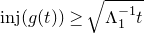
$\mathrm{inj}(g(t))\geq \sqrt{\Lambda_1^{-1} t}$
; -
(3)
$ \|\mathrm{Rm}(g(t))\|_{L^{n/2}(B_{g(t)}(x,1/2))}\leq \Lambda_1 (\varepsilon +t^{2/n}) $
; and
-
(4)
$\nu (B_{g(t)}(x,2L\sqrt{\hat T},g(t), L^2\hat T)\geq -\Lambda_1$



for all
 $(x,t)\in B_{g_0}(x_0,1+\bar r)\times (0,\hat T]$
. Moreover, for all
 $x,y\in B_{g_0}(x_0,r_1)$
and
 $ t\in [0,\hat T]$
,
 \begin{align*} \Lambda_1^{-1} [d_{g(t)}(x,y)]^{{1}/({1-2(n-1)\Lambda_1\varepsilon})}\leq d_{g_0}(x,y)\leq \Lambda_1 [d_{g(t)}(x,y)]^{{1}/({1+2(n-1)\Lambda_1\varepsilon})}.\end{align*}
Remark 1.2. The entropy lower bound measures the optimal constant of the log-Sobolev inequality. In terms of boundedness, this is equivalent to a (weighted) Sobolev constant (for an example, see [Reference Chan, Chen and LeeCCL22, Reference YeYe15]).
From the instantaneous curvature bound of g(t), Theorem 1.1 provides a local coordinate for
 $g_0$
quantitatively such that the distance is locally bi-Hölder equivalent to the Euclidean space. The smoothing is purely local in nature and does not require any local pointwise curvature bound. We use it to consider Ahlfors n-regular compact manifolds with bounded diameters, Sobolev constants, and curvature concentration. We use the local smoothing to show that the Gromov–Hausdorff limit of a sequence of manifolds in this collection must be a topological manifold away from finitely many points.
Theorem 1.3.
Let
 $n\geq 3$
and let
 $C_s,v_0,\Lambda_0,D_0\gt0$
. Suppose that
 $(M^n_i,g_i)$
is a sequence of compact manifolds such that
-
(a) for all
$u\in W^{1,2}(M_i)$
,
\begin{align*}\bigg(\int_{M_i}u^{{2n}/({n-2})}\,d\mathrm{vol}_{g_i}\!\bigg)^{\!({n-2})/{n}}\leq C_s\int_{M_i} (|\nabla u|^2+ u^2) \,d\mathrm{vol}_{g_i};\end{align*}
-
(b)
$\mathrm{Vol}_{g_i}(B_{g_i}(x,r))\leq v_0r^n$
for all
$(x,r)\in M_i\times (0,1]$
; -
(c)
$\|\mathrm{Rm}(g_i)\|_{L^{n/2}(M_i)}\leq \Lambda_0$
; -
(d)
$\mathrm{diam}(M_i)\leq D_0$
.






Then there exists a compact metric space
 $(X,d_\infty)$
and
 $\mathcal{S}=\{p_i\}_{i=1}^N$
such that
 $(M_i,g_i)$
converges subsequentially to
 $(X,d_\infty)$
in the Gromov–Hausdorff topology and
 $X\setminus \mathcal{S}$
is a topological manifold.
In the presence of Ricci lower bounds, the Sobolev constant can be ensured by volume non-collapsing. Thus, this theorem can be viewed as a generalization of results in Ricci geometry (see the compactness results in [Reference AndersonAnd89, Reference AndersonAnd90, Reference Bando, Kasue and NakajimaBKN89]). In particular, we extend the related compactness to cases without Ricci control. When
 $\Lambda_0$
is sufficiently small, the singular set
 $\mathcal{S}$
is empty and the limit X admits a smooth structure by the Ricci-flow smoothing in Theorem 1.1 (see [Reference Chan, Chen and LeeCCL22, Theorem 1.4]). It is, however, unclear to us if this is the case in general (see Remark 4.5). In the presence of Ricci-curvature lower bounds, it is also known that the tangent cone at
 $p\in \mathcal{S}$
is given by
 $C(\mathbb{S}^{n-1}/\Gamma)$
by the deep work of Cheeger [Reference CheegerChe03]. This plays an important role in the recent work of Jiang and Wei [Reference Jiang and WeiJW25] on the finiteness of diffeomorphisms. It will be interesting to know if the finite diffeomorphism theorem in [Reference Jiang and WeiJW25] can be generalized to the case without the Ricci-curvature assumption. This is related to identifying the asymptotic behavior near a singular point
 $p\in \mathcal{S}$
.
Another application of Theorem 1.1 is about complete non-compact geometry and is related to the case without singularities. We consider the topological gap phenomenon of complete non-compact manifolds with small curvature concentration. The problem has been studied by many authors (see, e.g., [Reference Cheeger and ColdingCC97, Reference LedouxLed99, Reference XiaXia99, Reference XiaXia01, Reference CheegerChe03, Reference ChenChe22, Reference Chan, Huang and LeeCHL24, Reference Chau and MartensCM26b] and the references therein). We show that a manifold with small curvature concentration is diffeomorphic to the Euclidean space provided that it supports a Euclidean-type Sobolev inequality and has Euclidean volume growth. This does not rely on the Ricci curvature and thus extends the results in [Reference Chan, Huang and LeeCHL24, Reference CheegerChe03].
Theorem 1.4.
For
 $n\geq 3$
and
 $C_s,v_0\gt0$
, there exists
 $ \delta_0(n,C_s,v_0)\gt0$
such that the following is true. Suppose that
 $(M^n,g_0)$
is a complete non-compact manifold such that:
-
(a) for all
$u\in W^{1,2}_0(M)$
,
\begin{align*}\bigg(\int_M u^{{2n}/({n-2})}\,d\mathrm{vol}_{g_0} \!\bigg)^{\!({n-2})/{n}}\leq C_s \int_M |\nabla u|^2\,d\mathrm{vol}_{g_0};\end{align*}
-
(b)
$\mathrm{Vol}_{g_0}(B_{g_0}(x,r))\leq v_0r^n$
for all
$(x,r)\in M\times \mathbb{R}_+$
; and
-
(c)
$\|\mathrm{Rm}(g_0)\|_{L^{n/2}(M)}\leq \delta_0(n,C_s,v_0)$
.




Then M is diffeomorphic to
 $\mathbb{R}^n$
.
The Sobolev condition plays a strong role in non-collapsing. It is also easily seen from the Eguchi–Hanson metric that smallness on
 $\|\mathrm{Rm}\|_{L^{n/2}}$
is necessary. It is, however, unclear if this is still necessary when n is odd.
When the negative part of Ricci curvature has a stronger decay, the volume-growth condition holds automatically by the work of Carron [Reference CarronCar19, Theorem B]. It will be interesting to know if it is necessary to assume (b) a priori in Theorem 1.4 (cf. [Reference Chau and MartensCM26a] for the case of bounded curvatures).
A natural collection to consider is the class of Euclidean submanifolds. Based on the Sobolev inequality of Michael and Simon [Reference Michael and SimonMS73], a complete Euclidean submanifold with small total curvature satisfies the Euclidean-type Sobolev inequality. Thus, Theorem 1.4 implies that such a submanifold is diffeomorphic to
 $\mathbb{R}^n$
if its volume growth is Euclidean. Moreover, when the submanifold is a convex hypersurface in
 $\mathbb{R}^{n+1},$
one can remove the volume-growth assumption and use the main theorem in [Reference Chan and LeeCL24] to show that the hypersurface is isometric to
 $\mathbb{R}^n$
when it has small total curvature. In general, in Theorem 1.4, when the scalar curvature is, furthermore, assumed to be non-negative, we expect to get a stronger rigidity result as in the Euclidian case (see Remark 5.4).
We organize the paper as follows. Section 2 provides the necessary a priori estimates that we will need in § 3, in which the main local-smoothing result (Theorem 1.1) is proven. We prove the compactness theorem (Theorem 1.3) in § 4 and the topological gap theorem (Theorem 1.4) in § 5.
2. A priori estimates of Ricci flow
In this section, we will derive some a priori estimates of the Ricci flow, this being related to the curvature concentration.
Along the Ricci flow, it is more common to consider the log-Sobolev constant, which is measured by the
 $\nu$
-entropy. Due to the celebrated work of Perelman [Reference PerelmanPer02], it is well-known that the
 $\nu$
-entropy is monotone along a complete Ricci flow with bounded curvature (see also the complete non-compact case by Chau, Tam, and Yu [Reference Chau, Tam and YuCTY11]). We need a localized version by Wang [Reference WangWan18]. Following [Reference WangWan18], for a connected domain
 $\Omega$
with possibly empty boundary in M, we define
 \begin{align*}\left\{\begin{array}{l}D_g(\Omega):=\{u\in W^{1,2}_0(\Omega): u\geq 0 \text{ and }\|u\|_{L^2(\Omega)}=1\},\\[9pt]W(\Omega, g, u, \tau):=\displaystyle\int_{\Omega}(\tau(\mathcal{R}\cdot u^2+4|\nabla u|^2)-2u^2\log u) \, d\mathrm{vol}_g -\displaystyle\frac{n}{2}\log(4\pi\tau)-n,\\[12pt]\nu(\Omega, g, \tau):= \inf\limits_{u\in D_g(\Omega), s \in (0, \tau]}W(\Omega, g, u, s),\end{array}\right.\end{align*}
where
 $\mathcal{R}$
denotes the scalar curvature.
The local entropy
 $\nu(\Omega,g,\tau)$
measures the optimal (weighed) log-Sobolev constant of
 $\Omega$
in scale of
 $\tau$
with respect to g. This also controls the Sobolev constant in some suitable scale by [Reference MartensMar25a, Lemma 3.3], which is built on [Reference YeYe15]. If g(t) is a complete Ricci flow on
 $\Omega$
with bounded curvature, it is well-known that
 $\nu(\Omega,g(t),\tau-t)$
is monotonically non-decreasing in t, again by the celebrated work of Perelman [Reference PerelmanPer02].
Although the (almost) monotonicity of the (localized)
 $\nu$
-entropy does not necessarily hold for incomplete local Ricci-flow solutions, we will construct local solutions in such a way that the entropy is still under control.
In this section, we will derive a priori estimates, assuming a bound on the localized entropy. We first need a local persistence of local curvature concentration, which is an essential key to the semi-preservation of small curvature concentration (see [Reference Chan, Chen and LeeCCL22, Reference Chan, Huang and LeeCHL24, Reference Chan and LeeCL24, Reference Chau and MartensCM26a, Reference Chau and MartensCM26b, Reference MartensMar25a, Reference MartensMar25b, Reference ChenChe22]). We need the following localized version of [Reference Chan and LeeCL24, Lemma 2.2].
Lemma 2.1 For all
 $A,{\alpha}\gt0$
, there exist
 $\delta_1(n,A)\in (0,1)$
,
 $\tilde T(n,{\alpha}),C_1(n)\gt0$
such that the following is true. Suppose that g(t) is a smooth solution to the Ricci flow on
 $M\times [0,T]$
and
 $x_0\in M$
such that for all
 $t\in [0,T]$
:
-
(a)
$B_{g(t)}(x_0,2)\Subset M$
; -
(b)
$\|\mathrm{Rm}(g(t))\|_{L^{n/2}(B_{g(t)}(x_0,2),g(t))}\lt\delta_0$
for some
$\delta_0\leq \delta_1$
; -
(c)
$\nu(B_{g(t)}(x_0,2),g(t),1)\geq -A$
; and -
(d)
$\operatorname{Ric}(g(t))\leq {\alpha} (n-1)t^{-1}$
.





Then, for all
 $t\in [0,T\wedge\tilde T]$
, we have
 \begin{align*}\int_{B_{g(t)}(x_0,1)}|\mathrm{Rm}(g(t))|^{n/2}\, d\mathrm{vol}_{g(t)} \leq \int_{B_{g_0}(x_0,2)}|\mathrm{Rm}(g_0)|^{n/2}\, d\mathrm{vol}_{g_0}+ C_1\delta_0^{n/2} t.\end{align*}
Proof. Let
 $\varphi(s)$
be a smooth non-increasing function on
 $[0,+\infty)$
such that
 $\varphi\equiv 1$
on [0, 1], vanishes outside [0, 2], and satisfies
 $|\varphi'|^2\leq 10^3\varphi$
and
 $\varphi''\geq -10^3\varphi$
. Let
 \begin{align*}\eta(x,t):=d_{g(t)}(x,x_0)+2({\alpha}+1)(n-1) \sqrt{t}\end{align*}
and define
 $\phi(x,t):=e^{-10^3t}\varphi(\eta(x,t))$
for
 $x\in B_{g(t)}(x_0,2)$
and
 $t\in [0,T]$
. It follows from [Reference PerelmanPer02, Lemma 8.3] that there exists
 $\tilde T=\tilde T(n,{\alpha})\gt0$
such that
 \begin{align*}\bigg(\frac{\partial}{\partial t}-\Delta_{g(t)}\!\bigg) \phi \leq 0\end{align*}
for
 $t\in [0,T\wedge \tilde T]$
, in the barrier sense (for a detailed discussion, see also [Reference Simon and ToppingST22, Lemma 7.1]). The inequality also holds in the distribution sense by [Reference Mantegazza, Mascellani and UraltsevMMU14, Appendix A].
Furthermore,
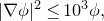 $|\nabla\phi|^2\leq 10^3 \phi,$
so that [Reference Chan, Chen and LeeCCL22, Lemma 2.1] implies
 \begin{align*}\displaystyle\frac{d}{dt} \int_M \phi^2 |\mathrm{Rm}|^{n/2}\,d\mathrm{vol}_{g(t)}&\leq -C_0^{-1} \int_M |\nabla (\phi |\mathrm{Rm}|^{n/4})|^2 d\mathrm{vol}_{g(t)}\\&\quad +C_0\int_M \phi^2 |\mathrm{Rm}|^{n/2+1} \,d\mathrm{vol}_{g(t)}\\&\quad +C_0\int_M \phi |\mathrm{Rm}|^{n/2} \,d\mathrm{vol}_{g(t)}\\&:=-\mathbf{I}+\mathbf{II}+\mathbf{III}\end{align*}
for some dimensional constant
 $C_0(n)\gt0$
. We note that the evolution equation in [Reference Chan, Chen and LeeCCL22, Lemma 2.1] is purely local, and thus the completeness of the solution there is not necessary.
Since
 $\phi(\cdot,t)$
is compactly supported on
 $B_{g(t)}(x_0,2)$
for each
 $t\in [0,T]$
,
 \begin{align*}\mathbf{III}\leq C_0\delta_0^{n/2}.\end{align*}
Similarly, together with Hölder’s inequality, we have
 \begin{align*}\mathbf{II}&\leq C_0\|\mathrm{Rm}\|_{L^{n/2}(B_{g(t)}(x_0,2))}\cdot \bigg( \int_M \phi^{{2n}/({n-2})}|\mathrm{Rm}|^{{n^2}/({2(n-2)})}\,d\mathrm{vol}_{g(t)}\!\bigg)^{\!({n-2})/{n}}\\&\leq C_0\delta_0 \cdot \bigg( \int_M \phi^{{2n}/({n-2})}|\mathrm{Rm}|^{{n^2}/({2(n-2)})}\,d\mathrm{vol}_{g(t)}\!\bigg)^{\!({n-2})/{n}}.\end{align*}
It remains to handle
 $\mathbf{I}$
. For any
 $t\in [0,T\wedge \tilde T]$
, we apply [Reference MartensMar25a, Lemma 3.3(2)] with
 $\Omega=B_{g(t)}(x_0,2)$
,
 $g=g(t)$
and
 $\tau=1$
to deduce that for some
 $\Lambda_0(n,A)\gt0$
, we have
 \begin{align}\bigg(\int_{B_{g(t)}(x_0,2)} |u|^{{2n}/({n-2})}\,d\mathrm{vol}_{g(t)} \!\bigg)^{\!({n-2})/{n}}\leq \Lambda_0 \int_{B_{g(t)}(x_0,2)} (|\nabla u|^2+ u^2) \,d\mathrm{vol}_{g(t)}\end{align}
for all
 $u\in W^{1,2}_0(B_{g(t)}(x_0,2))$
, provided that
 $\delta_0\leq \delta_1$
and that
 $\delta_1$
is small enough depending on A. Applying (2.1) to
 $u:=\phi |\mathrm{Rm}|^{n/4}$
yields
 \begin{align*}\mathbf{I}&\geq (C_0\Lambda_0)^{-1} \bigg( \int_M \phi^{{2n}/({n-2})}|\mathrm{Rm}|^{{n^2}/({2(n-2)})}\,d\mathrm{vol}_{g(t)}\!\bigg)^{\!({n-2})/{n}}-C_0^{-1}\int_M \phi^2 |\mathrm{Rm}|^{n/2}\,d\mathrm{vol}_{g(t)}.\end{align*}
Combining the above estimates, we conclude that if
 $\delta_0\leq \delta_1\leq (C_0^2 \Lambda_0)^{-1}$
, then
 \begin{align*}&\displaystyle\frac{d}{dt} \int_M \phi^2 |\mathrm{Rm}|^{n/2}\,d\mathrm{vol}_{g(t)}\\&\quad \leq (C_0+C_0^{-1}) \delta_0^{n/2}+( C_0\delta_0-(C_0\Lambda_0)^{-1} ) \cdot \bigg( \int_M \phi^{{2n}/({n-2})}|\mathrm{Rm}|^{{n^2}/({2(n-2)}})\,d\mathrm{vol}_{g(t)}\!\bigg)^{\!({n-2})/{n}}\\&\quad \leq C_1(n)\delta_0^{n/2}.\end{align*}
The assertion follows from integrating this from the initial time slice. This completes the proof.
Remark 2.2. Here, we implicitly assume that
 $\delta_1$
is small enough so that assumption in [Reference MartensMar25a, (2), Lemma 3.3] is fulfilled.
We now show that if we have a priori scaling-invariant curvature decay in time, then assumption (b) in Lemma 2.1 will be satisfied, provided that the initial metric is quantitatively Ahlfors n-regular.
Proposition 2.3.
For all
 $A,v_0\gt1$
, there exist
 $\tilde T(n)$
,
 $\delta_0(n,v_0,A)\gt0$
and
 ${\alpha}_0(n,v_0,A) \in (0,1)$
such that the following holds. Suppose that g(t) is a smooth solution to the Ricci flow on
 $M\times [0,T]$
and
 $x_0\in M$
such that for all
 $t\in [0,T]$
, we have:
-
(a)
$B_{g(t)}(x_0,2)\Subset M$
; -
(b)
$|\mathrm{Rm}(g(t))|\leq {\alpha}_0 t^{-1}$
on
$B_{g(t)}(x_0,2)$
; -
(c)
$ \nu(B_{g(t)}(x_0,2),g(t),1)\geq -A$
; -
(d)
$\mathrm{Vol}_{g_0}( B_{g_0}(x,r))\leq v_0r^n$
for
$x\in B_{g_0}(x_0,1)$
and
$r\in (0,1]$
; and -
(e)
$\|\mathrm{Rm}(g_0)\|_{L^{n/2}(B_{g_0}(x_0,2))}\lt\delta_0$
.


Then for all
 $t\in [0,T\wedge \tilde T]$
,
 \begin{align*}\bigg(\int_{B_{g(t)}(x_0,1)} |\mathrm{Rm}(g(t))|^{n/2} \,d\mathrm{vol}_{g(t)} \!\bigg)^{\!2/n}\leq \delta_1\end{align*}
where
 $\delta_1(n,A)$
is the constant from Lemma 2.1.
Proof. In the proof, we will use
 $C_i$
to denote any dimensional constant. For
 $t\in [0,T]$
and
 $x\in B_{g(t)}(x_0,1)$
, we define
 $ \rho(x,t):= \tfrac23 (\tfrac32-d_{g(t)}(x,x_0)),$
which is
 $\tfrac23$
of the g(t)-distance from x to the boundary of
 $ B_{g(t)}(x_0,\tfrac32)$
.
Let
 $\delta_0\in (0,\delta_1)$
be a constant to be specified. We claim that
 \begin{align}\bigg(\int_{B_{g(t)}(x,\rho(x,t))} |\mathrm{Rm}(g(t))|^{n/2}\,d\mathrm{vol}_{g(t)}\!\bigg)^{\!2/n}\lt\delta_1\end{align}
for all
 $ x\in B_{g(t)}(x_0,\tfrac32)$
and
 $t\in [0,T]$
if T is smaller than a dimensional constant.
By [Reference Simon and ToppingST22, Corollary 3.3], for some
 $\tilde T(n)\gt0,$
 $ B_{g(t)}(x_0,\tfrac32)\Subset B_{g_0}(x_0,2)$
for
 $t\in [0,T\wedge \tilde T]$
and
 $\rho(x,t)\to 0$
as
 $ x\to \partial B_{g(t)}(x_0,\tfrac32)$
. Therefore, if the claim in (2.2) is not true, then there exists
 $t_1\in (0,T\wedge \tilde T]$
such that:
-
(i)
$\|\mathrm{Rm}(g(t))\|_{L^{n/2}(B_{g(t)}(x,\rho(x,t)))}\lt\delta_1$
for all
$t\in [0,t_1)$
and
$ x\in B_{g(t)}(x_0,\tfrac32)$
; and -
(ii)
$\|\mathrm{Rm}(g(t_1))\|_{L^{n/2}(B_{g(t_1)}(x_1,\rho(x_1,t_1)))}=\delta_1$
for some
$ x_1\in B_{g(t_1)}(x_0,\tfrac32)$
.




We denote
 $ \rho_1:=\rho(x_1,t_1)\leq 1$
for convenience.
Claim 2.4
There exists
 $C_0(n)\gt1$
such that for any
 ${\beta}\gt1$
, if
 ${\alpha}_0\leq C_0^{-2}{\beta}^{-2}\delta_1$
, then
 $\rho_1\geq {\beta} \sqrt{t_1}$
.
Proof of Claim 2.4. Given
 ${\beta}\gt1$
, we show that
 $\rho_1\geq {\beta}\sqrt{t_1}$
if
 ${\alpha}_0$
is sufficiently small. Suppose that this is not the case, i.e.,
 $\rho_1\leq {\beta}\sqrt{t_1}$
. By (ii) and the assumption on curvature estimates,
 \begin{align*}\delta_1^{n/2}&\leq ({\alpha} t_1^{-1})^{n/2} \cdot \mathrm{Vol}_{g(t_1)}(B_{g(t_1)}(x_1,\rho_1) )\\&\leq ({\alpha} t_1^{-1})^{n/2} \cdot \mathrm{Vol}_{g(t_1)}(B_{g(t_1)}(x_1,{\beta} \sqrt{t_1}) ).\end{align*}
By the volume comparison using
 $\operatorname{Ric}(g(t))\geq -(n-1){\alpha} t^{-1}$
and a simple scaling argument, we can estimate the volume from above as long as
 ${\alpha}_0{\beta}^2\leq 1$
, so that
 \begin{align*}\delta_1^{n/2}\leq(\tfrac12C_0{\alpha}_0^{1/2}{\beta})^{n},\end{align*}
which is impossible if
 ${\alpha}_0\leq C_0^{-2}{\beta}^{-2}\delta_1$
.
On the other hand, for all
 $x\in B_{g(t_1)}(x_1,\rho_1)$
and
 $t\in [0,t_1]$
,
 \begin{align*}\tfrac32\rho(x,t)&=\tfrac32-d_{g(t)}(x_0,x)\\&\geq \tfrac32-d_{g(t)}(x_0,x_1)-d_{g(t)}(x_1,x)\\&\geq \tfrac32-d_{g(t_1)}(x_0,x_1)-d_{g(t_1)}(x_1,x) -C_1\sqrt{{\alpha}_0 t_1}\\&\ge \rho_1-C_1\sqrt{t_1}\end{align*}
for some
 $C_1\gt1$
, where we have used [Reference Simon and ToppingST22, Corollary 3.3]. Hence, by Claim 2.4, we might assume that
 $\rho(x,t)\geq \tfrac14 \rho_1$
for all
 $x\in B_{g(t_1)}(x_1,\rho_1)$
and
 $t\in [0,t_1]$
, if
 $ {\alpha}_0\leq (4C_0C_1)^{-2}\delta_1$
. Therefore, (i) implies that
 \begin{align}\int_{B_{g(t)}(x,(1/4)\rho_1)} |\mathrm{Rm}(g(t))|^{n/2}\,d\mathrm{vol}_{g(t)} \leq \delta_1^{n/2}\end{align}
for all
 $t\in [0,t_1]$
and
 $x\in B_{g(t_1)}(x_1,\rho_1)$
.
Fix
 $z\in B_{g(t_1)}(x_1,\rho_1)$
and consider the rescaled Ricci flow
 $\tilde g(t):=\lambda^2 g(\lambda^{-2}t),t\in [0,\lambda^2 t_1]$
, where
 $\lambda =8 \rho_1^{-1}$
. By (2.3) and the assumptions, for
 $t\in [0,\lambda^2 t_1],$
the rescaled flow satisfies:
-
–
$B_{\tilde g(t)}(z,2)=B_{g(\lambda^{-2}t)}(z,\tfrac14\rho_1)\Subset M$
; -
–
$\|\mathrm{Rm}(\tilde g(t))\|_{L^{n/2}(B_{\tilde g(t)}(z,2))}\lt\delta_1$
; -
–
$\nu(B_{\tilde g(t)}(z,2),\tilde g(t),1 )\geq -A;$
and -
–
$|\mathrm{Rm}(\tilde g(t))|\leq {\alpha}_0 t^{-1}$
.


Here, we have used the monotonicity on the scale
 $\tau$
in
 $\nu$
-entropy from [Reference WangWan18, Proposition 3.2] and
 $\lambda^{-2}=8^{-2}\rho_1^2\leq 1$
.
We apply Lemma 2.1 to
 $\tilde g(t)$
to conclude that
 \begin{align*}\int_{B_{\tilde g(t)}(z,1)}|\mathrm{Rm}(\tilde g(t))|^{n/2}\, d\mathrm{vol}_{\tilde g(t)}&\leq \int_{B_{\tilde g_0}(z,2)}|\mathrm{Rm}(\tilde g_0)|^{n/2}\, d\mathrm{vol}_{\tilde g_0}+ C_2\delta_1^{n/2} t\\&\leq \delta_0^{n/2}+ C_2\delta_1^{n/2} t\end{align*}
for all
 $t\in [0,\lambda^2t_1 \wedge \tilde T(n)]$
. Rescaling it back, we conclude that
 \begin{align}\int_{B_{g(s)}(z,(1/8)\rho_1)}|\mathrm{Rm}(g(s))|^{n/2}\,d\mathrm{vol}_{g(s)} &\leq \delta_0^{n/2}+64C_2\delta_1^{n/2} \rho_1^{-2} s\nonumber\\&=: \delta_0^{n/2}+ C_3\delta_1^{n/2} \rho_1^{-2} s\end{align}
for all
 $s\in [0,t_1\wedge 8^{-2}\tilde T \rho_1^2]$
and
 $z\in B_{g(t_1)}(x_1,\rho_1)$
. By Claim 2.4, if
 \begin{align*} {\alpha}_0\leq \min\{(8C_0)^{-2}\tilde T\delta_1, (4C_1C_0)^{-2}\delta_1\},\end{align*}
then (2.4) holds at
 $s=t_1$
.
We now use (2.4) to contradict (ii), the equality at
 $(x_1,t_1)$
. By choosing a maximal collection of
 $\{z_i\}_{i=1}^N$
in
 $B_{g(t_1)}(x_1,\tfrac{39}{40}\rho_1)$
such that
 $B_{g(t_1)}(z_i,\tfrac{1}{40}\rho_1)$
are pair-wise disjoint, we have a collection of points
 $\{z_i\}_{i=1}^N$
such that
 \begin{align}\coprod_{i=1}^N B_{g(t_1)}\bigg(z_i,\frac1{40}\rho_1\!\bigg)\subseteq B_{g(t_1)}(x_1,\rho_1) \subseteq \bigcup_{i=1}^NB_{g(t_1)}\bigg(z_i,\frac18\rho_1\!\bigg).\end{align}
Then (ii) and (2.4) imply that
 \begin{align}\delta_1^{n/2}&\leq N ( \delta_0^{n/2}+ C_3\delta_1^{n/2} \rho_1^{-2}t_1 ).\end{align}
Claim 2.5.
There exist
 $\gamma_1(n,A),N_0(n,A,v_0)\gt0$
such that if
 ${\alpha}_0\leq \gamma_1\delta_1$
, then
 $N\leq N_0$
.
Proof of Claim 2.5. This follows from [Reference MartensMar25b, Lemma 2.1] (see also the proof of [Reference Chan, Chen and LeeCCL22, Theorem 1.2]). For readers’ convenience, we include its proof.
By [Reference Simon and ToppingST22, Corollary 3.3] and Claim 2.4, we might assume that
 $B_{g(t_1)}(x_1,\rho_1)\subseteq B_{g_0}(x_1,2\rho_1)$
and
 $B_{g(t_1)}(z_i,\tfrac{1}{40}\rho_1)\subseteq B_{g(s)}(z_i, \rho_1/4)$
for
 $s\in[0,t_1]$
. From (2.5) and the assumption of Ahlfors n-regularity, we have
 \begin{align}\sum_{i=1}^N\mathrm{Vol}_{g_0}\bigg(\!B_{g(t_1)}\bigg(\!z_i,\frac1{40}\rho_1\!\bigg)\! \bigg)&\leq \mathrm{Vol}_{g_0}(B_{g(t_1)}(x_1,\rho_1) )\nonumber\\&\leq \mathrm{Vol}_{g_0}(B_{g_0}(x_1,2\rho_1) )\leq v_0(2\rho_1)^n.\end{align}
It remains to control each
 $\mathrm{Vol}_{g_0}(B_{g(t_1)}(z_i,\tfrac{1}{40}\rho_1) )$
from below. We compare it with volume at
 $t=t_1$
as follows. For
 $s\in [0,t_1]$
and any i,
 \begin{align*}&\displaystyle\frac{d}{ds}\mathrm{Vol}_{g(s)}\bigg(\!B_{g(t_1)}\bigg(\!z_i,\frac1{40}\rho_1\!\bigg)\!\bigg)\\[10pt] &\quad=-\int_{B_{g(t_1)}(z_i,(1/{40})\rho_1)}\mathcal{R}(g(s))\,d\mathrm{vol}_{g(s)}\\[10pt]&\quad\leq\bigg(\int_{B_{g(t_1)}(z_i,(1/{40})\rho_1)}|\mathrm{Rm}(g(s))|^{{n}/{2}}\,d\mathrm{vol}_{g(s)}\!\bigg)^{\!2/n}\bigg[\mathrm{Vol}_{g(s)}\bigg(\!B_{g(t_1)}\bigg(\!z_i,\frac1{40}\rho_1\!\bigg)\!\bigg) \bigg]^{1-(2/n)}\\[10pt]&\quad\leq \delta_1\bigg[\mathrm{Vol}_{g(s)}\bigg(\!B_{g(t_1)}\bigg(\!z_i,\frac1{40}\rho_1\!\bigg)\!\bigg) \bigg]^{1-(2/n)} ,\end{align*}
where we have used (2.3) and
 $z_i\in B_{g(t_1)}(x_1,\rho_1)$
.
By integrating it from
 $s=0$
to
 $s=t_1$
, we conclude that
 \begin{align}\bigg[\mathrm{Vol}_{g(t_1)}\bigg(\!B_{g(t_1)}\bigg(\!z_i,\frac1{40}\rho_1\!\bigg)\! \bigg)\bigg]^{2/n}&\leq\bigg[\mathrm{Vol}_{g_0}\bigg(\!B_{g(t_1)}\bigg(\!z_i,\frac1{40}\rho_1\!\bigg)\! \bigg)\bigg]^{2/n} +\frac{2\delta_1}n t_1.\end{align}
On the other hand, by assumption (c) and the monotonicity of the
 $\nu$
-entropy (in terms of domains) [Reference WangWan18, Proposition 2.1],
 $\nu(B_{g(t_1)}(z_i,\tfrac{1}{40} \rho_1, g(t_1),1)\geq -A.$
Thus, (2.3), [Reference MartensMar25a, Lemmas 3.1 and 3.3], and Remark 2.2 imply that
 \begin{align}\mathrm{Vol}_{g(t_1)}(B_{g(t_1)}(z_i,\tfrac1{40}\rho_1))\geq \gamma_0\cdot \rho_1^n\end{align}
for some
 $\gamma_0(n,A)\gt0$
.
By Claim 2.4 with
 ${\beta}=2\gamma_0^{-1/n}$
, we then have
 \begin{align*}\gamma_0^{2/n} \rho_1^2\geq 4 t_1\gt \frac{4}{n} \delta_1 t_1\end{align*}
provided that
 ${\alpha}_0\leq C_0^{-2}\delta_1\cdot \min\{2\gamma_0^{-1/n}, 8^{-2}\tilde T\}^{ -2}=:\gamma_1(n,A) \cdot \delta_1$
. Using this with (2.9) and (2.8), we estimate the left-hand side of (2.7) by
 \begin{align*}\sum_{i=1}^N\mathrm{Vol}_{g_0}\bigg(\!B_{g(t_1)}\bigg(\!z_i,\frac1{40}\rho_1\!\bigg)\! \bigg)&\geq \sum_{i=1}^N\bigg(\gamma_0^{2/n} \rho_1^2 -\frac{2\delta_1}{n}t_1\!\bigg)^{\!n/2}\\&\geq N2^{-n/2} \gamma_0 \rho_1^n ,\end{align*}
so that
 $N\leq 4^n\gamma_0^{-1} v_0=: N_0(n,A,v_0)$
from (2.7).
We can finish the proof of Proposition 2.3. We now choose
 $\delta_0(n,v_0,A):= (4N_0)^{-2/n}\delta_1$
so that from Claim 2.5, we can deduce from (2.6) that
 \begin{align*}\rho_1^2\lt 2C_3N_0 t_1.\end{align*}
By Claim 2.4, this is impossible if we choose
 \begin{align*}{\alpha}_0:=\delta_1\cdot\min\{(8C_0)^{-2}\tilde T, \gamma_1,(4C_0C_1)^{-2}, {C_0^{-2}} (2C_3N_0)^{-1}\}.\end{align*}
This proves the claim (2.2). The proposition follows by the claim using
 $\rho(x_1,t)=1$
.
The upshot of Proposition 2.3 is that it allows us to re-apply Lemma 2.1 to obtain an improved estimate of curvature.
Proposition 2.6.
For
 $n,A\gt0$
, there exists
 $\Lambda_0(n,A)\gt0$
such that the following holds. Under the assumptions in Proposition 2.3, if, in addition, we have
 $\|\mathrm{Rm}(g_0)\|_{L^{n/2}(B_{g_0}(x_0,1))}\leq \varepsilon$
, then we have
 \begin{align*}|\mathrm{Rm}(x_0,t)|\leq \Lambda_0 t^{-1}(\varepsilon +t^{2/n})\end{align*}
for
 $t\in (0,T\wedge \tilde T]$
.
Proof. By Proposition 2.3, we have
 $\|\mathrm{Rm}(g(t))\|_{L^{n/2}(B_{g(t)}(x_0,1))}\leq \delta_1$
for
 $t\in [0,T\wedge \tilde T]$
, where
 $\delta_1(n,A)$
is the constant from Lemma 2.1. Applying Lemma 2.1 to the rescaled Ricci flow
 $\tilde g(t):= 4g(4^{-1}t),t\in [0,4(T\wedge \tilde T)]$
and then rescaling it back to g(t), we see that
 \begin{align*}\int_{B_{g(t)}(x_0,1/2 )}|\mathrm{Rm}(g(t))|^{n/2}\, d\mathrm{vol}_{g(t)}& \le \int_{B_{g_0}(x_0, 1)}|\mathrm{Rm}(g_0)|^{n/2}\, d\mathrm{vol}_{g(0)} + 4C_1\delta_1^{n/2} t\\& \leq \varepsilon^{n/2}+ 4C_1\delta_1^{n/2} t\end{align*}
for all
 $t\in [0,T\wedge\tilde T]$
. Due to the curvature assumption and the volume non-collapsing from [Reference WangWan18, Theorem 5.4], standard Moser iteration (see, e.g., [Reference LiLi12, Chapter 19]) yields
 \begin{align*}t|\mathrm{Rm}(x_0,t)|\leq \Lambda_0 (\varepsilon +t^{2/n})\end{align*}
for some
 $\Lambda_0(n,A)\gt0$
. This completes the proof.
In particular, Proposition 2.6 asserts that the Ricci flow has an improved estimate from the smallness of the initial local curvature concentration.
The next lemma states that for a complete bounded-curvature Ricci flow, the local
 $\nu$
-functional is (almost) preserved. This has first been considered by Wang [Reference WangWan18], localizing the work of Perelman [Reference PerelmanPer02]. The following refined version is by Cheng [Reference ChengChe25].
Lemma 2.7 (Lemma 2.5 in [Reference ChengChe25]). Fix
 $0\leq s_1\leq s_2\leq 1$
. Suppose that g(t) is a smooth solution to the Ricci flow on
 $M\times [s_1,s_2]$
with bounded curvature such that for all
 $t\in [s_1,s_2]$
and
 $x\in B_{g(t)}(x_0,\sqrt{t}),$
 \begin{align*}\operatorname{Ric}(g(t))\leq (n-1)\hat {\alpha} t^{-1}.\end{align*}
Then, for any
 $\tau\gt0$
,
 ${\beta}\in (0,\tfrac{1}{10}),$
and
 $\gamma\in [0,8-20{\beta})$
, we have
 \begin{align*}&\nu(\Omega_2,g(s_2),\tau+1-s_2)-\nu(\Omega_1,g(s_1),\tau+1-s_1)\\&\quad \geq -\bigg[ \frac{1+\tau}{10 \hat {\alpha}^2{\beta}^2}+\frac1e\bigg]\cdot \bigg[ \exp\bigg(\frac{s_2-s_1}{10\hat {\alpha} ^2{\beta}^2}\!\bigg)-1\bigg] ,\end{align*}
where
 \begin{align*}\left\{\begin{array}{l}\Omega_1:=B_{g(s_1)}(x_0,10\hat {\alpha} -2\hat {\alpha}\sqrt{s_1}-\hat {\alpha} \gamma );\\[3pt]\Omega_2:=B_{g(s_2)}(x_0,10\hat {\alpha} (1-2{\beta})-2\hat {\alpha} \sqrt{s_2}-\hat {\alpha} \gamma).\end{array}\right.\end{align*}
3. Local smoothing using Ricci flow
In this section, we will construct local solutions to the Ricci flow that locally regularize metrics with small local curvature concentration, i.e., Theorem 1.1. We adapt the idea of Cheng [Reference ChengChe25] with the estimates in § 2 to construct local Ricci flow, building on the idea of Hochard [Reference HochardHoc19]. To prove Theorem 1.1, we need to specify some constants precisely. We need two more ingredients. The first is a result of Hochard that allows us to construct a local Ricci flow on regions with bounded curvature.
Proposition 3.1 (Proposition 4.2 in [Reference Lee and ToppingLT25], based on [Reference HochardHoc19]). For
 $n\geq 2$
, there exist constants
 $\gamma(n)\in (0,1]$
and
 $\Lambda(n)\gt1$
so that the following is true. Suppose that
 $(N^n,h_0)$
is a smooth manifold (not necessarily complete) that satisfies
 $|\mathrm{Rm}(h_0)|\leq \rho^{-2}$
throughout, for some
 $\rho\gt0$
. Then there exists a smooth complete Ricci flow h(t) on N for
 $t\in [0,\gamma \rho^2]$
, with the properties that
-
(i)
$h(0)=h_0$
on
$N_\rho=\{x\in N: B_{h_0}(x,\rho)\Subset N\}$
; -
(ii)
$|\mathrm{Rm}(h(t))|\leq \Lambda \rho^{-2}$
throughout
$N\times [0,\gamma \rho^2]$
.


The Ricci flow obtained in [Reference Lee and ToppingLT25, Proposition 4.2] is constructed by modifying the incomplete metric at its extremities in order to make it complete, and followed by running Shi’s classical solution. Thus, the solution h(t) is by construction a complete solution on the whole N.
We also recall the shrinking-balls lemma, which is one of the local ball inclusion results based on the distance-distortion estimates of Hamilton and Perelman from [Reference PerelmanPer02, Lemma 8.3].
Lemma 3.2 [Reference Simon and ToppingST22, Corollary 3.3]. For
 $n\geq 2$
, there exists a constant
 $\beta(n)\geq 1$
such that the following is true. Suppose that
 $(N^n,g(t))$
is a Ricci flow for
 $t\in [0,S]$
and
 $x_0\in N$
with
 $B_{g(0)}(x_0,r)\Subset N$
for some
 $r\gt0$
, and
 $\operatorname{Ric}_{g(t)}\leq a(n-1)/t$
on
 $B_{g_0}(x_0,r)$
for each
 $t\in (0,S]$
. Then, for each
 $t\in (0,S],$
 \begin{align*}B_{g(t)}(x_0,r-\beta\sqrt{a t})\subseteq B_{g_0}(x_0,r).\end{align*}
We are now ready to prove Theorem 1.1.
Proof of Theorem 1.1. We first prove the existence when
 $\|\mathrm{Rm}(g_0)\|_{L^{n/2}(B_{g_0}(x_0,1),g_0)}\leq \varepsilon_1$
for
 $\varepsilon_1\gt0$
, which is fixed below. By [Reference MartensMar25a, Lemma 3.2], we might assume that
 $\nu(B_{g_0}(x,1),g_0,2 )\geq -A_0$
for some
 $A_0(n,C_s)$
, by working on a slightly smaller ball if necessary. We need to specify how the positive constants are chosen, since the precise forms of the constants will play a crucial role in the construction:
-
–
$\gamma(n)$
and
$\Lambda(n)$
from Proposition 3.1; -
–
${\beta}(n)$
from Lemma 3.2; -
–
$A:=A_0+1$
; -
–
$\tilde T(n),\delta_0(n,v_0,A)$
and
${\alpha}_0(n,v_0,A)$
from Proposition 2.3; -
–
$\Lambda_0(n,A)$
from Proposition 2.6; -
–
$\varepsilon_1(n,v_0,A):=\min\{ \delta_0, {\alpha}_0 (2\Lambda_0)^{-1}, {\alpha}_0 (4\Lambda\Lambda_0)^{-1}\}$
; -
–
$\mu(n,v_0,A):=\min\{ 10^{-2},\gamma (2\varepsilon_1 \Lambda_0)^{-1}\}$
; -
–
$\sigma(n,v_0,A):=10^{-3} (1-(1+\mu)^{-1/5} )$
; -
–
$L(n,v_0,A):=10^4{\alpha}_0^{-1/2}\cdot \max\{ {\beta},\tilde T ^{-1/2},\varepsilon_1^{-n} ,n, \mu\sigma^{-2} , \sigma^{-2}[1-(1+\mu)^{-1/5} ]^{-1}\}$
; and -
–
$\hat T(n,v_0,A):=\min\{ 10^{-1}{\alpha}_0^{-1}L^{-2},(\tfrac14 L^2{\alpha}_0+\mu+1)^{-1}\}.$





Let
 $\rho_0\in (0,\tfrac12)$
be small such that
 $|\mathrm{Rm}(g_0)|\leq \rho_0^{-2}$
on
 $N_0:=B_{g_0}(x_0,2+\bar r)$
. Then, from Proposition 3.1, there exists a smooth complete Ricci flow h(t) on
 $N_0\times [0,\gamma\rho_0^2]$
such that:
-
–
$h(0)=g_0$
on
$(N_0)_{\rho_0} := B_{g_0}(x_0,2+\bar r-\rho_0)$
; and -
–
$|\mathrm{Rm}(h(t))|\leq \Lambda \rho_0^{-2}$
on
$N_0\times [0,\gamma \rho_0^2]$
.


We choose
 $t_0:= \rho_0^2\cdot \min\{\gamma, \Lambda^{-1}{\alpha}_0\}$
so that
 \begin{align*}|\mathrm{Rm}(h(t))|\leq \Lambda \rho_0^{-2}\leq {\alpha}_0 t_0^{-1} \leq {\alpha}_0t^{-1}\end{align*}
on
 $N_0\times (0,t_0]$
. We also denote
 $t_{-1}=0$
for notional consistency. We define a sequence of times
 $t_k$
and radii
 $r_k$
inductively as follows:
-
(i)
$r_0:=2+\bar r-\rho_0$
; -
(ii)
$t_{k+1}:=(1+\mu) t_k$
for
$k\geq 0$
; and -
(iii)
$r_{k+1}=r_k-8L\sqrt{{\alpha}_0 t_k}$
for
$k\geq 0$
.


We consider the statement
 $\mathcal{P}(k)$
:
There exists a smooth Ricci flow g(t) defined on
 $B_{g_0}(x_0,r_k)\times [0,t_k]$
such that
(I)
 $g(0)=g_0$
,
(II)
 $|\mathrm{Rm}(g(t))|\leq {\alpha}_0 t^{-1}$
for
 $t\in (0,t_k]$
, and
(III)
 $ \nu(B_{ g(t)}(x,L\sqrt{{\alpha}_0 t_k}), g(t),\tfrac14 L^2 {\alpha}_0 t_k)\geq -A$
for all
 $(x,t)\in B_{g_0}(x_0,r_k)\times (0,t_k]$
.
From the above discussion, since h(t) is smooth and
 $A\gt A_0$
, we might assume that
 $\mathcal{P}(0)$
is true by shrinking
 $\rho_0$
if necessary, for instances using the continuity of entropy [Reference WangWan18, Corollary 2.5]. We want to show that
 $\mathcal{P}(k)$
is true if
 $r_k\gt0$
and
 $t_k\lt\hat T$
, both of which hold when
 $k=0$
.
We prove this by induction on k.
 $\mathcal{P}(0)$
is true by the above construction. Suppose that for some
 $k\ge 0$
with
 $r_{k+1}\gt0$
and
 $t_{k+1}\lt \hat T,$
 $\mathcal{P}(i)$
is true for
 $0\le i\le k.$
We let g(t) be the Ricci flow on
 $B_{g_0}(x_0,r_k)\times [0,t_k]$
from
 $\mathcal{P}(k)$
. We first improve the curvature estimate on a smaller domain.
Claim 3.3. We have
 \begin{align*}|\mathrm{Rm}(g(t))|\leq 2\varepsilon_1\Lambda_0t^{-1}\end{align*}
on
 $B_{g_0}(x_0,r_k-2L\sqrt{{\alpha}_0 t_k})\times [0,t_k]$
.
Proof of Claim 3.3. Let
 $z\in B_{g_0}(x_0,r_k-2L\sqrt{{\alpha}_0 t_k})$
so that Lemma 3.2 implies
 \begin{align*}B_{g(t)}(z,L\sqrt{{\alpha}_0 t_k})&\subseteq B_{g_0}(z,2L\sqrt{{\alpha}_0 t_k})\subseteq B_{g_0}(x_0,r_k)\end{align*}
for all
 $t\in [0,t_k]$
. We consider the rescaled Ricci flow
 $\tilde g(t):=\lambda^{-2}g(\lambda^2 t)$
for
 $t\in [0,\lambda^{-2}t_k]$
, where
 $\lambda=\tfrac12 L\sqrt{{\alpha}_0 t_k}$
, and denote
 $\tilde g_0:=\tilde g(0)$
. Then, for all
 $t\in [0,4L^{-2}{\alpha}_0^{-1}]$
, we have:
-
(A)
$B_{\tilde g(t)}(z,2)=B_{g(\lambda^2 t)}(z,2\lambda)\Subset M$
; -
(B)
$|\mathrm{Rm}(\tilde g(t))|\leq {\alpha}_0 t^{-1}$
on
$B_{\tilde g(t)}(z,2)$
; -
(C)
$ \nu(B_{\tilde g(t)}(z,2),\tilde g(t),1)\geq -A$
; -
(D)
$\mathrm{Vol}_{\tilde g_0}( B_{\tilde g_0}(x,r))\leq v_0r^n$
for
$x\in B_{\tilde g_0}(z,1)$
and
$r\in (0,1]$
; and -
(E)
$\|\mathrm{Rm}(\tilde g_0)\|_{L^{n/2}(B_{\tilde g_0}(z,2) , \tilde g_0)}\lt\varepsilon_1$
.




Here, we have used
 $2\lambda=L\sqrt{{\alpha}_0 t_k}\lt1$
so that
 $B_{\tilde g_0}(x,2)\subseteq B_{g_0}(x,1)$
where the initial estimates hold. The entropy lower bound (C) follows from (III):
 \begin{align*}\nu(B_{\tilde g(t)}(z,2),\tilde g(t),1)&= \nu(B_{ g(s)}(z,L\sqrt{{\alpha}_0 t_k}), g(s),\tfrac14 L^2{\alpha}_0 t_k)\geq -A\end{align*}
for
 $s=\lambda^2t\in [0,t_k]$
. Thus, the rescaled flow
 $\tilde g(t)$
satisfies all the conditions of Proposition 2.3. It follows from Proposition 2.6 and our choice of L and
 $\varepsilon_1$
that for
 $t\in (0,t_k]$
,
 \begin{align*}|\mathrm{Rm}(z,t)|\leq 2\varepsilon_1\Lambda_0 t^{-1}.\end{align*}
This proves the claim.
We now use the improved estimate from Claim 3.3 to extend the solution.
Claim 3.4.
The Ricci flow g(t) can be extended to
 $[0,t_{k+1}]$
on
 $B_{g_0}(x_0,r_k-4L\sqrt{{\alpha}_0 t_k})$
such that (I)–(II) in
 $\mathcal{P}(k+1)$
hold. Moreover, there is a complete bounded-curvature Ricci flow
 $h_k(t)$
on
 $B_{g_0}(x_0,r_k-2L\sqrt{{\alpha}_0t_k})\times [t_k,t_{k+1}]$
such that
 $|\mathrm{Rm}(h_k(t))|\leq {\alpha}_0 t^{-1}$
and
 $h_k(t)|_{B_{g_0}(x_0,r_k-4L\sqrt{{\alpha}_0 t_k})}=g(t)$
.
Proof of Claim 3.4. Denote
 ${\alpha}_1:= 2\varepsilon_1\Lambda_0\le \alpha_0$
for convenience. We apply Proposition 3.1 with a translation in time, on
 $N=N_k:=B_{g_0}(x_0,r_k-2L\sqrt{{\alpha}_0t_k})$
and
 $h_{0,k}=g(t_k)$
with
 $\rho=\rho_k:=\sqrt{{\alpha}_1^{-1}t_k}$
to obtain a complete Ricci flow
 $h_k(t)$
on
 $N_k\times [t_k,t_k+\gamma {\alpha}_1^{-1} t_k]$
such that:
-
–
$h_k(t_k)=h_{0,k}$
on
$(N_k)_{\rho_k}=\{ x \in N_k : B_{g(t_k)}(x,\rho_k)\Subset N_k \}$
; and -
–
$|\mathrm{Rm}(h_k(t))|\leq \Lambda \rho_k^{-2}= \Lambda {\alpha}_1 t_k^{-1}$
on
$N_k\times [t_k,(1+\gamma {\alpha}_1^{-1} )t_k]$
.


It remains to show that
 $(N_k)_{\rho_k}\supseteq B_{g_0}(x_0,r_{k}-4L\sqrt{{\alpha}_0 t_k})$
. Let
 $x\in B_{g_0}(x_0,r_{k}-4L\sqrt{{\alpha}_0 t_k})$
; hence we have
 $B_{g_0}(x,2L\sqrt{{\alpha}_1 t_k})\subseteq N_k$
. Due to (II) in the induction hypothesis
 $\mathcal{P}(k)$
, Lemma 3.2 implies that
 \begin{align*}B_{g(t_k)}(x,L\sqrt{{\alpha}_0 t_k})\Subset B_{g_0}(x,2L\sqrt{{\alpha}_0 t_k})\subseteq N_k ,\end{align*}
so that
 $x\in (N_k)_{\rho_k}$
. Thus,
 $h_k({ t_k})=h_{0,k}=g(t_k)$
on
 $B_{g_0}(x_0,r_{k}-4L\sqrt{{\alpha}_0 t_k})$
.
By our choice of
 $\mu$
, we know that
 $t_{k+1}-t_k=\mu t_k\leq \gamma {\alpha}_1^{-1} t_k$
. Therefore, we might patch the Ricci flow together on
 $B_{g_0}(x_0,r_k-4L\sqrt{{\alpha}_0t_k})\times [0,t_{k+1}]$
by taking
 \begin{align*}g(t):=\begin{cases} g(t)&\text{if } t\in[0, t_k], \\ h_k(t)&\text{if } t\in [t_k,t_{k+1}] .\end{cases}\end{align*}
By our choice of
 $\varepsilon_1$
, we see that for
 $t\in [t_k,t_{k+1}]$
,
 \begin{align*}|\mathrm{Rm}(g_k(t))|\leq \Lambda {\alpha}_1 t^{-1}_k& = 2\varepsilon_1 \Lambda_0\Lambda(1+\mu) t^{-1}_{k+1}\\&\leq 4\varepsilon_1 \Lambda_0\Lambda t^{-1}\leq {\alpha}_0 t^{-1}.\end{align*}
This finishes the proof of the claim.
We will assume that g(t) for
 $t\leq t_k$
, is constructed by inductively using Claim 3.4, so that on each sub-interval
 $[t_i,t_{i+1}]$
, the Ricci flow g(t) is restriction of some complete bounded-curvature Ricci flow.
It remains to show that (III) in
 $\mathcal{P}(k+1)$
holds. For each i, from Claim 3.4 and the induction hypothesis, there is a complete bounded-curvature Ricci flow
 $h_i(t)$
on
 $B_{g_0}(x_0,r_i-2L\sqrt{{\alpha}_0 t_i})\times [t_i,t_{i+1}]$
such that:
-
–
$h_i(t)|_{B_{g_0}(x_0,r_i-4L\sqrt{{\alpha}_0 t_i})}=g(t)$
; and -
–
$|\mathrm{Rm}(h_i(t))|\leq {\alpha}_0 t^{-1}$
, where
${\alpha}_0\lt 1\lt10^3n$
.



We now consider the rescaled Ricci flow
 $\tilde g(t):=t_k^{-1}g(t_k t)$
for
 $t\in [0,1+\mu]$
. For each i, we also define the rescaled Ricci flow
 $\tilde h_i(t):=t_k^{-1}h_i(t_k t)$
for
 $t\in [\tilde t_i,\tilde t_{i+1}]$
, where
 $\tilde t_i:=t_k^{-1}t_i$
. For
 $z\in B_{g_0}(x_0,r_{k+1})$
, we apply Lemma 2.7 to deduce that
 \begin{align}& \nu(B_{\tilde h_i(\tilde t_{i+1})}(z, (10(1-2\hat{\beta})- \gamma-2\sqrt{\tilde t_{i+1}}) \hat{\alpha}),\tilde h_i(\tilde t_{i+1}),\tau+1-\tilde t_{i+1} )\nonumber\\&\quad \geq \nu(B_{\tilde h_i(\tilde t_{i})}(z, (10- \gamma-2\sqrt{\tilde t_{i}}) \hat{\alpha}),\tilde h_i(\tilde t_{i}),\tau+1-\tilde t_{i})\nonumber\\&\qquad -\bigg( \frac{1+\tau}{10 \hat {\alpha} ^2\hat{\beta}^2}+\frac1e\bigg)\cdot \bigg[ \exp\bigg(\frac{\mu \tilde t_i}{10 \hat {\alpha} ^2\hat{\beta}^2}\bigg)-1\bigg]\end{align}
for any
 $\hat{\alpha}\geq 10^3n$
,
 $\tau\gt0$
,
 $\hat{\beta}\in(0,\tfrac{1}{10})$
, and
 $\gamma\in [0,8-20\hat{\beta})$
. The analogous estimate also holds if
 $\tilde t_{i+1}$
is replaced by any
 $t\in [\tilde t_i,\tilde t_{i+1}]$
.
We start to prove (III) in
 $\mathcal{P}(k+1).$
Suppose that
 $\tilde t\in [\tilde t_\ell,\tilde t_{\ell+1}]$
for some
 $-1\le \ell\le k.$
We fix
 \begin{align*}\hat{\alpha}:=5^{-1}L\sqrt{{\alpha}_0}\geq10^3n\quad\mathrm{and}\quad \tau:=\mu+\tfrac14 L^2{\alpha}_0.\end{align*}
For
 $-1\le i\le \ell,$
we define
 \begin{align*}\hat{\beta}_i&:= \sigma\cdot \tilde t_i^{1/5},\\\gamma_{i}&:=\gamma_{i-1}+20\hat{\beta}_{i-1},\end{align*}
and
 \begin{align*} \nu_i&:=\nu(B_{\tilde h_i(\tilde t_{i})}(z, (10- \gamma_i-2\sqrt{\tilde t_{i}})\hat{\alpha}),\tilde h_i(\tilde t_{i}),\tau+1-\tilde t_{i}),\end{align*}
where
 $\gamma_i$
is defined inductively starting from the final data below. Here,
 $\sigma$
is the constant defined at the beginning of the proof. Recall that we also set
 $t_{-1}:=0.$
We also define the ‘initial data’:
 \begin{align*}\hat {\beta}_{\tilde t}&:= \sigma\, \tilde t^{1/5},\\\gamma_{\tilde t}&:= 10(1-2\hat {\beta}_{\tilde t})-2\sqrt{\tilde t}-L\hat {\alpha}^{-1}\sqrt{{\alpha}_0},\,\\ \gamma_{\ell}&:= \gamma_{\tilde t}+20\hat{\beta}_{\tilde t},\end{align*}
and
 \begin{align*} \nu_{\tilde t}&:= { \nu(B_{\tilde h_{\ell}(\tilde t)}(z, (10- \gamma_{\tilde t}-2\sqrt{\tilde t})\hat{\alpha}),\tilde h_{\ell}(\tilde t),\tau+1-\tilde t).}\end{align*}
The definition of
 $\gamma_{\tilde t}$
implies that
 \begin{align}10(1-2\hat {\beta}_{\tilde t})-\gamma_{\tilde t}-2\sqrt{\tilde t}= L\hat {\alpha}^{-1}\sqrt{{\alpha}_0}=5.\end{align}
Since
 $B_{g_0}(z,4L\sqrt{{\alpha}_0t_k})\Subset B_{g_0}(x_0,r_k-4L\sqrt{{\alpha}_0t_k})$
, where
 ${ g(t)= h_i(t)}$
for
 $t\in [t_i,t_{i+1}]$
from Claim 3.4 and the remark after it, Lemma 3.2 implies that for
 $t\in [t_i,t_{i+1}]$
,
 \begin{align*}B_{ g(t)}( z,3L\sqrt{{\alpha}_0t_k} )\Subset B_{g_0}(x_0,r_i-4L\sqrt{{\alpha}_0t_i})\end{align*}
and thus,
 \begin{align*}\nu_i=\nu(B_{\tilde g(\tilde t_{i})}(z, (10- \gamma_i-2\sqrt{\tilde t_{i}})\hat{\alpha}),\tilde g(\tilde t_{i}),\tau+1-\tilde t_{i}).\end{align*}
By the monotonicity of the
 $\nu$
-entropy [Reference WangWan18, Propositions 2.1], due to
 $t_k\leq \hat T$
and our choice of
 $\hat T$
, we have
 \begin{align}\nu_{-1}&\geq \nu(B_{\tilde g_0}(z, 10\hat{\alpha}),\tilde g_0,\tau+1)\nonumber\\&=\nu(\!B_{ g_0}(z, 2L\sqrt{{\alpha}_0 t_k}), g_0,(\tfrac14L^2{\alpha}_0+\mu+1)t_k)\nonumber\\&\geq \nu(B_{g_0}(x_0,1),g_0,2) )\geq -A_0.\end{align}
We show that
 $\sigma$
is chosen so that the assumptions on
 $\hat {\beta}_i$
and
 $\gamma_i$
in (3.1) are justified. Clearly,
 $\hat {\beta}_i\leq \sigma (1+\mu)^{1/5}\leq 10^{-2}$
if
 $\sigma\leq 10^{-3}$
. We now estimate
 $\gamma_i$
. The upper bound is trivial from decreasing property so that
 $\gamma_i\leq 5\lt8-20\hat {\beta}_i$
. To estimate the lower bound, we claim that
 $\gamma_{-1}\gt0$
.
 \begin{align} \gamma_{\tilde t}-\gamma_{-1}&=\gamma_{\tilde t}-\gamma_{\ell} +\sum^\ell_{i=0} (\gamma_{i}-\gamma_{i-1}) \nonumber\\ &\leq 20 \sigma\cdot \sum_{i=0}^{k} (\tilde t_{k-i})^{1/5}\nonumber\\ &\leq 20\sigma \sum_{i=0}^\infty (1+\mu)^{-i/5}= \frac{20\sigma}{1-(1+\mu)^{-1/5}}.\end{align}
From (3.2), the definition of
 $\hat\beta_{\tilde t},$
and
 $\tilde t\le 1+\mu,$
we have
 \begin{align} 5\leq 2(1+\mu)^{1/2}+20\sigma (1+\mu)^{1/5}+\gamma_{\tilde t} ,\end{align}
so that (3.4) implies that
 \begin{align} \gamma_{i}\geq \gamma_{-1}\geq 5-2(1+\mu)^{1/2}-20\sigma (1+\mu)^{1/5}-\frac{20\sigma}{1-(1+\mu)^{-1/5}}\gt1\end{align}
for all
 $-1\leq i\leq \ell$
by our choice of
 $\mu$
.
Without loss of generality, we might assume that
 $\tilde t=\tilde t_{\ell+1}$
. By our choices of
 $\hat {\beta}_i$
and
 $\gamma_i$
, (3.1) implies that for all
 $ -1\leq i\leq \ell$
,
 \begin{align*}\nu_{i+1}-\nu_i &\geq -\bigg( \frac{(1+\tau)}{ 10\sigma^{2}\hat {\alpha} ^2(\tilde t_i)^{2/5}}+\frac1e\bigg)\cdot \bigg[ \exp\bigg(\frac{\mu (\tilde t_i)^{3/5}}{ 10\sigma^2\hat {\alpha} ^2}\bigg)-1\bigg].\end{align*}
Since
 $ 10^{-1}\mu\hat {\alpha}^{-2}\sigma^{-2}\tilde t_i^{3/5} \leq \tfrac{{25}}{10}\mu L^{-2}{\alpha}_0^{-1}\sigma^{-2} \leq 1$
, using
 $e^z-1\le 2z$
for
 $z\in (0,1),$
we can simplify it as
 \begin{align*}\nu_{i+1}-\nu_i &\geq -2\bigg( \frac{10(1+\mu+\frac14 L^2{\alpha}_0)}{ \sigma^2 L^2 {\alpha}_0(\tilde t_i)^{2/5}}+\frac1e\bigg)\cdot \bigg( \frac{10\mu (\tilde t_i)^{3/5}}{ \sigma^2L^2{\alpha}_0}\bigg) \\&\geq -10^{4}\sigma^{-2}L^{-2}{\alpha}_0^{-1} (1+\mu)^{(i-\ell)/5}.\end{align*}
Combining it with (3.3), we conclude that
 \begin{align*}\nu_{\tilde t}&\geq \nu_{-1}-10^{4}\sigma^{-2}L^{-2}{\alpha}_0^{-1}\sum_{j=0}^{\ell+1} (1+\mu)^{-j/5}\\&\geq -A_0- \frac{10^{4}\sigma^{-2}}{1-(1+\mu)^{-1/5}}\cdot L^{-2}{\alpha}_0^{-1}\\&\geq -A_0-1=-A.\end{align*}
By (3.2) and the monotonicity of the
 $\nu$
-entropy [Reference WangWan18, Propositions 2.1] again, this proves that (III) in
 $\mathcal{P}(k+1)$
holds. By induction, this shows that
 $\mathcal{P}(k)$
is true whenever
 $r_k\gt0$
and
 $t_k\leq \hat T$
.
We let
 $k_0$
be the maximal k such that
 $r_k\geq 1+\bar r$
, i.e.,
 $r_{k_0+1}\lt1+\bar r\leq r_{k_0}$
. We claim that
 $t_{k_0}$
is uniformly bounded from below. To see this, by the construction, we have
 \begin{align*} 1+\bar r&\gt r_{k_0+1}=r_0+\sum^{k_0}_{i=0} (r_{i+1}-r_i)\\ &=2+\bar r -\rho_0-8L\sqrt{{\alpha}_0}\cdot \sum^{k_0}_{i=0} \sqrt{t_{k_0-i}}\\ &\geq \frac32 +\bar r-8L\sqrt{{\alpha}_0 t_{k_0}} \cdot \sum^{\infty}_{i=0} (1+\mu)^{-i/2}.\end{align*}
Thus,
 $t_{k_0}\geq \tilde T(n,v_0,A)\gt0$
. Replacing
 $\hat T$
with
 $\hat T\wedge \tilde T$
, we prove the existence with (1), (3), and (4) on
 $B_{g_0}(x_0,1+\bar r)$
using
 $\mathcal{P}(k_0)$
and the monotonicity of entropy (on scales and domains) after relabeling the constants. The injectivity radius lower bound (2) follows from (4) and the result of Cheeger, Gromov, and Taylor [Reference Cheeger, Gromov and TaylorCGT82]. By enlarging
 $\Lambda_1$
if necessary, the Hölder equivalence of distances follows from the proof of [Reference MartensMar25b, Claim 3.2] (see also the proof of [Reference Chan, Huang and LeeCHL24, Lemma 5.1]).
With the existence of Ricci flow, the general case in which
 $\|\mathrm{Rm}(g_0)\|_{L^{n/2}(B_{g_0}(x_0,1),g_0)}\leq \varepsilon \lt\varepsilon_1$
follows from Lemma 2.1 and Proposition 2.6 after we shrink
 $\hat T$
if necessary (see the proof of Proposition 2.6).
By letting
 $\bar r\to+\infty$
, we obtain a short-time solution to the Ricci flow on
 $M\times [0,\hat T]$
with the desired estimates.
Theorem 3.5.
For
 $n\geq 3$
and
 $v_0,C_s\gt0$
, there exist
 $\delta_1(n,v_0,C_s),\Lambda_1(n,v_0,C_s),L(n,v_0,C_s),$
and
 $\hat T(n,v_0,C_s)\gt0$
, such that the following holds. Suppose that
 $(M^n,g_0)$
is a complete non-compact manifold such that for all
 $x\in M$
:
-
(a)
$ \mathrm{Vol}_{g_0}(B_{g_0}(x,r))\leq v_0 r^n$
for all
$r\in (0,1]$
; -
(b) for all
$u\in W^{1,2}_0( B_{g_0}(x,1), g_0)$
, and
\begin{align*}\bigg(\int_{ B_{g_0}(x,1)} u^{{2n}/({n-2})}\,d\mathrm{vol}_{g_0}\!\bigg)^{\!({n-2})/{n}}\leq C_s \int_{ B_{g_0}(x,1)} (|\nabla u|^2+u^2\bigg)\, d\mathrm{vol}_{g_0};\end{align*}
-
(c)
$\|\mathrm{Rm}(g_0)\|_{L^{n/2}(B_{g_0}(x,1),g_0)}\leq \varepsilon$
for some
$\varepsilon\in (0,\delta_1]$
.


Then there exists a smooth complete Ricci-flow solution g(t) on
 $M\times [0,\hat T]$
such that
 $g(0)=g_0$
and:
-
(1)
$|\mathrm{Rm}(g(t))|\leq \Lambda_1 \varepsilon t^{-1}$
; -
(2)
$\mathrm{inj}(g(t))\geq \sqrt{t}$
; -
(3)
$\|\mathrm{Rm}(g(t))\|_{L^{n/2}(B_{g(t)}(x,1/2))}\leq \Lambda_1\varepsilon $
; and -
(4)
$\nu (B_{g(t)}(x,2L\sqrt{\hat T},g(t),L^2\hat T )\geq -\Lambda_1$


for all
 $(x,t)\in M\times (0,\hat T]$
.
Proof. Let
 $x_0\in M$
and
 $\bar r_i\to+\infty$
. By Theorem 1.1, there exists a sequence of Ricci flows
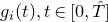 $g_i(t),t\in [0,\hat T]$
such that (1)–(4) hold for all
 $x\in B_{g_0}(x_0,1+\bar r_i)\times (0,\hat T]$
. By [Reference ChenChe09, Corollary 3.2] and [Reference Chow, Chu, Glickenstein, Guenther, Isenberg, Ivey, Knopf, Lu, Luo and NiCCG+08, Theorem 14.16],
 $g_i(t)$
sub-converges to a Ricci flow g(t) on
 $M\times [0,\hat T]$
in the local smooth topology as
 $i\to+\infty$
.
Remark 3.6. In the case
 $\bar r=+\infty$
, we only manage to control the small local curvature concentration in the suitable scale (see Proposition 2.3). In contrast with the bounded-curvature case, the small global curvature concentration is preserved under bounded-curvature Ricci flow. It is unclear to us whether there is any jumping phenomenon of the curvature concentration in the case that the curvature is initially unbounded.
4. Compactness of manifolds with bounded curvature concentration
In this section, we use the local-smoothing result from Theorem 1.1 to discuss the compactness of the space of compact manifolds with bounded curvature concentration, i.e., Theorem 1.3. We start with a simple observation that the collection of manifolds satisfying the assumptions in Theorem 1.3 is pre-compact with respect to the Gromov–Hausdorff topology.
Lemma 4.1. Suppose that (M,g) is a compact manifold such that:
-
(1) there exists
$C_s\gt0$
so that for all
$u\in W^{1,2}(M)$
, and
\begin{align*}\bigg(\int_M u^{{2n}/({n-2})}\,d\mathrm{vol}_{g} \!\bigg)^{\!({n-2})/{n}}\leq C_s\int_M (|\nabla u|^2+ u^2) \,d\mathrm{vol}_{g} ;\end{align*}
-
(2)
$\mathrm{diam}(M,g)\leq D_0$
.


Then there exists
 $v_1(n,C_s,D_0)\gt0$
such that for all
 $0\lt r\leq \mathrm{diam}(M,g)$
and
 $x\in M$
,
 \begin{align*}\mathrm{Vol}_g(B_g(x,r) )\geq v_1 r^n.\end{align*}
Proof. This follows from [Reference YeYe15, Lemma 6.1].
Lemma 4.2. The collection of compact manifolds satisfying (a), (b), and (d) in Theorem 1.3 is pre-compact in the Gromov–Hausdorff topology.
Proof. By Lemma 4.1 and Theorem 1.3(b), a manifold (M,g) in the collection is uniformly volume doubling. The conclusion then follows from Gromov’s compactness (see Theorem [Reference GromovGro99]).
The basic idea in proving the compactness without Ricci geometry is based on finding a local homeomorphism from an open ball around a regular point to an open ball in a smooth manifold. This is based on mollifying the initial metrics locally using Theorem 1.1 to a metric with regularity.
Proof of Theorem 1.3. We will use
 $g_{i,0}$
to denote
 $g_i$
, to emphasize that it is the initial metric whenever smoothing is used. We closely follow the argument in [Reference NakajimaNak88] with modifications using ideas from [Reference Simon and ToppingST21] and the new smoothing result, i.e., Theorem 1.1. It is more convenient to first obtain a convergent sequence in metric geometry. By Lemma 4.2, we may assume that
 $(M_i,g_{i,0})$
converges to a metric space
 $(X,d_\infty)$
in the Gromov–Hausdorff topology after passing to subsequence. We also let
 $\varphi_i: (M_i,d_{g_{i,0}})\to (X,d_\infty)$
be a sequence of
 $\varepsilon_i$
—Gromov–Hausdorff approximations for some
 $\varepsilon_i\to 0$
as
 $i\to+\infty$
.
We let
 $\delta_1(n,v_0,C_s)$
be the constant from Theorem 1.1. We define the singular set
 $\mathcal{S}_r$
of scale
 $r\gt0$
by
 \begin{align*} \mathcal{S}_r := \{ x\in X: \liminf_{i\to\infty} \|\mathrm{Rm}(g_{i,0})\|_{L^{n/2}(B_{g_{i,0}}(x_i,r))}\ge \delta_1 \text{ for any }x_i\in M_i \text{ such that } d_\infty(\varphi_i(x_i), x)\to 0 \}\end{align*}
and we consider
 \begin{align*} \mathcal{S}:=\bigcap_{r\gt0}\mathcal{S}_r.\end{align*}
Claim 4.3.
The set
 $\mathcal{S}$
is a finite set. That is,
 $\mathcal{S}=\{p_i\}_{i=1}^N$
for some
 $N\leq (2\Lambda_0\delta_1^{-1})^{n/2}$
. In particular,
 $\mathcal{S}$
is empty if
 $\Lambda_0\lt\delta_1/2$
.
Proof of Claim 4.3. For any fixed
 $r\gt0,$
we take a collection
 $\{x^j\}_{j\in J}\subseteq\mathcal{S}$
such that
 $\{B_{d_\infty}(x^j, 2r):j\in J\}$
is a disjoint collection of balls satisfying
 \begin{align*} \mathcal{S}\subseteq \bigcup_{j\in J} B_{d_\infty}(x^j, 3r).\end{align*}
For each
 $j\in J$
,
 $x^j\in \mathcal{S}_r$
for
 $r\gt0$
. We can find an approximating sequence
 $x^j_i\in M_i$
of
 $x^j$
such that
 $d_\infty(\varphi_i(x_i),x)\to 0$
and for large enough i, we have
 \begin{align*} \bigg(\int_{B_{g_i}(x^j_i,r)} |\mathrm{Rm}(g_{i,0})|^{n/2} d\mathrm{vol}_{g_{i,0}} \!\bigg)^{\!2/n} \gt \frac12\delta_1 .\end{align*}
By the disjoint property in X and the approximating property of
 $x^j_i$
’s, we know that for large i,
 $\{B_{g_i}(x_i^j, r):j\in J\}$
is a disjoint collection in
 $M_i.$
Hence, in particular, we derive
 \begin{align*} |J| \le (2\Lambda_0 \delta_1^{-1})^{n/2} ,\end{align*}
where
 $\Lambda_0$
is from the assumption of Theorem 1.3. This bound is independent of r and it particularly implies that
 \begin{align*} |\mathcal{S}|\le (2\Lambda_0 \delta_1^{-1})^{n/2}.\end{align*}
This proves the claim.
To show that the topological space M induced by
 $(X\setminus \mathcal{S},d_\infty)$
is in fact a manifold with bi-Hölder charts, we must show that given an arbitrary
 $x\in X\setminus\mathcal{S}$
, there is a neighborhood of x that is bi-Hölder homeomorphic to an open subset of a complete Riemannian manifold. We follow the treatment in [Reference Simon and ToppingST21].
Let
 $x\in X\setminus\mathcal{S}$
. Then there exist
 $r\gt0$
and
 $x_i\in M_i$
such that
 $d_\infty(\varphi_i(x_i),x)\to 0$
and
 \begin{align*}\|\mathrm{Rm}(g_{i,0})\|_{L^{n/2}(B_{g_{i,0}}(x_i,r))}\lt \delta_1\end{align*}
for large enough i. By considering
 $\tilde g_{i,0}:=(3r)^{-2}g_{i,0}$
, we might assume that
 $r=3$
. By Theorem 1.1 with
 $\bar r=0$
, there exists a Ricci flow
 $g_i(t)$
on
 $B_{g_{i,0}}(x_i,1)\times [0,\hat T]$
such that
 $g_i(0)=g_{i,0}$
and:
-
(1)
$|\mathrm{Rm}(g_i(t))|\leq \Lambda_1 \delta_1 t^{-1}$
; -
(2)
$\mathrm{inj}(g_i(t))\geq \sqrt{t}$
; -
(3)
$\|\mathrm{Rm}(g_i(t))\|_{L^{n/2}(B_{g_i(t)}(x_i,1/2))}\leq \Lambda_1 \varepsilon $
; and -
(4)
$\nu (B_{g_i(t)}(x_i,2L\sqrt{\hat T},g_i(t),L^2\hat T )\geq -\Lambda_1$




for all
 $(x,t)\in B_{g_{i,0}}(x_i,1)\times (0,\hat T]$
. Moreover, we might assume that for some
 $C_1(n,v_0,C_s)\gt0,\gamma(n,v_0,C_s)\in (0,1),$
we have
 \begin{align} C_1^{-1} (d_{g_i(t)}(x,y))^{1/\gamma}\leq d_{g_{i,0}}(x,y)\leq C_1 (d_{g_i(t)}(x,y))^{\gamma}\end{align}
for all
 $x,y\in B_{g_{i,0}}(x_i,1)$
and
 $t\in [0,\hat T]$
.
We now have all the necessary ingredients to carry out the proof in [Reference Simon and ToppingST21, Theorem 1.4 and Corollary 1.5]. We only give a sketch. We use Shi’s estimates and apply smooth compactness on
 $g_i(\hat T)$
to obtain a family of local diffeomorphisms
 $F_i$
such that
 $F_i^*g_i(t)$
sub-converges to
 $g_\infty(t)$
on
 $B_{g_\infty(\hat T)}(x_\infty,\sigma)$
for
 $\sigma\leq C_1^{-1}\sigma^{-\gamma}$
. Using
 $F_i$
, we might use the argument in the proof of [Reference Chan, Chen and LeeCCL22, Theorem 1.4] to show that
 $F_i^*d_{g_{i,0}}$
sub-converges to a distance function
 $\tilde d_\infty$
on
 $B_{g_\infty(\hat T)}(x_\infty,\sigma)$
that is locally bi-Hölder to the distance
 $d_{g_\infty(\hat T)}$
due to (4.1). The topological manifold structure in proximity to x follows from the uniqueness of the pointed Gromov–Hausdorff limits, which identifies
 $\tilde d_\infty$
in proximity to
 $x_\infty$
with
 $d_\infty$
in proximity to x.
Remark 4.4. From Claim 4.3, when
 $\Lambda_0$
is sufficiently small, then
 $\mathcal{S}$
is empty. In this case, from the proof of Theorem 1.3,
 $g_i(t)$
exists globally on
 $M_i\times[0,\hat T]$
. In particular, we can construct X by applying smooth compactness on
 $(M_i,g_i(\hat T))$
so that X admits a smooth structure.


5. Application to topological gap theorems
In this section, we will use Theorem 1.1 to prove the gap theorem in a differentiable structure of manifolds with small curvature concentration, i.e., Theorem 1.4. We start with the long-time existence. If the initial metric is assumed to have bounded curvature, this has been obtained earlier by [Reference Chau and MartensCM26a] (see also [Reference ChenChe22]).
Theorem 5.1.
For
 $n\geq 3$
and
 $C_s\gt0$
, there exist
 $\delta_0(n,C_s),\Lambda(n,C_s)\gt0$
such that if
 $(M^n,g_0)$
is a complete non-compact manifold satisfying Theorem 1.4(a)–(c), then there exists a unique complete Ricci flow g(t) on
 $M\times [0,+\infty)$
such that
 $g(0)=g_0$
and:
-
(i)
$|\mathrm{Rm}(g(t))|\leq \Lambda\varepsilon t^{-1}$
; -
(ii)
$\mathrm{inj}(g(t))\geq \sqrt{ t}$
; -
(iii)
$\|\mathrm{Rm}(g(t))\|_{L^{n/2}(M,g(t))}\leq \varepsilon$
; and -
(iv)
$\nu(M,g(t))\geq -\Lambda$
.


Furthermore, we have
 $\sup_M|\mathrm{Rm}(g(t))|=o(1)/t$
as
 $t\to +\infty$
.
Proof. By [Reference MartensMar25a, Lemma 3.3], the global entropy is bounded from below. By applying Theorem 3.5 on
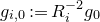 $g_{i,0}:=R_i^{-2}g_0$
for some
 $R_i\to+\infty$
and rescaling it back, we obtain a sequence of Ricci flows
 $g_i(t),t\in [0,R_i^2\hat T],$
satisfying the desired properties. By [Reference LeeLee25],
 $g_i(t)=g_{i+k}(t)$
for all
 $t\in [0, \hat T R_i] $
and
 $k\in \mathbb{N}$
. Thus, we obtain a long-time solution g(t) with (i), (ii), and (iv). It also satisfies a rough form of (iii) that the upper bound is
 $\Lambda \varepsilon$
. By Lemma 2.1, we recover the sharp upper bound
 $\varepsilon$
. The curvature estimate as
 $t\to +\infty$
follows from [Reference Chau and MartensCM26a, Theorem 1.2].
Remark 5.2. In contrast to the bounded-curvature case studied in [Reference Chau and MartensCM26a], we require volume growth to be at most Euclidean. It is unclear whether the volume-growth assumption is necessary.
Using Theorem 5.1, the diffeomorphic gap theorem is immediate from the existence of Ricci flow and its estimates.
Proof of Theorem 1.4. This follows from Theorem 5.1 and [Reference Huang and PengHP26, Theorem 1.1] (see also [Reference He and LeeHL21, Theorem 1.1] and [Reference WangWan20, Theorem 5.7]).
Basic examples of manifolds satisfying the assumptions in Theorem 1.4 are compact perturbations of Euclidean metrics. By the rigidity case in positive-mass theorems, we observe that the additional condition on scalar curvature
 $\mathcal{R}\geq 0$
is strong enough to rule them out. Motivated by this, we conjecture the following.
Conjecture 5.3. For any
 $C_s,v_0\gt0$
and
 $n\geq 3$
, there exists
 $\delta_0(n,C_s,v_0)\gt0$
such that the following holds. Suppose that
 $(M^n,g_0)$
is a complete non-compact manifold such that:
-
(a)
$C_{sob}(M)\geq C_s^{-1}$
; -
(b)
$\mathrm{Vol}_{g_0}(B_{g_0}(x,r))\leq v_0r^n$
for all
$(x,r)\in M\times \mathbb{R}_+$
; -
(c)
$\|\mathrm{Rm}(g_0)\|_{L^{n/2}(M)}\leq \delta_0(n,C_s,v_0)$
; and -
(d)
$\mathcal{R}(g_0)\geq 0$
.


Then
 $(M,g_0)$
is isometric to
 $\mathbb{R}^n$
.
Remark 5.4. When (d) is strengthened to
 $\operatorname{Ric}(g_0)\geq 0$
, the conjecture has been proved by Chan and the first-named author [Reference Chan and LeeCL24] (see also [Reference MartensMar25a]). This is based on using the long-time behavior of the Ricci flow to show that the tangent cone of M is isometric to Euclidean space and thus M must be Euclidean space by Colding’s volume continuity [Reference ColdingCol97]. Using the same circle of ideas, one should still be able to show that a tangent cone of M exists by [Reference Chan, Chen and LeeCCL22, Theorem 1.4] and that the blow-down of
 $(M,g_0)$
sub-converges to
 $\mathbb{R}^n$
in the
 $d_p$
-sense, introduced in [Reference Lee, Naber and NeumayerLNN23], using the method in [Reference Lee, Naber and NeumayerLNN23, Theorem 1.7]. It is, however, unclear how this asymptotic information constrains the original manifold M.
Acknowledgements
The authors would like to thank P.-Y. Chan for fruitful discussion.
Conflicts of interest
None.
Financial support
M-CL was supported by Hong Kong Research Grants Council (RGC) grant (Early Career Scheme) of Hong Kong no. 24304222 and no. 14300623, National Natural Science Foundation of China (NSFC) grant no. 12222122 and an Asian Young Scientist Fellowship. T-KL is grateful for the support from Bill Minicozzi through the National Science Foundation (NSF) Award DMS-2304684 and the support from the US Junior Oberwolfach Fellowship through the NSF Award DMS-2230648 while the project was carried out.
Journal information
Compositio Mathematica is owned by the Foundation Compositio Mathematica and published by the London Mathematical Society in partnership with Cambridge University Press. All surplus income from the publication of Compositio Mathematica is returned to mathematics and higher education through the charitable activities of the Foundation, the London Mathematical Society and Cambridge University Press.


 Open access

