
 L(S)
 L(S)
 γβ



%20--%3e%3c!DOCTYPE%20svg%20PUBLIC%20'-//W3C//DTD%20SVG%201.0//EN'%20'http://www.w3.org/TR/2001/REC-SVG-20010904/DTD/svg10.dtd'%3e%3csvg%20version='1.0'%20id='Layer_1'%20xmlns='http://www.w3.org/2000/svg'%20xmlns:xlink='http://www.w3.org/1999/xlink'%20x='0px'%20y='0px'%20width='64px'%20height='64px'%20viewBox='5.5%20-3.5%2064%2064'%20enable-background='new%205.5%20-3.5%2064%2064'%20xml:space='preserve'%3e%3cg%3e%3ccircle%20fill='%23FFFFFF'%20fill-opacity='0'%20cx='37.785'%20cy='28.501'%20r='28.836'/%3e%3cpath%20fill='%23595959'%20d='M37.441-3.5c8.951,0,16.572,3.125,22.857,9.372c3.008,3.009,5.295,6.448,6.857,10.314%20c1.561,3.867,2.344,7.971,2.344,12.314c0,4.381-0.773,8.486-2.314,12.313c-1.543,3.828-3.82,7.21-6.828,10.143%20c-3.123,3.085-6.666,5.448-10.629,7.086c-3.961,1.638-8.057,2.457-12.285,2.457s-8.276-0.808-12.143-2.429%20c-3.866-1.618-7.333-3.961-10.4-7.027c-3.067-3.066-5.4-6.524-7-10.372S5.5,32.767,5.5,28.5c0-4.229,0.809-8.295,2.428-12.2%20c1.619-3.905,3.972-7.4,7.057-10.486C21.08-0.394,28.565-3.5,37.441-3.5z%20M37.557,2.272c-7.314,0-13.467,2.553-18.458,7.657%20c-2.515,2.553-4.448,5.419-5.8,8.6c-1.354,3.181-2.029,6.505-2.029,9.972c0,3.429,0.675,6.734,2.029,9.913%20c1.353,3.183,3.285,6.021,5.8,8.516c2.514,2.496,5.351,4.399,8.515,5.715c3.161,1.314,6.476,1.971,9.943,1.971%20c3.428,0,6.75-0.665,9.973-1.999c3.219-1.335,6.121-3.257,8.713-5.771c4.99-4.876,7.484-10.99,7.484-18.344%20c0-3.543-0.648-6.895-1.943-10.057c-1.293-3.162-3.18-5.98-5.654-8.458C50.984,4.844,44.795,2.272,37.557,2.272z%20M37.156,23.187%20l-4.287,2.229c-0.458-0.951-1.019-1.619-1.685-2c-0.667-0.38-1.286-0.571-1.858-0.571c-2.856,0-4.286,1.885-4.286,5.657%20c0,1.714,0.362,3.084,1.085,4.113c0.724,1.029,1.791,1.544,3.201,1.544c1.867,0,3.181-0.915,3.944-2.743l3.942,2%20c-0.838,1.563-2,2.791-3.486,3.686c-1.484,0.896-3.123,1.343-4.914,1.343c-2.857,0-5.163-0.875-6.915-2.629%20c-1.752-1.752-2.628-4.19-2.628-7.313c0-3.048,0.886-5.466,2.657-7.257c1.771-1.79,4.009-2.686,6.715-2.686%20C32.604,18.558,35.441,20.101,37.156,23.187z%20M55.613,23.187l-4.229,2.229c-0.457-0.951-1.02-1.619-1.686-2%20c-0.668-0.38-1.307-0.571-1.914-0.571c-2.857,0-4.287,1.885-4.287,5.657c0,1.714,0.363,3.084,1.086,4.113%20c0.723,1.029,1.789,1.544,3.201,1.544c1.865,0,3.18-0.915,3.941-2.743l4,2c-0.875,1.563-2.057,2.791-3.541,3.686%20c-1.486,0.896-3.105,1.343-4.857,1.343c-2.896,0-5.209-0.875-6.941-2.629c-1.736-1.752-2.602-4.19-2.602-7.313%20c0-3.048,0.885-5.466,2.658-7.257c1.77-1.79,4.008-2.686,6.713-2.686C51.117,18.558,53.938,20.101,55.613,23.187z'/%3e%3c/g%3e%3c/svg%3e)
%20--%3e%3c!DOCTYPE%20svg%20PUBLIC%20'-//W3C//DTD%20SVG%201.0//EN'%20'http://www.w3.org/TR/2001/REC-SVG-20010904/DTD/svg10.dtd'%3e%3csvg%20version='1.0'%20id='Layer_1'%20xmlns='http://www.w3.org/2000/svg'%20xmlns:xlink='http://www.w3.org/1999/xlink'%20x='0px'%20y='0px'%20width='64px'%20height='64px'%20viewBox='5.5%20-3.5%2064%2064'%20enable-background='new%205.5%20-3.5%2064%2064'%20xml:space='preserve'%3e%3cg%3e%3ccircle%20fill='%23FFFFFF'%20fill-opacity='0'%20cx='37.637'%20cy='28.806'%20r='28.276'/%3e%3cg%3e%3cpath%20fill='%23595959'%20d='M37.443-3.5c8.988,0,16.57,3.085,22.742,9.257C66.393,11.967,69.5,19.548,69.5,28.5c0,8.991-3.049,16.476-9.145,22.456%20C53.879,57.319,46.242,60.5,37.443,60.5c-8.649,0-16.153-3.144-22.514-9.43C8.644,44.784,5.5,37.262,5.5,28.5%20c0-8.761,3.144-16.342,9.429-22.742C21.101-0.415,28.604-3.5,37.443-3.5z%20M37.557,2.272c-7.276,0-13.428,2.553-18.457,7.657%20c-5.22,5.334-7.829,11.525-7.829,18.572c0,7.086,2.59,13.22,7.77,18.398c5.181,5.182,11.352,7.771,18.514,7.771%20c7.123,0,13.334-2.607,18.629-7.828c5.029-4.838,7.543-10.952,7.543-18.343c0-7.276-2.553-13.465-7.656-18.571%20C50.967,4.824,44.795,2.272,37.557,2.272z%20M46.129,20.557v13.085h-3.656v15.542h-9.944V33.643h-3.656V20.557%20c0-0.572,0.2-1.057,0.599-1.457c0.401-0.399,0.887-0.6,1.457-0.6h13.144c0.533,0,1.01,0.2,1.428,0.6%20C45.918,19.5,46.129,19.986,46.129,20.557z%20M33.042,12.329c0-3.008,1.485-4.514,4.458-4.514s4.457,1.504,4.457,4.514%20c0,2.971-1.486,4.457-4.457,4.457S33.042,15.3,33.042,12.329z'/%3e%3c/g%3e%3c/g%3e%3c/svg%3e)
1. Introduction
In the recent paper [Reference Albin, Nesi and Palombaro1] the authors address the problem of finding solutions to a differential inclusion arising in the context of bounding the effective conductivity of a three-dimensional polycrystal [Reference Avellaneda, Cherkaev, Lurie and Milton2, Reference Nesi and Milton10, Reference Schulgasser12]. In the present follow-up paper, we focus on a certain property of the class of solutions described in the previous paper [Reference Albin, Nesi and Palombaro1], which is denoted by
 ${\mathcal L}(S)$
. We start by briefly describing the connection of
 ${\mathcal L}(S)$
with the so-called
 $G$
-closure of a polycrystalline conducting material, and then we will turn our attention to the differential inclusion that gives rise to
 ${\mathcal L}(S)$
. For a more detailed account of the polycrystal problem and its physical motivation we refer the reader to our previous paper [Reference Albin, Nesi and Palombaro1, § 2]. In the theory of composite materials, the set of all possible effective conductivities arising as a mixture of a single crystal with anisotropic conductivity
 $\sigma$
,
 \begin{equation} \sigma =\left ( \begin{array}{c@{\quad}c@{\quad}c} \sigma _1&0&0\\ 0&\sigma _2&0\\ 0&0&\sigma _3 \end{array} \right )\!,\quad 0\lt \sigma _3\leq \sigma _2\leq \sigma _1, \end{equation}
is known as the
 $G$
-closure and is commonly denoted by
 $G(\sigma )$
[Reference Avellaneda, Cherkaev, Lurie and Milton2, Reference Nesi and Milton10, Reference Milton7]. The characterization of
 $G(\sigma )$
is in general a difficult task and is still lacking in the present case. In two dimensions, the
 $G$
-closure for the polycrystal problem was understood long ago [Reference Dykhne3]. It is described in eigenvalue space as the following arc of hyperbola:
 \begin{equation*}\big\{(\sigma _1^*,\sigma _2^*)\in \mathbb{R}^2: \sigma _1^* \sigma _2^*=\sigma _1 \sigma _2, \,\sigma _2\leq \sigma _2^* \leq \sigma _2^*\leq \sigma _1\big\}.\end{equation*}
It has been established that partial knowledge of
 $\partial G(\sigma )$
can lead, in some cases, to the knowledge of larger parts of it. An interesting example is found in Ref. [Reference Milton and Nesi8] (for more details see pp. 204 and 645–647 of Ref. [Reference Milton7]). The underlying idea is based upon previous work done in Refs [Reference Francfort and Milton4] and [Reference Milton6]. The set
 ${\mathcal L}(S)$
constructed in our previous study [Reference Albin, Nesi and Palombaro1] (see in particular proposition 5.10 therein) provides a new portion of
 $\partial G(\sigma )$
in the case of distinct eigenvalues
 $\sigma _i$
’s. We remark that explicit examples of sets, which are stable under lamination but not stable under homogenization and correspond to effective properties of materials, are relatively difficult to find. A remarkable one can be found in the study of Milton [Reference Milton7] (see p. 690) where, using an idea from S˘verák [Reference Šverák13], the author exhibits a composite consisting of seven anisotropic phases with an effective elastic tensor that cannot be realized by laminations of the seven given phases. We also mention the very elegant construction by Grabovsky [Reference Grabovsky5] of a family of rotationally invariant, non-negative, and two-homogeneous rank-one convex functions that are not quasiconvex.
We now formulate the differential inclusion that defines the set
 ${\mathcal L}(S)$
and refer the reader to our previous work [Reference Albin, Nesi and Palombaro1, § 2] for the exact link with the polycrystal problem.
Let
 $\mathbb M^{3\times 3}_{\mathrm{sym}}$
denote the set of real, symmetric
 $3\times 3$
matrices and let
 $ S \in \mathbb M^{3\times 3}_{\mathrm{ sym}}$
be given by
 \begin{equation} S=\left ( \begin{array}{c@{\quad}c@{\quad}c} s_1&0&0\\ 0&s_2&0\\ 0&0&s_3 \end{array} \right ) \end{equation}
subject to the constraints
 \begin{equation} 0\lt s_1 \lt s_2\lt s_3,\quad s_1+s_2+s_3=1. \end{equation}
We define the set
 $K(S)\subset \mathbb M^{3\times 3}_{\mathrm{ sym}}$
as follows:
 \begin{equation} K(S) :=\{ \lambda R^t S R: \lambda \in \mathbb{R}, \, R\in SO(3) \}. \end{equation}
Notice that
 $K(S)$
is unbounded. Set
 $C=[0,1]^3$
and denote by
 $W_{C}^{1,2}(\mathbb R^3;\mathbb R^3)$
the space of vector fields in
 $W^{1,2}_{\mathrm{ loc}}(\mathbb R^3;\mathbb R^3)$
that are
 $C$
-periodic. We look for
 $A\in \ \mathbb M^{3\times 3}_{\mathrm{ sym}}$
such that the following differential inclusion admits solutions:
 \begin{equation} \nabla u\in K(S) \, \text{ a.e.}, \quad u-Ax \in W_{C}^{1,2}(\mathbb{R}^3; \mathbb{R}^3). \end{equation}
Solutions are understood in the approximate sense of the existence of sequences
 $\{u_j\}\subset W_{C,A}^{1,2}\equiv W_{C}^{1,2}(\mathbb{R}^3; \mathbb{R}^3)+ A x$
that are bounded in
 $W^{1,2}_{\text{loc}}(\mathbb{R}^3;\mathbb{R}^3)$
and such that
 $\{\nabla u_j\}$
is
 $L^2_{\text{loc}}$
-equi-integrable and
 \begin{equation*} {\mathrm{dist}} (\nabla u_j, K(S))\to 0 \text{ locally in measure}. \end{equation*}
We denote the set of all such
 $A$
’s as
 $K^{app}(S)$
and point out that
 $K^{app}(S)$
is related to the so-called 2-quasiconvex hull of
 $K(S)$
as defined by Yan [Reference Yan14], with
 $K^{app}(S)$
being a subset of it (see also the work of Zhang [Reference Zhang15] for a less restrictive definition of the 2-quasiconvex hull). The notation
 $K^{app}(S)$
is introduced by Müller [Reference Müller9], and it refers to ‘approximate solutions’ in the sense of differential inclusions. By definition of
 $K(S)$
,
 $K^{app}(S)$
is invariant under conjugation by any rotation, i.e., if
 $A\in K^{app}(S)$
then
 $ R^t A R \in K^{app}(S)$
for each
 $R\in SO(3)$
. Therefore, it suffices to characterize the eigenvalues of the elements of
 $K^{app}(S)$
, which can thus be identified with a subset of
 $\mathbb{R}^3$
. In fact, because of its original physical motivation [Reference Albin, Nesi and Palombaro1, § 2], we are interested in those elements of
 $K^{app}(S)$
whose eigenvalues lie in the interval
 $[s_1,s_3]$
. Moreover, as
 $K^{app}(S)$
is a cone, we may then focus on the specific section Tr
 $A=1$
. Denoting by
 ${\mathcal H}(S)$
the closed hexagon in
 $\mathbb{R}^3$
obtained as the convex hull of
 $(s_1,s_2,s_3)$
and all of its permutations, our goal becomes to characterize the following set:
 \begin{equation} K^*(S):= \left \{A\in K^{app}(S)\!: A\in {\mathcal H}(S) \right \}\!. \end{equation}
The exact characterization of
 $K^*(S)$
is currently an open problem. The main contribution of our previous work [Reference Albin, Nesi and Palombaro1] is an inner bound for
 $ K^*(S)$
, which is precisely the set
 ${\mathcal L}(S)$
and which improves all the bounds that were previously known [Reference Avellaneda, Cherkaev, Lurie and Milton2, Reference Nesi and Milton10, Reference Nesi11]. The goal of the present paper is to prove that
 ${\mathcal L}(S)$
enjoys the stability under lamination property (see definition 4.1). Such property would be naturally fulfilled if we knew that
 ${\mathcal L}(S)$
coincides with its 2-rank-one convex hull or with
 $ K^*(S)$
(see, e.g., [Reference Müller9, Reference Zhang15]). However, in the absence of such results, we prove it in proposition 4.7 using the very definition of stability. Our proofs are performed in the space of symmetric invariants rather than that of the eigenvalues. This feature is likely to be useful in different contexts where a given set enjoys the same invariance properties as
 $K^{app}(S)$
.
2. Preliminary definitions and results
The present section collects definitions and results from our previous work [Reference Albin, Nesi and Palombaro1] that will be used in the rest of the paper.
Definition 2.1.
We denote by
 $\mathcal D\subset \mathbb M^{3\times 3}_{\mathrm{ sym}}$
the set of positive definite diagonal matrices with unit trace and by
 $\mathcal D_{\mathrm{ d}}\subset \mathcal D$
its subset of matrices with distinct eigenvalues. The eigenvalues of a matrix
 $M\in \mathcal D$
are denoted by lower case letters
 $m_1,m_2$
, and
 $m_3$
and ordered as follows:
 \begin{equation} 0\lt m_1\leq m_2\leq m_3. \end{equation}
Note that
 $S \in \mathcal D_{\mathrm{ d}}$
, as its eigenvalues are distinct. In what follows
 $\mathbb{S}^2$
denotes the set of unit vectors in
 $\mathbb{R}^3$
.
Definition 2.2.
Let
 $F\in \mathcal D_{\mathrm{ d}}$
. The set
 $\mathcal T^{1}(F)$
is the set of all
 $G\in \mathcal D$
such that
 \begin{equation} \begin{array}{c@{\quad}c} \exists \,R\in SO(3), n\in \mathbb{S}^2, \lambda \in \mathbb R\backslash \{1\} : & R^tGR = \lambda \, F +(1-\lambda ) n\otimes n. \end{array} \end{equation}
Definition 2.3.
Assume that
 $F\in \mathcal D_d$
and
 $G\in \mathcal D$
. Set
 \begin{align*} & \alpha _- (F,G) :=\max \left (\frac {g_1}{f_2},\frac {g_2}{f_3}\right )\!, & \alpha _+ (F,G):= \min \left (\frac {g_1}{f_1},\frac {g_2}{f_2},\frac {g_3}{f_3}\right )\!,\\ &\beta _-(F,G):= \max \left (\frac {g_1}{f_1},\frac {g_2}{f_2},\frac {g_3}{f_3}\right )\!, &\beta _+(F,G):=\min \left (\frac {g_2}{f_1},\frac {g_3}{f_2}\right )\!, \\ & A_\alpha (F,G):=[\alpha _- (F,G), \alpha _+ (F,G)], & A_\beta (F,G):=[\beta _-(F,G), \beta _+(F,G)],\\ &A(F,G) :=(A_\alpha (F,G)\cup A_\beta (F,G))\setminus \{1\} \,. \end{align*}
The interior and the boundary of
 $A(F,G)$
are denoted by
 $\mathrm{Int} A(F,G)$
and
 $\partial A(F,G)$
, respectively, and we adopt the convention
 $[a,b] =\emptyset$
, if
 $a\gt b$
.
Remark 2.4. From the definition it follows that
 $\alpha _+(F,G)\leq 1\leq \beta _-(F,G)$
and that
 $\alpha _+(F,G)=\beta _-(F,G)=1$
if and only if
 $f_i=g_i$
for each
 $i=1,2,3$
. Hence, the set
 $A(F,G)$
is always the union of two disjoint, possibly empty, bounded intervals.
The next algebraic lemma clarifies when condition (2.2) holds.
Lemma 2.5.
Let
 $F\in \mathcal D_d$
,
 $G\in \mathcal D$
. If
 $G\in \mathcal T^1(F)$
, then
 $\lambda \in A(F,G)$
. Conversely, if
 $A(F,G) \neq \emptyset$
, then
 $G\in \mathcal T^1(F)$
and, in particular, for each
 $\lambda \in A(F,G)$
, the vector
 $n=(n_1,n_2,n_3)$
that satisfies (2.2) is determined, not uniquely, by the following equations:
 \begin{equation} \begin{array}{c@{\quad}c} \displaystyle { n_1^2(F,G,\lambda ):= \frac {(g_1 -\lambda f_1)(g_2 -\lambda f_1)(g_3 -\lambda f_1)}{\lambda ^2(1-\lambda ) (f_2 - f_1)(f_3 - f_1)}}, \\\\ \displaystyle {n_2^2(F,G,\lambda ) := \frac {(g_1 -\lambda f_2)(g_2 -\lambda f_2)(g_3 -\lambda f_2)}{\lambda ^2(1-\lambda ) (f_3 - f_2)(f_1 - f_2)}}, \\\\ \displaystyle {n_3^2(F,G,\lambda ):= \frac {(g_1 -\lambda f_3)(g_2 -\lambda f_3)(g_3 -\lambda f_3)}{\lambda ^2(1-\lambda ) (f_1 - f_3)(f_2 - f_3)} }. \end{array} \end{equation}
In particular
 $F\in \mathcal T^{1}(F)$
because
 \begin{equation*} A(F,F)=\left[\alpha _-(F,F),\frac {1}{\alpha _-(F,F)}\right ]\setminus \{1\} = \!\left [\max\! \left (\frac {s_1}{s_2}, \frac {s_2}{s_3}\right )\!, \min\! \left (\frac {s_2}{s_1}, \frac {s_3}{s_2}\right )\right ]\setminus \{1\}\neq \emptyset . \end{equation*}
Remark 2.6. In the previous paper [Reference Albin, Nesi and Palombaro1] a slightly weaker version of lemma 2.5 was established and the notation was slightly different. Specifically, in lemma 3.4 [Reference Albin, Nesi and Palombaro1], it is assumed that the eigenvalues of
 $F$
and
 $G$
satisfy, in addition,
 \begin{equation} f_1\leq g_1\leq g_2\leq g_3\leq f_3. \end{equation}
The proof of lemma 2.5 follows the lines of the proof of lemma 3.4 [Reference Albin, Nesi and Palombaro1] with the only difference given by the formulas of
 $\alpha _+(F,G)$
and
 $\beta _-(F,G)$
, which, in the case when (2.4) is satisfied, read as
 \begin{align*} \alpha _+ (F,G)= \min \left (\frac {g_2}{f_2},\frac {g_3}{f_3}\right )\!,\quad \beta _-(F,G)= \max \left (\frac {g_1}{f_1},\frac {g_2}{f_2}\right )\!. \end{align*}
Remark 2.7. The restriction that
 $F\in \mathcal D_d$
omits the class of rank-one connections that occur between special pairs of uniaxial
 $F$
and
 $G$
. We revisit this restriction in remark 3.6, where we show that these cases cannot improve the inner bound.
3. The set
 ${\mathcal L}(S)$

We recall the definition of the set
 ${\mathcal L}(S)$
, which provides an inner bound for the set
 $K^{*}(S)$
(see Ref. [Reference Albin, Nesi and Palombaro1, § 5] for more details). We start by introducing the uniaxial points
 $U_{\alpha }$
and
 $U_{\beta }$
and the rotations
 $R_\alpha$
and
 $R_\beta$
(see definition 3.1). We then define
 $\Gamma _{\alpha }$
and
 $\Gamma _{\beta }$
as the projection on
 ${\mathcal H}(S)$
of the rank-one segments connecting a specific multiple of
 $S$
to
 $R_\alpha ^t U_{\alpha }R_\alpha$
and
 $R_\beta ^t U_{\beta }R_\beta$
, respectively (definition 3.3). The set
 ${\mathcal L}(S)$
is finally defined as the subset of
 ${\mathcal H}(S)$
enclosed by
 $\Gamma _{\alpha }$
and
 $\Gamma _{\beta }$
and appropriately reflected and rotated copies of
 $\Gamma _{\alpha }$
and
 $\Gamma _{\beta }$
(see definitions 3.4, 3.5, and figure 1(a) and (b)).
Definition 3.1. Set
 \begin{equation} \begin{array}{c@{\quad}c} U_{\alpha }= \left ( \begin{array}{c@{\quad}c@{\quad}c} u_{\alpha }&0&0\\ 0&u_{\alpha }&0\\ 0&0&1-2 u_{\alpha } \end{array} \right )\!, \quad U_{\beta }= \left ( \begin{array}{c@{\quad}c@{\quad}c} 1-2 u_{\beta }&0&0\\ 0&u_{\beta }&0\\ 0&0&u_{\beta } \end{array} \right )\!, \end{array} \end{equation}
where
 $u_{\alpha }$
and
 $u_{\beta }$
are the smallest and largest root of
 \begin{equation} b(x):=6 s_2\,x^2+ x\,\big(s_1 s_3-3 s_2-4 s_2^2\big)+ 2 s_2^2 \end{equation}
respectively. Set
 \begin{equation} \begin{array}{lll} n_\alpha =\left ( \begin{array}{c} \cos \varphi _\alpha \\0\\ \sin \varphi _\alpha \end{array} \right )\!,\quad R_\alpha = \left ( \begin{array}{c@{\quad}c@{\quad}c} 0&-1&0\\ -\cos \theta _\alpha &0&\sin \theta _\alpha \\ -\sin \theta _\alpha &0&-\cos \theta _\alpha \end{array} \right )\!,\\\\ n_\beta =\left ( \begin{array}{c} \cos \varphi _\beta \\0\\ \sin \varphi _\beta \end{array} \right )\!,\quad R_\beta = \left ( \begin{array}{c@{\quad}c@{\quad}c} \cos \theta _\beta &0&-\sin \theta _\beta \\ \sin \theta _\beta &0&\cos \theta _\beta \\ 0&-1&0 \end{array} \right )\!, \end{array} \end{equation}
with
 \begin{equation} \begin{aligned} \cos (2\varphi _\alpha ) & =\frac {s_2(s_1+s_3)+u_\alpha (2 s_1 s_3-s_1-s_3)}{(s_3-s_1)(s_2-u_\alpha )}, \\ \cos (2\varphi _\beta ) & =\frac {s_2(s_1+s_3)+u_\beta (2 s_1 s_3-s_1-s_3)}{(s_3-s_1)(s_2-u_\beta )}, \end{aligned} \end{equation}
 \begin{equation} \begin{aligned} \\[-30pt] \cos (2 \theta _\alpha ) & =\frac {u_\alpha (s_3-s_1)+(u_\alpha -s_2) \cos (2 \varphi _\alpha )}{s_2(1-3 u_\alpha )}, \\ \cos (2 \theta _\beta ) & =-\frac {u_\beta (s_3-s_1)+(u_\beta -s_2) \cos (2 \varphi _\beta )}{s_2(1-3 u_\beta )}. \end{aligned} \end{equation}
The next proposition collects results from Ref. [Reference Albin, Nesi and Palombaro1] (see Ref. [Reference Albin, Nesi and Palombaro1, Proposition 5.3]), characterizing the matrices of
 $U_\alpha$
and
 $U_\beta$
as solutions of a specific matrix equation. Set
 \begin{equation} \alpha := \frac {u_{\alpha }}{s_2},\quad \beta := \frac {u_{\beta }}{s_2}. \end{equation}
Proposition 3.2.
Let
 $U_\alpha , U_\beta , R_\alpha , R_\beta , n_\alpha , n_\beta$
be defined by (3.1)–(3.3). Then
-
(i)
$u_\alpha$
and
$u_\beta$
satisfy
$ s_1\leq u_{\alpha }\lt \frac 1 3\lt u_{\beta }\leq s_3$
; -
(ii)
$ \alpha _-(S,U_{\alpha })=\alpha _+(S,U_{\alpha }) = \alpha ,\quad \beta _-(S,U_{\beta })= \beta _+(S,U_{\beta }) = \beta$
; -
(iii) the matrices
$U_\alpha$
and
$U_\beta$
are the unique solutions to
(3.7)
\begin{equation} R_\alpha ^t U_{\alpha }R_\alpha = \alpha S +(1-\alpha )\, n_\alpha \otimes n_\alpha , \end{equation}
(3.8)respectively.
\begin{equation} R_\beta ^t U_{\beta }R_\beta = \beta S +(1-\beta )\, n_\beta \otimes n_\beta , \end{equation}


The matrices
 $U_\alpha$
and
 $U_\beta$
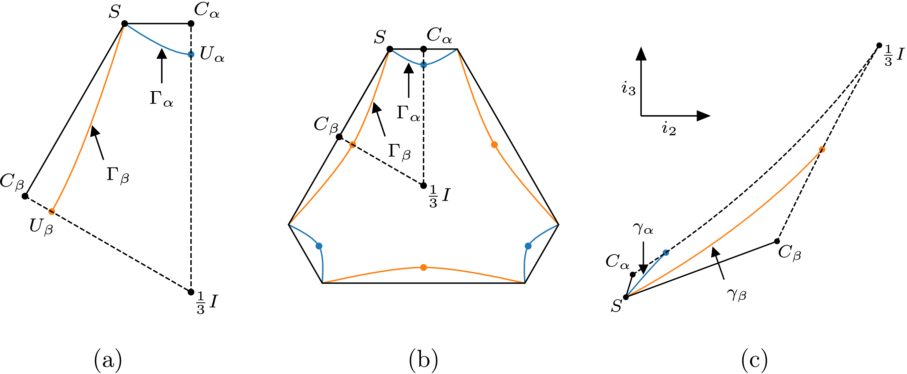
correspond to the blue and orange points in figure 1a. In order to define
 $\Gamma _\alpha$
and
 $\Gamma _\beta$
we will need an efficient way to describe curves in eigenvalue space. We therefore introduce some notation that will be used in § 4 as well. Let
 $F, G\in K^*(S)$
and assume that (2.2) holds. For each
 $\lambda \in A(F,G)$
and corresponding
 $n$
, see (2.3), consider the one-parameter family of unit-trace matrices:
 \begin{equation} \begin{array}{l}\displaystyle {M_{F,G}(\lambda ,t) =\eta (\lambda ,t) F+(1-\eta (\lambda ,t)) n\otimes n,\quad \eta (\lambda ,t):= \frac {\lambda }{\lambda + t(1-\lambda )}}, \end{array} \end{equation}
and note that
 \begin{equation*} M_{F,G}(\lambda ,0)=F,\quad M_{F,G}(\lambda ,1)=R^tGR. \end{equation*}
We now specialize (3.9) to the case when
 $F=S,$
and
 $\lambda =\alpha$
or
 $\lambda =\beta$
, see (3.6), and set
 \begin{equation} \begin{array}{l} M_\alpha (t):=M_{S,U_\alpha }(\alpha ,t),\quad M_\beta (t):=M_{S,U_\beta }(\beta ,t). \end{array} \end{equation}
We recall that
 \begin{equation} M_\alpha (1)=R_\alpha ^t U_\alpha R_\alpha ,\quad M_\beta (1)=R_\beta ^t U_\beta R_\beta . \end{equation}
Definition 3.3.
The curves
 $\Gamma _\alpha , \Gamma _\beta$
are defined as follows. Consider the parametric curves
 \begin{equation} t\mapsto m_\alpha (t):=(m_1(\alpha ,t),m_2(\alpha ,t),m_3(\alpha ,t)), \quad t\in [0,1], \end{equation}
 \begin{equation} t\mapsto m_\beta (t):=(m_1(\beta ,t),m_2(\beta ,t),m_3(\beta ,t)), \quad t\in [0,1], \end{equation}
where
 $ m_i(\alpha ,t), \, m_i(\beta ,t)$
denote the ordered eigenvalues of
 $M_\alpha (t)$
and
 $M_\beta (t)$
. Then
 \begin{equation*} \Gamma _{\alpha }:=m_\alpha ([0,1]),\quad \Gamma _{\beta }:=m_\beta ([0,1]). \end{equation*}
The curves
 $\Gamma _\alpha$
and
 $\Gamma _\beta$
are shown in figure 1a.
The left figure shows important fields in one sextant (
 $s_1\le s_2 \le s_3$
) of the unit-trace plane. The outer quadrilateral connects the field
 $S$
to the isotropic field
 $\frac {1}{3}I$
and the two uni-axial points,
 $C_{\alpha }=(\frac {s_1+s_2}{2},\frac {s_1+s_2}{2},s_3)$
and
 $C_{\beta }=(s_1,\frac {s_2+s_3}{2},\frac {s_2+s_3}{2})$
. The curves
 $\Gamma _{\alpha }$
and
 $\Gamma _{\beta }$
from definition 3.3 are also shown, together with their intersections with the uniaxial lines (the dashed lines). The centre figure shows the construction in definition 3.4. The set
 ${\mathcal L}(S)$
is enclosed by the union of the reflected copies of
 $\Gamma _\alpha$
and
 $\Gamma _\beta$
. The rightmost figure shows the fields in the sextant once again, but in the plane of the matrix invariants,
 $(i_2,i_3)$
, which are used in the proof of the stability. The curves
 $\gamma _\alpha$
and
 $\gamma _\beta$
, defined in (4.4), are the images of
 $\Gamma _\alpha$
and
 $\Gamma _\beta$
, respectively, when mapped to the matrix-invariants plane. Abusing notation we denote points by the same letters in (a)–(c).

Figure 1. Long description
Panel A: A diagram showing important fields in one sextant of the unit-trace plane. The outer quadrilateral connects the field to the isotropic field and the two uni-axial points, Cα and Cβ. The curves Γα and Γβ from definition 3.3 are also shown, together with their intersections with the uniaxial lines (the dashed lines). Panel B: A diagram showing the construction in definition 3.4. The set is enclosed by the union of the reflected copies of Γα and Γβ. Panel C: A diagram showing the fields in the sextant again, but in the plane of the matrix invariants, I2 and I3, which are used in the proof of the stability. The curves γα and γβ, defined in (4.4), are the images of Γα and Γβ, respectively, when mapped to the matrix-invariants plane.
Definition 3.4.
The closed curve
 $\Gamma$
is obtained as follows. First, reflect
 $\Gamma _{\alpha }$
along the line
 $m_1=m_2$
in the plane
 $m_1+m_2+m_3=1$
and then consider the union of the curves obtained with its
 $2\pi /3$
rotations within the unit trace plane. Next, reflect
 $\Gamma _{\beta }$
along the line
 $m_2=m_3$
in the plane
 $m_1+m_2+m_3=1$
and consider the union of the curves obtained with its
 $2\pi /3$
rotations within the unit trace plane. Finally,
 $\Gamma$
is the union of the six curves thus defined.
The construction of
 $\Gamma$
is shown in figure 1b. By construction,
 $\Gamma$
is a simple closed Jordan curve, and, for future reference, we note that
 \begin{equation} m_2(\alpha ,t) =s_2 \eta (\alpha ,t),\quad m_2(\beta ,t) =s_2 \eta (\beta ,t), \end{equation}
which readily follows from the fact that the second component of
 $n_\alpha$
and
 $n_\beta$
are zero.
Definition 3.5.
We denote by
 ${\mathcal L}(S)$
the bounded closed subset of
 ${\mathcal H}(S)$
enclosed by
 $\Gamma$
(see
figure 1b
).
Remark 3.6. In remark 2.7 we observed that lemma 2.5 cannot be applied if both
 $F$
and
 $G$
are uniaxial. One can easily check that in this case, at most one possible rank-one connection exists, and it requires
 $n$
to belong to the canonical basis and the double eigenvalue to be either the smallest for both matrices, or the largest for both matrices. These are well-known connections, already studied by Avellaneda et al. [Reference Avellaneda, Cherkaev, Lurie and Milton2]. In geometrical terms, the corresponding laminations can be visualized with the help of figure 1a, as segments lying either on the vertical dotted line or on the oblique dotted line. Thus, we can safely ignore them for the purposes of constructing
 $ {\mathcal L}(S)$
.
Theorem 3.7 ([Reference Albin, Nesi and Palombaro1], Theorem 5.7)
The set
 ${\mathcal L}(S)$
of definition 3.5 satisfies
 ${\mathcal L}(S)\subseteq K^*(S)$
.
4. Stability under lamination of the set
${\mathcal L}(S)$

We first recall the definition of stability under lamination for a subset of
 $K^*(S)$
. Then, in proposition 4.6, we provide an equivalent description in terms of geometrical quantities.
Definition 4.1.
We say that a subset
 $L$
of
 $K^*(S)$
is stable under lamination if the following holds. For any pair
 $F,G\in L$
such that
 ${\mathrm{rank}}(\lambda F- R^tGR$
) = 1 for some
 $\lambda \in \mathbb{R}$
and
 $R\in SO(3)$
, the projection on
 $K^*(S)$
of the rank-one segment connecting
 $\lambda F$
and
 $R^tGR$
belongs to
 $L$
. Equivalently, if
 $t\mapsto M_{F,G}(\lambda ,t)$
is defined by (3.9), then the curve
 $t\mapsto m_{F,G}(\lambda ,t)$
, with
 $m_{F,G}$
the triple of the corresponding ordered eigenvalues, satisfies
 $m_{F,G}(\lambda ,t) \in L$
for each
 $t\in [0,1]$
.
Recall that
 ${\mathcal H}(S)$
denotes the closed hexagon in
 $\mathbb{R}^3$
obtained as the convex hull of
 $(s_1,s_2,s_3)$
and all of its permutations.
Theorem 4.2.
The set
 ${\mathcal L}(S)$
is the smallest subset of
 ${\mathcal H}(S)$
containing its vertices that is stable under lamination.
Proof. The stability follows from propositions 4.6 and 4.7, while the fact that
 ${\mathcal L}(S)$
is the smallest subset follows from the work done in Ref. [Reference Albin, Nesi and Palombaro1].
Remark 4.3. The set
 $K^*(S)$
is stable under lamination (see, e.g., [Reference Müller9, Reference Zhang15]). As already observed in the introduction, we do not know whether
 ${\mathcal L}(S)=K^*(S)$
and therefore the proof of the stability of
 ${\mathcal L}(S)$
will require a careful examination of the rank-one connections between its points.
We find it convenient to change coordinates. Rather than using the eigenvalues
 $m_1,m_2,m_3$
, we use the symmetric invariants. The change of variable,
 \begin{equation*}(m_1,m_2,m_3)\mapsto (i_1,i_2,i_3):=(m_1+m_2+m_3,\, m_1 m_2+m_2 m_3+ m_3 m_1,\,m_1 m_2 m_3)\end{equation*}
is a diffeomorphism, except where two eigenvalues collapse. Recall that we work with symmetric matrices
 $M$
with unit trace, so that, for all of them
 $i_1(M)=1$
. Let
 $F\in \mathcal D_d$
and
 $G\in \mathcal D$
, then, using the notation in (3.9) we set
 \begin{align} & x(\lambda ,t,F,G):= i_2(M_{F,G}(\lambda ,t)),\quad y(\lambda ,t, F, G):= i_3(M_{F,G}(\lambda ,t)), \end{align}
 \begin{align} & \dot x(\lambda ,t,F,G)=\frac {\partial x}{\partial t}(\lambda ,t, F, G),\quad \dot y(\lambda ,t, F, G)=\frac {\partial y}{\partial t}(\lambda ,t, F, G), \end{align}
and,
 \begin{equation} x_F:=x(\lambda ,0,F,G),\!\quad x_G:=x(\lambda ,1,F,G),\!\quad y_F:=y(\lambda ,0,F,G),\!\quad y_G:=y(\lambda ,1,F,G). \end{equation}
See figure 1c for a plot of important fields in these coordinates. The curves
 $\Gamma _\alpha$
and
 $\Gamma _\beta$
will be denoted by
 $\gamma _{\alpha }$
and
 $ \gamma _{\beta }$
in the
 $(x,y)$
-space, as clarified by the following definition.
Definition 4.4.
For
 $M_\alpha$
and
 $M_\beta$
given by (3.10) and
 $t\in [0,1]$
, set
 \begin{equation*}\Phi _\alpha (t):=(i_2(M_\alpha (t)),i_3(M_\alpha (t))),\, \Phi _\beta (t):=(i_2(M_\beta (t)),i_3(M_\beta (t))).\end{equation*}
Then
 \begin{equation} \gamma _\alpha :=\Phi _\alpha ([0,1]),\quad \gamma _\beta :=\Phi _\beta ([0,1]). \end{equation}
Abusing notation, we identify points in matrix space with points in invariant space, so we can write
 $ M_\alpha (t)\in \gamma _{\alpha }$
. Similarly, the image of
 ${\mathcal L}(S)$
via the map
 $(i_2,i_3)$
is still denoted by
 ${\mathcal L}(S)$
.
The following lemma ensures that
 $\gamma _\alpha$
and
 $\gamma _\beta$
on the
 $(i_2,i_3)$
-plane are exactly as depicted in figure 1c. Its proof is postponed to § 7.2.
Lemma 4.5.
The sets
 $\gamma _\alpha$
and
 $\gamma _\beta$
are graphs of functions and intersect only at the point
 $(i_2(S),i_3(S))$
. At such a point the unit tangent vector to
 $\gamma _\alpha$
is obtained by a counterclockwise rotation by an angle of amplitude less than
 $\pi /2$
of the unit tangent vector to
 $\gamma _\beta$
.
Proposition 4.6.
The set
 ${\mathcal L}(S)$
given by definition 3.5 is stable under lamination if and only if the following geometrical property holds. Let
 $F, G$
both belong to either
 $\gamma _\alpha$
or
 $\gamma _\beta$
. Then the tangent vector at
 $F$
to any rank-one trajectory that starts at
 $F$
and ends at
 $G$
points strictly inwards
 ${\mathcal L}(S)$
, except for the optimal rank-one trajectory that lies exactly on
 $\gamma _\alpha$
or
 $\gamma _\beta$
.
Proof. The condition is clearly necessary. We focus on the sufficiency. Let
 $F,G\in {\mathcal L}(S)$
be such that
 ${\mathrm{rank}}(\lambda F- R^tGR) =1$
for some
 $\lambda \in \mathbb{R}$
and
 $R\in SO(3)$
. From now on we will drop the subscript
 $F,G$
from all the variables. Let
 $m(\lambda ,t)$
be as in definition 4.1 and assume by contradiction that the set
 $m(\lambda ,[0,1])$
intersects
 ${\mathcal L}(S)^c$
, the complement of
 ${\mathcal L}(S)$
. Because
 $m(\lambda ,t)$
may cross
 $\partial {\mathcal L}(S)$
only a finite number of times, say for
 $t=t_i, \, i=1,\ldots N$
, one can decompose the trajectory into a finite number of arcs
 $m(\lambda ,[t_{i-1},t_i])$
, each lying either inside
 ${\mathcal L}(S)$
or outside
 ${\mathcal L}(S)$
, except for its endpoints which lie exactly on
 $\partial {\mathcal L}(S)$
. In the first case there is nothing to prove. In the second case we observe that
 $m(\lambda ,t_{i-1})$
and
 $m(\lambda ,t_i)$
both belong to the same branch of
 $\partial {\mathcal L}(S)$
, namely,
 $m(\lambda ,t_{i-1}),m(\lambda ,t_{i})\in \gamma _{\alpha }$
or
 $m(\lambda ,t_{i-1}),m(\lambda ,t_{i})\in \gamma _{\beta }$
. This is a consequence of the bound
 $s_1\leq m_j\leq s_3$
for each
 $j=1,2,3$
and
 $t\in [0,1]$
. Then a necessary and sufficient condition for the arc starting at
 $m(\lambda ,t_{i-1})$
and ending at
 $m(\lambda ,t_i)$
to lie in
 ${\mathcal L}(S)$
is that the tangent vector at
 $m(\lambda ,t_{i-1})$
points inwards.
Using lemma 4.5, the geometric condition expressed in proposition 4.6, namely the condition for the tangent vector to point inwards, can be equivalently rephrased in terms of slopes of tangent vectors to certain rank-one trajectories, as stated in the next proposition.
Proposition 4.7.
If
 $F$
and
 $G$
belong to
 $\gamma _\alpha$
, with
 $F$
closer to
 $S$
, then the maximum of the slope of the tangent vector at
 $F$
among all the rank-one trajectories that start at
 $F$
and end at
 $G$
is attained when the trajectory is exactly the arc of
 $\gamma _\alpha$
joining
 $F$
and
 $G$
. When
 $F$
and
 $G$
belong to
 $\gamma _\beta$
, with
 $F$
closer to
 $S$
, then the trajectory that lies on
 $\gamma _\beta$
minimizes the slope among all possible rank-one trajectories connecting
 $F$
and
 $G$
.
Proof. It follows from propositions 5.4 and 7.1.
We conclude the present section by outlining the main steps towards the proof of the geometric conditions described in proposition 4.7, namely of propositions 5.4 and 7.1, on which theorem 4.2 is based.
STEP 1. Let
 $F\in \mathcal D_{\mathrm{ d}}$
and let
 $G\in {\mathcal T^{1}(F)}$
, see definition 2.2, so that the set
 $A(F,G)\neq \emptyset$
. For any
 $\lambda \in A(F,G)$
, consider the smooth trajectory originating at
 $F$
and ending at
 $G$
, see (3.9). Assuming
 $\dot {x}(\lambda ,0,F,G)\neq 0$
, define the ‘normalized slope’ in the invariants space as
 \begin{equation} \tau (\lambda ,F,G):=\left (\frac {\dot {y}(\lambda ,0,F,G)}{\dot {x}(\lambda ,0,F,G)}\right )\left (\frac {x_G}{y_G}\right )\!, \end{equation}
with
 $x_G$
and
 $y_G$
given by (4.1)–(4.3).
Remark 4.8. When
 $\dot {x}(\lambda ,0,F,G)\neq 0$
, the actual slope of the tangent vector at the initial point
 $F$
to the rank-one trajectory that starts at
 $F$
and ends at
 $G$
, namely
 $t\to (x(\lambda ,t,F,G),y(\lambda ,t,F,G))$
, is given by
 $\frac {\dot {y}(\lambda ,0,F,G)}{\dot {x}(\lambda ,0,F,G)}$
. With a slight abuse of notation, we use this terminology for
 $\tau (\lambda ,F,G)$
instead.
For
 $\dot {x}(\lambda ,0,F,G)\neq 0$
, we compute (4.5) obtaining the following:
 \begin{equation} \tau (\lambda ,F,G)= \displaystyle { \frac {1-\lambda ^2(3-2\lambda ) \frac {y_F}{y_G}}{\lambda \bigl (1-\lambda (2-\lambda ) \frac {x_F}{x_G}\bigr )} }, \end{equation}
see proposition 5.1.
STEP 2. Motivated by proposition 4.6, we specialize (4.6) to pairs
 $F,G$
that lie either on
 $\gamma _{\alpha }$
or
 $\gamma _{\beta }$
. We will proceed by considering in detail the case when
 $F,G$
lie on
 $\gamma _\alpha$
. We will hint at the necessary modifications for the case of
 $\gamma _\beta$
in § 7. Thus, we choose
 $F=M_{\alpha }(p)$
,
 $G=M_{\alpha }(q)$
, with
 $M_\alpha$
given by (3.10) and
 $0\leq p\leq q\leq 1, p\neq 1.$
We prove that,
 \begin{equation} 1-\lambda (2-\lambda ) \frac {x_{M_{\alpha }(p)}}{x_{M_{\alpha }(q)}}\neq 0, \quad \forall \, \lambda \in A(M_{\alpha }(p),M_{\alpha }(q)) \end{equation}
and
 \begin{equation} \tau (\lambda ,M_{\alpha }(p),M_{\alpha }(q))=h(\lambda ,p,q), \end{equation}
where
 $h$
is defined in (5.4) and depends only on the second eigenvalue
 $m_2(\alpha ,t)$
computed for
 $t=p$
and
 $t=q$
(3.14).
STEP 3. We prove that the slope is maximum when
 $\lambda = \alpha _+\big (M_{\alpha }(p),M_{\alpha }(q)\big )$
, namely, that for each
 $0\leq p\leq q\leq 1,\,p\neq 1$
one has
 \begin{equation} \max _{\lambda \in A(M_{\alpha }(p),M_{\alpha }(q))} h\left (\lambda ,p,q\right )= h(\alpha _+(M_{\alpha }(p),M_{\alpha }(q)),p,q). \end{equation}
This follows from proposition 5.4 and lemma 5.3, which imply that the slope on the right-hand side of (4.9) corresponds to the rank-one trajectory joining
 $M_{\alpha }(p)$
and
 $M_{\alpha }(q)$
that lies on
 $\gamma _{\alpha }$
. Notice that
 $x_{M_{\alpha }(q)}/y_{M_{\alpha }(q)}$
is positive; therefore, (4.9) is equivalent to maximizing the actual slope
 $\dot y/\dot x$
.
5. Proving steps 1–3
We now prove the three steps in order. The argument relies at a few key points on a technical computation, which we state and prove separately as lemma 6.1 in the next section. Deferring the lemma in this way keeps the present argument readable and establishes a context for the lemma.
5.1 Step 1: Proving ( 4.6 )
The next result gives a compact form for
 $\tau (\lambda ,F,G)$
. Recall definition 2.2.
Proposition 5.1.
Let
 $F\in \mathcal D_{\mathrm{ d}}$
and
 $G\in {\mathcal T^{1}(F)}$
. Then (4.6) holds for each
 $\lambda \in A(F,G)$
.
Proof. We use (6.2) of lemma 6.1 and for each
 $t\in [0,1]$
we compute
 \begin{equation} \begin{array}{ll} \dot {x}(\lambda ,t,F,G) &= \dfrac {\partial \eta }{\partial t}(\lambda ,t)\, \left (\dfrac {x_G-\lambda ^2x_F}{\lambda (1-\lambda )}-\dfrac {2(x_G-\lambda x_F)}{\lambda (1-\lambda )} \eta (\lambda ,t)\right ) \\\\ &=\dfrac {1}{\lambda ^2}\bigl (2(x_G-\lambda x_F) \,\eta ^3(\lambda ,t)- (x_G-\lambda ^2 x_F)\, \eta ^2(\lambda ,t)\bigr ) \\\\ \dot {y}(\lambda ,t,F,G) & = \,\dfrac {\partial \eta }{\partial t}(\lambda ,t)\,\left ( \dfrac {2(y_G-\lambda ^3y_F)}{\lambda ^2(1-\lambda )}\,\eta (\lambda ,t) - \dfrac {3(y_G-\lambda ^2y_F)}{\lambda ^2(1-\lambda )}\eta ^2(\lambda ,t)\right ) \\\\ &=\dfrac {1}{\lambda ^3}\bigl (3(y_G-\lambda ^2 y_F) \,\eta ^4(\lambda ,t)- 2(y_G-\lambda ^3 y_F)\, \eta ^3(\lambda ,t)\bigr ). \end{array} \end{equation}
Thus
 \begin{equation*} \dot {x}(\lambda ,0,F,G)= \frac {1}{\lambda ^2}(x_G - \lambda (2-\lambda ) x_F) ,\quad \dot y(\lambda ,0,F,G) = \frac {1}{\lambda ^3}\bigl (y_G - \lambda ^2(3-2\lambda )y_F\bigr ). \end{equation*}
In particular (4.6) holds when
 $\dot {x}(\lambda ,0,F,G)\neq 0$
.
5.2 Step 2: Proving ( 4.8 )
Consider the family
 $t\mapsto M_\alpha (t)$
and denote by
 $\mathcal E_j(t)$
the ordered eigenvalues of
 $M_\alpha (t)$
(see (3.12), (3.14)), namely
 \begin{equation} \mathcal E_j(t):=m_j(\alpha ,t). \end{equation}
Note that, by its very definition, the function
 $t\mapsto {\mathcal E}_2(t)$
is strictly decreasing. Define
 \begin{equation} \begin{array}{l} r(p,q):=\displaystyle {\frac {{\mathcal E}_2(p)}{{\mathcal E}_2(q)}\left (\frac {2u_\alpha - {\mathcal E}_2(p)}{2u_\alpha - {\mathcal E}_2(q)} \right )}, \quad s(p,q):=\displaystyle {\frac {{\mathcal E}_2^2(p)}{{\mathcal E}_2^2(q)}\left ( \frac {3u_\alpha - 2{\mathcal E}_2(p)}{3u_\alpha - 2 {\mathcal E}_2(q)}\right )} \end{array} \end{equation}
 \begin{equation} h(\lambda ,p,q):= \frac {1-\lambda ^2(3-2\lambda )\,s(p,q)}{\lambda (1-\lambda (2-\lambda )\,r(p,q))}. \end{equation}
The next result shows that
 $r$
,
 $s$
, and
 $h$
are well defined.
Proposition 5.2.
For each
 $0\leq p \leq q \leq 1,\,p\neq 1$
, and
 $\lambda \in A(M_{\alpha }(p),M_{\alpha }(q))$
, we have
 \begin{equation} 3u_\alpha -2 {\mathcal E}_2(q) \gt 0, \quad 1-\lambda (2-\lambda )r(p,q) \gt 0. \end{equation}
Proof. We show the first inequality in (5.5). Because
 $q\mapsto {\mathcal E}_2(q)\leq s_2$
, it is enough to check that
 $u_\alpha \gt \frac 2 3 s_2$
. To this end, we use the quadratic function
 $b$
defined in (3.2). We observe that
 $b(\frac 2 3 s_2)=\frac {2 s_1 s_2 s_3}{3}\gt 0$
and
 $b'(\frac 2 3 s_2)=-2s_1 s_2 -3s_2^2 -3s_2 s_3\lt 0$
, thus
 $\frac 2 3 s_2\lt u_\alpha$
, as
 $u_\alpha$
is the smallest root of the quadratic polynomial
 $b(x)$
.
We proceed to check the second inequality in (5.5). We distinguish two cases. If
 $p=q$
, then the statement is obvious. So we assume
 $p\lt q\leq 1$
. Because
 $\lambda \mapsto 1-\lambda (2-\lambda )\,r(p,q)$
is a quadratic polynomial in the variable
 $\lambda$
, it is minimized at
 $\lambda =1$
. Hence, it suffices to show that
 $1-\,r(p,q) \gt 0$
. By definition, this is the same as showing that
 \begin{equation*} ({\mathcal E}_2(p)-{\mathcal E}_2(q))({\mathcal E}_2(p)+{\mathcal E}_2(q)-2u_\alpha )\gt 0.\end{equation*}
Using the strict monotonicity of
 ${\mathcal E}_2$
, we obtain
 \begin{equation*} {\mathcal E}_2(p)-{\mathcal E}_2(q)\gt 0,\quad {\mathcal E}_2(p)+{\mathcal E}_2(q)-2u_\alpha \gt 2{\mathcal E}_2(1)-2u_\alpha =0. \end{equation*}
Formula (4.7) follows from (5.5) and (6.4) of lemma 6.1. Finally, (4.8) follows from (6.4) of lemma 6.1.
Set
 \begin{equation} \Lambda (p,q):=\frac {{\mathcal E}_2(q)}{{\mathcal E}_2(p)}, \end{equation}
and remark that
 $ \Lambda (p,q)\leq 1$
and
 $\Lambda (p,q)= 1$
if and only if
 $p=q$
. The next lemma implies that
 $ h(\Lambda (p,q),p,q)$
represents the slope of the tangent vector at the point
 $M_{\alpha }(p)$
when running a trajectory from
 $M_{\alpha }(p)$
to
 $M_{\alpha }(q)$
on the restriction of
 $\gamma _{\alpha }$
to the arc joining
 $M_{\alpha }(p)$
and
 $M_{\alpha }(q)$
. In addition, it gives an explicit formula for the extremes of the interval
 $A_\alpha (M_{\alpha }(p),M_{\alpha }(q))$
defined in (2.3).
Lemma 5.3.
Let
 $0\leq p \leq q \leq 1,\,p\neq 1$
and let
 $\Lambda (p,q)$
be defined in (5.6). There exist
 $R_p,R_q\in SO(3)$
such that
 \begin{equation} \begin{array}{c@{\quad}c} R_q^t M_{\alpha }(q) R_q = \Lambda (p,q) R_p^t M_{\alpha }(p) R_p+(1-\Lambda (p,q))n_\alpha \otimes n_\alpha . \end{array} \end{equation}
In particular
 $\Lambda (p,q)\in A(M_{\alpha }(p),M_{\alpha }(q))$
. Moreover
 \begin{equation} \alpha _-(M_{\alpha }(p),M_{\alpha }(q))=\max \left \{\frac { {\mathcal E_1(q)}}{{\mathcal E}_2(p)},\frac {{\mathcal E}_2(q)}{\mathcal E_3(p)}\right \}, \quad \alpha _+(M_{\alpha }(p),M_{\alpha }(q)) = \Lambda (p,q), \end{equation}
and
 \begin{equation} q\lt 1 \Longrightarrow \alpha _-(M_{\alpha }(p),M_{\alpha }(q))\lt \alpha _+(M_{\alpha }(p),M_{\alpha }(q)). \end{equation}
Proof. By definition of
 $\Gamma _{\alpha }$
, see (3.10), there exist two rotations
 $R_p$
and
 $ R_q$
such that
 \begin{equation} \left \{\begin{array}{c@{\quad}c} R_p^t M_{\alpha }(p) R_p = \eta (p) S+(1-\eta (p))n_\alpha \otimes n_\alpha \\\\ R_q^t M_{\alpha }(q) R_q = \eta (q) S+(1-\eta (q))n_\alpha \otimes n_\alpha , \end{array} \right . \end{equation}
where we set
 \begin{equation} \eta (t):= \eta (\alpha ,t), \end{equation}
with
 $\eta (\alpha ,t)$
defined in (3.9). Then, by eliminating
 $S$
from (5.10) and using (5.6), we deduce (5.7). The first equality in (5.8) holds by definition, as
 $p\neq 1$
implies that
 $M_\alpha (p)\in \mathcal D_d$
, and hence lemma 2.5 can be applied. We now prove the second equality in (5.8). Recall that by construction
 $\alpha _+\leq 1$
. If
 $p=q$
, the statement is immediate, as
 $\alpha _+(M_{\alpha }(p),M_{\alpha }(p)):=\min _{j}\left \{\frac {{\mathcal E}_j(p)}{{\mathcal E}_j(p)}\right \}=1=\Lambda (p,p)$
. Now let
 $p\lt q$
and recall that in this case
 $\alpha _+(M_\alpha (p),M_\alpha (q))\lt 1$
. By the monotonicity of
 $t\mapsto {\mathcal E}_2(t)$
, we have that
 $\Lambda (p,q)\lt 1$
and therefore, by the first part of the present lemma,
 $\Lambda (p,q) \in A_\alpha (M_\alpha (p),M_\alpha (q))\neq \emptyset$
, hence
 $\Lambda (p,q)\leq \max A_\alpha (M_\alpha (p),M_\alpha (q)) =: \alpha _+(M_\alpha (p),M_\alpha (q))$
. In contrast,
 \begin{equation*} \alpha _+(M_\alpha (p),M_\alpha (q)):=\min _{j}\left \{\frac {{\mathcal E}_j(q)}{{\mathcal E}_j(p)}\right \}\leq \frac {{\mathcal E}_2(q)}{{\mathcal E}_2(p)} =:\Lambda (p,q)\leq \alpha _+(M_\alpha (p),M_\alpha (q)) \,, \end{equation*}
which proves the second formula in (5.8). To prove (5.9) recall that
 $\alpha _-(M_\alpha (p),M_\alpha (q))\leq \alpha _+(M_\alpha (p),M_\alpha (q))$
, with equality if and only if for some
 $p$
and
 $q$
one has
 \begin{equation*} \hbox{either} \quad \frac {{\mathcal E}_1(q)}{{\mathcal E}_2(p)}=\frac {{\mathcal E}_2(q)}{{\mathcal E}_2(p)}\quad \hbox{or } \quad \frac {{\mathcal E}_2(q)}{{\mathcal E}_3(p)}=\frac {{\mathcal E}_2(q)}{{\mathcal E}_2(p)}\,. \end{equation*}
Hence, if equality occurs,
 $M_\alpha (p)$
or
 $M_\alpha (q)$
must be uniaxial. As
 $M_\alpha (p)$
and
 $M_\alpha (q)$
belong to the optimal trajectory
 $\gamma _{\alpha }$
, the only uniaxial point on
 $\gamma _{\alpha }$
is
 $U_{\alpha }$
, which corresponds to
 $q=1$
.
5.3 Step 3: Proving ( 4.9 )
We state the main result of the present section.
Proposition 5.4.
If
 $M_{\alpha }(p),M_{\alpha }(q)\in \gamma _{\alpha }$
, then for each
 $0\leq p \leq q \leq 1$
, with
 $p\neq 1$
,
 \begin{equation} \max _{\lambda \in A(M_{\alpha }(p),M_{\alpha }(q))} h(\lambda ,p,q)= h(\Lambda (p,q),p,q). \end{equation}
Proof. To ease notation we set, for
 $\lambda \gt 0$
,
 \begin{equation} \begin{array}{c@{\quad}c} c(\lambda ):= \lambda ^2(3-2\lambda ) ,& d(\lambda ):= \lambda (2-\lambda ), \end{array} \end{equation}
and write (5.4) as
 \begin{equation*} h(\lambda ,p,q)=\left (\frac 1 \lambda \right ) \frac {1- c(\lambda )\,s(p,q) }{1-d(\lambda )\,r(p,q)}. \end{equation*}
Formula (5.12) is equivalent to
 \begin{equation} h(\lambda ,p,q)\leq \left (\frac {1} {\Lambda (p,q)}\right ) \frac {1- c(\Lambda (p,q))\,s(p,q) }{1-d(\Lambda (p,q))\,r(p,q)}, \end{equation}
for each
 $0\leq p \leq q \leq 1$
, with
 $p\neq 1$
, and for each
 $\lambda \in A(M_{\alpha }(p), M_{\alpha }(q))$
. We now check that the right-hand side of (5.14) can be written as follows:
 \begin{equation} \begin{array}{c@{\quad}c} \displaystyle {\left (\frac {1}{\Lambda (p,q)}\right ) \frac {1- c(\Lambda (p,q))\,s(p,q) }{1-d(\Lambda (p,q))\,r(p,q)} = 3\left (\frac {{\mathcal E}_2(p)}{{\mathcal E}_2(q)}\right )\frac {2u_\alpha -{\mathcal E}_2(q)}{3u_\alpha -2{\mathcal E}_2(q)}}. \end{array} \end{equation}
Indeed, by the definition of
 $\Lambda$
(we will omit the dependence of
 $\Lambda$
upon
 $p$
and
 $q$
), the equation (5.15) is equivalent to
 \begin{equation} \begin{array}{c@{\quad}c} \displaystyle { \frac {1- c(\Lambda )\,s(p,q) }{1-d(\Lambda )\,r(p,q)} = 3\left (\frac {2u_\alpha -{\mathcal E}_2(q)}{3u_\alpha -2{\mathcal E}_2(q)}\right )}. \end{array} \end{equation}
Next, we use (6.3)–(6.4) to compute
 \begin{align*} 1- c(\Lambda )\,s(p,q)&=1-\Lambda ^2(3-2\Lambda )\frac {3 u_\alpha -2{\mathcal E}_2(p)}{3 u_\alpha -2{\mathcal E}_2(q)}\left (\frac {{\mathcal E}_2(p)}{{\mathcal E}_2(q)}\right )^2\\[3pt]&=1-(3-2\Lambda )\frac {3 u_\alpha -2{\mathcal E}_2(p)}{3 u_\alpha -2{\mathcal E}_2(q)}, \end{align*}
 \begin{equation*} 1- d(\Lambda )\,r(p,q)=1-\Lambda (2-\Lambda )\frac {2 u_\alpha -{\mathcal E}_2(p)}{2 u_\alpha -{\mathcal E}_2(q)}\left (\frac {{\mathcal E}_2(p)}{{\mathcal E}_2(q)}\right )=1-(2-\Lambda )\frac {2 u_\alpha -{\mathcal E}_2(p)}{2 u_\alpha -{\mathcal E}_2(q)}. \end{equation*}
Therefore, (5.16) is equivalent to
 \begin{align*} & (3 u_\alpha -2{\mathcal E}_2(q))-(3-2\Lambda )(3 u_\alpha -2{\mathcal E}_2(p))\\[3pt]&\quad -3(2 u_\alpha -{\mathcal E}_2(q))+3(2-\Lambda )(2 u_\alpha -{\mathcal E}_2(p))=0, \end{align*}
which follows by recalling that
 $\Lambda =\frac {{\mathcal E}_2(q)}{{\mathcal E}_2(p)}$
. Motivated by the previous calculation, we compute the left-hand side of (5.14), using the variable
 $X$
, with
 \begin{equation} X:= \lambda \frac {{\mathcal E}_2(p)}{{\mathcal E}_2(q)}=\frac {\lambda }{\Lambda (p,q)}. \end{equation}
We have
 \begin{equation*} \begin{array}{l} \!\!\!\!h(X \Lambda ,p,q) =\displaystyle { \frac {1-3 s(p,q)\Lambda ^2 X^2+2s(p,q)X^3 \Lambda ^3} {X \Lambda \big (1-2 r(p,q)\Lambda X+ r(p,q) \Lambda ^2 X^2\big )} }\\\\ =\displaystyle { \left (\frac {{\mathcal E}_2(p)}{{\mathcal E}_2(q)}\right )} \frac {1-3 X^2\left (\frac {3 u_\alpha -2{\mathcal E}_2(p)}{3 u_\alpha -2{\mathcal E}_2(q)}\right ) +2 X^3\left (\frac {{\mathcal E}_2(q)}{{\mathcal E}_2(p)}\right ) \left (\frac {3 u_\alpha -2{\mathcal E}_2(p)}{3 u_\alpha -2{\mathcal E}_2(q)}\right )}{X\left (1-2X \left (\frac {2 u_\alpha -{\mathcal E}_2(p)}{2 u_\alpha -{\mathcal E}_2(q)}\right )+X^2 \left (\frac {{\mathcal E}_2(q)}{{\mathcal E}_2(p)}\right ) \left (\frac {2 u_\alpha -{\mathcal E}_2(p)}{2 u_\alpha -{\mathcal E}_2(q)}\right )\right )} \\\\ =\displaystyle { \left (\frac {{\mathcal E}_2(p)}{{\mathcal E}_2(q)}\right )\left (\frac { 2u_\alpha -{\mathcal E}_2(q)}{3u_\alpha -2{\mathcal E}_2(q)}\right ) }\\\\ \displaystyle {\quad \times \frac {{\mathcal E}_2(p)(3 u_\alpha -2{\mathcal E}_2(q))-3X^2{\mathcal E}_2(p)(3 u_\alpha -2{\mathcal E}_2(p))+2X^3{\mathcal E}_2(q)(3 u_\alpha -2{\mathcal E}_2(p))}{X({\mathcal E}_2(p)(2 u_\alpha -{\mathcal E}_2(q))-2X {\mathcal E}_2(p)(2 u_\alpha -{\mathcal E}_2(p))+X^2{\mathcal E}_2(q)(2 u_\alpha -{\mathcal E}_2(p)))}}.\\\\ \end{array} \end{equation*}
Summarizing,
 \begin{equation} h\left (\lambda ,p,q\right )=h\left (\frac {{\mathcal E}_2(q)}{{\mathcal E}_2(p)}\,X,p,q\right )= \left (\frac {{\mathcal E}_2(p)}{{\mathcal E}_2(q)}\right )\left (\frac { 2u_\alpha -{\mathcal E}_2(q)}{3u_\alpha -2{\mathcal E}_2(q)}\right ) \frac {P(X)}{Q(X)}, \end{equation}
with
 \begin{equation*} \!\left \{\!\! \begin{array}{ll} P(X)={\mathcal E}_2(p) ( 3 u_\alpha -2 {\mathcal E}_2(q) )+3X^2 {\mathcal E}_2(p)(2{\mathcal E}_2(p) -3 u_\alpha )+ 2 X^3 {\mathcal E}_2(q) (3u_\alpha -2 {\mathcal E}_2(p) ),\\[4pt] Q(X)=X({\mathcal E}_2(p)(2u_\alpha -{\mathcal E}_2(q)) - 2 X {\mathcal E}_2(p)(2u_\alpha - {\mathcal E}_2(p)) + X^2{\mathcal E}_2(q)(2 u_\alpha -{\mathcal E}_2(p))). \end{array} \right . \end{equation*}
From (5.15) and proposition 5.2 we infer that
 $h(\Lambda (p,q),p,q)$
is positive. Therefore in order to prove (5.14) we only need to consider the case when
 $h(\lambda (p,q),p,q)$
is positive, which implies, by (5.18), that
 $\frac {P(X)}{Q(X)}$
is positive too. In order to proceed we first show that
 $Q\gt 0$
. As
 $X\gt 0$
by assumption, we need to prove that the quadratic polynomial in parentheses is positive, for
 $X\in [0,1]$
. Clearly, such polynomial is decreasing in
 $[0,1]$
; hence, it suffices to show that it is non-negative when
 $X=1$
. A straightforward calculation shows that
 \begin{equation*} Q(1)=2({\mathcal E}_2(p)-{\mathcal E}_2(q))({\mathcal E}_2(p)-u_\alpha ).\end{equation*}
The latter expression is non-negative by the strict monotonicity of
 $t\mapsto {\mathcal E}_2(t)$
. Next, we note that (5.14) holds if and only if
 \begin{equation*} \hbox{$3Q(X)-P(X) \ge q 0$ \quad for each \quad $\lambda \in A(M_{\alpha }(p), M_{\alpha }(q))$}.\end{equation*}
We compute
 $3Q(X)-P(X)$
and obtain
 \begin{equation*} 3Q(X)-P(X)= (1-X)^2 {\mathcal E}_2(p) \big (2 {\mathcal E}_2(q) +X {\mathcal E}_2(q)-3u_\alpha \big ), \end{equation*}
which shows that
 $X=1$
is in fact a double root and not merely a simple root. Therefore
 $3Q(X)-P(X)\geq 0$
if and only if for each
 $0\,\leq q\leq p\leq 1,\, p\neq 1$
and
 $\lambda \in A(M_{\alpha }(p), M_{\alpha }(q))$
 \begin{equation} \begin{array}{l} 2 {\mathcal E}_2(q)+ \lambda {\mathcal E}_2(p)-3 u_\alpha \geq 0. \end{array} \end{equation}
We now recall that
 $\min \{\lambda \in A(M_{\alpha }(p), M_{\alpha }(q))\}=\alpha _-(M_{\alpha }(p), M_{\alpha }(q))$
; hence, (5.19) holds if and only if for each
 $0\,\leq q\leq p\leq 1,\, p\neq 1$
 \begin{equation*} 2 {\mathcal E}_2(q)+ \alpha _-(M_{\alpha }(p),M_{\alpha }(q)) {\mathcal E}_2(p)-3u_\alpha \geq 0, \end{equation*}
which is in turn equivalent to
 \begin{equation} \alpha _-(M_{\alpha }(p),M_{\alpha }(q))+\frac {2{\mathcal E}_2(q)}{{\mathcal E}_2(p)}-\frac {3u_\alpha }{{\mathcal E}_2(p)}\geq 0. \end{equation}
We have thus proved that (5.14) is equivalent to (5.20), which we proceed to prove. For
 $p\neq 1$
, the matrix
 $M_\alpha (p)$
has distinct eigenvalues; hence, lemma 2.5 applies to the pair
 $(M_\alpha (p),M_\alpha (q))$
. By the definition of
 $\alpha _-(M_{\alpha }(p),M_{\alpha }(q))$
, (see (5.8)) we need to prove that
 \begin{equation*} \max \left \{\frac {{\mathcal E}_1(q)}{{\mathcal E}_2(p)}+\frac {2{\mathcal E}_2(q)}{{\mathcal E}_2(p)}- \frac {3u_{\alpha }}{{\mathcal E}_2(p)},\frac {{\mathcal E}_2(q)}{{\mathcal E}_3(p)}+\frac {2{\mathcal E}_2(q)}{{\mathcal E}_2(p)}- \frac {3u_{\alpha }}{{\mathcal E}_2(p)}\right \}\geq 0. \end{equation*}
It suffices to prove that the leftmost expression above is non-negative, namely that
 \begin{equation} \begin{array}{ll} K(q):={\mathcal E}_1(q) + 2{\mathcal E}_2(q)-3 u_{\alpha }\geq 0,\, \forall q\in [0,1], \end{array} \end{equation}
as
 ${\mathcal E}_2(p)$
is always strictly positive. We now regard
 $K$
as
 $K(q)=k(\eta (\alpha ,q))$
, where
 \begin{equation*} k(\eta ) := \lambda _{\min }(\eta S + (1-\eta )n_\alpha \otimes n_\alpha ) + 2s_2\eta - 3u_\alpha . \end{equation*}
The first term is the minimum eigenvalue of an affine family of real symmetric matrices and is, therefore, concave in
 $\eta$
by the standard argument that this function is the pointwise minimum of linear functionals. Thus, as the sum of a concave and an affine function,
 $k$
is also concave in
 $\eta$
. Therefore
 $k$
is minimized at the boundary of its domain of definition. As
 $q$
varies in the interval
 $[0,1]$
,
 $\eta (\alpha ,q)$
varies continuously in the interval
 $[\alpha ,1]$
. Thus,
 \begin{equation*}\min _{q\in [0,1]}K(q)=\min _{\eta \in [\alpha ,1]}k(\eta )=\min \{k( \alpha ), k(1)\}.\end{equation*}
We now verify that
 $\min \{k(\alpha ), k(1)\}=0$
. Note that
 \begin{equation*} \min \{k(\alpha ), k(1)\}=\min \{u_{\alpha }+2u_{\alpha }-3u_{\alpha }, s_1+2s_2-3u_{\alpha }\}=\min \{0,s_1+2s_2-3u_{\alpha }\}.\end{equation*}
It remains to show that
 $s_1+2s_2-3u_{\alpha }\geq 0$
. Recalling (3.2), one checks that
 \begin{equation*}b\left (\frac {s_1+2 s_2}{3}\right )=\frac {s_1(s_2-s_1)(s_2-s_3)}{3}\lt 0.\end{equation*}
Hence, the value
 $\frac {s_1+2s_2}{3}$
lies between the two roots of
 $b=0$
. In particular, it is greater than the smaller root, namely
 $u_{\alpha }$
, which is positive. Thus
 $\displaystyle {\min _{\eta \in [\alpha ,1]}k(\eta )=0}.$
Hence, (5.14) holds.
6. Computation of the invariants
We now establish the technical lemma used in the proof of propositions 5.1 and 5.2. Recall (3.9), (4.3), and (5.3) and define
 \begin{equation} x(t):=x(\alpha ,t,S,U_\alpha )=i_2(M_{\alpha }(t)),\quad y(t):=y(\alpha ,t,S,U_\alpha )=i_3(M_{\alpha }(t)). \end{equation}
Lemma 6.1.
Under the assumptions of proposition 5.1
, we have
 $\lambda \notin \{0,1\}$
and, for each
 $t\in [0,1]$
, one has
 \begin{equation} \left \{ \begin{array}{ll} x(\lambda , t, F,G)=\displaystyle { \frac {x_G-\lambda ^2 x_F}{\lambda (1-\lambda )}\,\eta (\lambda ,t)-\frac {x_G-\lambda x_F}{\lambda (1-\lambda )}\eta ^2(\lambda ,t)\,}\,\\\\ y(\lambda ,t,F,G)=\displaystyle {\frac {y_G-\lambda ^3 y_F}{\lambda ^2(1-\lambda )}\,\eta ^2(\lambda ,t) -\frac {y_G-\lambda ^2 y_F}{\lambda ^2(1-\lambda )}\,\eta ^3(\lambda ,t).} \end{array} \right . \end{equation}
In particular,
 \begin{equation} \begin{array}{lll} \left \{\begin{array}{l} x(t) =\displaystyle { \frac {2-3u_\alpha }{u_\alpha } \left (2u_\alpha -\mathcal E_2(t) \right )}{\mathcal E}_2(t) \\\\ y(t) =\displaystyle { \frac {1-2 u_\alpha }{u_\alpha }\left ( 3u_\alpha \, -2 \mathcal E_2(t)\right )\mathcal E_2^2(t)\,} , \end{array} \right . \end{array} \end{equation}
and, for any
 $0\leq p\leq q\leq 1$
, with
 $p\neq 1$
, we have
 \begin{equation} \begin{array}{c@{\quad}c} \displaystyle {\frac {x(p)}{x(q)}=r(p,q)},\quad & \displaystyle {\frac {y(p)}{y(q)}=s(p,q)}. \end{array} \end{equation}
Proof. The actual computation of the left-hand side of (6.2) shows that there are three functions that are constant along the trajectories. This motivates the following definitions. For
 $(\xi _1,\xi _2,\xi _3)\in \mathbb{R}^3$
, with
 $\xi _1\notin \{0,1\}$
, let
 \begin{equation*} \begin{array}{lll} \displaystyle { w_1(\xi _1,\xi _2,\xi _3):= \frac {\xi _3- \xi _1 \xi _2}{1-\xi _1 } }, & \displaystyle { w_2(\xi _1,\xi _2,\xi _3):= \frac {\xi _3- \xi _1^2 \xi _2}{\xi _1(1-\xi _1) } } ,& \displaystyle { w_3(\xi _1,\xi _2,\xi _3):= \frac {\xi _3- \xi _1^3 \xi _2}{\xi _1^2(1-\xi _1) } }. \end{array} \end{equation*}
We begin by showing that the functions
 $w_i$
are constant along the curves defined by the three homogeneous symmetric invariants
 $i_j$
. In other words, for each
 $t\in [0,1]$
, we prove that
 \begin{equation*} \left \{\begin{array}{l} \displaystyle { w_1(\eta (\lambda ,t),i_1(F), i_1(G))=w_1(\lambda ,i_1(F), i_1(G)) }, \\[8pt] \displaystyle { w_2(\eta (\lambda ,t),x_F,x_G)=w_2(\lambda ,x_F,x_G) },\quad \displaystyle { w_3(\eta (\lambda ,t),y_F,y_G)=w_3(\lambda ,y_F,y_G) }. \end{array} \right . \end{equation*}
Indeed, denoting by
 $f_j$
the eigenvalues of
 $F$
, we have
 \begin{equation} \begin{array}{c@{\quad}c} \det (M_{F,G}(\lambda ,t) -zI)\\ \\ =\displaystyle { \det (\eta (\lambda ,t) F - z I)+(1-\eta (\lambda ,t))\sum _{i=1}^{3} n_i^2(\eta (\lambda ,t) f_j - z)(\eta (\lambda ,t) f_k - z). } \end{array} \end{equation}
The last sum is taken with the convention that
 $i\neq j\neq k\neq i$
. As a function of the complex variable
 $z$
, equation (6.5) shows that a certain polynomial of degree three vanishes identically. Therefore, the coefficient of the polynomial on the left-hand side must be equal to those on the right-hand side. The coefficient of degree three is equal to −1 for both polynomials. We write the other three equalities. We have
 \begin{align} i_1(M(\lambda ,t)) &=\eta (\lambda ,t) i_1(F)+(1- \eta (\lambda ,t))\big[n_1^2+n_2^2+n_3^2\big]\nonumber \\[3pt] i_2(M(\lambda ,t)) &= \eta ^2(\lambda ,t) x_F+ \eta (\lambda ,t)(1- \eta (\lambda ,t))\nonumber \\[3pt] &\quad \times \big[n_1^2(f_2+f_3)+n_2^2(f_3+f_1)+n_3^2(f_1+f_2)\big]\nonumber \\[3pt] i_3(M(\lambda ,t))&= \eta ^3(\lambda ,t) y_F+ \eta ^2(\lambda ,t)(1- \eta (\lambda ,t)) \big[n_1^2f_2f_3+n_2^2f_3f_1+n_3^2f_1f_2\big]. \end{align}
Isolating the terms depending explicitly on the
 $n_i$
’s, one can see that the functions
 $w_j$
are independent of
 $t$
. Therefore, evaluating
 $w_j$
at
 $t=0$
we get
 \begin{equation} \left \{ \begin{array}{lll} n_1^2+n_2^2+n_3^2= \displaystyle { \frac {i_1(G)-\lambda i_1(F)}{1- \lambda }}, \\ n_1^2(f_2+f_3)+n_2^2(f_3+f_1)+n_3^2(f_1+f_2)=\displaystyle {\frac {x_G-\lambda ^2 x_F}{\lambda (1- \lambda )}}, \\ n_1^2f_2f_3+n_2^2f_3f_1+n_3^2f_1f_2=\displaystyle { \frac {y_G-\lambda ^3 y_F}{\lambda ^2(1- \lambda )}}. \end{array} \right . \end{equation}
Note that with our assumptions on
 $F$
and
 $G$
one has
 $\lambda \notin \{0,1\}$
, so the formulas in (6.7) make sense. Moreover, our assumptions imply that
 $i_1(M(\lambda ,t))=i_1(F)=1$
; thus, the first equation is automatically satisfied because
 $n$
has norm one. Plugging (6.6) into (6.7) we obtain
 \begin{equation*} x(\lambda , t, F,G)= \eta ^2(\lambda ,t) x_F+ \eta (\lambda ,t)\bigl (1-\eta (\lambda ,t)\bigr )w_2(\lambda ,x_F,x_G), \end{equation*}
which yields the first equation in (6.2). The derivation of the second one is similar and is thus omitted.
It remains to show (6.3) and (6.4). The latter follows from the former by very elementary algebraic manipulations which we omit. We focus on the first formula of (6.3). Specializing (6.2) to
 $F=S$
,
 $G=U_\alpha$
,
 $\lambda =\alpha$
, and recalling that
 ${\mathcal E}_2(t) = s_2\eta (t)$
, we find
 \begin{equation} \begin{array}{c} \displaystyle { x(\alpha ,t,S,U_\alpha ) = \frac {x_{U_\alpha }-\alpha ^2 x_S}{s_2\alpha (1-\alpha )}\,{\mathcal E}_2(t)-\frac {x_{U_\alpha }-\alpha x_S}{s_2^2\alpha (1-\alpha )}{\mathcal E}_2^2(t)}. \end{array} \end{equation}
Therefore, it is enough to prove that
 \begin{equation} \displaystyle { \frac {x_{U_\alpha }-\alpha ^2 x_S}{s_2\alpha (1-\alpha )}=2(2-3u_\alpha ), \quad \frac {x_{U_\alpha }-\alpha x_S}{s_2^2\alpha (1-\alpha )}=\frac {2 -3u_\alpha }{u_\alpha }. } \end{equation}
It is easy to check that the two equalities in (6.9) are equivalent to the following equation
 \begin{equation} 6s_2 u^2_\alpha +\big(x_S-4s_2-3s_2^2\big)u_\alpha +2s_2^2=0. \end{equation}
We now show that (6.10) is equivalent to
 $b(x)=0$
, where
 $b$
is the quadratic polynomial defined in (3.2), which holds by construction. Indeed,
 \begin{equation*} x_S-4s_2-3s_2^2=s_1s_3+s_2-s_2^2-4s_2-3s_2^2=s_1s_3-3s_2-4s_2^2. \end{equation*}
The proof of the second equation in (6.3) is similar and is omitted.
7. The
$\gamma _{\beta }$
-case and the proof of lemma 4.5

7.1
The
$\gamma _{\beta }$
-case

We will not treat the present case in detail, as the arguments are parallel to those used for the
 $\gamma _\alpha$
-case. Recall definitions 3.1 and 4.4 and denote the ordered eigenvalues of
 $M_{\beta }(t)$
by
 ${\mathcal F}_1(t)\leq {\mathcal F}_2(t)\leq {\mathcal F}_3(t)$
. Set
 \begin{equation*} \Lambda _\beta (p,q):= \frac {{\mathcal F}_2(q)}{{\mathcal F}_2(p)}, \qquad r_\beta (p,q):=\frac {{\mathcal F}_2(p)}{{\mathcal F}_2(q)}\left (\frac {2u_\beta - {\mathcal F}_2(p)}{2u_\beta - {\mathcal F}_2(q)}\right )\!. \end{equation*}
The following result is the analogue of (5.7) and of proposition 5.4.
Proposition 7.1.
Let
 $0\leq p \leq q \leq 1$
,
 $p\neq 1$
. There exist
 $R_p, R_q \in SO(3)$
such that
 \begin{equation*} \begin{array}{c@{\quad}c} R_q^t M_{\beta }(q) R_q = \Lambda _\beta (p,q) R_p^t M_{\beta }(p) R_p+(1-\Lambda _\beta (p,q))n_\beta \otimes n_\beta , \end{array} \end{equation*}
and
 \begin{equation} \min _{\lambda \in A(M_{\beta }(p),M_{\beta }(q))} h(\lambda ,p,q)= h(\Lambda _\beta (p,q),p,q). \end{equation}
The proof of proposition 7.1 is based on arguments that are very similar to those used to prove proposition 5.4 and is therefore omitted. We only point out that the minimization of
 $h$
in (7.1) is justified by lemma 4.5 (see proposition 4.7).
For completeness, in the next lemma we summarize the analogue of the results of proposition 5.2 and lemma 5.3.
Lemma 7.2.
For each
 $0\leq p \leq q\leq 1$
,
 $p\neq 1$
, and
 $\lambda \in A(M_{\beta }(p),M_{\beta }(q))$
, we have
 \begin{equation} 3u_\beta -2 {\mathcal F}_2(q) \gt 0, \quad 1-\lambda (2-\lambda )r_\beta (p,q) \gt 0, \end{equation}
 \begin{equation} \beta _-(M_\beta (p),M_\beta (q))=\Lambda _\beta (p,q),\quad {\displaystyle \beta _+(M_\beta (p),M_\beta (q))= \max \left \{\frac {{\mathcal F}_2(q)}{{\mathcal F}_1(p)},\frac { {{\mathcal F}_3(q)}}{{\mathcal F}_2(p)}\right \}}, \end{equation}
and
 \begin{equation} q\lt 1 \Longrightarrow \beta _-(M_\beta (p),M_\beta (q))\lt \beta _+(M_\beta (p),M_\beta (q)). \end{equation}
7.2 Proof of lemma 4.5
We add the subscript
 $\alpha$
in definition (6.1). Similarly we define
 \begin{equation*} x_\beta (t):=x(\beta ,t,S,U_\beta )=i_2(M_{\beta }(t)),\quad y_\beta (t):=y(\beta ,t,S,U_\beta )=i_3(M_{\beta }(t)). \end{equation*}
We use (6.3) to find
 \begin{equation*} \dot {x}_\alpha (t)= 2(2-3 u_\alpha )\Big (1-\frac {{\mathcal E}_2(t)}{u_\alpha }\Big )\dot {\mathcal E}_2(t) ,\quad \dot {y}_\alpha (t)= 6 (1-2 u_\alpha ) \Big (1-\frac {{\mathcal E}_2(t)}{u_\alpha }\Big ) {\mathcal E}_2(t) \dot {\mathcal E}_2(t). \end{equation*}
Similarly, from (6.2), we obtain
 \begin{equation*} \dot {x}_\beta (t)= 2(2-3 u_\beta )\Big (1-\frac {{\mathcal F}_2(t)}{u_\beta }\Big )\dot {\mathcal F}_2(t) ,\quad \dot {y}_\beta (t)= 6 (1-2 u_\beta ) \Big (1-\frac {{\mathcal F}_2(t)}{u_\beta }\Big ) {\mathcal F}_2(t) \dot {\mathcal F}_2(t). \end{equation*}
Taking into account (5.5) and (7.2), one can see that both
 $\dot {x}_\alpha (t)$
and
 $\dot {x}_\beta (t)$
are strictly positive for each
 $t\in (0,1)$
. Moreover, as
 ${\mathcal E}_2$
is strictly decreasing while
 ${\mathcal F}_2$
is strictly increasing,
 $\gamma _\alpha$
and
 $\gamma _\beta$
intersect only at the point
 $(i_2(S),i_3(S))$
. We now compute the slope of the tangent vectors at
 $(i_2(S),i_3(S))$
and find
 \begin{equation*} \frac {\dot y_\alpha (0)}{\dot x_\alpha (0)}=\frac {3 s_2(1-2 u_\alpha )}{2-3 u_\alpha },\quad \frac {\dot y_\beta (0)}{\dot x_\beta (0)}= \frac {3 s_2(1-2 u_\beta )}{2-3 u_\beta }. \end{equation*}
Finally,
 \begin{equation*} \frac {1-2 u_\alpha }{2-3 u_\alpha }\gt \frac {1-2 u_\beta }{2-3 u_\beta } \Longleftrightarrow u_\alpha \lt u_\beta , \end{equation*}
which follows from (i) of proposition 3.2.
Data availability
Data sharing is not applicable to this article as no datasets were generated or analysed during the current study.
Acknowledgements
V. Nesi gratefully acknowledges Progetti di Ricerca di Ateneo 2022, ‘Equazioni ellittiche e paraboliche non lineari’, rif. RM1221816BBB81FA e Progetto di Ateneo 2023, rif. RG123188B475BBF0, titolo ‘Singularities and interfaces: a variational approach to stationary and evolution problems.’ M. Palombaro is a member of the Gruppo Nazionale per l’Analisi Matematica, la Probabilità e le loro applicazioni (GNAMPA) of the Istituto Nazionale di Alta Matematica (INdAM).
Funding statement
This material is based upon work supported by the National Science Foundation under Grant No. 2108588 (N. Albin, Co-PI).
Competing interests
The authors have no conflicts of interest.

 s1≤s2≤s3
 S
 13I
 Cα=(s1+s22,s1+s22,s3)
 Cβ=(s1,s2+s32,s2+s32)
 Γα
 Γβ
 L(S)
 Γα
 Γβ
 (i2,i3)
 γα
 γβ
 Γα
 Γβ

 Open access

