1. Introduction
Viscous flow of passive and active suspensions in the presence of an infinite planar boundary is an important physical model in many areas of science and engineering. It serves as a useful paradigm for understanding the effect of confined geometries on the macroscopic flow behaviour of particulate flows, for example those of bacterial propulsion, cellular blood flow and colloidal suspensions (Kim & Karrila Reference Kim and Karrila1991; Cichocki & Jones Reference Cichocki and Jones1998; Bhattacharya & Bławzdziewicz Reference Bhattacharya and Bławzdziewicz2002; Veerapaneni et al. Reference Veerapaneni, Rahimian, Biros and Zorin2011; Spagnolie & Lauga Reference Spagnolie and Lauga2012). In problems where the Reynolds number is low, the ambient fluid is governed by the Stokes equations:
 $$\begin{eqnarray}{\it\mu}{\rm\Delta}\boldsymbol{u}(\boldsymbol{x})=\boldsymbol{{\rm\nabla}}p(\boldsymbol{x}),\quad \boldsymbol{{\rm\nabla}}\boldsymbol{\cdot }\boldsymbol{u}(\boldsymbol{x})=0,\end{eqnarray}$$
where
 ${\it\mu}$
is the fluid viscosity,
 $\boldsymbol{u}(\boldsymbol{x})=(u_{1}(\boldsymbol{x}),u_{2}(\boldsymbol{x}),u_{3}(\boldsymbol{x}))$
is the velocity of the fluid and
 $p(\boldsymbol{x})$
is the pressure. Assuming that the plane wall is located at
 $x_{3}=0$
and that the flow velocity decays in the far field,
 $$\begin{eqnarray}\displaystyle \boldsymbol{u}(\boldsymbol{x})\rightarrow 0\quad \text{as }|\boldsymbol{x}|\rightarrow \infty , & & \displaystyle\end{eqnarray}$$
the no-slip boundary condition is
 $$\begin{eqnarray}\boldsymbol{u}|_{x_{3}=0}=0.\end{eqnarray}$$
Boundary integral methods are particularly well suited for problems of this kind since they discretize the domain boundary alone (resulting in many fewer degrees of freedom) and impose the decay and the no-slip conditions exactly. Moreover, they avoid the need for artificial truncation of the computational domain and can be solved rapidly and with great accuracy using fast algorithms such as the fast-multipole method (FMM) and high-order accurate quadrature rules.
In order to reformulate the Stokes equations as a boundary integral equation, however, one needs to have access to the Green’s function for the half-space (Lorentz Reference Lorentz1896, Reference Lorentz1907; Lamb Reference Lamb1932; Happel & Brenner Reference Happel and Brenner1983). A now classical approach to constructing this Green’s function is due to Blake and others (Blake Reference Blake1971, Reference Blake1974; Blake & Chwang Reference Blake and Chwang1974; Aderogba & Blake Reference Aderogba and Blake1978a ,Reference Aderogba and Blake b ; Pozrikidis Reference Pozrikidis1992; Yu Reference Yu2003). Unfortunately, the resulting formulae are rather complicated, making them somewhat difficult to implement.
Here, we show that a much simpler alternative to the Blake solution can be obtained by combining a free-space image, which annihilates the tangential components of velocity, with a Papkovich–Neuber potential (Papkovich Reference Papkovich1932; Neuber Reference Neuber1934), which annihilates the normal component.
The present paper is organized as follows. We discuss Papkovich–Neuber potentials and the standard fundamental solutions for the Stokes equations in § 2 (see, for example, Lamb Reference Lamb1932; Happel & Brenner Reference Happel and Brenner1983; Kim & Karrila Reference Kim and Karrila1991; Pozrikidis Reference Pozrikidis1992). We also review Blake’s formula for the Stokeslet in a half-space. In § 3, we derive the image structures for Stokeslets, stresslets, rotlets and Stokes doublets.
In the appendices, we provide the analogous formulae for two-dimensional half-space Stokes kernels and for some problems of linear elasticity.
2. Fundamental solutions, the Papkovich–Neuber representation and Blake’s formulae
Before discussing the various standard fundamental solutions for the Stokes equations in free space, we introduce the Papkovich–Neuber representation, originally developed in Papkovich (Reference Papkovich1932) and Neuber (Reference Neuber1934) for problems of linear elasticity. Without loss of generality, we assume that the fluid viscosity
 ${\it\mu}=1$
in the rest of the paper.
Definition 2.1. Let
 ${\it\phi}(\boldsymbol{x}),\boldsymbol{x}\in \mathbb{R}^{3}$
, be a harmonic function. Then, the induced Papkovich–Neuber representation is defined to be the paired vector field
 $\boldsymbol{u}$
and scalar field
 $p$
given by
 $$\begin{eqnarray}\boldsymbol{u}(\boldsymbol{x})=x_{3}\boldsymbol{{\rm\nabla}}{\it\phi}(\boldsymbol{x})-\left[\begin{array}{@{}c@{}}0\\ 0\\ {\it\phi}(\boldsymbol{x})\end{array}\right],\quad p(\boldsymbol{x})=2\frac{\partial {\it\phi}(\boldsymbol{x})}{\partial x_{3}}.\end{eqnarray}$$
It is straightforward to verify that
 $(\boldsymbol{u},p)$
satisfy the Stokes equations (1.1).
Suppose now that a force vector
 $\boldsymbol{f}=(f_{1},f_{2},f_{3})$
is applied to a viscous fluid at a point
 $\boldsymbol{y}$
. Then, it is well known that the induced velocity and pressure can be computed using the Stokeslet (the single-layer kernel):
 $$\begin{eqnarray}\displaystyle & \displaystyle S_{ij}(\boldsymbol{x},\boldsymbol{y})=\frac{1}{8{\rm\pi}}\left[\frac{{\it\delta}_{ij}}{|\boldsymbol{x}-\boldsymbol{y}|}+\frac{(x_{i}-y_{i})(x_{j}-y_{j})}{|\boldsymbol{x}-\boldsymbol{y}|^{3}}\right],\quad i,j=1,2,3, & \displaystyle\end{eqnarray}$$
 $$\begin{eqnarray}\displaystyle & \displaystyle P_{j}(\boldsymbol{x},\boldsymbol{y})=\frac{1}{4{\rm\pi}}\frac{x_{j}-y_{j}}{|\boldsymbol{x}-\boldsymbol{y}|^{3}}, & \displaystyle\end{eqnarray}$$
 ${\it\delta}_{ij}$
is the Kronecker delta. More precisely, the velocity vector
 $\boldsymbol{u}(\boldsymbol{x})$
and pressure
 $p(\boldsymbol{x})$
are given by
 $$\begin{eqnarray}u_{i}(\boldsymbol{x})=\mathop{\sum }_{j=1}^{3}S_{ij}(\boldsymbol{x},\boldsymbol{y})f_{j},\quad p(\boldsymbol{x})=\mathop{\sum }_{j=1}^{3}P_{j}(\boldsymbol{x},\boldsymbol{y})f_{j}.\end{eqnarray}$$
The stresslet (or double-layer kernel) for the Stokes equations describes the velocity induced by an infinitesimal displacement
 $\boldsymbol{g}=(g_{1},g_{2},g_{3})$
(sometimes called the double-force source strength) at a point
 $\boldsymbol{y}$
with orientation vector
 ${\bf\nu}=({\it\nu}_{1},{\it\nu}_{2},{\it\nu}_{3})$
. It is given by
 $$\begin{eqnarray}\displaystyle & \displaystyle T_{ijk}(\boldsymbol{x},\boldsymbol{y})=\frac{3}{4{\rm\pi}}\frac{(x_{i}-y_{i})(x_{j}-y_{j})(x_{k}-y_{k})}{|\boldsymbol{x}-\boldsymbol{y}|^{5}},\quad i,j,k=1,2,3, & \displaystyle\end{eqnarray}$$
 $$\begin{eqnarray}\displaystyle & \displaystyle {\it\Pi}_{jk}(\boldsymbol{x},\boldsymbol{y})=\frac{1}{2{\rm\pi}}\left[-\frac{{\it\delta}_{jk}}{|\boldsymbol{x}-\boldsymbol{y}|^{3}}+\frac{3(x_{j}-y_{j})(x_{k}-y_{k})}{|\boldsymbol{x}-\boldsymbol{y}|^{5}}\right], & \displaystyle\end{eqnarray}$$
 $\boldsymbol{x}$
are
 $$\begin{eqnarray}u_{i}(\boldsymbol{x})=\mathop{\sum }_{j=1}^{3}\mathop{\sum }_{k=1}^{3}T_{ijk}(\boldsymbol{x},\boldsymbol{y}){\it\nu}_{k}g_{j},\quad p(\boldsymbol{x})=\mathop{\sum }_{j=1}^{3}\mathop{\sum }_{k=1}^{3}{\it\Pi}_{jk}(\boldsymbol{x},\boldsymbol{y}){\it\nu}_{k}g_{j}.\end{eqnarray}$$
2.1. Stokes flow in a half-space, Blake’s formula
Suppose now that a force vector
 $\boldsymbol{f}$
is applied to a viscous fluid in the upper half-space (
 $x_{3}>0$
). Then, the corresponding Stokeslet-induced velocity field fails to satisfy the no-slip condition (1.3). In order to annihilate the velocity field while satisfying the homogeneous Stokes equations in the upper half-space, Blake (Reference Blake1971) proposed the following image structure:
 $$\begin{eqnarray}S_{ij}^{W}(\boldsymbol{x},\boldsymbol{y})=S_{ij}(\boldsymbol{x},\boldsymbol{y})-S_{ij}(\boldsymbol{x},\boldsymbol{y}^{I})+2y_{3}^{2}S_{ij}^{D}(\boldsymbol{x},\boldsymbol{y}^{I})-2y_{3}S_{ij}^{SD}(\boldsymbol{x},\boldsymbol{y}^{I}),\end{eqnarray}$$
where
 $\boldsymbol{y}^{I}=(y_{1},y_{2},-y_{3})$
is the reflected image location. Here,
 $S^{D}$
is a modified source doublet, given by
 $$\begin{eqnarray}S_{ij}^{D}(\boldsymbol{x},\boldsymbol{y})=\frac{1}{8{\rm\pi}}(1-2{\it\delta}_{j3})\frac{\partial }{\partial x_{j}}\frac{x_{i}-y_{i}}{|\boldsymbol{x}-\boldsymbol{y}|^{3}},\end{eqnarray}$$
and
 $S^{SD}$
is a modified Stokes doublet, given by
 $$\begin{eqnarray}S_{ij}^{SD}(\boldsymbol{x},\boldsymbol{y})=(1-2{\it\delta}_{j3})\frac{\partial S_{i3}(\boldsymbol{x},\boldsymbol{y})}{\partial x_{j}}.\end{eqnarray}$$
Similar, but more involved, decompositions for the Stokes doublet and stresslet in a half-space are given in Blake & Chwang (Reference Blake and Chwang1974) and Pozrikidis (Reference Pozrikidis1992). It should be noted that the computation of the modified source doublet
 $S_{ij}^{D}$
requires the evaluation of three distinct harmonic dipole fields.
3. A new image formula
In this section, we derive a simpler image structure, using the Papkovich–Neuber representation which involves only a single harmonic function. Here,
 $\boldsymbol{y}^{I}$
, as above, will denote the image location
 $(y_{1},y_{2},-y_{3})$
. Now, however, we define reflected single-force, double-force and double-force-orientation vectors by negating their third components:
 $$\begin{eqnarray}\boldsymbol{f}^{I}=(f_{1},f_{2},-f_{3}),\quad \boldsymbol{g}^{I}=(g_{1},g_{2},-g_{3}),\quad {\bf\nu}^{I}=({\it\nu}_{1},{\it\nu}_{2},-{\it\nu}_{3}).\end{eqnarray}$$
We also make use of the harmonic potential due to a unit strength charge,
 $$\begin{eqnarray}G^{S}(\boldsymbol{x},\boldsymbol{y})=\frac{1}{4{\rm\pi}|\boldsymbol{x}-\boldsymbol{y}|},\end{eqnarray}$$
the harmonic potential due to a unit strength dipole with orientation vector
 ${\bf\nu}$
,
 $$\begin{eqnarray}G^{D}[{\bf\nu}](\boldsymbol{x},\boldsymbol{y})=\mathop{\sum }_{i=1}^{3}{\it\nu}_{i}\frac{\partial }{\partial y_{i}}\frac{1}{4{\rm\pi}|\boldsymbol{x}-\boldsymbol{y}|},\end{eqnarray}$$
and the harmonic potential due to a unit strength quadrupole with orientation vectors
 ${\bf\nu}$
and
 ${\bf\kappa}$
,
 $$\begin{eqnarray}G^{Q}[{\bf\nu},{\bf\kappa}](\boldsymbol{x},\boldsymbol{y})=\mathop{\sum }_{i=1}^{3}\mathop{\sum }_{j=1}^{3}{\it\nu}_{i}{\it\kappa}_{j}\frac{\partial ^{2}}{\partial y_{i}\partial y_{j}}\frac{1}{4{\rm\pi}|\boldsymbol{x}-\boldsymbol{y}|}.\end{eqnarray}$$
Finally, we recall that, through the Papkovich–Neuber representation (2.1), the harmonic function
 ${\it\phi}(\boldsymbol{x})$
induces velocity and pressure fields that can be written in component form as
 $$\begin{eqnarray}u_{i}(\boldsymbol{x})=x_{3}\frac{\partial }{\partial x_{i}}{\it\phi}(\boldsymbol{x})-{\it\delta}_{i3}{\it\phi}(\boldsymbol{x}),\quad p(\boldsymbol{x})=2\frac{\partial }{\partial x_{3}}{\it\phi}(\boldsymbol{x}).\end{eqnarray}$$
Of particular note is the fact that at
 $x_{3}=0$
, the only non-zero velocity component is
 $$\begin{eqnarray}u_{3}(\boldsymbol{x})=-{\it\phi}(\boldsymbol{x}).\end{eqnarray}$$
This suggests a simple two-step strategy. First, annihilate the tangential components of the velocity field induced by a Stokeslet (single-layer) or stresslet (double-layer) kernel. It is easy to see that this can be accomplished by subtracting the influence of a reflected single force
 $\boldsymbol{f}^{I}=(f_{1},f_{2},-f_{3})$
or double force
 $\boldsymbol{g}^{I}=(g_{1},g_{2},-g_{3}),{\bf\nu}^{I}=({\it\nu}_{1},{\it\nu}_{2},-{\it\nu}_{3})$
located at the image point
 $\boldsymbol{y}^{I}$
respectively. It remains only to match the remaining non-zero normal component
 $u_{3}$
, which we will do by a judicious choice of the Papkovich–Neuber potential
 ${\it\phi}(\boldsymbol{x})$
.
3.1. The Stokeslet correction
Following the discussion above, let us write out in more detail the velocity field
 $\boldsymbol{v}$
remaining after subtracting the image Stokeslet at
 $\boldsymbol{y}^{I}$
from the original Stokeslet at
 $\boldsymbol{y}$
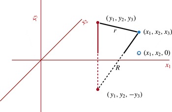
(figure 1):
 $$\begin{eqnarray}\displaystyle v_{i}(\boldsymbol{x})=\mathop{\sum }_{j=1}^{3}(S_{ij}(\boldsymbol{x},\boldsymbol{y})f_{j}-S_{ij}(\boldsymbol{x},\boldsymbol{y}^{I})f_{j}^{I}). & & \displaystyle\end{eqnarray}$$
At the interface
 $x_{3}=0$
, a straightforward computation yields
 $$\begin{eqnarray}v_{1}(\boldsymbol{x})=0,\quad v_{2}(\boldsymbol{x})=0,\quad v_{3}(\boldsymbol{x})=-\frac{f_{3}^{I}}{4{\rm\pi}}\frac{1}{|\boldsymbol{x}-\boldsymbol{y}^{I}|}-\frac{y_{3}}{4{\rm\pi}}\mathop{\sum }_{j=1}^{3}\frac{x_{j}-y_{j}^{I}}{|\boldsymbol{x}-\boldsymbol{y}^{I}|^{3}}f_{j}^{I}.\end{eqnarray}$$
The original source location is in the upper half-space at
 $(y_{1},y_{2},y_{3})$
and the reflected image source is at
 $(y_{1},y_{2},-y_{3})$
. For target points
 $(x_{1},x_{2},0)$
that lie on the half-space boundary, the distances
 $r$
and
 $R$
from the source and image are the same, simplifying the computation of
 $\boldsymbol{v}$
in (3.8).

By inspection of (3.8), it is clear that the harmonic potential
 ${\it\phi}$
required to cancel the non-zero normal component
 $v_{3}$
at the interface is that induced by a charge of strength
 $f_{3}^{I}$
and a dipole with orientation vector
 $\boldsymbol{f}^{I}$
of strength
 $y_{3}$
located at
 $\boldsymbol{y}^{I}$
. Thus, the velocity field
 $\boldsymbol{u}^{W}$
satisfying the desired no-slip boundary condition (1.3) can be expressed as
 $$\begin{eqnarray}u_{i}^{W}(\boldsymbol{x})=u_{i}^{A}(\boldsymbol{x})-u_{i}^{B}(\boldsymbol{x})-u_{i}^{C}(\boldsymbol{x}),\end{eqnarray}$$
where
 $\boldsymbol{u}^{A}$
and
 $\boldsymbol{u}^{B}$
are the velocity fields induced by the original free-space Stokeslet and the reflected image force vector respectively:
 $$\begin{eqnarray}u_{i}^{A}(\boldsymbol{x})=\mathop{\sum }_{j=1}^{3}S_{ij}(\boldsymbol{x},\boldsymbol{y})f_{j},\quad u_{i}^{B}(\boldsymbol{x})=\mathop{\sum }_{j=1}^{3}S_{ij}(\boldsymbol{x},\boldsymbol{y}^{I})f_{j}^{I}.\end{eqnarray}$$
Here,
 $u_{i}^{C}$
is the Papkovich–Neuber correction,
 $$\begin{eqnarray}u_{i}^{C}(\boldsymbol{x})=x_{3}\frac{\partial }{\partial x_{i}}{\it\phi}(\boldsymbol{x})-{\it\delta}_{i3}{\it\phi}(\boldsymbol{x}),\end{eqnarray}$$
where the harmonic potential
 ${\it\phi}$
is that due to a simple charge and dipole, both located at
 $\boldsymbol{y}^{I}$
:
 $$\begin{eqnarray}{\it\phi}(\boldsymbol{x})=f_{3}^{I}G^{S}(\boldsymbol{x},\boldsymbol{y}^{I})+y_{3}G^{D}[\boldsymbol{f}^{I}](\boldsymbol{x},\boldsymbol{y}^{I}).\end{eqnarray}$$
3.2. The stresslet correction
We state the image structure for the stresslet (the double-layer kernel) in the form of a theorem.
Theorem 1. Let a double force
 $\boldsymbol{g}$
with orientation vector
 ${\bf\nu}$
be located at
 $\boldsymbol{y}$
, resulting in the free-space velocity field
 $$\begin{eqnarray}\displaystyle u_{i}^{T}(\boldsymbol{x})=\mathop{\sum }_{j=1}^{3}\mathop{\sum }_{k=1}^{3}T_{ijk}(\boldsymbol{x},\boldsymbol{y}){\it\nu}_{k}g_{j}. & & \displaystyle\end{eqnarray}$$
Then, the corresponding velocity satisfying the no-slip boundary condition (1.3) is given by
 $$\begin{eqnarray}u_{i}^{T,W}(\boldsymbol{x})=\mathop{\sum }_{j=1}^{3}\mathop{\sum }_{k=1}^{3}T_{ijk}(\boldsymbol{x},\boldsymbol{y}){\it\nu}_{k}g_{j}-\mathop{\sum }_{j=1}^{3}\mathop{\sum }_{k=1}^{3}T_{ijk}(\boldsymbol{x},\boldsymbol{y}^{I}){\it\nu}_{k}^{I}g_{j}^{I}-\left[x_{3}\frac{\partial }{\partial x_{i}}{\it\phi}^{T}(\boldsymbol{x})-{\it\delta}_{i3}{\it\phi}^{T}(\boldsymbol{x})\right],\end{eqnarray}$$
where
 $$\begin{eqnarray}{\it\phi}^{T}(\boldsymbol{x})=2({\bf\nu}^{I}\boldsymbol{\cdot }\boldsymbol{g}^{I})G^{D}[\boldsymbol{h}](\boldsymbol{x},\boldsymbol{y}^{I})+2y_{3}G^{Q}[{\bf\nu}^{I},\boldsymbol{g}^{I}](\boldsymbol{x},\boldsymbol{y}^{I}),\end{eqnarray}$$
with
 $\boldsymbol{h}=(0,0,1)$
.
Proof. It should be noted first that the symmetric part of the Stokes doublet is given by
 $$\begin{eqnarray}T_{ijk}^{S}(\boldsymbol{x},\boldsymbol{y})=\frac{1}{4{\rm\pi}}\left[-\frac{(x_{i}-y_{i})}{|\boldsymbol{x}-\boldsymbol{y}|^{3}}{\it\delta}_{jk}+\frac{3(x_{i}-y_{i})(x_{j}-y_{j})(x_{k}-y_{k})}{|\boldsymbol{x}-\boldsymbol{y}|^{5}}\right].\end{eqnarray}$$
Furthermore, the tangential components of the velocity field
 $$\begin{eqnarray}v_{i}(\boldsymbol{x})=\mathop{\sum }_{j=1}^{3}\mathop{\sum }_{k=1}^{3}T_{ijk}^{S}(\boldsymbol{x},\boldsymbol{y}){\it\nu}_{k}g_{j}-\mathop{\sum }_{j=1}^{3}\mathop{\sum }_{k=1}^{3}T_{ijk}^{S}(\boldsymbol{x},\boldsymbol{y}^{I}){\it\nu}_{k}^{I}g_{j}^{I}\end{eqnarray}$$
are zero when
 $x_{3}=0$
. Thus, the harmonic potential
 ${\it\phi}^{S}$
annihilating
 $v_{3}$
at the interface
 $x_{3}=0$
is that due to a single quadrupole source located at
 $y^{I}$
with orientation vectors
 ${\bf\nu}^{I},\boldsymbol{g}^{I}$
and strength
 $2y_{3}$
:
 $$\begin{eqnarray}{\it\phi}^{S}(\boldsymbol{x})=2y_{3}G^{Q}[{\bf\nu}^{I},\boldsymbol{g}^{I}](\boldsymbol{x},\boldsymbol{y}^{I}).\end{eqnarray}$$
It is straightforward to check that the stresslet is simply related to the symmetric part of the Stokes doublet,
 $$\begin{eqnarray}T_{ijk}(\boldsymbol{x},\boldsymbol{y})=\frac{3}{4{\rm\pi}}\frac{(x_{i}-y_{i})(x_{j}-y_{j})(x_{k}-y_{k})}{|\boldsymbol{x}-\boldsymbol{y}|^{5}}=\frac{1}{4{\rm\pi}}\frac{x_{i}-y_{i}}{|\boldsymbol{x}-\boldsymbol{y}|^{3}}{\it\delta}_{jk}+T_{ijk}^{S}(\boldsymbol{x},\boldsymbol{y}).\end{eqnarray}$$
Thus, it remains only to annihilate the velocity field induced by the first term on the right-hand side of (3.19) and its reflected image, given by
 $$\begin{eqnarray}v_{i}(\boldsymbol{x})=\frac{1}{4{\rm\pi}}\mathop{\sum }_{j=1}^{3}\mathop{\sum }_{k=1}^{3}\frac{x_{i}-y_{i}}{|\boldsymbol{x}-\boldsymbol{y}|^{3}}{\it\delta}_{jk}{\it\nu}_{k}g_{j}-\frac{1}{4{\rm\pi}}\mathop{\sum }_{j=1}^{3}\mathop{\sum }_{k=1}^{3}\frac{x_{i}-y_{i}^{I}}{|\boldsymbol{x}-\boldsymbol{y}^{I}|^{3}}{\it\delta}_{jk}{\it\nu}_{k}^{I}g_{j}^{I}.\end{eqnarray}$$
At
 $x_{3}=0$
, the tangential components vanish and the normal component is easily computed to be
 $2({\bf\nu}^{I}\boldsymbol{\cdot }\boldsymbol{g}^{I})G^{D}[h](\boldsymbol{x},\boldsymbol{y}^{I})$
, where
 $\boldsymbol{h}=(0,0,1)$
. The desired result follows.
3.3. The rotlet correction
Similar representations are easily derived for other fundamental solutions, such as the rotlet – the antisymmetric part of the Stokes doublet:
 $$\begin{eqnarray}T_{ijk}^{R}(\boldsymbol{x},\boldsymbol{y})=\frac{1}{4{\rm\pi}}\left[-\frac{(x_{j}-y_{j})}{|\boldsymbol{x}-\boldsymbol{y}|^{3}}{\it\delta}_{ik}+\frac{(x_{k}-y_{k})}{|\boldsymbol{x}-\boldsymbol{y}|^{3}}{\it\delta}_{ij}\right].\end{eqnarray}$$
The corresponding velocity satisfying the no-slip boundary condition (1.3) is given by
 $$\begin{eqnarray}u_{i}^{R,W}(\boldsymbol{x})=\mathop{\sum }_{j=1}^{3}\mathop{\sum }_{k=1}^{3}T_{ijk}^{R}(\boldsymbol{x},\boldsymbol{y}){\it\nu}_{k}g_{j}-\mathop{\sum }_{j=1}^{3}\mathop{\sum }_{k=1}^{3}T_{ijk}^{R}(\boldsymbol{x},\boldsymbol{y}^{I}){\it\nu}_{k}^{I}g_{j}^{I}-\left[x_{3}\frac{\partial }{\partial x_{i}}{\it\phi}^{R}(\boldsymbol{x})-{\it\delta}_{i3}{\it\phi}^{R}(\boldsymbol{x})\right],\end{eqnarray}$$
where the Papkovich–Neuber correction
 ${\it\phi}^{R}$
is due to two dipoles,
 $$\begin{eqnarray}{\it\phi}^{R}(\boldsymbol{x})=-2{\it\nu}_{3}^{I}G^{D}[\boldsymbol{g}^{I}](\boldsymbol{x},\boldsymbol{y}^{I})+2g_{3}^{I}G^{D}[{\bf\nu}^{I}](\boldsymbol{x},\boldsymbol{y}^{I}).\end{eqnarray}$$
3.4. The Stokes doublet correction
Finally, the Stokes doublet is the sum of its symmetric and antisymmetric parts,
 $$\begin{eqnarray}\displaystyle T_{ijk}^{D}(\boldsymbol{x},\boldsymbol{y}) & = & \displaystyle \frac{1}{4{\rm\pi}}\left[-\frac{(x_{i}-y_{i})}{|\boldsymbol{x}-\boldsymbol{y}|^{3}}{\it\delta}_{jk}-\frac{(x_{j}-y_{j})}{|\boldsymbol{x}-\boldsymbol{y}|^{3}}{\it\delta}_{ik}+\frac{(x_{k}-y_{k})}{|\boldsymbol{x}-\boldsymbol{y}|^{3}}{\it\delta}_{ij}\right.\nonumber\\ \displaystyle & & \displaystyle +\,\left.\frac{3(x_{i}-y_{i})(x_{j}-y_{j})(x_{k}-y_{k})}{|\boldsymbol{x}-\boldsymbol{y}|^{5}}\right]=T_{ijk}^{S}(\boldsymbol{x},\boldsymbol{y})+T_{ijk}^{R}(\boldsymbol{x},\boldsymbol{y}).\end{eqnarray}$$
By combining (3.18) and (3.23), we obtain the image formula for the Stokes doublet,
 $$\begin{eqnarray}u_{i}^{D,W}(\boldsymbol{x})=\mathop{\sum }_{j=1}^{3}\mathop{\sum }_{k=1}^{3}T_{ijk}^{D}(\boldsymbol{x},\boldsymbol{y}){\it\nu}_{k}g_{j}-\mathop{\sum }_{j=1}^{3}\mathop{\sum }_{k=1}^{3}T_{ijk}^{D}(\boldsymbol{x},\boldsymbol{y}^{I}){\it\nu}_{k}^{I}g_{j}^{I}-\left[x_{3}\frac{\partial }{\partial x_{i}}{\it\phi}^{D}(\boldsymbol{x})-{\it\delta}_{i3}{\it\phi}^{D}(\boldsymbol{x})\right],\end{eqnarray}$$
where the Papkovich–Neuber potential is given by
 $$\begin{eqnarray}{\it\phi}^{D}(\boldsymbol{x})=-2{\it\nu}_{3}^{I}G^{D}[\boldsymbol{g}^{I}](\boldsymbol{x},\boldsymbol{y}^{I})+2g_{3}^{I}G^{D}[{\bf\nu}^{I}](\boldsymbol{x},\boldsymbol{y}^{I})+2y_{3}G^{Q}[{\bf\nu}^{I},\boldsymbol{g}^{I}](\boldsymbol{x},\boldsymbol{y}^{I}).\end{eqnarray}$$
4. Conclusions
We have derived very simple image formulae for Stokes flow in a half-space induced by any of the standard fundamental solutions – the Stokeslet, stresslet, rotlet and Stokes doublet. In each case, all that is required is a reflected fundamental solution and a Papkovich–Neuber correction based on a single harmonic potential.
The velocity (and pressure) due to the ‘direct’ and reflected fundamental solutions can be computed together with any software that handles Stokeslets, stresslets, etc. in free space. Furthermore, the Papkovich–Neuber potential requires only the evaluation of a single additional harmonic function – itself requiring only software for free-space harmonic sources, dipoles and quadrupoles. Many efficient schemes exist for these various steps, such as those described in Fu et al. (Reference Fu, Klimkowski, Rodin, Berger, Browne, Singer, Van De Geijn and Vemaganti1998), Fu & Rodin (Reference Fu and Rodin2000), Yoshida, Nishimura & Kobayashi (Reference Yoshida, Nishimura and Kobayashi2001), Ying, Biros & Zorin (Reference Ying, Biros and Zorin2004), Frangi (Reference Frangi2005), Wang & Yao (Reference Wang and Yao2005), Gumerov & Duraiswami (Reference Gumerov and Duraiswami2006), Wang et al. (Reference Wang, Kanapka, Ye, Aluru and White2006, Reference Wang, Lei, Li, Huang and Yao2007), Tornberg & Greengard (Reference Tornberg and Greengard2008), Fong & Darve (Reference Fong and Darve2009), Gimbutas & Greengard (Reference Gimbutas and Greengard2012). Using the formulae derived here, we extended the scope of our existing FMM libraries to half-space Stokes flow problems. They can be downloaded from the Courant Mathematics and Computing Laboratory webpage (Gimbutas & Greengard Reference Gimbutas and Greengard2012).
Acknowledgements
The work of Z.G. was supported in part by the Office of the Assistant Secretary of Defense for Research and Engineering and AFOSR under NSSEFF Program Award FA9550-10-1-0180, and in part by the National Science Foundation under grant DMS-0934733. Contributions by staff of NIST, an agency of the US Government, are not subject to copyright within the United States. The work of L.G. was supported in part by the Office of the Assistant Secretary of Defense for Research and Engineering and AFOSR under NSSEFF Program Award FA9550-10-1-0180, by the National Science Foundation under grant DMS-0934733 and by the Applied Mathematical Sciences Program of the US Department of Energy under Contract DEFGO288ER25053. The work of S.V. was supported by the NSF under grants DMS-1418964 and DMS-1224656.
Appendix A. Extension to the two-dimensional problems
The two-dimensional Stokes flow representations in a half-space can be derived similarly. They lead to identical Papkovich–Neuber corrections with corresponding charge, dipole and quadrupole potentials replaced by their two-dimensional equivalents. Similarly to the three-dimensional case, for any
 $\boldsymbol{x}\in \mathbb{R}^{2}$
, the half-plane Green’s function is composed of three terms:
 $$\begin{eqnarray}\boldsymbol{u}(\boldsymbol{x})=\boldsymbol{u}^{A}(\boldsymbol{x})-\boldsymbol{u}^{B}(\boldsymbol{x})-\boldsymbol{u}^{C}(\boldsymbol{x}),\end{eqnarray}$$
where the first term is the free-space Green’s function, the second term is the reflected image about the plane wall annihilating the tangential component of the velocity field and the third term is a Papkovich–Neuber correction term in the following form:
 $$\begin{eqnarray}\boldsymbol{u}^{C}(\boldsymbol{x})=x_{2}\boldsymbol{{\rm\nabla}}{\it\phi}(\boldsymbol{x})-\left[\begin{array}{@{}c@{}}0\\ {\it\phi}(\boldsymbol{x})\end{array}\right],\quad p(\boldsymbol{x})=2\frac{\partial {\it\phi}(\boldsymbol{x})}{\partial x_{2}}.\end{eqnarray}$$
The correction potentials for various fundamental solutions are
 $$\begin{eqnarray}{\it\phi}(\boldsymbol{x})=f_{2}^{I}G^{S}(\boldsymbol{x},\boldsymbol{y}^{I})+y_{2}G^{D}[\boldsymbol{f}^{I}](\boldsymbol{x},\boldsymbol{y}^{I})\end{eqnarray}$$
for the two-dimensional Stokeslet and
 $$\begin{eqnarray}\displaystyle & \displaystyle {\it\phi}^{T}(\boldsymbol{x})=2({\bf\nu}^{I}\boldsymbol{\cdot }\boldsymbol{g}^{I})G^{D}[h](\boldsymbol{x},\boldsymbol{y}^{I})+2y_{2}G^{Q}[{\bf\nu}^{I},\boldsymbol{g}^{I}](\boldsymbol{x},\boldsymbol{y}^{I}),\phantom{\mathop{\sum }_{\mathop{\sum }_{\sum }}} & \displaystyle\end{eqnarray}$$
 $$\begin{eqnarray}\displaystyle & \displaystyle {\it\phi}^{R}(\boldsymbol{x})=-2{\it\nu}_{2}^{I}G^{D}[\boldsymbol{g}^{I}](\boldsymbol{x},\boldsymbol{y}^{I})+2\boldsymbol{g}_{2}^{I}G^{D}[{\bf\nu}^{I}](\boldsymbol{x},\boldsymbol{y}^{I}),\phantom{\mathop{\sum }_{\mathop{\sum }_{\sum }}} & \displaystyle\end{eqnarray}$$
 $$\begin{eqnarray}\displaystyle & \displaystyle {\it\phi}^{D}(\boldsymbol{x})=-2{\it\nu}_{2}^{I}G^{D}[\boldsymbol{g}^{I}](\boldsymbol{x},\boldsymbol{y}^{I})+2g_{2}^{I}G^{D}[{\bf\nu}^{I}](\boldsymbol{x},\boldsymbol{y}^{I})+2y_{2}G^{Q}[{\bf\nu}^{I},\boldsymbol{g}^{I}](\boldsymbol{x},\boldsymbol{y}^{I}) & \displaystyle\end{eqnarray}$$
 $$\begin{eqnarray}\boldsymbol{y}^{I}=(y_{1},-y_{2}),\quad \boldsymbol{f}^{I}=(f_{1},-f_{2}),\quad \boldsymbol{g}^{I}=(g_{1},-g_{2}),\quad {\bf\nu}^{I}=({\it\nu}_{1},-{\it\nu}_{2}),\end{eqnarray}$$
with the orientation vector
 $\boldsymbol{h}=(0,1)$
, and the free-space Laplace Green’s functions in two dimensions are given by
 $$\begin{eqnarray}\displaystyle G^{S}(\boldsymbol{x},\boldsymbol{y})=-\frac{1}{2{\rm\pi}}\log |\boldsymbol{x}-\boldsymbol{y}|, & & \displaystyle\end{eqnarray}$$
 $$\begin{eqnarray}\displaystyle & \displaystyle G^{D}[{\it\nu}](\boldsymbol{x},\boldsymbol{y})=\mathop{\sum }_{i=1}^{2}{\it\nu}_{i}\frac{\partial }{\partial y_{i}}G^{S}(\boldsymbol{x},\boldsymbol{y})\quad \text{and} & \displaystyle \nonumber\\ \displaystyle & \displaystyle G^{Q}[{\bf\nu},{\bf\kappa}](\boldsymbol{x},\boldsymbol{y})=\mathop{\sum }_{i=1}^{2}\mathop{\sum }_{j=1}^{2}{\it\nu}_{i}{\it\kappa}_{j}\frac{\partial ^{2}}{\partial y_{i}\partial y_{j}}G^{S}(\boldsymbol{x},\boldsymbol{y}). & \displaystyle\end{eqnarray}$$
Appendix B. Extension to linear elasticity kernels
The single-layer kernel for linear isotropic elasticity in
 $R^{3}$
is given by Kelvin’s solution (Mindlin Reference Mindlin1936),
 $$\begin{eqnarray}U_{ij}(\boldsymbol{x},\boldsymbol{y})=\frac{1}{8{\rm\pi}{\it\mu}}\left[(2-{\it\alpha})\frac{{\it\delta}_{ij}}{|\boldsymbol{x}-\boldsymbol{y}|}+{\it\alpha}\frac{(x_{i}-y_{i})(x_{j}-y_{j})}{|\boldsymbol{x}-\boldsymbol{y}|^{3}}\right],\quad i,j=1,2,3,\end{eqnarray}$$
where
 ${\it\lambda}$
,
 ${\it\mu}$
are Lame’s parameters and
 ${\it\alpha}=({\it\lambda}+{\it\mu})/({\it\lambda}+2{\it\mu})$
. It is easy to see that the displacement field
 $$\begin{eqnarray}u_{i}(\boldsymbol{x})=\mathop{\sum }_{j=1}^{3}S_{ij}(\boldsymbol{x},\boldsymbol{y})f_{j}-\mathop{\sum }_{j=1}^{3}S_{ij}(\boldsymbol{x},\boldsymbol{y}^{I})f_{j}^{I}-u^{C}(\boldsymbol{x})\end{eqnarray}$$
satisfies the no-displacement boundary condition
 $\boldsymbol{u}(\boldsymbol{x})=0$
at
 $x_{3}=0$
, where the Papkovich–Neuber correction is
 $$\begin{eqnarray}\displaystyle & \displaystyle u_{i}^{C}(\boldsymbol{x})={\it\alpha}x_{3}\frac{\partial }{\partial x_{i}}{\it\phi}(\boldsymbol{x})-(2-{\it\alpha}){\it\delta}_{i3}{\it\phi}(\boldsymbol{x}), & \displaystyle\end{eqnarray}$$
 $$\begin{eqnarray}\displaystyle & \displaystyle {\it\phi}(\boldsymbol{x})=\frac{f_{3}^{I}}{{\it\mu}}G^{S}(\boldsymbol{x},\boldsymbol{y}^{I})+\frac{y_{3}}{{\it\mu}}G^{D}[\boldsymbol{f}^{I}](\boldsymbol{x},\boldsymbol{y}^{I}). & \displaystyle\end{eqnarray}$$