2 Preliminary

In this section, we give a description of a Jones polynomial for links in a solid torus; we refer the reader to [Reference Bataineh and Hajij1] for more details.

Let $ M = S^1 \times D^2 $ be a solid torus, viewed as a handlebody of genus one. In classical knot theory, a link in $S^3$ can be studied via its projection onto a disk. Turning to the theory of links in solid handlebodies, a link in $ M $ can be studied via its projection onto a punctured disk $ D^2 \setminus \{0\} $ , where the puncture corresponds to the core $ S^1 \times \{0\} $ of the solid torus.

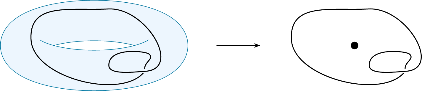
To contrast with the classical case, we will often call such a projection a dotted diagram. An example of a knot sitting in a solid torus and a corresponding dotted diagram appear in Figure 1. We generally conflate the notion of a ‘link in a solid torus’ with its ‘link diagram in the punctured disk’ and simply speak of a link diagram in the solid torus.

To define a Jones-type polynomial invariant in this setting, we work within the Kauffman bracket skein module of a link diagram D in the solid torus developed by Bataineh and Hajij in [Reference Bataineh and Hajij1]. The bracket $\langle \cdot \rangle $ in the variables A and t is defined by

Let $ R = \mathbb {Z}[A^{\pm 1}, t] $ . The Kauffman bracket skein module $ \mathcal {S}(M) $ is the $ R $ -module generated by isotopy classes of framed unoriented links in $ M $ , modulo the Kauffman bracket relations shown above.

The module $ \mathcal {S}(M) $ has a natural basis indexed by the number of parallel copies of the core curve of the torus. That is, any link can be resolved via the skein relations into a linear combination of powers of a generator $ t $ , where $ t $ denotes a longitude of the torus.

The skein module of the solid torus is the free $\mathbb {Z}[A^{\pm 1}]$ -module generated by powers of t and the above sum gives a well-defined skein element. For an oriented diagram D with writhe $w(D)$ , we normalise as in the case of $S^{3}$ to obtain the Jones polynomial.

The Jones polynomial $ V_L(q, t) $ for a framed link $ L \subset S^1 \times D^2 $ is derived from the normalised Kauffman bracket as follows.

• • Let $ \langle D \rangle \in \mathcal {S}(S^1 \times D^2) $ be the Kauffman bracket of a diagram D of a link $ L $ , expressed in the basis $ \{1, t, t^2, \ldots \} $ .

• • Each basis element $ t^n $ corresponds to $ n $ parallel longitudes (a cable of the core).

• • Apply the writhe correction and change variables to obtain a Jones polynomial for links in the thickened surface, invariant among all diagrams of the link L,

  $$ \begin{align*} V_L(q, t) = (-A^3)^{-w(D)} \langle D \rangle |_{A = q^{-1/4}}, \end{align*} $$
  where $ w(D) $ is the writhe of the diagram (the number of positive crossings minus the number of negative crossings ).

When we only consider one link L, we will generally write simply V instead of $V_L$ .

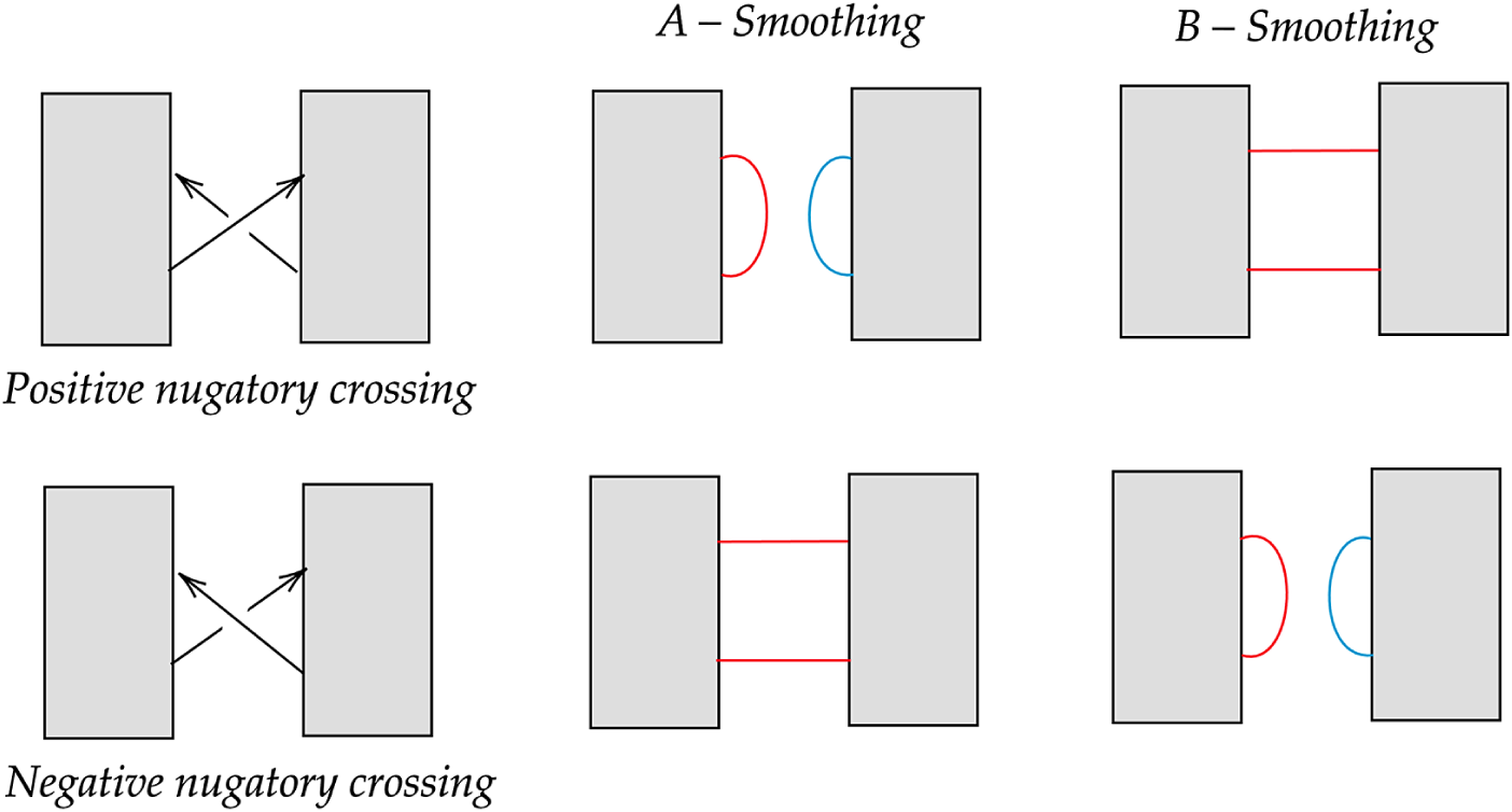
Equivalently, let S be a Kauffman state of D, that is, a choice of A- or B-smoothing at each crossing. Write $a(S)$ and $b(S)$ for the number of A- and B-smoothings, respectively (see Figure 2).

Figure 1

A link in a solid torus (left) and its dotted diagram (right).

Then, we express $\langle D \rangle $ as a sum over the contributions from each state $S_\sigma $ as

(2.1) $$ \begin{align} \langle D\rangle \;=\; \sum_{\sigma} A^{\,a(S_\sigma)-b(S_\sigma)}\, (-A^{2}-A^{-2})^{|S_\sigma|-1}t^{|T_\sigma|}, \end{align} $$

where $|S_\sigma |$ is the total number of circles in the state, $|T_\sigma |$ is the number of circles that ‘go around the dot’, $a(S_\sigma )$ is the number of A-smoothings in the state and $b(S_\sigma )$ is the number of B-smoothings in the state.

Figure 2

A crossing (left), its A-smoothing (middle) and its B-smoothing (right).

The Jones polynomial in a solid torus is sensitive to winding: links that are isotopic in $ S^3 $ , but differ in their winding around the core of $ S^1 \times D^2 $ , generally have different Jones polynomials. If a link lies in a 3-ball embedded in a solid torus, its Jones polynomial agrees with the classical Jones polynomial in $ S^3 $ .

We can also look at this as $\langle D \rangle = \sum _\sigma \langle D | S_\sigma \rangle $ , where the contribution of a single state $S_\sigma $ to $\langle D \rangle $ is

(2.2) $$ \begin{align} \mathit{contribution\ of\ state}\ S_\sigma = \langle D | S_\sigma \rangle = A^{a(S_\sigma)-b(S_\sigma)}(-A^{2}-A^{-2})^{|S_\sigma|-1}t^{|T_\sigma|}. \end{align} $$

As with the classical Kauffman bracket, we have the following result for the bracket polynomial for links in a solid torus.

Proposition 2.2. For any link diagram D in a solid torus,

$$ \begin{align*}\max\deg_A \langle D\rangle \leq \max\deg_A (\text{contribution of the all-}A\, \text{state})= \max \deg_A \langle D | S_A \rangle \end{align*} $$

and

$$ \begin{align*}\min\deg_A \langle D\rangle \geq \min\deg_A (\text{contribution of the all-}B\, \text{state}) = \min\deg_A \langle D | S_B \rangle. \end{align*} $$

Proposition 2.3. For any link diagram D in a solid torus with n crossings,

$$ \begin{align*}\operatorname{\mathrm{span}} \langle D \rangle \leq 4n.\end{align*} $$

Proof. From Proposition 2.2,

$$ \begin{align*} \operatorname{\mathrm{span}} V_D &= \max \deg_A \langle D \rangle - \min\deg_A \langle D \rangle \\ & \leq \max\deg_A \langle D | S_A \rangle - \min\deg_A \langle D | S_B \rangle \\ & = a(S_A) - b(S_A) + 2(|S_A|-1) - ( a(S_B) - b(S_B) - 2(|S_B|-1))\\ & = n + 2(|S_A| -1) - (-n - 2(|S_B| - 1) )\\ & = 2n + 2(|S_A| + |S_B|-2)\\ & \leq 2n + 2n = 4n.\\[-37pt] \end{align*} $$

3 Dotted-reduced diagrams

We now introduce the notions of reduced and dotted-reduced diagrams for knots in a solid torus.

3.1 Reduced and dotted-reduced diagrams

In classical knot theory, a crossing c in a knot diagram is nugatory if we can draw a simple closed curve in the projection disk such that the curve intersects the diagram only at the double point of the crossing c. We analogously define nugatory crossings appearing in diagrams of links in a solid torus, described at the start of Section 2.

Definition 3.1. In a diagram of a link in a solid torus, a crossing c is called nugatory if we can draw a simple closed curve in the projection punctured disk such that the curve intersects the diagram only at the double point of the crossing c.

In classical knot theory, a diagram is called reduced if it does not have any nugatory crossings. The idea is that any nugatory crossing can be ‘removed’ by twisting one half of the diagram. In the setting of a solid torus, not all nugatory crossings can actually be undone that way, as the structure of the solid torus may prevent such twists.

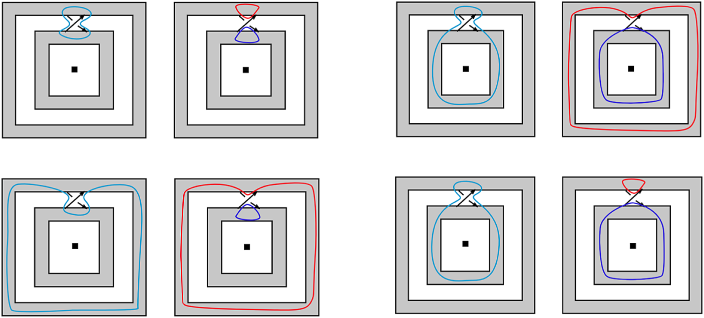
Definition 3.2. Let D be a link diagram in a solid torus, represented as a dotted diagram, with a crossing c that is nugatory as in Definition 3.1. If we can draw a simple closed curve in the projection punctured disk that intersects D only in the double point of the crossing c such that the curve is contractible in the projection punctured disk, then we say the crossing is dotted-reducible (see Figure 3). If instead all such curves are not contractible, then we say the crossing is dotted-irreducible.

What we call dotted-irreducible crossings for diagrams in a solid torus are comparable to Boden, Karimi and Sikora’s essential crossings for diagrams in a thickened surface in [Reference Boden, Karimi and Sikora3].

Definition 3.3. A link diagram in a solid torus is dotted-reduced if it has no nugatory crossings or if its only nugatory crossings are dotted-irreducible crossings.

We can now state our main result, which is proved in the next section.

Theorem 3.4. Let D be an alternating dotted-reduced link diagram in a solid torus with n crossings. Then, $\operatorname {\mathrm {span}} \langle D \rangle = 4n$ .

We then relate this Kauffman bracket polynomial for links in a solid torus to the corresponding Jones polynomial for links in a solid torus, giving two corollaries.

Corollary 3.5. Let D be an alternating dotted-reduced link diagram in a solid torus with n crossings. Then, $\operatorname {\mathrm {span}} V = n(D)$ .

Proof. This follows from the construction of V from $\langle D \rangle $ and Theorem 3.4.

Corollary 3.6. An alternating dotted-reduced diagram of a link in a solid torus is minimal with respect to crossing number.

Figure 3

Removing dotted-reducible crossings.

Figure 3 Long description

There are eight panels in two rows and four columns. Each panel contains four nested squares with a central black square. In the top-left panel, a small blue loop crosses itself at the topmost edge of the innermost square. The next panel to the right shows a red loop above a blue loop, both crossing at the top. The third panel shows a larger blue loop crossing itself at the top edge of the second square. The fourth panel shows a large red loop outside all squares and a blue loop inside, both crossing at the top. The bottom row repeats this pattern with the loops progressively expanding outward and the crossings becoming fewer. The final panel at bottom-right shows a large red loop outside all squares and a blue loop inside, both without crossings.

Proof. The proof is analogous to the proof for the classical case. For an alternating dotted-reduced diagram D, by Corollary 3.5, $\operatorname {\mathrm {span}} V \leq n(L) \leq n(D) = \operatorname {\mathrm {span}} V$ , so D must be a minimal diagram.

4 Proof of the main theorem

Now, we begin to prove Theorem 3.4. In the proof of Proposition 2.3, we obtain

$$ \begin{align*}\operatorname{\mathrm{span}} \langle D \rangle \leq \max\deg_A\langle D |S_A \rangle - \min\deg_A \langle D |S_B \rangle = 2n + 2(|S_A| + |S_B| -2) \leq 4n.\end{align*} $$

From classical knot theory, if D is an alternating diagram, then $|S_A|+|S_B| = n + 2$ and so the last inequality is an equality [Reference Kauffman4]. This holds regardless of whether or not the diagram is reduced (in a classical sense), so it still holds in the dotted-reduced setting.

To show that in an alternating dotted-reduced diagram we have $\operatorname {\mathrm {span}} \langle D \rangle = 4n$ , it remains to show that the first inequality must also be an equality.

Theorem 4.1. Let D be an alternating dotted-reduced link diagram in a solid torus. Then,

$$ \begin{align*}\max\deg_A \langle D\rangle = \max\deg_A (\text{contribution of the all-}A\, \text{state})= \max\deg_A \langle D |S_A \rangle\end{align*} $$

and

$$ \begin{align*}\min\deg_A \langle D\rangle = \min\deg_A (\text{contribution of the all-}B\, \text{state}) = \min\deg_A \langle D |S_B \rangle. \end{align*} $$

Proof. By symmetry, it suffices to prove the first statement. We claim that the contribution of the all-A state to the bracket polynomial is not cancelled out by the contribution of any other state.

Suppose for a contradiction that it does cancel out. Then, there is some other state $S_\sigma $ with $\max \deg _A\langle D | S_\sigma \rangle = \max \deg _A \langle D | S_A \rangle $ , and so

$$ \begin{align*} \underset{=\max\deg_A\langle D | S_\sigma \rangle}{\underbrace{a(S_\sigma)-b(S_\sigma) + 2(|S_\sigma| - 1)}} = \underset{=\max\deg_A \langle D | S_A \rangle}{\underbrace{n + 2(|S_A| - 1)}}. \end{align*} $$

Since $a(S_\sigma )-b(S_\sigma ) = n-2b(S_\sigma )$ , this is equivalent to $|S_\sigma | = |S_A| + b(S_\sigma )$ .

Consider $\widetilde {D}$ , the image of D under the obvious lift from $A \times I$ to $\mathbb R^2 \times I$ . Since we want to find the total number of A-circles, and the number of A-circles in D is the same as the number of A-circles in $\widetilde {D}$ , we can consider $\widetilde {D}$ and leverage what we know about classical diagrams. In a reduced alternating classical diagram $\widetilde {D}$ , any state adjacent to $S_A$ will have one fewer circle than $S_A$ . However, if the alternating diagram has nugatory crossings, there may be states adjacent to $S_A$ that have more circles.

Proof. Let $S_\sigma $ be a state satisfying $|S_\sigma | = |S_A| + b(S_\sigma )$ . Then, $S_\sigma $ is obtained from $S_A$ by changing the smoothings on a sequence of $b(S_\sigma )$ crossings such that at every step in the sequence, the total number of circles in the resulting state increases by one.

Starting with $S_A$ and changing the smoothing of a nonnugatory crossing will decrease the number of circles. So, $S_\sigma $ must be obtained by changing the smoothing at a nugatory crossing.

Figure 4

Smoothing crossings.

Figure 4 Long description

The diagram has two rows and three columns. The top row is labeled Positive nugatory crossing, the bottom row Negative nugatory crossing. In each row, the left panel shows two rectangles with arrows indicating the crossing direction. The middle panel, labeled A–Smoothing, shows the left rectangle with a red arc and the right with a blue arc, forming two loops. The right panel, labeled B–Smoothing, shows two horizontal red lines connecting the rectangles. In the bottom row, the left panel shows arrows indicating the opposite crossing direction. The middle panel shows two horizontal red lines connecting the rectangles. The right panel shows a red arc on the left and a blue arc on the right, forming two loops.

In Figure 4, we see that a state $S_\sigma $ adjacent to $S_A$ will have $|S_\sigma | = |S_A| + 1$ if and only if $S_\sigma $ is obtained from $S_A$ by performing a B-smoothing on a negative nugatory crossing. Similarly, any state $S_\sigma $ will have $|S_\sigma | = |S_A| + b(S_\sigma )$ if and only if $S_\sigma $ is obtained from $S_A$ by performing B-smoothings on $b(S_\sigma )$ negative nugatory crossings.

Proof. Consider two states $S_\sigma '$ and $S_\sigma $ that differ only at some negative dotted-irreducible crossing x. If $S_\sigma '$ is the state with $x\ A$ -smoothed and $S_\sigma $ is the state with $x\ B$ -smoothed, then either $|T_\sigma | = |T_\sigma '|$ or $|T_\sigma | = |T_\sigma '| + 2$ . This is shown in Figure 2. So, if $S_\sigma $ is obtained from $S_A$ by successively changing the smoothing at negative dotted-irreducible crossings (changing from A-smoothings to B-smoothings), then $|T_\sigma | \geq |T_A|$ .

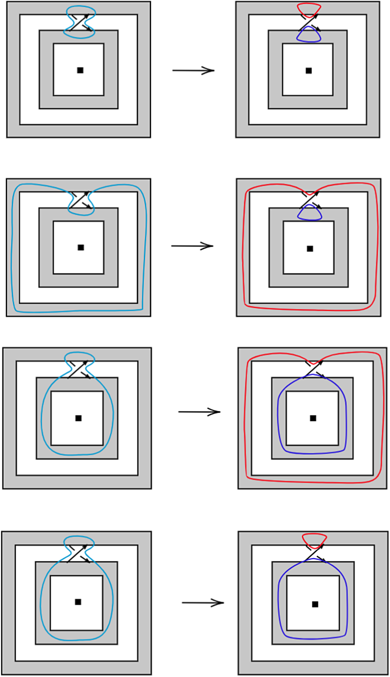
Now, consider what happens when we start with the all-A state and change the smoothing at just one negative dotted-irreducible crossing. Call this state $S_\sigma '$ . Since the diagram is dotted-reduced and alternating, the A-state must look like the example shown in Figure 5: the circle in the A-state that meets itself at this negative dotted-irreducible crossing does not go around the dot. When we change the smoothing at this crossing to be a B-smoothing, we obtain two circles that go around the dot, as in the last row of Figure 5. Then, the number of circles that go around the dot in $S_\sigma '$ is $|T_\sigma '| = |T_A| + 2$ .

Figure 5

In each of the four rows, we have on the left a state S in which our negative dotted-irreducible crossing is given an A-smoothing, and on the right the adjacent state $S'$ which is identical to S except at that one crossing. The four rows show each of the four possibilities for how a state circle involving this crossing could interact with the rest of the diagram.

Figure 5 Long description

There are four rows, each with two panels. In each row, the left panel shows a square grid with a black square at the center and a blue state circle interacting with a negative crossing at the top. The right panel shows the same grid, but the state circle is now split into two colored loops, red and purple, after an A-smoothing at the crossing. Row one: the blue loop is small and local to the crossing; after smoothing, it splits into a small red loop and a small purple loop. Row two: the blue loop is large, encircling the outermost square; after smoothing, the red loop is large and the purple loop is small. Row three: the blue loop is large, encircling the central square; after smoothing, the red loop is large and the purple loop is medium-sized. Row four: the blue loop is medium-sized, encircling the central square; after smoothing, the red loop is small and the purple loop is medium-sized. Each arrow between panels indicates the transformation from the left state to the right state.

So, if $S_\sigma $ is obtained from $S_A$ by changing some number of negative dotted-irreducible crossings, then $|T_\sigma | \geq |T_\sigma '| = |T_A| + 2> |T_A|$ .

Thus, any state $S_\sigma $ which has the same $\max \deg _A$ as $S_A$ will not have the same value of $|T|$ , so the contributions of $S_\sigma $ and $S_A$ cannot cancel out in the Kauffman bracket for links in the solid torus. Therefore, the contribution of the all-A state to the Jones polynomial does not cancel out and we have $\max \deg _A \langle D \rangle = \max \deg _A \langle D | S_A \rangle $ .

This completes the proof of Theorem 4.1.