3.1. Problem settings

In this section the asymptotic analysis is carried out for the nonlinear penalized vorticity equation (2.3) with respect to time. As the target situation, the initial flow around an impulsively started circular cylinder is selected. The previous theoretical study of this target flow can be found in Bar-Lev & Yang (Reference Bar-Lev and Yang1975). They introduced a small parameter $\epsilon = U_o T_o / l_o$ where $l_o$, $T_o$ and $U_o$ are the reference length, time and velocity, respectively. In their analysis the length $l_o$ is taken as the radius of a cylinder, $U_o$ is the constant moving velocity and $T_o$ is the time. Moreover, the dimensionless time is defined as $t = ( U_o / l_o ) t^*$ with respect to $l_o$ and $U_o$. Here, $t^*$ denotes the actual dimensional time.

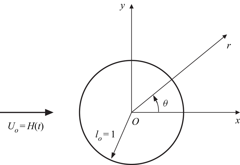
Figure 1 illustrates the problem setting on the relative coordinate system fixed with the centre of the cylinder. In figure 1 the orthogonal coordinate system $( x, y )$ and the polar coordinate system $( r, \theta )$ are taken, and the origin O is set at the centre of the circular cylinder. This study considers the flow past an impulsively started translating circular cylinder at $t = 0$ in a quiescent fluid. In the relative coordinate system, this flow is replaced by the situation that the circular cylinder is abruptly immersed in the uniform flow at $t = 0$, i.e. $U = U_o H ( t )$ where $H ( t ) = 0$ for $t \leqslant 0$ and $H ( t ) = 1$ for $t > 0$. Therefore, the vorticity can be found to be zero ($\omega = 0$) at $t = 0$.

Figure 1.

Notations for a circular cylinder abruptly immersed in a constant uniform stream.

The target issue is then reduced to a singular perturbation problem with respect to $\epsilon$ for the penalized vorticity equation (2.3). We introduce a stretched time $T$ which is defined as $t = \epsilon T$, along the lines of the analysis by Bar-Lev & Yang (Reference Bar-Lev and Yang1975). Because the penalization parameter $\lambda$ is taken to be proportional to the inverse of the time step size $\delta t$ (i.e. $\lambda = \alpha / \delta t$ with the relaxation coefficient $\alpha$ in Hejlesen et al. (Reference Hejlesen, Koumoutsakos, Leonard and Walther2015)), we set $\lambda$ as $\lambda = \lambda _o / \epsilon$ with $\lambda _o = O( 1 )$. To compare with the analytical results of Bar-Lev & Yang (Reference Bar-Lev and Yang1975), we assume that the Reynolds number $\mbox {{Re}}$ is sufficiently large, that is, the kinematic viscosity $\nu$ is sufficiently small. Therefore, we can set $\nu = \epsilon \nu _o$ with $\nu _o = O( 1 )$. The penalized governing equation (2.3) is then written as

(3.1)\begin{equation} \frac{\partial {\omega}}{\partial T} + \epsilon {\boldsymbol u} \boldsymbol{\cdot} {\boldsymbol \nabla} {\omega} = \epsilon^2 \nu_o \nabla^2 {\omega} - \lambda_o {\boldsymbol \nabla} \times \left( \chi {\boldsymbol u} \right). \end{equation}

Note that (3.1) is the dimensionless form with respect to $U_o$ and $l_o$ so that $\nu _o$ can be found to be the dimensionless kinematic viscosity. Moreover, this study takes the relative coordinate system fixed with the cylinder, and therefore the velocity of the solid body is ${\boldsymbol u}_S = 0$.

3.2. Outer solutions

We first consider the outer solution $\omega _F^o$ (denoted by the superscript $o$) of the governing equation (3.1) in the fluid domain. To do so, $\omega _F^o$ is asymptotically expressed as, using the small parameter $\varDelta$ that is a function of $\epsilon$,

(3.2)\begin{equation} \omega^o_F = \omega^o_{F0} + \sum_{n = 1}^\infty \varDelta^n \omega^o_{Fn}. \end{equation}

The outer solution of the fluid velocity ${\boldsymbol u}^o_F$ is also expressed as

(3.3)\begin{equation} {\boldsymbol u}^o_F = {\boldsymbol u}^o_{F0} + \sum_{n = 1}^\infty \varDelta^n {\boldsymbol u}^o_{Fn}. \end{equation}

Since in the fluid domain ${\mathscr F}$ the characteristic function is $\chi = 0$, (3.1) reduces to $\partial \omega _{F0}^o / \partial T = 0$. Therefore, we can easily find $\omega _{F0}^o = 0$. Similarly, carrying out the recursive calculation in (3.1), we have $\omega _F^o$ at the order $n$ as

(3.4)\begin{equation} \omega^o_{F n} = 0, \quad \text{for}\ n = 0, 1, 2, \ldots. \end{equation}

Inside the body ${\mathscr S}$ the flow is described by (3.1) set at $\chi = 1$. Since the cylinder is quiescent at $t \le 0$, the initial vorticity inside the body $\omega _{S}^o$ is zero.

The circular cylinder impulsively immersed in a constant uniform flow at $t = 0$. Noting that $\omega ^o_{F0} = 0$ in (3.4), at the early stage of motion, the dominant order of the outer solution in the fluid domain is described by the potential flow solution, i.e.

(3.5)\begin{equation} \psi_0^o = \left( r - \frac{1}{r} \right) H( T ) \sin{\theta}, \quad \text{for} \ r > 1, \end{equation}

where $\psi$ indicates the stream function whose asymptotic expansion is defined as $\psi = \psi _0^o + \sum _{n = 1}^\infty \varDelta ^n \psi _n^0$. Here, the polar coordinates are taken as $( r, \theta )$ and they are mainly taken in the following sections. Indeed, at the early stage of motion, the higher-order solutions as well as the dominant-order solution of the outer fluid flow are governed by the potential flow (see Bar-Lev & Yang Reference Bar-Lev and Yang1975). We can therefore express the stream function at the order $n$ as

(3.6)\begin{equation} \psi^o_n = \sum_{m = 1} \frac{1}{r^m} \left[ A_{mn}^o ( T ) \sin{m \theta} + B_{mn}^o ( T ) \cos{m \theta} \right], \quad \text{for}\ r > 1. \end{equation}

where $A_{mn}^o$ and $B_{mn}^o$ are indeterminate functions of $T$, respectively. These indeterminate functions can be determined by the matching with the inner solutions (see the following subsection).

3.3. Inner solutions

The outer flow of (3.5) causes the slip velocity on the surface of the cylinder (at $r = 1$) so that a non-uniformity domain can be found to exist near the cylinder surface. To remedy this, we stretch the radial coordinate $r$ to $R$ that is defined by $R = ( r - 1 ) / \epsilon$. Then, (3.1) is written as

(3.7) $$\begin{gather} \frac{\partial \omega}{\partial T} + u_r \frac{\partial \omega}{\partial R} + \frac{\epsilon}{1 + \epsilon R} u_\theta \frac{\partial \omega}{\partial \theta} = \nu_o \left( \frac{\partial^2}{\partial R^2} + \frac{\epsilon}{1 + \epsilon R} \frac{\partial}{\partial R} + \frac{\epsilon^2}{( 1 + \epsilon R )^2} \frac{\partial^2}{\partial \theta^2} \right) \omega \nonumber\\ - \frac{\lambda_o}{\epsilon} \frac{\partial ( \chi u_\theta )}{\partial R} + \frac{\lambda_o \chi}{1 + \epsilon R} \frac{\partial u_r}{\partial \theta} - \frac{\lambda_o \chi}{1 + \epsilon R} u_\theta, \end{gather}$$

where $u_r$ and $u_\theta$ are the velocity components of the radial ($r$) and tangential ($\theta$) directions, respectively. Also, the continuity equation and the vorticity are, respectively, written as

(3.8a,b)\begin{equation} \frac{\partial u_r}{\partial R} + \frac{\epsilon}{1 + \epsilon R} \left( u_r + \frac{\partial u_\theta}{\partial \theta} \right) = 0, \quad \omega = \frac{1}{\epsilon} \left[ \frac{\partial u_\theta}{\partial R} + \frac{\epsilon}{1 + \epsilon R} \left( u_\theta - \frac{\partial u_r}{\partial \theta} \right) \right]. \end{equation}

Taking into account (3.8a,b), the velocity components of $u_r$ and $u_\theta$ and the vorticity $\omega$ are asymptotically expressed as, in the inner domain (denoted by the superscript $i$),

(3.9a–c)\begin{equation} u_r^i = u_{r0}^i + \sum_{n = 1} \epsilon^n u_{rn}^i, \quad u_\theta^i = u_{\theta 0}^i + \sum_{n = 1} \epsilon^n u^i_{\theta n}, \quad \omega^i = \frac{1}{\epsilon} \left( \omega_0^i + \sum_{n = 1} \epsilon^n \omega_n^i \right). \end{equation}

3.4. First-order approximation

Here, the first equation of (3.8a,b) is found to reduce to $\partial u_{r0}^i / \partial R = 0$ for $u_{r0}^i$. The inner expansion of the first-order outer solution $u_{rF}^o$ needs to be $u_{rF}^{oi} = 2 \epsilon R H ( T ) \cos {\theta }$ because of (3.5). The matching between $u_{Fr}^{oi}$ and $u_{r0}^{io}$ (i.e. $u_{Fr}^{oi} = u_{r0}^{io}$) then yields

(3.10)\begin{equation} u_{r0}^i = 0. \end{equation}

Note that (3.10) satisfies the matching of the solution inside the body (because of ${\boldsymbol u}_S = 0$). Substituting (3.9a–c) into (3.7) and using (3.10) and the relation of 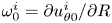$\omega _0^i = \partial u_{\theta 0}^i / \partial R$ which is obtained from the second equation of (3.8a,b), we can obtain the first-order solution of $\omega ^i$ as, from (3.7),

(3.11)\begin{equation} \frac{\partial \omega_0^i}{\partial T} = \nu_o \frac{\partial^2 \omega_0^i}{\partial R^2} - \lambda_o \omega_0^i - \lambda_o \frac{{\textrm{d}} \chi}{{\textrm{d}} R} u_{\theta0}^i. \end{equation}

On the boundary of the cylinder surface, the vorticity is assumed to be continuous as

(3.12)\begin{equation} \lim_{R \to 0+} \omega_0^i = \lim_{R \to 0-} \omega_0^i, \end{equation}

where $R \to 0+$ and $R \to 0-$ means $R \to 0$ from $R > 0$ and from $R < 0$, respectively. From the above relation, we have for $R > 0$ and $R < 0$ that

(3.13)\begin{equation} \frac{\partial \omega_0^i}{\partial T} = \nu_o \frac{\partial^2 \omega_0^i}{\partial R^2} - \left\{ \begin{array}{@{}ll} 0 & \text{for}\ R > 0, \\ \lambda_o\omega_0^i & \text{for}\ R < 0. \end{array} \right. \end{equation}

The Laplace transform facilitates the analysis of (3.13) because the circular cylinder impulsively starts from rest at $t = 0$. The Laplace transform of $\omega _0^i$ is defined as $\varOmega _0^i = {\mathscr L} [ \omega _0^i ] = \int _0^\infty e^{- s T} \omega _0^i ( R, \theta ; T ) \,{\textrm {d}} T$ where $s$ is the Laplace complex variable. Then, (3.13) is written as

(3.14)\begin{equation} \frac{\partial^2 \varOmega_0^i}{\partial R^2} = \frac{1}{\nu_o} \times \left\{ \begin{array}{@{}ll} s \varOmega_0^i & \text{for}\ R > 0,\\ ( s + \lambda_o ) \varOmega_0^i & \text{for} \ R < 0. \end{array} \right. \end{equation}

As mentioned above, the outer solutions are described by a potential flow inside the fluid domain and ${\boldsymbol u}_S = 0$ inside the cylinder. Taking into account the matching with the outer solutions, we can easily find $\varOmega _0^i \to 0$ for $R \to \pm \infty$. Furthermore, the vorticity $\omega _0^i$ is continuous at $R = 0$. Therefore, the solution to (3.14) is obtained as

(3.15)\begin{equation} \varOmega_0^i = \left\{ \begin{array}{@{}ll} A_0 e^{- \sqrt{s / \nu_o} R} & \text{for}\ R > 0, \\ A_0 e^{\sqrt{( s + \lambda_o ) / \nu_o} R} & \text{for}\ R < 0, \end{array} \right. \end{equation}

where $A_0$ is an indeterminate function of $s$ and $\theta$. We note that $\partial \omega _{0}^i / \partial R$ is discontinuous at $R = 0$, i.e. in the present problem there is the slip induced by the radial gradient of the vorticity on the cylinder surface.

Similar to $\omega _0^i$, the Laplace transform of $u_{\theta 0}^i$ is described by $U_{\theta 0}^i = {\mathscr L} [ u_{\theta 0}^i ]$. Substituting (3.15) into the relation of $\omega _0^i = \partial u_{\theta 0}^i / \partial R$ which is obtained from the second equation of (3.8a,b), we can obtain

(3.16)\begin{equation} U_{\theta 0}^i = \left\{ \begin{array}{@{}ll} \displaystyle -A_0 \sqrt{\dfrac{\nu_o}{s}} e^{- \sqrt{s / \nu_o} R} + A_1 & \text{for}\ R > 0, \\ \displaystyle A_0 \sqrt{\dfrac{\nu_o}{s + \lambda_o}} e^{\sqrt{( s + \lambda_o ) / \nu} R} + A_1 - \left( \sqrt{\dfrac{\nu_o}{s}} + \sqrt{\dfrac{\nu_o}{s + \lambda_o}} \right) A_0 & \text{for}\ R < 0, \end{array} \right. \end{equation}

where $A_1$ is an indeterminate function of $s$ and $\theta$. We notice that in the derivation of (3.16) we employed the continuity of $U_{\theta 0}^i$ at $R = 0$, i.e.

(3.17)\begin{equation} \lim_{R \to 0+} u_{\theta 0}^i = \lim_{R \to 0-} u_{\theta 0}^i. \end{equation}

The matching between the outer expansion of (3.16) (i.e. $U_{\theta 0}^{io}$) and the inner expansion of (3.5) (i.e. ${\mathscr L} [ u_{\theta 0}^{oi} ]$) can determine the indeterminate function $A_1$ as $A_1 = - ( 2 / s ) \sin {\theta }$. As for the solid domain, the matching with the inner expansion of $u_S^o$ (i.e. $u_S^{oi} = 0$) determines the indeterminate function $A_1$ as $A_1 = A_0 \{ ( \nu _o / s)^{1/2} + [ \nu _o / ( s + \lambda _o ) ]^{1/2} ]\}$. Therefore, the first approximation of the inner solution for the velocity, $u_{\theta 0}^i$, can be written as

(3.18)\begin{equation} u_{\theta 0}^i = \sin{\theta} \times \left\{ \begin{array}{@{}ll} u_{\theta 0}^+ & \text{for}\ R > 0, \\ u_{\theta 0}^- & \text{for} \ R < 0, \end{array} \right. \end{equation}

where

(3.19)$$\begin{gather} u_{\theta 0}^+{=} {\mathscr L}^{{-}1} \left[ - \frac{2}{s} + \frac{2}{\lambda_o} \frac{\sqrt{s + \lambda_o}}{s} \left( \sqrt{s + \lambda_o} - \sqrt{s} \right) e^{ - \sqrt{s / \nu_o} R} \right], \end{gather}$$

(3.20)$$\begin{gather}u_{\theta 0}^-{=} - {\mathscr L}^{{-}1} \left[ \frac{2}{\lambda_o} \frac{\sqrt{s + \lambda_o} - \sqrt{s}}{\sqrt{s}} e^{\sqrt{( s + \lambda_o ) / \nu_o } R} \right]. \end{gather}$$

The inverse Laplace transform of (3.19) and (3.20) are calculated by using the formulae ${\mathscr L}^{-1} [ \sqrt {{\rm \pi} / s} \, e^{- a \sqrt {s}} ] = e^{- a^2 / ( 4 t )} / \sqrt {t}$ for $a \geqslant 0$, ${\mathscr L}^{-1} [ ( 2 \sqrt {{\rm \pi} } \, e^{- a \sqrt {s}} ) / a ] = e^{- a^2 / ( 4 t )} / t^{3 / 2}$ for $a > 0$, and ${\mathscr L}^{-1} [ \sqrt {( s + 2 a ) / s} - 1 ] = a e^{- a t} ( I_1 ( a t ) + I_0 ( a t ) )$ where $I_n$ ($n = 0$, $1$) is the modified Bessel function of the first kind (see Abramowitz & Stegun (Reference Abramowitz and Stegun1954), formulae 29.3.84, 29.3.82 and 29.3.48). For $R > 0$, (3.18) becomes, taking the inverse Laplace transform of (3.19) and setting $\eta = R / ( 2 \sqrt {\nu _o T} )$,

(3.21) $$\begin{gather} u_{\theta 0}^i = \left\{ - 2 + 2 \, \text{erfc} ( \eta ) - \frac{\eta}{\sqrt{\rm \pi}} e^{- \lambda_o T / 2} \int_0^1 \frac{1}{x^{3 / 2}} e^{- \eta^2 / x + ( \lambda_o T / 2 ) x} \right.\nonumber\\ \left. \times \left[ I_1 \left( \frac{\lambda_o T}{2} ( 1 - x ) \right) + I_0 \left( \frac{\lambda_o T}{2} ( 1 - x ) \right) \right] \,{\textrm{d}} x \vphantom{\int_0^1}\right\} \sin{\theta}. \end{gather}$$

Similarly, for $R < 0$, (3.18) becomes

(3.22)$$\begin{gather} u_{\theta 0}^i = \frac{\eta}{\sqrt{\rm \pi}} e^{- \lambda_o T / 2} \int_0^1 \frac{1}{x^{3 / 2}} e^{- \eta^2 / x - ( \lambda_o T / 2 ) x} \nonumber\\ \times \left[ I_1 \left( \frac{\lambda_o T}{2} ( 1 - x ) \right) + I_0 \left( \frac{\lambda_o T}{2} ( 1 - x ) \right) \right] \,{\textrm{d}} x \sin{\theta}. \end{gather}$$

The slip velocity on the surface of the cylinder is calculated by setting $R = 0$ in (3.18) giving

(3.23)\begin{align} u_{\theta 0}^i ={-} \frac{2}{\lambda_o}{\mathscr L}^{{-}1} \left( \sqrt{\frac{s + \lambda_o}{s}} - 1 \right) \sin{\theta} ={-} e^{- \lambda_o T / 2} \left[ I_1 \left( \frac{\lambda_o T}{2} \right) + I_0 \left( \frac{\lambda_o T}{2} \right) \right] \sin{\theta}. \end{align}

It can be found that the tangential slip velocity at $R = 0$ decreases with $1 / \sqrt {\lambda _o}$, i.e. $u_{\theta 0}^i \to O( 1 / \sqrt {\lambda _o} )$ as $\lambda _o \to \infty$. We will later show that the normal slip velocity at $R=0$ is of the order of $1/\lambda _o$ as $\lambda _o\to \infty$, i.e. $u_{r1}^i \to O(1/\lambda _o)$. This result is the same as the one of Carbou & Fabrie (Reference Carbou and Fabrie2003) although the estimation given by Angot et al. 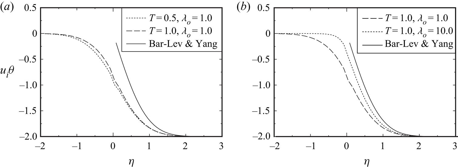(Reference Angot, Bruneau and Fabrie1999) is of the order of $1/\lambda _o^{1/4}$. Figure 2 shows the distribution of $u_{\theta 0}^i$ with respect to $\eta = R / ( 2 \sqrt {\nu _o T} )$ at $\theta = {\rm \pi}/ 2$ (along the $y$-axis). In the computation of figure 2, the twenty-points Gaussian integration is employed to estimate the integral. Figure 2 compares the first-order solution $u_{\theta 0}^i$ with respect to $T$ at fixed $\lambda _o = 1.0$ (figure 2a) and $\lambda _o$ at fixed $T = 1.0$ (figure 2b) against the analytical solution of Bar-Lev & Yang (Reference Bar-Lev and Yang1975) using the conventional Navier–Stokes equations. As shown in figure 2, the slip velocity arises on the surface of the cylinder, and the strength decreases with increasing $\lambda _o$. The strength of the slip velocity is of $O( 1 / \sqrt {\lambda _o T} )$. The velocity distribution of $u_{\theta 0}^i$ is observed to converge to the solution of Bar-Lev & Yang (Reference Bar-Lev and Yang1975) with increasing $\lambda _o$.

Figure 2.

Comparison of the first-order inner solutions of $u_\theta ^i$ at $\theta = {\rm \pi}/ 2$ against the result of Bar-Lev & Yang (Reference Bar-Lev and Yang1975).

Similar to (3.20), the first approximation of the inner solution for the vorticity, $\omega _0^i$, is written as

(3.24)\begin{equation} \omega_0^i = \sin{\theta} \times \left\{ \begin{array}{@{}ll} \tilde{\omega}_0^{i+} & \text{for}\ R > 0, \\ \tilde{\omega}_0^{i-} & \text{for}\ R < 0, \end{array} \right. \end{equation}

where

(3.25)$$\begin{gather} \tilde{\omega}_0^{i+} ={-}{\mathscr L}^{{-}1} \left[ \frac{2}{\lambda_o \sqrt{\nu_o}} \sqrt{\frac{s + \lambda_o}{s}} \left( \sqrt{s + \lambda_o} - \sqrt{s} \right) e^{- \sqrt{s / \nu_o} R} \right], \end{gather}$$

(3.26)$$\begin{gather}\tilde{\omega}_0^{i-} ={-}{\mathscr L}^{{-}1} \left[ \frac{2}{\lambda_o \sqrt{\nu_o}} \sqrt{\frac{s + \lambda_o}{s}} \left( \sqrt{s + \lambda_o} - \sqrt{s} \right) e^{\sqrt{( s + \lambda_o ) / \nu_o} R} \right]. \end{gather}$$

3.5. Second-order approximation

Moreover, we proceed to derive the second-order approximation. The first equation of (3.8a,b) gives the second-order inner solution $u_{r1}^i$ which is written by

(3.27)\begin{equation} \frac{\partial u_{r 1}^i}{\partial R} ={-} u_{r 0}^i - \frac{\partial u_{\theta 0}^i}{\partial \theta}. \end{equation}

Substituting (3.10) and (3.18) into (3.27) and taking into account the matching principle with ${\boldsymbol u}_S = 0$ that results in $u_{r1}^i \to 0$ as $R \to - \infty$, we have, using the continuity condition of $u_{r1}$ at $R = 0$,

(3.28)\begin{equation} u_{r1}^i = \cos{\theta} \times \left\{ \begin{array}{@{}ll} u_{r1}^+ & \text{for}\ R > 0, \\ u_{r1}^{-} & \text{for} \ R < 0, \end{array} \right. \end{equation}

where

(3.29)$$\begin{gather} u_{r1}^+{=} 2 {\mathscr L}^{{-}1} \left[ \frac{\sqrt{\nu_o}}{\lambda_o} \frac{\sqrt{s + \lambda_o} - \sqrt{s}}{s} \left( \sqrt{\frac{s + \lambda_o}{s}} e^{- \sqrt{s / \nu_o} R} - \frac{\lambda_o}{\sqrt{s ( s + \lambda_o )}} \right) +\frac{R}{s}\right], \end{gather}$$

(3.30)$$\begin{gather}u_{r1}^-{=} 2 {\mathscr L}^{{-}1} \left[ \frac{\sqrt{\nu_o}}{\lambda_o} \frac{\sqrt{s + \lambda_o} - \sqrt{s}}{\sqrt{s ( s + \lambda_o )}} e^{\sqrt{( s + \lambda_o ) / \nu_o} R} \right]. \end{gather}$$

From the above (3.18), $u_{r1}$ at $R=0$ becomes

(3.31)\begin{equation} u_{r1} = 2 \cos{\theta} \frac{1}{\lambda_o} \sqrt{\frac{\nu_o}{{\rm \pi} T}} \left( 1 - e^{- \lambda_o T} \right). \end{equation}

The normal slip velocity can be thus found to be of the order of $1 / \lambda _o$.

The outer solutions are obtained in (3.5) together with (3.6). The inner expansion of the outer solutions in the fluid domain is therefore written as, differentiating those equations with respect to $\theta$,

(3.32)\begin{equation} u_r^{oi} = 2 \epsilon R H ( T ) \cos{\theta} + \varDelta \sum_{n = 1} n \left( A_{n1}^o \cos{n \theta} - B_{n1}^o \sin{n \theta} \right). \end{equation}

The outer expansions of the inner solutions (3.18) and (3.28) are obtained for inside and outside the fluid domain. Equating these expansions for the fluid domain we can determine the indeterminate functions:

(3.33)\begin{equation} {\mathscr L} [ A_{n1}^o ] ={-} 2 \sqrt{\frac{\nu_o}{s ( s + \lambda_o )}} \frac{\sqrt{s + \lambda_o} - \sqrt{s}}{s} \delta_{n1}, \quad B_{n1}^o = 0, \quad \varDelta = \epsilon. \end{equation}

For the second-order vorticity $\omega _{1}^i$, (3.7) reads as

(3.34)$$\begin{gather} \frac{\partial \omega_{1}^i}{\partial T} + u_{r1}^i \frac{\partial \omega_0^i}{\partial R} + u_{r0}^i \frac{\partial \omega_{1}^i}{\partial R} + u_{\theta 0}^i \frac{\partial \omega_0^i}{\partial \theta} = \nu_o \frac{\partial^2 \omega_{1}^i}{\partial R^2} + \nu_o \frac{\partial \omega_0^i}{\partial R} \nonumber\\ - \lambda_o \frac{\partial}{\partial R} ( \chi u_{\theta 1}^i ) + \lambda_o \chi \frac{\partial u_{r 0}^i}{\partial \theta} - \lambda_o \chi u_{\theta 0}^i. \end{gather}$$

For the second-order vorticity the second equation of (3.8a,b) reduces to $\partial u_{\theta 1}^i / \partial R = \omega _1^i - u_{\theta 0}^i$. The Laplace transform of (3.34) gives, taking into account $u_{r0}^i = 0$,

(3.35) \begin{equation} \frac{{\textrm{d}}^2 \varOmega_1^i}{{\textrm{d}} R^2} - \left\{ \begin{array}{@{}ll} \displaystyle \dfrac{s}{\nu_o} \varOmega_1^i = F_+ ( R, \theta ) & \text{for} \ R > 0, \\ \displaystyle \dfrac{s + \lambda_o}{\nu_o} \varOmega_1^i = F_- ( R, \theta ) & \text{for} \ R < 0. \end{array} \right. \end{equation}

Here, the functions $F_{\pm } ( R, \theta )$ are defined for $R > 0$ and $R < 0$, respectively,

(3.36)\begin{equation} F_{{\pm}} ( R, \theta ) ={-} {\mathscr L} \left[ \frac{\partial \omega_0^i}{\partial R} - \frac{u_{r1}^i}{\nu _o} \frac{\partial \omega_0^i}{\partial R} - \frac{u_{\theta 0}^i}{\nu_o} \frac{\partial \omega_0^i}{\partial \theta} \right] = F_{{\pm}}^s \sin{\theta} + F_{{\pm}}^{cs} \sin{\theta} \cos{\theta}, \end{equation}

in which

(3.37a,b)\begin{equation} F_{{\pm}}^s ={-} {\mathscr L} \left[ \frac{\partial \tilde{\omega}_0^{i \pm}}{\partial R} \right], \quad F_{{\pm}}^{cs} ={-} {\mathscr L} \left[ \frac{u_{r1}^\pm}{\nu_o} \frac{\partial \tilde{\omega}_0^{i\pm}}{\partial R} + \frac{u_{\theta 0}^\pm}{\nu_o} \tilde{\omega}_0^{i \pm} \right]. \end{equation}

The ordinary differential equation of (3.36) can be easily solved as, taking into account the matching condition that $\varOmega _1^i \to 0$ as $R \to \pm \infty$,

(3.38)$$\begin{gather} \varOmega_1 ={-} \frac{e^{- a R}}{2 a} \int_0^R F_+ ( \xi, \theta ) e^{a \xi} \,{\textrm{d}} \xi - \frac{e^{a R}}{2 a} \int_R^\infty F_+ ( \xi, \theta ) e^{- a \xi} \,{\textrm{d}} \xi + D_0 e^{- a R} \quad \text{for}\ R > 0, \end{gather}$$

(3.39)$$\begin{gather}\varOmega_1 ={-} \frac{e^{- \hat{a} R}}{2 \hat{a}} \int_{- \infty}^R F_- ( \xi, \theta ) e^{\hat{a} \xi} \,{\textrm{d}} \xi - \frac{e^{\hat{a} R}}{2 \hat{a}} \int_R^0 F_- ( \xi, \theta ) e^{- \hat{a} \xi} \,{\textrm{d}} \xi + D_1 e^{\hat{a} R} \quad \text{for}\ R < 0, \end{gather}$$

where $a$ and $\hat {a}$ are, respectively, defined as

(3.40a,b)\begin{equation} a = \sqrt{\frac{s}{\nu_o}}, \quad \hat{a} = \sqrt{\frac{s + \lambda_o}{\nu_o}}. \end{equation}

In the derivation of (3.38) and (3.39), we used the fact that the integral constants $D_0$ and $D_1$ are functions of $s$ and $\theta$. Because the vorticity is continuous at $R = 0$, the constants $D_0$ and $D_1$ are linked with

(3.41)\begin{equation} D_0 - D_1 = \frac{1}{2 a} \int_0^\infty F_+ ( \xi, \theta ) e^{- a \xi} \,{\textrm{d}} \xi - \frac{1}{2 \hat{a}} \int_{- \infty}^0 F_- ( \xi, \theta ) e^{\hat{a} \xi} \,{\textrm{d}} \xi. \end{equation}

The second-order velocity $u_{\theta 1}^i$ is described by $\partial u_{\theta 1}^i / \partial R = \omega _1^i - u_{\theta 0}^i$ from the second equation of (3.8a,b) and (3.10). We here define the Laplace transform of $u_{\theta 1}^i$ as $U_{\theta 1}^i = {\mathscr L} [ u_{\theta 1}^i ]$. Furthermore, we note the matching condition that $U_{\theta 1}^i \to 0$ for $R \to - \infty$. For $R > 0$, we then have, using (3.19) and (3.38),

(3.42)$$\begin{gather} U_{\theta 1}^i = \frac{1}{2 a^2} \left( e^{- a R} \int_0^R F_+ ( \xi, \theta ) e^{a \xi} \,{\textrm{d}} \xi - e^{a R} \int_R^\infty F_+ ( \xi, \theta ) e^{- a \xi} \,{\textrm{d}} \xi \right) + \frac{1}{a^2} \int_R^\infty F_+ ( \xi, \theta) \,{\textrm{d}} \xi \nonumber\\ - \frac{D_0}{a} e^{- a R} + \left[ \frac{2}{s} R + \frac{2}{\lambda_o a} \frac{\sqrt{s + \lambda_o}}{s} \left( \sqrt{s + \lambda_o} - \sqrt{s} \right) e^{- a R} \right] \sin{\theta} + E_0. \end{gather}$$

For $R < 0$, we also have, using (3.20) and (3.39),

(3.43)$$\begin{gather} U_{\theta 1}^i = \frac{1}{2 \hat{a}^2} \left( e^{- \hat{a} R} \int_{-\infty}^R F_- e^{\hat{a} \xi} \,{\textrm{d}} \xi - e^{\hat{a} R} \int_R^0 F_- e^{- \hat{a} R} \,{\textrm{d}} \xi \right) - \frac{1}{\hat{a}^2} \int_{- \infty}^R F_- \,{\textrm{d}} \xi + \frac{D_1}{\hat{a}} e^{\hat{a} R} \nonumber\\ + \frac{2}{\lambda_a \hat{a}} \frac{\sqrt{s + \lambda_o} - \sqrt{s}}{\sqrt{s}} e^{\hat{a} R} \sin{\theta}. \end{gather}$$

The velocity $U_{\theta 1}^i$ is continuous at $R = 0$ and, therefore, we have

(3.44)$$\begin{gather} E_0 = \frac{D_0}{a} + \frac{D_1}{\hat{a}} + \frac{1}{a^2} \int_0^\infty F_+ \left( \frac{e^{- a \xi}}{2} - 1 \right) \,{\textrm{d}} \xi + \frac{1}{\hat{a}^2} \int_{- \infty}^0 F_- \left( \frac{e^{\hat{a} \xi}}{2} - 1 \right) \,{\textrm{d}} \xi \nonumber\\ + \left[ \frac{2}{\lambda_o \hat{a}} \frac{\sqrt{s + \lambda_o} - \sqrt{s}}{\sqrt{s}} - \frac{2}{\lambda_o a} \frac{\sqrt{s + \lambda_o}}{s} \left( \sqrt{s + \lambda_o} - \sqrt{s} \right) \right] \sin{\theta}. \end{gather}$$

The matching principle to the outer solution in the fluid domain can determine the function $E_0$ as, from (3.33),

(3.45)\begin{equation} E_0 = {\mathscr L} [ A_{11}^o ] \sin{\theta} ={-} 2 \sqrt{\frac{\nu_o}{s ( s + \lambda_o )}} \frac{\sqrt{s + \lambda_o} - \sqrt{s}}{s} \sin{\theta}. \end{equation}

We here consider the asymptotic behaviour of $u_{\theta 1}^i$ for $\lambda _o\gg 1$. Since $F_{\pm }$ is asymptotically expressed as, taking into account of the order of $u_{\theta 0}^i$ and $u_{r1}^i$, $F_{\pm }\sim F_{\pm }^0+({1}/{\sqrt {\lambda _o}})F_{\pm }^1+O(1/\lambda _o)$. Hence, we have $u_{\theta 1}^i \to O(1/\sqrt {\lambda _o})$. Furthermore, we easily have the following relations at $R = 0$ (i.e. on the cylinder surface), using the physical quantities:

(3.46)$$\begin{gather} u_{\theta 0}^i \sim{-} \frac{2 \sin{\theta}}{\sqrt{{\rm \pi} \lambda t}} \left[ 1 + O( 1 / ( \lambda t ) ) \right], \end{gather}$$

(3.47)$$\begin{gather}\frac{\partial u_{\theta 0}^i}{\partial r} \sim{-} \frac{2 \sin{\theta}}{\sqrt{{\rm \pi} \nu t}} \left[ 1 + O( 1 / ( \lambda t ) ) \right]. \end{gather}$$

Thus, we can have the following Navier condition on the tangential slip velocity from the first-order solution:

(3.48)\begin{equation} u_\theta - \sqrt{\frac{\nu}{\lambda}} \frac{\partial u_\theta}{\partial r} = 0. \end{equation}

The slip length $\alpha = \sqrt {\nu / \lambda }$ is of the order of $1 / \sqrt {\lambda }$ for $\lambda \gg 1$, and of the order of $\sqrt {1 / Re}$ for $Re \gg 1$, where $Re$ is the Reynolds number based on the radius of the cylinder and the impulsive constant velocity. This is in qualitatively agreement with the results given by Nguyen van yen et al. (Reference Nguyen van yen, Farge and Schneider2011, Reference Nguyen van yen, Kolomenskiy and Schneider2014).

3.6. Drag coefficient

In this subsection, we will derive the drag coefficient from the asymptotic solution which is obtained in the preceding subsections, and verify it against the results of Bar-Lev & Yang (Reference Bar-Lev and Yang1975). According to Bar-Lev & Yang (Reference Bar-Lev and Yang1975), the drag coefficient $C_D$ is defined as $C_D = D / [ ( 1 / 2 ) \rho U_o^2 ( 2 r_o ) ]$, where $U_o$ is a constant moving velocity and $r_o$ is the radius of a circular cylinder.

As formulated in (2.4), in the penalization method the drag force $D$ is obtained by the integration of the penalization term. Noting that (2.2) and ${\boldsymbol u}_s = 0$ (i.e. $|{\boldsymbol u}_s| \to 0$ as $R \to - \infty$), the drag force $D$ is written as

(3.49)\begin{align} D & = \rho \int_V \lambda \chi u_x \,{\textrm{d}} V = \rho \lambda_o \int_0^{2 {\rm \pi}} \int_{- 1 / \epsilon}^0 \left( u_r^i \cos{\theta} - u_{\theta}^i \sin{\theta} \right) ( 1 + \epsilon R ) \,{\textrm{d}} R \,{\textrm{d}} \theta \nonumber\\ & = \rho \lambda_o \int_0^{2 {\rm \pi}} \text{p.f.} \int_{- \infty}^0 \left( u_r^i \cos{\theta} - u_{\theta}^i \sin{\theta} \right) ( 1 + \epsilon R ) \,{\textrm{d}} R \,{\textrm{d}} \theta, \end{align}

in which the symbol ‘p.f.’ indicates the Hadamard finite part of integral and $u_x$ is the $x$ component of velocity. Noting that (3.9a–c) together with (3.10), (3.49) reduces to

(3.50)\begin{align} C_D & = \lambda_o \int_0^{2 {\rm \pi}} \int_{- \infty}^0 \left[ - u_{\theta 0}^{i} \sin{\theta} + \epsilon \left( u_{r1}^i \cos{\theta} - u_{\theta1}^i \sin{\theta} - R u_{\theta0}^i \sin{\theta} \right) \right] \,{\textrm{d}} R \,{\textrm{d}} \theta + O( \epsilon^2 ) \nonumber\\ & \approx \lambda_o {\rm \pi}\int_{- \infty}^0 \left[ - u_{\theta 0}^-{+} \epsilon \left( u_{r1}^-{-} u_{\theta 1}^{s-} - R u_{\theta 0}^- \right) \right] \,{\textrm{d}} R. \end{align}

Here, the function $u_{\theta 1}^{s-}$ indicates the components of $\sin {\theta }$ involved in $u_{\theta 1}^i$, i.e. $u_{\theta 1}^i = {\mathscr L}^{-1} [ U_{\theta 1}^i ] = u_{\theta 1}^{s-} \sin {\theta } + u_{\theta 1}^{cs-} \sin {\theta } \cos {\theta }$ for $R < 0$. Substituting the inverse Laplace transform of (3.20), (3.30) and (3.43) into (3.50), the drag coefficient $C_D$ is obtained as (see Appendix A for the detailed derivation)

(3.51)\begin{equation} C_D = 2 \sqrt{\frac{\nu_o {\rm \pi}}{T}} \left( 1 - e^{- \lambda_o T} \right) + {\rm \pi}\epsilon \nu_o \left[ 1 + e^{- \lambda_o T} - 2 e^{- \lambda_o T / 2} I_0 \left( \frac{\lambda_o T}{2} \right) \right]. \end{equation}

The above, (3.51), becomes as follows, when the physical quantities are replaced by $\lambda$, $t$ and $\nu$:

(3.52)\begin{equation} C_D = 2 \sqrt{\frac{\nu {\rm \pi}}{t}} \left( 1 - e^{- \lambda t} \right) + {\rm \pi}\nu \left[ 1 + e^{- \lambda t} - 2 e^{- \lambda t / 2} I_0 \left( \frac{\lambda t}{2} \right) \right]. \end{equation}

In the analytical result of Bar-Lev & Yang (Reference Bar-Lev and Yang1975) that is based on the conventional Navier–Stokes equations, the first-order solution of $C_D$ is obtained as $C_D = 4 \sqrt {\nu {\rm \pi}/ t}$. In contrast, the present result of (3.51) exhibits $C_D = 2\sqrt {\nu {\rm \pi}/ t}$ as $\lambda \to \infty$. It thus can be found that the first-order solution obtained from the penalization method is a half of the conventional result of Bar-Lev & Yang (Reference Bar-Lev and Yang1975) as $\lambda \to \infty$.

In the analysis of Bar-Lev & Yang (Reference Bar-Lev and Yang1975), the drag coefficient is derived from the sum of the friction drag and the pressure drag on the surface of the cylinder, i.e.

(3.53)\begin{equation} C_D = \epsilon \nu_o \int_0^{2 {\rm \pi}} \left( \frac{\partial \omega}{\partial r} - \omega \right)_{r = 1} \sin{\theta} \,{\textrm{d}} \theta. \end{equation}

The first term of the integral includes the contribution from the pressure and the second is the contribution from the friction. In their analysis the no-slip condition is imposed on the surface of the cylinder (i.e. $u_r^i = u_\theta ^i = 0$ at $R = 0$) and, therefore, we have $( 1 / \rho ) ( \partial p / \partial \theta ) = \nu _o ( \partial \omega ^i / \partial R )$ at $R = 0$. The penalization method does not enforce the no-slip condition on the surface of the cylinder so that such a relation could not fulfilled.

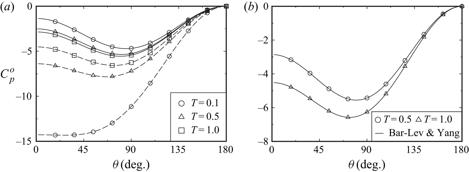
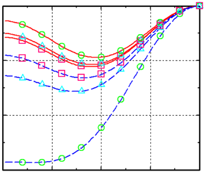
Figure 3 shows a comparison of the pressure coefficient $C_p^o$ with respect to $\theta$ between the present penalization results and the conventional analytical results of Bar-Lev & Yang (Reference Bar-Lev and Yang1975). In figure 3 the solid lines indicates the present penalization results of $C_p^0 = - 4 \sin ^2{\theta } - 4 \sqrt {\nu _o / ( {\rm \pi}T )} ( 1 - e^{- \lambda _o T} ) ( 1 + \cos {\theta } ) + O( \epsilon ^2 )$ whereas the dotted lines are the conventional results of Bar-Lev & Yang (Reference Bar-Lev and Yang1975) of $C_p^0 = - 4 \sin ^2{\theta } - 4 \sqrt {\nu _o / ( {\rm \pi}T )} ( 1 + \cos {\theta } ) + O( \epsilon ^2 )$. Here, $C_p^o$ means the pressure coefficient that is defined by the difference from the front point of the cylinder. It seems that the pressure distributions on the cylinder surface are in nice agreement with the conventional results for $\lambda _o \gg 1$.

Figure 3.

Comparison of the pressure coefficient $C_p^o$ at $\nu _o = 1$ against the conventional result of Bar-Lev & Yang (Reference Bar-Lev and Yang1975). In panel (a), the dashed lines are the results of Bar-Lev & Yang (Reference Bar-Lev and Yang1975).

Next, we will derive the drag coefficient $C_D$ using (3.53). Omitting the analysis, the final representation of $C_D$ is written as (see Appendix B for the detailed derivation)

(3.54)$$\begin{gather} C_D = 4 \sqrt{\frac{{\rm \pi} \nu_o}{T}} - \frac{3}{2 \lambda_o} \sqrt{\frac{{\rm \pi} \nu_o}{T^3}} \left( 1 - e^{- \lambda_o T} \right) + \frac{\rm \pi}{4} \frac{\lambda_o}{\epsilon} e^{- \lambda_o T / 2} \left[ I_0 \left( \frac{\lambda_o T}{2} \right) - I_2 \left( \frac{\lambda_o T}{2} \right) \right] \nonumber\\ + \epsilon \nu_o {\rm \pi}\left\{ 1 - e^{- \lambda_o T / 2} \left[ I_1 \left( \frac{\lambda_o T}{2} \right) + I_0 \left( \frac{\lambda_o T}{2} \right) \right] \right\}. \end{gather}$$

It can be found that (3.54) asymptotically exhibits 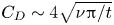$C_D \sim 4 \sqrt {\nu {\rm \pi}/ t}$ as $\lambda \to \infty$. As shown in Bar-Lev & Yang (Reference Bar-Lev and Yang1975), the friction drag is the same as the pressure drag for the first order in the case of $\lambda \to \infty$. Hence, since $\chi$ is zero in the fluid domain ${\mathscr F}$, there is the possibility that the pressure drag is not taken into account in (3.50) so that (3.51) exhibits the half-value of the results of Bar-Lev & Yang (Reference Bar-Lev and Yang1975) as $\lambda \to \infty$. This will be a future problem.

Furthermore, we will derive the drag coefficient $C_D$ using the alternative formula that is obtained from the hydrodynamic impulse (see Shiels Reference Shiels1998):

(3.55)\begin{equation} C_D ={-} \frac{{\textrm{d}}}{{\textrm{d}} t} \int_{\mathscr F} y \omega \, {\textrm{d}} V ={-} \frac{{\textrm{d}}}{{\textrm{d}} T} \int_0^{2 {\rm \pi}} \sin{\theta} \,{\textrm{d}} \theta \int_0^\infty \omega^i ( 1 + \epsilon R )^2 \,{\textrm{d}} R. \end{equation}

We here note that $T$ is stretched as $T = t / \epsilon$. Omitting the analysis, the final representation of $C_D$ is written as (see Appendix C for the detailed derivation)

(3.56)\begin{equation} C_D = 4 \sqrt{\frac{{\rm \pi} \nu_o}{T}} - \frac{5}{2 \lambda_o} \sqrt{\frac{{\rm \pi} \nu_o}{T^3}} \left( 1 - e^{- \lambda_o T} \right) - \frac{\rm \pi}{\epsilon} \frac{\lambda_o}{4} e^{- \lambda_o T / 2} \left[ I_2 \left( \frac{\lambda_o T}{2} \right) - I_0 \left( \frac{\lambda_o T}{2} \right) \right]. \end{equation}

As $\lambda _o \to \infty$, (3.56) behaves like

(3.57)\begin{equation} C_D \sim 4 \sqrt{\frac{{\rm \pi} \nu_o}{T}} + \frac{1}{\epsilon} \sqrt{\frac{\rm \pi}{\lambda_o T^3}} - \frac{5}{4 \lambda_o} \sqrt{\frac{{\rm \pi} \nu_o}{T^3}}. \end{equation}

It can be also found that the present penalization result converges to the same result, i.e. $C_D \sim 4\sqrt {{\rm \pi} \nu / t}$ of Bar-Lev & Yang (Reference Bar-Lev and Yang1975) as $\lambda \to \infty$. In (3.55), we note that the integral region is limited to the fluid region. Let us consider the case that the integral region is the inside of the cylinder, i.e. $( {\textrm {d}} / {\textrm {d}} t ) \int _{\mathscr B} y \omega \, {\textrm {d}} V$. Then, we have (see the detailed derivation in Appendix C)

(3.58)$$\begin{gather} \frac{{\textrm{d}}}{{\textrm{d}} t} \int_{{\mathscr B}} y \omega \, {\textrm{d}} V ={-}\frac{1}{\lambda_o} \sqrt{\frac{{\rm \pi} \nu_o}{T^3}} \left( 1 - e^{- \lambda_o T} \right) + 2\sqrt{\frac{\nu_o}{{\rm \pi} T}} e^{- \lambda_oT} + \frac{1}{2} \sqrt{\frac{{\rm \pi} \nu_o}{T^3}} e^{- \lambda_o T} \nonumber\\ + \sqrt{\frac{{\rm \pi} \nu_o}{T}} \lambda_o e^{- \lambda_o T} + \frac{\rm \pi}{8} \frac{\lambda_o}{\epsilon} e^{- \lambda_o T / 2} \left[ I_0 ( \lambda_o T / 2 ) - I_2 ( \lambda_o T / 2 ) \right]. \end{gather}$$

Thus, we can see that the first approximation of $C_D$ is derived from the fluid flow domain ${\mathscr F}$, since from the cylinder flow region ${\mathscr B}$ it is of the order of $1 / \sqrt {\lambda }$ as shown in the above equation. These results imply that the flow in the fluid region plays an important role in deriving the drag coefficient.

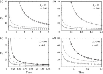
Figure 4 shows a comparison of $C_D$ at $\nu _o = 1$ between the present penalization result and the conventional result of Bar-Lev & Yang (Reference Bar-Lev and Yang1975) that is $C_D = 4 \sqrt {{\rm \pi} \nu _o / T} + {\rm \pi}\epsilon \nu _o ( 9 - 15 / \sqrt {{\rm \pi} } )$. Figure 4(a,b) are the results of $\epsilon = 0.01$ and figure 4(c,d) are of $\epsilon = 0.1$. In figure 4, the result plotted with circles is calculated by (3.51) that is obtained from the integration of the penalization term. The result plotted with triangles is calculated by (3.54) that is obtained from the integration of the vorticity and its derivative at $r = 1$. The results plotted with squares is calculated by (3.56) that is obtained from the hydrodynamic impulse. As observed, two results, except the integration of the penalization term plotted with circles, approach the conventional result of Bar-Lev & Yang (Reference Bar-Lev and Yang1975) with increasing $\lambda _o$. Furthermore, the results of both (3.54) and (3.56) are in nice agreement with each other and, therefore, the fluid flow can be found to be modelled well by the penalization method.

Figure 4.

Comparison of the drag coefficient $C_D$ at $\nu _o = 1$ between several formulae against the conventional result of Bar-Lev & Yang (Reference Bar-Lev and Yang1975). The symbols used are: circle, (3.51) that is obtained by the integration of the penalization term; triangle, (3.54) that is obtained by the integration of the vorticity and its derivative at $r = 1$; square, (3.56) that is obtained from the hydrodynamic impulse; dashed line, Bar-Lev & Yang (Reference Bar-Lev and Yang1975).