Introduction
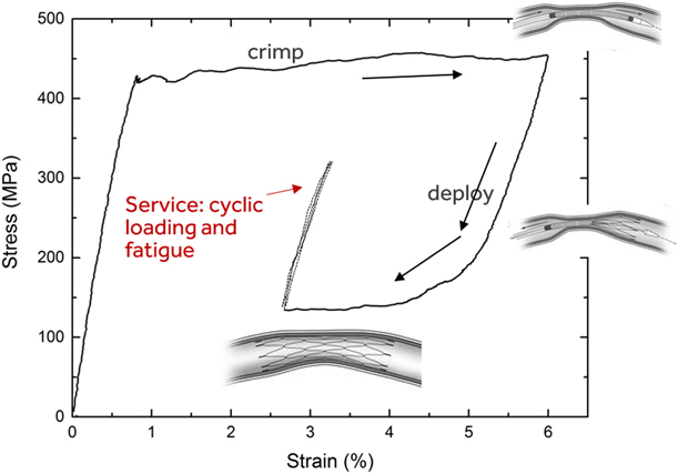
Superelastic Nitinol (Ti–50–51% Ni), owing to 6–8% recoverable strain from a reversible stress-induced martensitic transformation (SIMT), is widely used for fabrication of self-expandable biomedical implants such as stents and transcatheter heart valve frames. These devices are compressed and loaded into a small diameter catheter for minimally invasive delivery to the target anatomical location; upon deployment, the device self-expands and exerts the necessary force on the surrounding anatomy: e.g., keeping the artery open to restore blood flow. When the device is crimped into a catheter, high-stress regions undergo a two-stage SIMT: the parent B2 austenite phase transforms to a monoclinic B19′ martensite via an intermediate R-phase at the so-called upper plateau stress (UPS) (see Fig. 1). Because the transformation to B19′ rarely proceeds to completion, some R-phase and B2 may persist after SIMT. For simplicity, we will use the terms “martensite” and SIM to refer to this mixture, unless otherwise indicated. When the device is released from the catheter at the target location, the device partially recovers the strain through a spontaneous reverse transformation to austenite at the lower plateau stress (LPS). The device then exerts an outward force on the surrounding tissue to restore and maintain blood flow. So, the device design restricts it from being fully unloaded upon release from the catheter, leaving it in an austenite plus martensite mixed-phase state.
Schematic illustration of mechanical conditions experienced by a typical Nitinol medical device during crimping, deployment, and service.

During service as biomedical implants, Nitinol devices experience cyclic loading from cardiac cycles and musculoskeletal movements, often in the high-cycle fatigue regime. For instance, in the case of heart valve frames, 15 years of cardiac cycles equals 600 million cycles of loading. Therefore, understanding the fatigue behavior of Nitinol in a mixed-phase state is of significant importance. Given the small dimensions of stents and heart valve frames and the high crack growth rates in Nitinol [Reference McKelvey, Ritchie, Neenan, Marcolongo and Valentini1], if crack initiation occurs during service, fracture of struts is highly probable within a small fraction of the lifetime of the implant [Reference Robertson, Pelton and Ritchie2]. Accordingly, devices are typically designed using a strain–life approach so that the prevailing strain amplitudes are below the fatigue strength or threshold under those loading conditions; this fatigue threshold is defined as the maximum strain amplitude for which survival is ensured for a certain number of cycles depending on the application. The fatigue threshold may not be identical to the true endurance limit, if one exists; yet it is of great practical importance for device design. Within the context of biomedical implants such as stents and transcatheter heart valves, the fatigue threshold of Nitinol and its dependence on chemistry, microstructure, mechanical properties, and loading conditions are more relevant for device design and performance than crack growth characteristics.
Over the last three decades, a number of fundamental studies from a strain–life or stress–life perspective [Reference Melton and Mercier3, Reference Miyazaki, Sugaya and Otsuka4, Reference Kim and Miyazaki5, Reference Kim6, Reference Eggeler, Hornbogen, Yawny, Heckmann and Wagner7, Reference Wagner, Sawaguchi, Kausträter, Höffken and Eggeler8, Reference Bewerse, Gall, McFarland, Zhu and Brinson9, Reference Zheng, He and Moumni10] and from a crack growth standpoint [Reference McKelvey, Ritchie, Neenan, Marcolongo and Valentini1, Reference Robertson, Pelton and Ritchie2, Reference McKelvey and Ritchie11, Reference Robertson, Mehta, Peltonand and Ritchie12, Reference Daly, Miller, Ravichandran and Bhattacharya13, Reference Robertson and Ritchie14] have shed considerable light on Nitinol fatigue and helped guide medical device design. Robertson et al. [Reference Robertson, Pelton and Ritchie2, Reference Robertson and Ritchie14] and Pelton [Reference Pelton15] have summarized the present understanding of the subject as it is relevant to biomedical implants. We briefly summarize below relevant observations and discoveries made in prior work that are pertinent to the present article.
Melton and Mercier [Reference Melton and Mercier3] showed that repeated superelastic cycling, i.e., cyclic loading between zero load and through the SIM regime leads to fatigue fractures in 1000–10,000 cycles, and that because of the transformation stress plateaus, stress, and strain-controlled fatigue behavior are substantially different from one another. In rotary beam bending fatigue testing of cold-worked wires (i.e., zero mean strain), Miyazaki et al. [Reference Miyazaki, Mizukoshi, Ueki, Sakuma and Liu16] and Kim and Miyazaki [Reference Kim and Miyazaki5] showed that fatigue life of Nitinol is extended when it exists in a single phase (either austenite or martensite) compared with strain regimes where the stress-induced phase transformation occurs. Data from Reinoehl et al. [Reference Reinoehl, Bradley, Bouthot and Proft17], Sheriff et al. [Reference Sheriff, Pelton and Pruitt18], and Morgan et al. [Reference Morgan, Wick, DiCello and Graham19] show abrupt transitions in the strain amplitude–fatigue life or the ε-N curve that correlate with the SIMT. In a series of articles, Sawaguchi et al. [Reference Sawaguchi, Kausträter, Yawny, Wagner and Eggeler20], Wagner and Eggeler [Reference Wagner and Eggeler21], Eggeler et al. [Reference Eggeler, Hornbogen, Yawny, Heckmann and Wagner7], and Wagner et al. [Reference Wagner, Sawaguchi, Kausträter, Höffken and Eggeler8] have showed that rotary beam fatigue data fall into three regimes, one where SIM is active, one where it is inactive, and an intermediate region where local SIM is probable at stress raisers.
Though the abovementioned studies have provided considerable insight into Nitinol fatigue when the material is cycled from zero strain through the superelastic transformation, applying these insights to the case of a typical Nitinol medical device requires additional considerations. In the application, austenite and martensite coexist, and the mean or the starting strain is rarely zero. Tabanli et al. [Reference Tabanli, Simha and Berg22], Kugler et al. [Reference Kugler, Matson and Perry23], and others [Reference Robertson, Pelton and Ritchie2, Reference Pelton15] have pointed out the importance of nonzero mean strain conditions. Pelton et al. [Reference Pelton, Schroeder, Mitchell, Gong, Barney and Robertson24] and Robertson et al. [Reference Robertson, Launey, Shelley, Ong, Vien, Senthilnathan, Saffari, Schlegel and Pelton25] have since incorporated this key element into fatigue testing of stent subcomponents. These authors employed diamond-shaped specimens that are representative subcomponents of stents. To simulate the nonzero strain resulting from a stent being compressed into a catheter and being released into an artery, they compressed and partially unloaded the diamond-shaped specimen before cyclically loading it in displacement control. This approach is well suited to assessing the fatigue performance of device components and for comparing different material and processing conditions. However, because of the complex shape and gradients in stress and strain, understanding fundamental aspects of Nitinol fatigue in a mixed-phase condition with sufficient clarity is difficult with this approach. An approach to better characterize stress and strain distribution during cycling would be mixed-phase loading of a simpler specimen geometry such as a dog-bone specimen loaded in uniaxial tension. Although Pelton [Reference Pelton15] and Robertson et al. [Reference Robertson, Launey, Shelley, Ong, Vien, Senthilnathan, Saffari, Schlegel and Pelton25] have reported data from such experiments, a detailed analysis of the strain distribution, crack initiation location, etc., is not available in the published literature.
Under tensile loading, Nitinol undergoes strain localization: Luders band-like deformation fronts propagate during the SIMT [Reference Shaw and Kyriakides26, Reference Leo, Shield and Bruno27]. In a mixed-phase state, the specimen is split into macroscopic domains of martensite and austenite separated by phase boundaries. The impact of strain localization and heterogeneous strain distribution on monotonic loading has been investigated thoroughly [Reference Bewerse, Gall, McFarland, Zhu and Brinson9, Reference Daly, Ravichandran and Bhattacharya28, Reference Reedlunn, Churchill, Nelson, Shaw and Daly29] using strain mapping and digital image correlation (DIC). Crack-tip deformation during cyclic loading has similarly been investigated using DIC [Reference Daly, Miller, Ravichandran and Bhattacharya13]. However, crack initiation during cyclic loading has not received sufficient interest, the exception being a recent publication by Zheng et al. [Reference Zheng, He and Moumni10]. These authors used DIC to investigate low-cycle fatigue behavior and failure in tension under stress-controlled transformation cycling and found that fatigue failures occurred in what they refer to as “active zones” where cyclic SIMT takes place. However, under stress-control, there are several such “active zones” along the gage section, whose number changes from cycle to cycle as does the strain amplitude in each location. It is therefore not clear why a specific “active zone” is particularly prone to failure. Although this previous work [Reference Zheng, He and Moumni10] adds to the understanding of Nitinol fatigue in general, it does not adequately address the role of strain localization during displacement-controlled loading in the mixed-phase case and its impact on fatigue behavior and the fatigue threshold, both of which are critically relevant to medical implants.
Thus, although there is considerable literature devoted to understanding the fundamental aspects of Nitinol fatigue, the focus has rarely been on fatigue in the mixed-phase composite that is the most common scenario encountered in applications of Nitinol in medical devices. Still, based on data from some of these studies that show some correlation between low-cycle fatigue failures and activating the phase transformation [Reference Melton and Mercier3, Reference Eggeler, Hornbogen, Yawny, Heckmann and Wagner7, Reference Wagner, Sawaguchi, Kausträter, Höffken and Eggeler8, Reference Zheng, He and Moumni10], it is reasonable to expect this to hold true for mixed-phase loading as well. Often, fatigue data are bimodal: with decreasing strain amplitude, low-cycle failures transition abruptly into high-cycle runouts, which suggests that the low-cycle fatigue threshold is the same as the high-cycle fatigue threshold. If this hypothesis is correct, it would serve as a useful tool for material selection and component design. One could predict the fatigue threshold from the operating stresses and the plateau stresses, all of which can be determined without running a fatigue test to failure. However, experimental data are not available in the published literature to confirm this hypothesis. It is also unclear whether fatigue cracks would initiate in the martensite or austenite when a mixed-phase mixture is cyclically loaded. It seems reasonable to expect failure at the austenite–martensite interface where forward and reverse transformation could take place; yet this has not been shown conclusively.
A related aspect is rate dependence in cyclical mechanical response, which is of importance, given the widespread use of accelerated fatigue testing of Nitinol components, often performed at frequencies of 50–60 Hz in a temperature-controlled water-based medium. Shaw and Kyriakides [Reference Shaw and Kyriakides26] showed that even in a temperature-controlled water bath, adiabatic self-heating and the consequent rate dependence are present. We can therefore expect rate dependence in the cyclic mechanical response during fatigue testing, if not in the fatigue life. This is relevant, given that the fatigue performance comparisons between different components and between material grades are done on the basis of mean and alternating strains, both of which are estimated from finite element models [Reference Pelton, Schroeder, Mitchell, Gong, Barney and Robertson24, Reference Pelton, Gong, Duerig and Shrivastava30] that use quasi-static response to predict cyclic strains. To the best of our knowledge, the cyclic mechanical response in water has not been investigated for the mixed-phase state, specifically for displacement-controlled loading.
The objective of the present study is to address gaps in understanding of fatigue of mixed-phase Nitinol, relevant to medical implant applications. Specifically, the following questions are addressed in the present study.
(i) How is strain partitioned during cyclic loading in the mixed-phase state? What is the significance of strain localization to metrics that characterize fatigue in tension?
(ii) Is cyclic mechanical response rate dependent in water?
(iii) During fatigue loading of a mixed-phase composite, where does fatigue crack initiation occur?
(iv) Are the phase transformation threshold and the fatigue threshold linked for mixed-phase loading? In other words, would activation of the SIM lead to fatigue failures?
We performed a series of tension–tension cyclic loading experiments and fatigue tests (cyclic loading to 10 million cycles or to failure, whichever came first) on Nitinol dog-bones in the mixed-phase state. Prior work has shown that uniaxial tension of a uniform cross-section leads to the stochastic nucleation of multiple martensitic bands within the gage section [Reference Zheng, He and Moumni10, Reference Daly, Ravichandran and Bhattacharya28]. This presents a challenge for following strain and damage evolution within the specimen. We circumvented this by including a taper in the center of the dog bone which ensures preferential nucleation of a single martensitic band at the narrowest portion of the gage section without causing significant stress concentration or stress gradients. This enabled more systematic observations and greatly enhanced our understanding of cyclic mechanical response.
We used DIC and high-speed video recording to track cyclic strain distribution and localization as well as crack initiation. Three different loading frequencies were used to investigate rate effects in cyclic loading. Some tests were performed in water to understand the efficacy of water in suppressing rate dependence. Fatigue tests were done to identify the fatigue threshold for low-cycle fatigue and its relationship to the stress-induced phase transformation and the monotonic stress–strain response.
Experimental procedure
Material and specimen fabrication
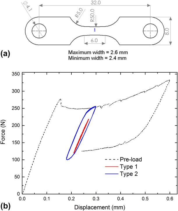
A 0.25 mm thick superelastic 55.9 wt% Ni Nitinol sheet was purchased from Johnson-Matthey, San Jose, California. As per the manufacturer’s certificate, the active A f is 13.4–14.5 °C. Dog bone–shaped specimens [see Fig. 2(a) for geometry] were laser cut from the sheet, microblasted, and electropolished to remove the recast and heat-affected material (∼25 μm) by Laserage Technology Corporation, Waukegan, Illinois, resulting in a smooth and brightly reflective surface finish. A slight taper is included in the gage section to facilitate the nucleation of a single martensitic band in the center of the gage section during tensile loading. The gage section profile has a radius of 50 mm. At band nucleation, the applied stress at the widest portion of the cross-section is only 8% smaller.
(a) Dog bone specimen geometry—all dimensions shown in millimeters. (b) Tensile force–displacement curves for the tapered dog bone specimens used in this study. The preload and Types 1 and 2 cyclic loading profiles are shown.

Displacement-controlled quasi-static tensile loading, cyclic loading, and fatigue testing
An MTS servohydraulic test frame with a 5 kN load cell was used throughout the study. All quasi-static tensile loading was conducted at a nominal strain rate of 10−4 s−1 to prevent adiabatic heating from latent heat release associated with the SIMT. Specimens were bolted to the tensile test fixtures. A compressed air jet was used to prevent specimen heating. All tests were performed at room temperature 23 ± 2 °C. Some tests were performed in a circulating water bath maintained at room temperature.
For all cyclic loading experiments and fatigue tests, a preloading procedure was applied that simulated the mechanical history of a typical implant, i.e., crimping the stent into a microcatheter and subsequent deployment at the location of interest. This involved a tensile displacement of 0.6 mm being applied until the entire gage section was transformed to martensite (approximately 6% average strain), followed by partial unloading to a displacement of 0.24 mm along the lower stress plateau so that a single band of martensite remained within a portion of the gage section. The average strain at this stage was approximately 3%. Subsequently, displacement-controlled sinusoidal load cycles were applied. Thus, the gage section of the dog-bone specimen is in a mixed-phase state (a central band of martensite flanked by austenite) for the duration of the cyclic test. The central band will likely contain a mixture of B19′, a small amount of R-phase and retained austenite. Similarly, in regions near and outside the band, some R-phase is expected to coexist with austenite. For simplicity, we will continue to refer to this as the “austenitic region”.
After conclusion of the test, the load–displacement data from the preloading curve were used to calculate the LPS, (σlps) and UPS (σups); the cyclic load–displacement data were used to calculate the nominal cyclic minimum stress (σmin) and the cyclic maximum (σmax) stress. The load corresponding to the cyclic displacement minimum applied in the test was read from the preloading portion of the load–displacement data, which was then divided by the minimum cross-sectional area within the gage section to calculate the LPS, σlps. Likewise, the load on the upper plateau corresponding to the applied cyclic displacement maximum was used to calculate the UPS, σups. The cyclic load data were fit to a sinusoidal curve to calculate the resultant cyclic maximum and minimum loads. These were divided by the minimum cross-sectional area to yield the σmax and σmin, respectively. If the cyclic response is identical to that of the quasi-static response, then σmin should equal σlps and σmax should equal σups.
Cyclic loading from the lower stress plateau can be categorized into Type 1 and Type 2, and both are illustrated in Fig. 2(b). In Type 1 loading, the applied displacement amplitude is such that the resultant stress range is smaller than the stress hysteresis, the difference between the forward and reverse transformation stresses (Δσ = σmax − σmin < σups − σlps). In this situation, transformation from austenite (and R-phase) to B19′ is not favored macroscopically. But the austenite to R-phase transformation could still occur; so, the deformation is not strictly elastic and will likely have an anelastic component. Deformation of the martensite is also likely to have an anelastic component due to movement of boundaries between variants. Hereafter, for simplicity of nomenclature, we will refer to this as “nominally elastic” deformation. No macroscopic movement of the phase boundary or changes in B19′ volume fraction are expected. In contrast, in Type 2 loading, the displacement amplitude is large enough to provide a driving force for forward and reverse SIMT. So, the volume fractions of austenite and B19′ could change through the course of each load cycle which, in this case, means that the single band can expand and contract along the gage section during cycling—i.e., the austenite–martensite interface will migrate back and forth. Thus, cyclic strain accommodation mechanisms and, by extension, fatigue damage mechanisms for Type 1 and Type 2 loading are anticipated to be different.
Each of three specimens, S1, S2, and S3, was preloaded to the LPS as described above and was subjected to Type 1 and Type 2 loading in succession at three different loading rates that are described in detail below. Surface events on specimen S1 were recorded using a high-speed digital camera during the cyclic loading portion of the test. A speckle coating was applied to the surface of S2 and images were acquired for DIC analysis. S3 was tested in water at room temperature.
(i) Type 1—displacement amplitude 30 µm;
(a) 0.004 Hz (approximately equivalent to 10−4 s−1 strain rate); 4–5 cycles
(b) 1 Hz (similar loading rate as cardiac cycles); 4–6 cycles
(c) 40 Hz (accelerated fatigue testing for material evaluation)—1000–2000 cycles
(ii) Type 2—displacement amplitude 60 µm;
(a) 0.004 Hz (approximately equivalent to 10−4 s−1 strain rate); 4–5 cycles
(b) 1 Hz (similar loading rate as cardiac cycles); 4–6 cycles
(c) 40 Hz (accelerated fatigue testing for material evaluation)—1000–2000 cycles
At 40 Hz, the proportional gain needed adjustment to stabilize the cyclic amplitude in the initial stage of the experiment. Since this process required a few seconds (first few hundred cycles), meaningful data and DIC analysis could be performed only on later cycles after making certain the intended displacement amplitude was attained. Hence, it was necessary to apply 1000–2000 cycles for the full experiment.
In addition, a strain–life diagram was obtained by testing several specimens, each at a single displacement amplitude and frequency until failure or until 10 million cycles. Some specimens were imaged during the test to determine the crack-initiation location.
Digital image correlation and surface imaging
DIC was used to obtain surface strain maps to follow strain distribution and strain localization within the gage section for both monotonic and cyclic loading. These specimens were speckle-coated with spray paint to facilitate DIC. The specimen surface was photographed at intervals by a Photron FastCam high-speed digital camera. For the slowest tensile and cyclic loading (0.004 Hz), one image was acquired every 2 s. For cyclic loading frequencies of 1 Hz and 40 Hz, the image acquisition rates were 125 and 5000 frames per second, respectively. For tracking, the phase boundaries and fatigue crack initiation events, the same acquisition rates were used on other specimens without the speckle coating.
DIC analysis was performed using the GOM Correlate Professional™ software to obtain surface strain maps. Strain–time histories were extracted from these strain maps for several points along a line parallel to the tensile axis and running through the mid-section of the specimen, sampling the central martensitic region and the two austenitic (or R-phase) regions that flank it, and that together comprise the gage section. For slow strain rate testing and for 1 Hz frequency, the tensile data and DIC image data were synchronized. Nominal stress (Force/initial cross section area at the midsection) versus local strain plots were generated for cases where such synchronization was successful. In addition to local strain, an average strain along the gage section was computed by selecting two points on the vertical midsection and calculating strain by measuring their separation distance.
A fourth specimen, S4, was used to find a correlation between applied displacement and resultant strain and strain amplitudes. The specimen was taken through the preloading procedure (load to 0.6 mm and unload to 0.24 mm) after which a series of strain amplitudes between 10 and 55 μm were applied in succession at 40 Hz.
Results
Type 1 cyclic loading—strain distribution
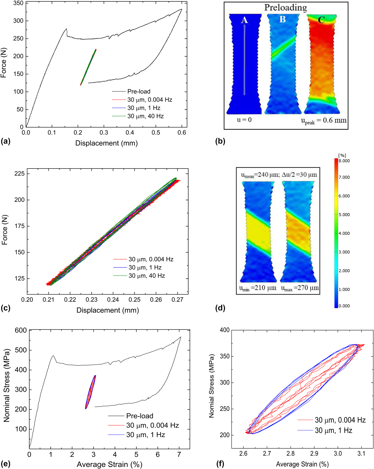
Figure 3(a) shows the load–displacement curves for preloading and Type 1 cyclic loading in air with compressed air cooling for specimen S2. Figure 3(b) shows extensional strain contours obtained by DIC analysis for the preload portion of this test: zero load, initiation of martensitic transformation, and peak displacement of 0.6 mm. During the preloading procedure, a single macroscopic martensitic band forms [Fig. 3(b)], made possible by the small taper in the gage section. As the displacement is increased to the maximum [from B to C in Fig. 3(a)], the martensitic band grows to encompass the entire gage section [Fig. 3(b)]. The positive slope in the load–displacement curve during the transformation to martensite in Fig. 3(a) is due to the taper in the cross-section. As the band progressively grows into wider cross-section, larger forces are required to reach the UPS. When the specimen is partially unloaded, the martensite band recedes toward the center of the specimen, and just prior to cyclic loading, there is one continuous macroscopic band of martensite within the gage section flanked on both sides by austenite.
Mechanical response during Type 1 loading. (a) Force–displacement curve for specimen S2 during Type 1 loading at 30 µm displacement amplitude. (b) Surface strain maps obtained by DIC during the preloading procedure at points A, B, and C marked on the force–displacement curve in (a). (c) Magnified view of only the cyclic portion of the force–displacement curve—note the insensitivity to cyclic frequency. (d) DIC strain maps at displacement minimum and maximum during cycling showing no observable change in martensite volume fraction. (e) Nominal stress–strain curves derived from load and DIC strain maps for 0.004 and 1 Hz. (f) Magnified view of the cyclic portion of the stress–strain curve in (e).

The cyclic loading curves for the three frequencies shown in Fig. 3(a) are enlarged in Fig. 3(c). There is no noticeable effect of the loading frequency, and the deformation appears to be nominally elastic. Strain maps at the minimum and maximum applied cyclic displacement are shown in Fig. 3(d) where we see no recognizable changes in the martensite volume fraction as represented by the bandwidth in the loading direction. Based on prior work [Reference Shaw and Kyriakides26] that shows the rate dependence to be a consequence of phase transformation (adiabatic heating from latent heat release), the lack of loading frequency dependence in Type 1 loading is expected, and is verified in Figs. 3(a) and 3(c).
From DIC, an average strain was computed for the gage section by measuring the change in length between two points along the midsection. A nominal stress was computed from the force using the initial cross-sectional area at the narrowest portion in the specimen. From these, a stress–strain curve was computed for the preload segment and for the cyclic loading at 0.004 and 1 Hz. These results are shown in Figs. 3(e) and 3(f). Because of the lack of synchronization between the load data (MTS tester) and strain data (camera-acquired images), a stress–strain plot was not computed for the 40 Hz cyclic loading.
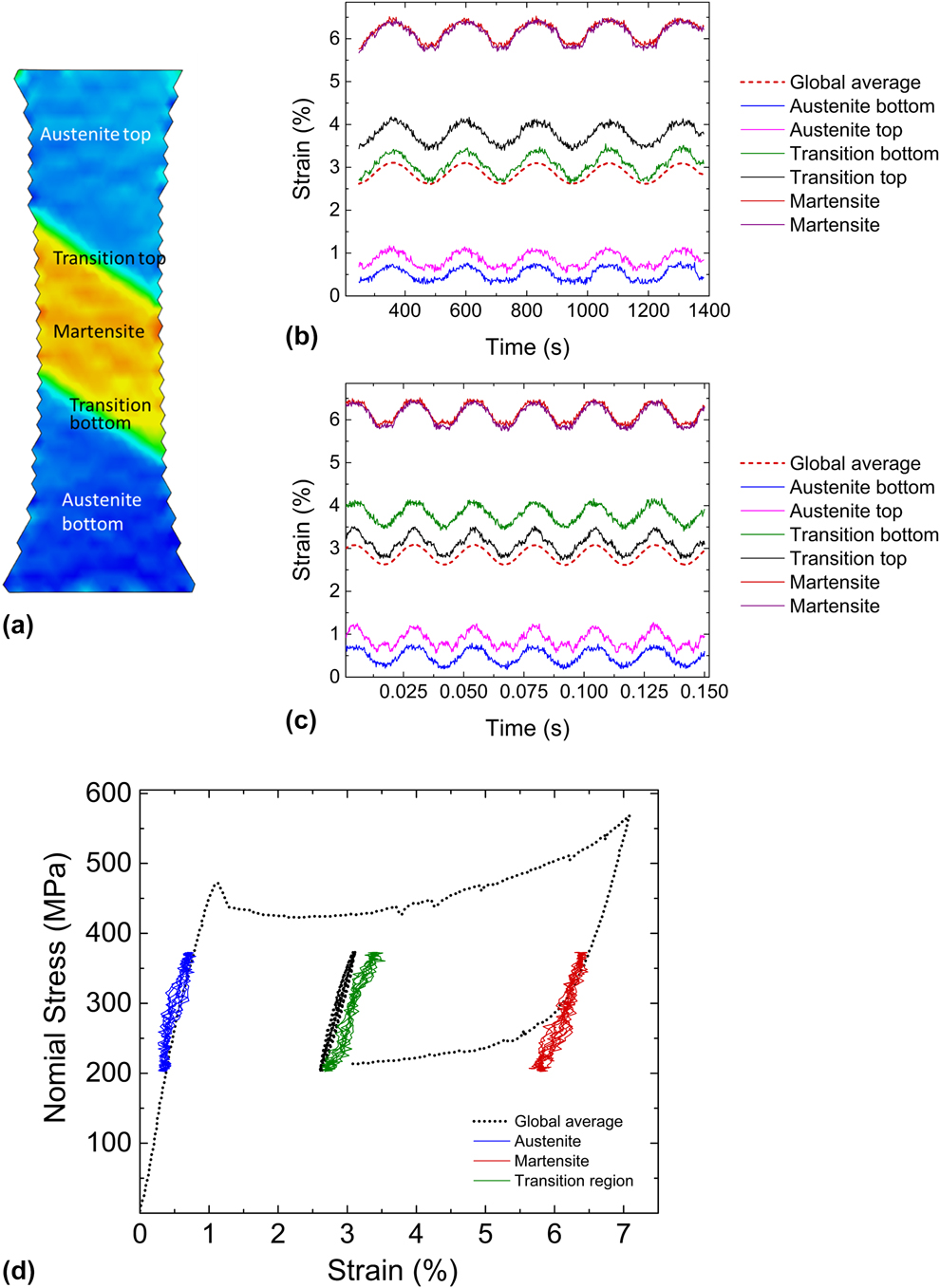
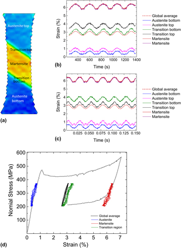
Figures 4(a)–4(d) show various aspects of strain distribution in S2 obtained by DIC analysis. Local strains were obtained from specific locations along the vertical axis of symmetry within the central martensitic band, the austenitic regions on the top and bottom, and the two transition regions sandwiched between the austenite and martensite [Fig. 4(a)]. Figures 4(b) and 4(c) show time histories of local strain during cyclic loading for the slowest and the fastest loading rates, along with the history of average strain. The martensitic region experiences a “mean strain” of nearly 6%, whereas the austenitic regions are well under 1% mean strain. By contrast, the mean strain based on an average strain measurement for the entire gage section is near 3%. The differences in local strain amplitudes across the gage section are not as large. The martensitic region undergoes a slightly larger strain amplitude than its austenitic counterparts, presumably because of its lower effective modulus as well as the taper which leads to slightly larger stresses in the martensitic region.
Strain distribution across the gage section for specimen S2 for Type 1 loading—same experiment as in Fig. 3. (a) Strain map at approximately mean displacement. (b) and (c) Local strain history from regions within the martensite, austenite, top and bottom transition zones [indicated in (a)], all compared with the global average for the lowest and the highest cyclic frequencies, respectively. (d) Local cyclic stress–strain curves obtained from DIC compared with the global average.

Thus, in Type 1 cyclic loading, the specimen behaves effectively as a macroscopic composite where each phase undergoes nominally elastic loading. At the macroscopic length scale, no further phase transformation to martensite is evident either in DIC-based strain analysis or in the load–displacement behavior. This can also be recognized in stress–strain space by superimposing point-wise stress–strain curves for the cyclic portion of the test (austenite, martensite, transition zone, and global average) on the overall complete loading–unloading stress–strain curve [see Fig. 4(d)]. The region that starts off as austenite cycles in the pretransformation pseudo-linear region of the stress–strain curve, whereas the martensitic region cycles at the right edge of the lower plateau.
Between what are clearly austenitic and martensitic regions, there is a 150–200 µm transition zone, which is distinct from a typical phase boundary, because phase boundaries are at most only a few atomic layers thick. From DIC analysis, the average strain within this zone is 3–4%, which falls between the austenite and martensite strains of <1% and >5%, respectively. This suggests that this zone is likely a mixture of austenite and martensite. The intermediate strain values are the result of averaging strain from the two phases that coexist and the lack of spatial resolution at the appropriate length scale to isolate strains associated with the individual phases in this zone.
Type 2 cyclic loading—strain distribution
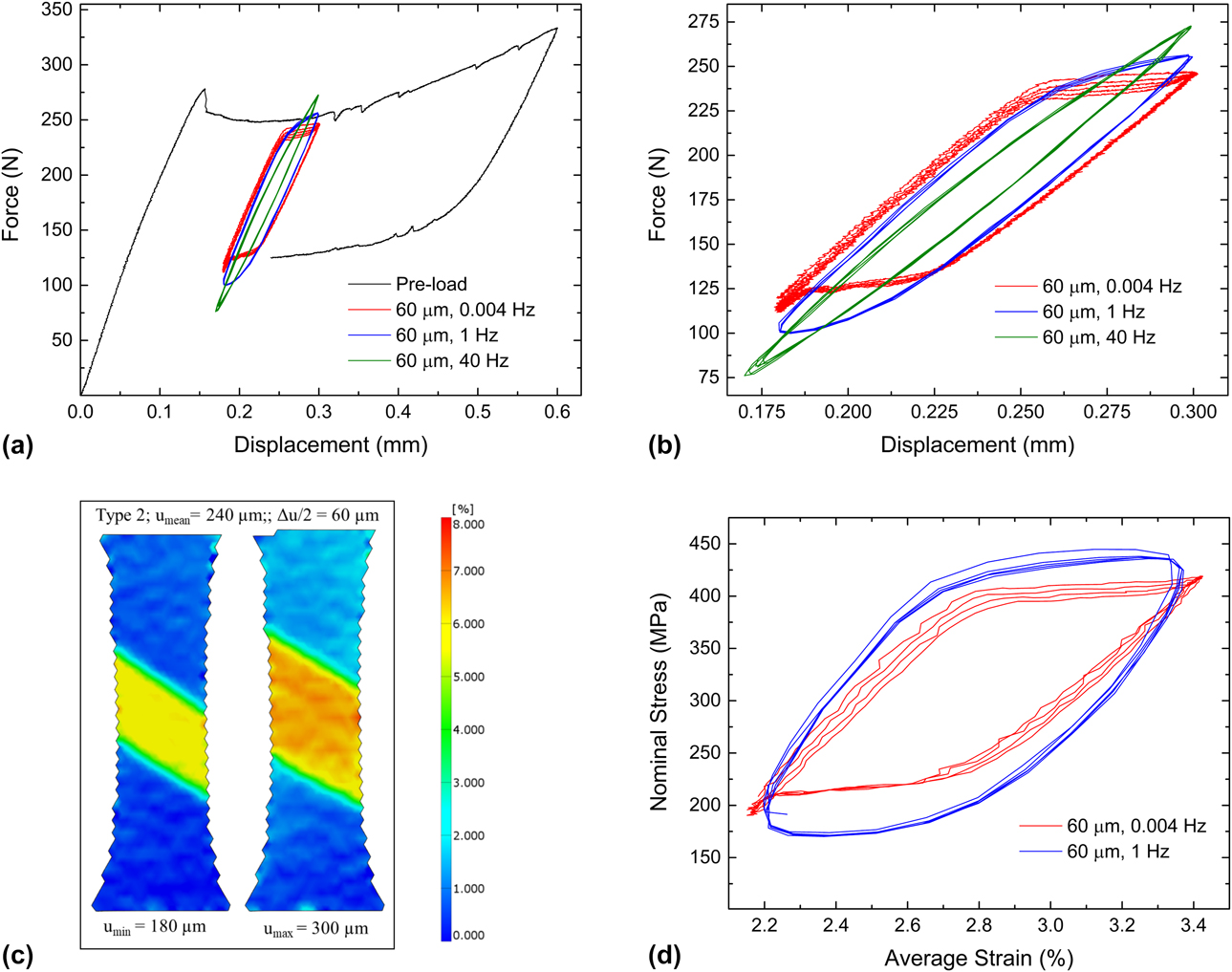
Following Type 1 loading, without unloading and re-applying the preloading, the same specimen S2 was loaded according to the Type 2 profile. A displacement amplitude of 60 µm was applied at three different frequencies 0.004, 1, and 40 Hz in succession. Load–displacement curves for these segments are shown in Fig. 5(a). Since preloading is not repeated for the Type 2 portion of the experiment, the preloading curve from Fig. 3(a) is referenced in Fig. 5. An enlargement of the cyclic portion is provided in Fig. 5(b). Unlike in Type 1 loading [Fig. 3(c)], the cyclic load–displacement curves show hysteresis corresponding to the forward and reverse austenite–martensite phase transformation; the mid-width and force maximum and minimum for these loops are rate dependent. In Fig. 5(c), surface strain maps corresponding to the displacement minimum and maximum for 0.004 Hz are shown, where a change in martensite volume fraction is evident, i.e., SIMT occurs in Type 2 cyclic loading. This is consistent with the load–displacement curves. The average strain for the cyclic portion was obtained from DIC analysis for the 0.004 Hz and 1 Hz cases and is plotted against the nominal stress in Fig. 5(d). For the 0.004 Hz case, although a total of 5 cycles are shown in the load–displacement curves, only four cycles were recorded in images for DIC analysis. A loading frequency dependence is evident in Figs. 5(a), 5(b), and 5(d). For the same applied displacement amplitude, with increasing frequency, the nominal stress range increases.
Mechanical response during Type 2 loading. (a) Force–displacement curves for specimen S2 during preloading and cyclic loading at a displacement amplitude of 60 µm. (b) Magnified view of the cyclic portion of the curve in (a). (c) Surface strain maps obtained by DIC at cyclic displacement minimum and maximum for 0.004 Hz—note the significant change in martensite volume fraction. (d) Nominal cyclic stress–strain curves corresponding to force–displacement curves in (b) for 0.004 and 1 Hz.

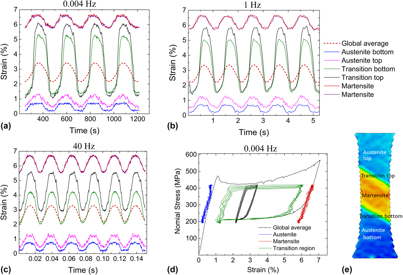
Figures 6(a)–6(c) show local strain histories in the tensile specimen along the vertical midsection (obtained from DIC) for all three loading frequencies. Specifically, strain histories in the central martensite band, in the austenite regions above and below it, and in the two transition zones sandwiched in between are presented in these figures [these zones are identified in Fig. 6(e)]. In each of these figures, the average strain history is also shown. Regions that are well within the austenitic and martensitic domains underwent nominally elastic cycling with strain amplitudes not much larger than those seen in Type 1 loading [see Figs. 4(b) and 4(c)], despite the fact that the displacement amplitude for Type 2 is double that of Type 1. By contrast, the transition zones experience strain amplitudes two to four times the average. Thus, for a given loading frequency, the majority of the additional imposed cyclic displacement amplitude beyond what constitutes the limit of Type 1 displacement is apparently accommodated by these transition zones. In Type 2, the mean strain and the strain amplitude vary significantly across the gage section.
Strain distribution for Type 2 loading for specimen S2. Local strain history from regions within the martensite, austenite, top and bottom transition regions [locations indicated in (e)], all compared to the global average for (a) 0.004 Hz, (b) 1 Hz, and (c) 40 Hz. (d) Local stress–strain curves for 0.004 Hz frequency compared against the global average. (e) Strain map at displacement maximum for reference.

The frequency-dependent mechanical response observed in Figs. 5(a), 5(b), and 5(d) is elucidated in the strain-time history plots in Figs. 6(a)–6(c). As the frequency increases, the strain amplitude experienced by the transition region decreases. Since the total displacement amplitude does not change with frequency, this decrease is offset by increases in both the austenite and the martensitic regions, more so in the martensite due to its lower modulus. Thus, both global and local data indicate that phase transformation is retarded at higher loading frequencies. Shaw and Kyriakides [Reference Shaw and Kyriakides26] have shown that for monotonic tensile loading, higher strain rates result in adiabatic heating which causes progressively increasing transformation stresses as per the Claussius–Clayperon relation (dσ/dT = −ΔH/(εT)). Thus, phase transformation is more difficult to sustain at higher loading rates. Our observations confirm that this holds true during cyclic response. Consequently, at higher frequencies, a greater fraction of the applied displacement amplitude is borne by the austenitic and martensitic regions.
Surface observations during cyclic loading and fatigue damage initiation
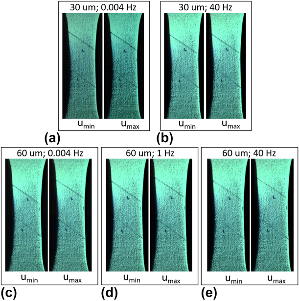
Specimen S1 was loaded in an identical manner to S2. The principal difference was that the specimen surface was imaged without a speckle coating, using the same camera and acquisition rates used for specimen S2. Two marks were made with a pen on the specimen surface to visually track the movement of the austenite–martensite boundary during the experiment; these marks can be seen in Fig. 7. To obtain quantitative information of boundary movement during cycling, high-speed camera images at maximum and minimum displacement were compared and the results are described below.
Snapshots of the surface of specimen S1 at displacement minima and maxima during cyclic loading for both Type 1 and Type 2 cases. Frequency and displacement amplitude are indicated above each set of figures. In all figures, the austenite–martensite phase boundary is clearly visible. Reference ink marks were made to locate the phase boundary and follow its movement. Although there is little noticeable boundary motion in Type 1 (30 µm), the boundary migrates across macroscopic distances during Type 2 loading (60 µm) for all frequencies.

Images taken approximately at the displacement minima and maxima for Type 1 loading (30 µm displacement amplitude) at 0.004 Hz and 40 Hz are shown in Figs. 7(a) and 7(b), respectively. The two austenite-martensite boundaries are clearly visible as relief lines on the surface at ∼34° to the horizontal. During cycling, the boundaries essentially remain stationary [compare Figs. 7(a) with 7(b)]. This is consistent with the findings presented in section “Type 1 cyclic loading—strain distribution”: In Type 1 loading, there is no appreciable phase transformation during cyclic loading.
Figures 7(c)–7(e) show similar surface images during Type 2 loading (60 µm displacement amplitude) at the displacement minima and maxima for 0.004, 1, and 40 Hz, respectively. In all three cases, there is a clear shift in boundary positions identified by the relief lines. Specifically, the change in the width of the martensitic band between U max and U min is 730 µm, 620 µm, and 320 µm for 0.004, 1, and 40 Hz, respectively. That is, in Type 2 cyclic loading, forward and reverse transformation occurs across a small portion of the gage section and the boundary moves farther at the lowest frequency. This implies that the change in martensite volume fraction per cycle is sensitive to cycling frequency in a manner consistent with the response observed in the load–displacement curves. Again, this observation is in agreement with the observations in 3.2 as well as with those of Shaw and Kyriakides [Reference Shaw and Kyriakides26].
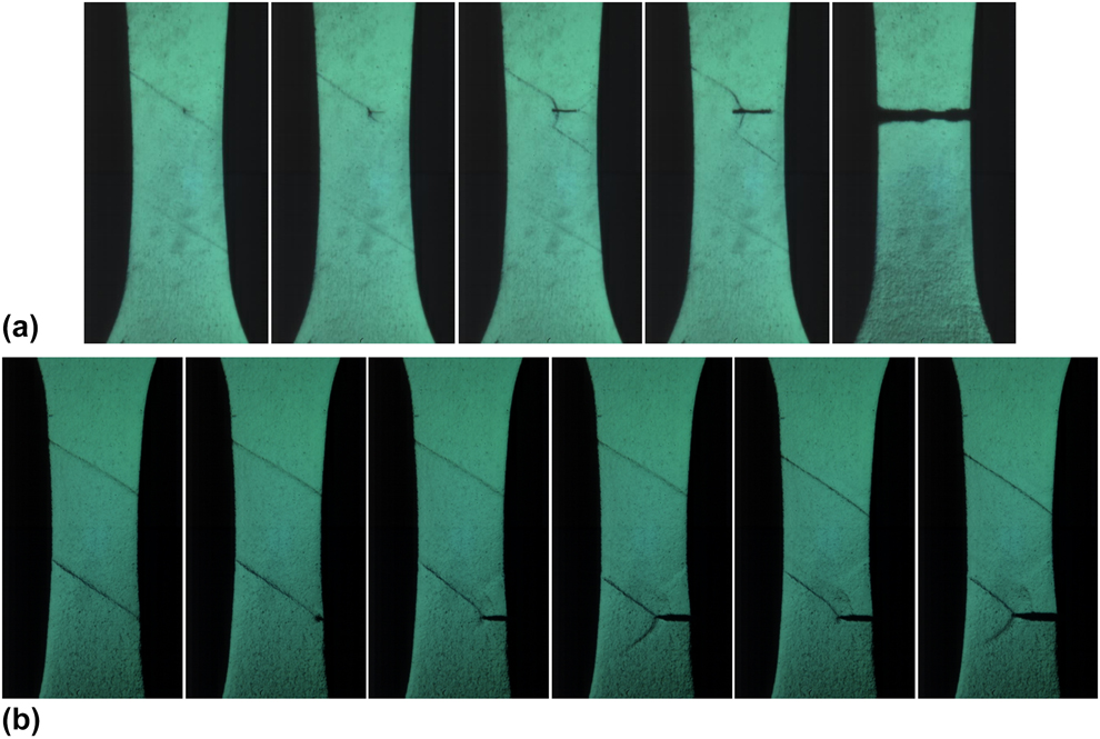
Two specimens, S5 and S6, were cycled to failure following the preloading procedure, and at a displacement amplitude of 60 µm at 40 Hz and 1 Hz, respectively; the specimen surface was continuously imaged and recorded using a high-speed camera. In both cases, a fatigue crack initiated in the austenite–martensite transition zone and propagated to failure perpendicular to the loading axis [Figs. 8(a) and 8(b)]. After crack initiation was observed on the specimen surface, crack propagation to failure occurred in less than 200 cycles which is less than 5% of the total fatigue life. In S5, a crack appeared on the flat surface of the specimen away from the edges on the upper transition region [Fig. 8(a)], whereas in S6, it initiated at the right edge on the bottom transition zone [Fig. 8(b)]. In S5 [Fig. 8(a)], the crack appears to extend more readily into the austenite than into the martensite with the effect of partial unloading below the crack and the reversion of martensite to austenite. On the austenitic side, ahead of the crack front, the stress concentration associated with the crack tip appears to convert austenite to martensite—see arrows in Fig. 8(a). In S6 [Fig. 8(b)], the crack initiated at the specimen edge and at the transition zone. As it advances, the transition zone seems to extend along with the crack tip, continually providing a crack growth path. In addition, a narrow band of martensite running diagonally from the bottom tip of the crack appeared and disappeared during crack growth, indicating cyclic phase transformation ahead of the crack tip. Previously, Ungar et al. [Reference Ungár, Frenzel, Gollerthan, Ribárik, Balogh and Eggeler31] indirectly observed this phenomenon using X-ray diffraction. It is unclear from these images if the region immediately ahead of the crack tip into which the crack grows remains austenitic (or in R-phase) or if it transforms to martensite. Last, it is noted that the crack does not initiate at the center of the gage section where the nominal principal stress is the highest.
Crack initiation at the austenite–martensite transition zone for Type 2 loading at a displacement amplitude of 60 µm. (a) Specimen S5 loaded at 40 Hz. (b) S6 loaded at 1 Hz.
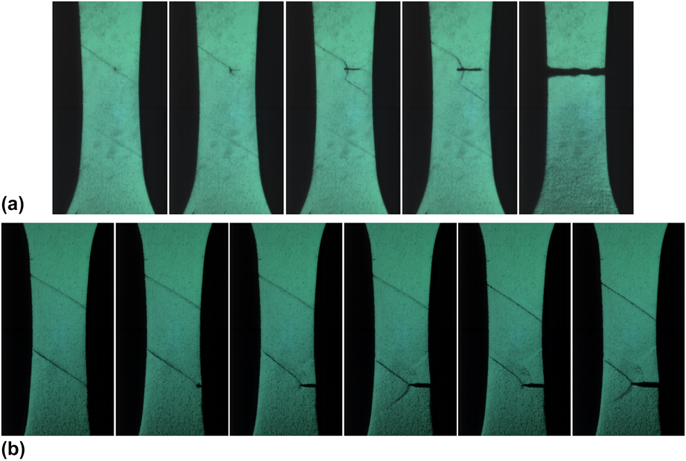
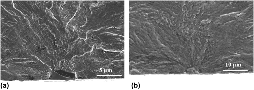
Another specimen, S7, tested to failure at a displacement amplitude of 55 µm at 40 Hz, also fractured by initiation in the transition region (not shown here). To date, all specimens tested to failure that were observed by a camera in situ failed by crack initiation at/near the transition region. Figure 9 shows two representative fractographs where in each instance, a near-surface inclusion is present at the initiation site, consistent with prior observations [Reference Robertson, Pelton and Ritchie2]. Based on these observations, it is evident that fatigue crack initiation occurs at an inclusion that is located at or near the transition zone.
Representative fractographs of fatigue failures each showing an inclusion at the initiation site.

Effect of testing medium
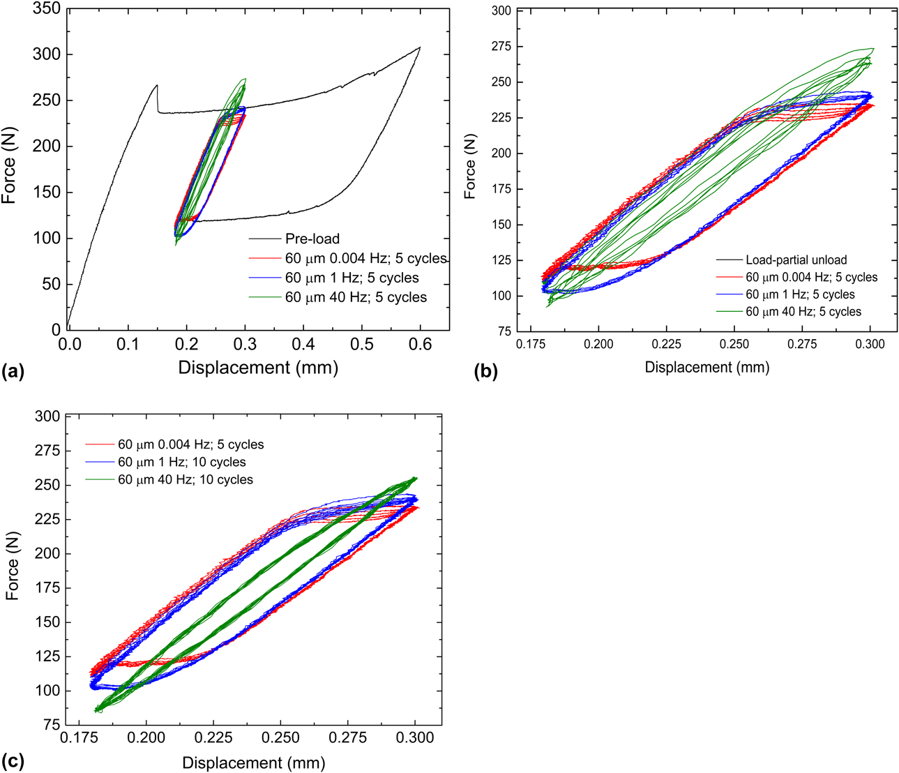
Specimen S3 was tested in the same manner as S2, but in water maintained at room temperature. In S2, for Type 1 loading, no significant frequency effects were observed. For Type 2 however, there was a clear loading frequency dependence: at higher frequencies, the volume of material undergoing cyclic SIMT was smaller than that observed at the lower frequencies. The same holds true for S3 tested in water. Figure 10 shows the load–displacement curves for Type 2 cyclic loading, which are similar to those for S2 (Fig. 5). For the 40 Hz case, at least 1000 cycles were applied. In this instance, the proportional gain did not require adjustment for 40 Hz loading and therefore the data from the first few cycles are valid and shown in Figs. 10(a) and 10(b): The load decreases progressively with increasing cycle number as expected. In Fig. 10(c), the last few cycles are shown for the 40 Hz loading, by which time the load–displacement curves have stabilized. Comparison of the response of S3 to the response of S2 shows no substantial difference in cyclic mechanical response between tests conducted in water and those conducted in air in the first few to few thousand cycles.
Cyclic mechanical response and frequency dependence in water. (a) Force–displacement curves for Type 2 loading of specimen S3 (60 µm displacement amplitude) along with pre-loading. All load cycles from 0.004 Hz, the first 5 load cycles for 1 Hz and 40 Hz loadings are shown. (b) Magnified view of the cyclic loading curves in (a). (c) cyclic loading curves after stabilization of load cycles at 40 Hz: 10 cycles toward the end of the loading experiment for 40 Hz are shown along with all load cycles from 1 Hz to 0.004 Hz loading.

Fatigue life data
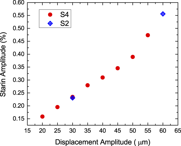
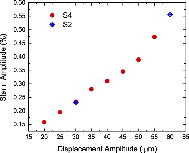
A total of 27 specimens were fatigue tested at 40 Hz following the prestraining procedure described previously in Sections “Experimental procedure” and “Results”. Eighteen of these were tested in air at room temperature with compressed air cooling; the remaining nine were tested in a water bath maintained at room temperature. For each specimen, the displacement amplitude was kept constant throughout the test, and displacement amplitudes of 60, 55, 50, 45, and 40 µm were imposed. Strain amplitudes were computed from displacement amplitudes using DIC analysis of specimen S4 (discussed in Section “Digital image correlation and surface imaging”) as follows. A series of displacement amplitudes were applied at 40 Hz. Using strain maps from DIC, the average strain amplitude across the gage section was computed for each of the displacement amplitudes listed above except 60 µm. The strain amplitude for 60 µm was computed from specimen S2. A plot of the average strain amplitude as a function of applied displacement is shown in Fig. 11.
Average strain amplitude as a function of applied displacement amplitude at 40 Hz calculated from cyclic loading experiments on specimen S4 using DIC. Also shown are two data points from specimen S2. As loading changes from Type 1 to Type 2, the curve loses its linearity.
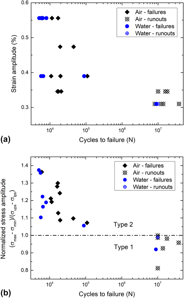
Strain-life data for all successful tests are shown in Fig. 12(a). As the strain amplitude decreases, an abrupt transition from failures to runouts can be seen in the data, indicating the existence of a fatigue threshold. However, we notice a nonmonotonic ε-N behavior in Fig. 12(a): some of the 0.44% strain (50 µm displacement amplitude) specimens exhibit lower life times than their 0.52% (55 µm) counterparts. A likely explanation for this response follows.
Fatigue data for tension–tension fatigue of dog bone-shaped specimens. (a) Strain–life data; (b) Life data expressed in terms of normalized stress amplitude (SA). The horizontal line at 1.0 represents the boundary between Type 1 and 2 loading, and correlates well with the fatigue threshold—when SA < 1, all specimens except for one are runouts. All specimens with SA > 1 are failures.

Within the tested specimens there were two types of variations: (i) variation in the initial slope of the load–displacement curve, i.e., during loading of austenite prior to commencement of the phase transformation; and (ii) variation in the plateau stresses. The consequence of these two variations is that the strain amplitude (computed from displacement amplitude without accounting for these variations) does not fully characterize fatigue loading and whether a given specimen was loaded in Type 1 or Type 2. Cyclic stresses rather than strains will provide greater insight into this set of fatigue life data.
The effective modulus varies strongly with temperature [Reference Robertson, Pelton and Ritchie2] and is a function of the difference between the loading temperature and the A f. In a commercial Nitinol batch, there is usually a 5°–10° variation in the A f, which translates to a variation in effective modulus. Another source of modulus variation arises from the stress-induced R-phase transformation; the propensity for, and the extent of this transformation, depend on the proximity of the test temperature to the A f temperature [Reference Duerig and Bhattacharya32]. For fatigue testing, a modulus variation implies that a given strain or displacement amplitude can give rise to different stress amplitudes.
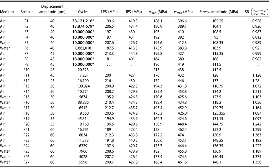
As previously noted in Section “Displacement-controlled quasi-static tensile loading, cyclic loading and fatigue testing”, Type 1 loading requires the stress range during cyclic loading (Δσ = σmax − σmin) to be lower than the stress hysteresis (difference between the upper and LPSs). Likewise, when the stress range exceeds this stress hysteresis, Type 2 cyclic loading results. The same can be expressed in terms of a normalized stress amplitude, SA = (σmax − σmin)/(σups – σlps). Type 1 loading corresponds to SA < 1, and Type 2 loading occurs when SA > 1. SA was computed for all the specimens by computing (i) the nominal stress maxima and minima from the load and the cross-sectional area at the narrowest portion of the cross section, and (ii) the upper and LPSs. In two specimens, the data from the initial loading curve were not recorded and so the stress ratio could not be computed. In Table I, the displacement amplitude, maximum and minimum strain and stress, strain and stress amplitudes, the upper and LPSs, and the stress ratio SA for the tested specimens are reported, and a fatigue life chart plotting the stress ratio against cycles to failure is shown in Fig. 12(b). All Type 2 specimens (SA >1) failed. Type 1 specimens were runouts to at least 10 million cycles with one exception: A specimen tested in water with SA = 0.92 failed after 8.8 million cycles.
Fatigue life data from specimens cycled under displacement-controlled loading at 40 Hz. Cycle numbers with an asterisk indicate runouts past 10 million cycles.
Discussion
We have outlined a new experimental approach for investigating Nitinol fatigue in a mixed-phase state, which is of relevance to medical devices. The main difference from prior work is the inclusion of all four of the following features in our experiments: (i) a marginally center-tapered dog-bone tensile specimen geometry that gives rise to a single martensitic band within the austenite gage section, (ii) the use of a high-speed camera for DIC and for surface imaging during displacement controlled tensile cyclic loading, (iii) nonzero mean strain during cycling, and (iv) a preloading procedure that simulates the crimp-and-deploy procedure in a flat dog-bone tensile specimen rather than on a complex-shaped stent subcomponent. These features enabled a clearer understanding of strain distribution in the coexisting phases and in the transition zone between them in two very different loading profiles (Type 1 and Type 2) and the influence (or lack thereof) of the imposed frequency on cyclic response.
This combination of cyclic loading, DIC, surface imaging, and fatigue testing addressed the questions set out in section “Introduction”, and have led to the following insights:
(i) Strain localization resulting from the SIMT leads to varying mean strain and strain amplitudes across the specimen.
(ii) At high displacement amplitudes, high cyclic strains accommodated by cyclic SIMT are localized to small transition zones sandwiched between the martensite band and the austenite regions flanking it.
(iii) Fatigue crack initiation occurs at near-surface inclusions situated within one of the two austenite co-existing martensite transition zones.
(iv) Loading involving cyclic SIMT resulted in fatigue failures, whereas loading without SIMT, where deformation is nominally elastic (with a minor anelastic component) and perhaps some austenite to R-phase transformation, led to runouts up to 107 cycles in all but one specimen. The fatigue threshold defined as the strain amplitude limit that separates the two regimes is determined by the forward and reverse transformation stresses or plateau stresses and the effective elastic modulus; this can be estimated from the tensile loading curve and can also be expressed nondimensionally as a normalized stress amplitude.
(v) Cyclic mechanical response is frequency dependent only in the presence of cyclic SIMT. Use of water as a test medium does not suppress this frequency dependence. Higher strain rates hinder, but do not suppress SIMT completely.
Crack initiation during displacement-controlled cyclic loading within the transition zone and subsequent growth perpendicular to the principal stress is similar to that reported by Zheng et al. [Reference Zheng, He and Moumni10]. In that stress-controlled fatigue study, the authors noted crack initiation in what they refer to as “active zones” that underwent cyclic SIMT, although it wasn’t clear why a specific active zone was preferred to others. The single martensitic band in the present study illustrates the link between SIMT and low cycle fatigue failures with greater clarity. It is worth noting that crack initiation does not occur within the martensite at the narrowest portion of the gage section where the nominal stress is the highest. This implies that the local stresses at the austenite–martensite interface are higher as previously noted in Ref. Reference Sedmák, Pilch, Heller, Kopeček, Wright, Sedlák, Frostand and Šittner33 and offset the marginal areal reduction in the central gage section of the marginally center-tapered specimen. A higher resistance to crack initiation in the martensite could also explain this observation. In any event, SIMT plays a dominant role in the damage accumulation process.
In section “Introduction,” based on previous superelastic cycling data [Reference Melton and Mercier3, Reference Kim6], and rotary beam bending fatigue data [Reference Eggeler, Hornbogen, Yawny, Heckmann and Wagner7, Reference Wagner, Sawaguchi, Kausträter, Höffken and Eggeler8, Reference Reinoehl, Bradley, Bouthot and Proft17, Reference Sheriff, Pelton and Pruitt18, Reference Morgan, Wick, DiCello and Graham19], both of which showed abrupt transitions in ε-N curves at the point of activation of SIMT, we conjectured that similar patterns could hold true in mixed-phase loading. Fatigue life data in the present study confirm this hypothesis: they show an abrupt transition from low-cycle failures to high-cycle runouts approximately when the strain amplitudes fall from Type 2 to Type 1 levels. Melton and Mercier [Reference Melton and Mercier3] have shown that repeated superelastic cycling between 0 and 6% strain led to fatigue failures in the low-cycle (103–105) regime in annealed Nitinol, and similar observations were recently made in commercial cold-worked Nitinol as well [Reference Zheng, He and Moumni10]. In the present study, DIC analysis showed that local strain amplitudes in the transforming regions in Type 2 loading approach this level even though global averages are far below. Supporting this assertion are surface observations by high-speed photography that showed crack initiation occurring in/near the transition zone. This leads to the conclusion that cyclic SIMT in a small portion of the specimen is sufficient to cause low-cycle fatigue failures.
The present uniaxial fatigue data indicate that the fatigue threshold for tension–tension is the strain amplitude that separates Type 1 and Type 2 loading, which can be roughly estimated from quasi-static uniaxial tensile data. In section “Fatigue life data,” Type 1 and Type 2 loading were distinguished by the value of the normalized stress ratio (SA): For SA > 1, low-cycle fatigue failures occur and for SA < 1, high-cycle life up to at least 107 cycles is likely. The threshold is at SA = 1; or stated alternately, when the stress range during cyclic deformation is equal to the stress hysteresis. Thus, in terms of stress amplitude, the fatigue threshold Δσl is
 $$\Delta {\sigma _{\rm{l}}} = {1 \over 2}\left( {{\sigma _{{\rm{ups}}}} - {\sigma _{{\rm{lps}}}}} \right)\quad ,$$
where σups and σlps are the upper and LPSs, respectively. We obtain the strain-based fatigue threshold Δεl by dividing the above quantity by the effective elastic modulus as follows:
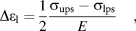 $$\Delta {\varepsilon _{\rm{l}}} = {1 \over 2}{{{\sigma _{{\rm{ups}}}} - {\sigma _{{\rm{lps}}}}} \over E}\quad ,$$
where the effective modulus E is given by
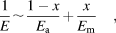 $${1 \over E}\sim{{1 - x} \over {{E_{\rm{a}}}}} + {x \over {{E_{\rm{m}}}}}\quad ,$$
where E a and E m are the elastic moduli of austenite and martensite, respectively, and x is the martensite volume fraction. Thus, the fatigue threshold can be estimated from parameters calculated from the tensile loading curve. Alternatively, a normalized stress amplitude below 1 can be used as a stress-based criterion for survival into the high-cycle fatigue regime (>1 million).
If the fatigue threshold is only dependent on tensile behavior, the role of inclusions in fatigue needs clarification, given that inclusions were found at crack initiation sites. It is known that inclusions are crack initiators [Reference Robertson, Pelton and Ritchie2]. Yet this does not necessarily imply that the fatigue threshold is the stress intensity threshold (ΔK th) required for crack initiation from inclusions as in other elastic–plastic materials. Cyclic SIMT plays an important role. Furthermore, the likelihood of the SIMT threshold (SA = 1) and the crack initiation threshold stress intensity (ΔK th) at inclusions being identical is low in the present study. It is possible that for inclusions of the size encountered in the present study and for smaller ones, they are merely proximate causes of fatigue crack initiation, while the SIMT serves as the higher-level ultimate cause. Conversely, if the inclusions or defect sizes grew larger beyond a certain point, the crack initiation threshold from inclusions may become lower than the SIMT threshold. Thus, depending on the inclusion size, the SIMT or the inclusions could determine the fatigue crack initiation threshold.
The above line of reasoning leads to another conclusion: In tension, the fatigue threshold is capped by the SIMT threshold, and therefore cannot be increased indefinitely by reducing the inclusion size. Zhang and James [Reference James, Zhang, Planes, Manosa and Saxena34] have postulated that elastic incompatibility at the austenite–martensite interfaces during SIMT is the primary cause of hysteresis during SIMT. The second eigen value of the distortion matrix must be equal to 1 for perfect compatibility, which is not satisfied by most shape memory alloys including Nitinol. Prior work indicates that dislocations accumulate due to repeated SIMT [Reference Melton and Mercier3, Reference Pelton15]. Elastic incompatibility may be responsible for dislocation accumulation which may eventually lead to fatigue crack initiation and failure. Chluba et al. [Reference Chluba, Ge, Lima de Miranda, Strobel, Kienle, Quandt and Wuttig35] have demonstrated in a multicomponent shape memory alloy with very low hysteresis (near-perfect compatibility) that it can run out to 107 cycles without failure while undergoing the full SIMT. This shows the converse is true: with perfect or near perfect compatibility, SIMT can occur indefinitely without leading to failure. In NiTi alloys, since perfect compatibility does not exist at the interface, the fatigue threshold in tension is unlikely to increase beyond the phase transformation threshold.
The estimation of the fatigue threshold based on tensile data is a powerful tool for materials selection and design. Whereas this was relatively straightforward in tension, such is not the case in bending as discussed below.
In stent subcomponent (diamond-shaped struts) fatigue testing with predominantly bending loads and a mixed-phase starting condition, ε-N data can often be bimodal [Reference Pelton, Schroeder, Mitchell, Gong, Barney and Robertson24, Reference Pelton, Gong, Duerig and Shrivastava30] in much the same way as in our uniaxial tests. In other cases, the ε-N curve shows a “knee,” where the usual gap between the low cycle failures and high cycle runouts (105–107 cycles) is filled with failures but those that occur at a near-constant strain amplitude [Reference Robertson, Launey, Shelley, Ong, Vien, Senthilnathan, Saffari, Schlegel and Pelton25]. In either case, there is a fatigue threshold or strength expressed as the spatial maximum of strain amplitude on the tensile side of the bending members. Although this bears resemblance to the case of uniaxial tension where the fatigue threshold is nearly equal to the SIMT threshold, data are insufficient to conclude that the two are identical. The stress and strain gradients differ substantially in bending from those observed in tension. Consequently, the strain localization phenomenon observed in uniaxial tension might not occur to the same degree in bending because of naturally present mechanical constraints. Thus, the sharp dichotomy between activating and not activating SIMT may not exist at the macroscopic scale. Further work is necessary to understand how this difference manifests in fatigue damage accumulation.
Unlike in dog-bone specimens under tension, the strain amplitude estimation in stent subcomponents requires finite element modeling that employs a complex material model. Also, the compression behavior (UPS, transformation strain) strongly influences the bending response. While the FE models usually capture tension-compression asymmetry, pertinent compression data are often unavailable, and are therefore assumed. The variations in effective elastic moduli due to R-phase and strain localization are not captured in usual finite element models. Thus, the spatial maximum of strain amplitude computed from finite element analysis is approximate. Though this approach is adequate for and successful in assessing performance of Nitinol components, additional data such as local strain measurements or more sophisticated finite element models are necessary for assessing the link between SIMT and fatigue damage.
Furthermore, the use of the spatial maximum of strain amplitude as the primary metric for characterizing fatigue has limitations. The strain amplitude is a sum of elastic, transformation, and plastic strain. These different physical mechanisms do not contribute equally to fatigue damage, and, therefore, must be weighted appropriately. For example, in tension, we find that the contribution of the transformation strain is dominant. In bending, the spatial maximum of strain does not indicate the size of the stressed volume, and the volume that may be undergoing SIMT, both of which are often microscopic in bending and will depend on the geometry of the implant. The probability of finding inclusions in the stressed volume is likely important [Reference Bonsignore36]. All of these must be considered in characterization and prediction of fatigue in Nitinol structures. Given the importance of fatigue in Nitinol implants, the influence of the phase transformation on fatigue life and threshold in bending warrants further inquiry, as it may lead to better predictive models of fatigue damage.
If the SIMT threshold can be used to determine the fatigue strength in bending, then it should be possible to calculate it using finite element analysis by simulating stress fields around inclusions. Resource-intensive fatigue testing during material selection and device design could be greatly reduced and employed at fewer stages of the design process. This would additionally lead to fatigue improvement strategies in addition to inclusion size reduction, such as processing methods that alter the SIMT characteristics. For instance, in the simple scenario of the SIMT threshold being equal to the fatigue strength, the displacement-controlled fatigue strength could be increased by (i) decreasing the effective modulus as proposed by Duerig et al. [Reference Shamimi, Amin-Ahmadi, Stebner and Duerig37] and (ii) increasing the difference between the upper and lower plateaus stresses. Our data were collected only to 107 cycles and for tension–tension fatigue. Further work is needed for obtaining data out to 6 × 10⁸ cycles and in bending to realize this possibility. Nevertheless, the present data and observations taken together with prior experimental observations [Reference Pelton, Schroeder, Mitchell, Gong, Barney and Robertson24, Reference Robertson, Launey, Shelley, Ong, Vien, Senthilnathan, Saffari, Schlegel and Pelton25, Reference Runciman, Xu, Pelton and Ritchie38] are strong motivators for future work to extend the findings to bending and into very high cycle fatigue.
Prior research has confirmed that adiabatic heating during phase transformation leads to rate dependence in monotonic mechanical response [Reference Shaw and Kyriakides26] as well as fatigue life [Reference Wagner, Sawaguchi, Kausträter, Höffken and Eggeler8], if no attempts are made to maintain constant temperature. While Wagner et al. [Reference Wagner, Sawaguchi, Kausträter, Höffken and Eggeler8] showed that rate dependence in fatigue life can be suppressed by using temperature-controlled silicon oil as a test medium, it is not clear if this is true of water and water-based media like saline commonly used for Nitinol fatigue testing. In fact, the earlier work by Shaw and Kyriakides [Reference Shaw and Kyriakides26] showed that rate dependence in monotonic mechanical response persists in water. Our present data confirm that this is true of cyclic loading as well: mechanical response in Type 2 loading is loading frequency-dependent and higher rates of loading result in smaller volumes undergoing phase transformation. Consistent with this, the simpler case of Type 1 loading is not loading frequency dependent. This also implies that the fatigue threshold in tension, which we have defined as the upper limit of Type 1 loading, is not dependent on loading frequency. To fully assess the impact of loading frequency on crack growth rates and fatigue life, additional work is necessary.
In the context of fatigue of medical device components, additional factors must be taken into consideration. Implanted Nitinol components (i) have smaller cross-sectional areas than the dog bones used in the present study, (ii) are subject to cyclic-bending dominated loading mode where stress and strain gradients are present, and (iii) are loaded in vitro or in vivo in a water-based solution at constant temperature. Consequently, the volume undergoing phase transformation is much smaller in comparison to the dog bones under tension–tension loading used in the present study. Furthermore, adiabatic effects that give rise to loading frequency dependence are minimized. Thus, the loading frequency dependence of fatigue life is not expected to be significant in medical device components. Robertson et al. [Reference Robertson and Ritchie14] have provided a strong rationale for the practice of accelerated fatigue testing of Nitinol components based on crack growth rate measurements in compact tension specimens.
Summary and conclusions
We describe a new experimental approach for investigating fatigue in Nitinol within the context of medical devices that undergo cyclic loading in the mixed-phase state. From it, we have gained new and important insights into Nitinol fatigue that are of particular relevance to medical device engineering. Tension–tension cyclic loading experiments were performed at three different strain rates on slightly center-tapered dog-bone specimens cut from superelastic Nitinol sheets. All specimens were subjected to a preloading procedure that simulates crimping and deployment of a Nitinol stent or transcatheter heart valve, where the gage section was loaded to 6% average strain followed by partial unloading to 3% average strain. Strain localization and phase transformation during cyclic loading were investigated using DIC, and crack initiation and growth were observed and recorded by means of a high-speed camera. Strain–life fatigue data were obtained under displacement-controlled conditions for a cyclic frequency of 40 Hz. A few specimens were tested in water to understand the impact of testing medium on the fatigue threshold. The following conclusions are drawn from this study.
(1) Because of the localized nature of the stress-induced martensitic phase transformation (SIMT), the mean and alternating strains during tensile cyclic loading vary substantially across the specimen gage section, especially when the threshold for SIMT is exceeded.
(2) Above the SIMT threshold (Type 2), the transformation is localized to small regions bordering the austenite–martensite interface (transition zones) where local strain amplitudes approach 2–4x the average.
(3) Crack initiation occurs in Type 2 loading within the region undergoing forward and reverse SIMT, at/near the austenite–martensite transition region and typically at a near-surface inclusion. Crack propagation occurs rapidly along the plane of maximum principal stress and failure occurs within 5% of the total fatigue life of the specimen after crack initiation.
(4) In uniaxial tension, fatigue failures in the low-cycle fatigue regime are caused by macroscopic cyclic SIMT; keeping the strain amplitude low enough to avoid SIMT extends the fatigue life into the high-cycle regime beyond 107 cycles. Thus, for the present specimens, the fatigue threshold is simply half the stress or the strain amplitude required to initiate SIMT.
(5) In uniaxial tension, we hypothesize that the displacement-controlled fatigue threshold for mixed-phase cyclic loading can be estimated from the tensile superelastic curve. Further work in tension, and in Nitinol, with smaller inclusions is needed to confirm the generality of this finding in tension. It is also necessary to explore the utility/validity of this principle in bending.
(6) Cyclic response in tension is loading frequency dependent only above the fatigue threshold, where the stress-induced phase transformation mechanism operates. The low-cycle fatigue life in tension could be loading frequency and medium dependent. However, the fatigue threshold itself, which is of greater engineering relevance in medical devices, is unlikely to be loading frequency dependent in the 0.004–40 Hz range. Given the smaller volumes undergoing SIMT in Nitinol components under cyclic bending, loading frequency dependence is not expected to be significant.
Acknowledgments
We thank Herwig Mayer and Michael Fitzka at the University of Natural Resources and Life Sciences, Vienna, Austria, for providing the fatigue specimen design for use in this study. We thank James Hallquist for conducting several of the fatigue life tests. We also thank Mallika Kamarajugadda, Richard Francis, Markus Reiterer, Curtis Goreham-Voss, Scott Terry, and Shivram Sridhar at Medtronic plc for their many helpful discussions and comments that significantly improved this manuscript. Sharvan Kumar and Zhiwei Ma acknowledge Medtronic for the research grant to Brown University that enabled this collaborative work.