Introduction
Many important materials are defined by a single underlying interaction or force, which allows modeling using analytical expressions having relatively few parameters. Examples include ferromagnets, where the magnetism is described by the exchange interactions between spins[Reference Kittel1] and elastomers, where the resistance to deformation is due to polymer chain entropy.[Reference Flory2] In contrast, the properties of complex materials are determined by multiple competing forces, the interplay of which lead to a rich diversity of physical properties and performance characteristics. Complex materials, such as complex fluids,[Reference Stickel and Powell3] metal alloys,[Reference DeCost, Francis and Holm4] and catalysts,[Reference Saravanan, Kitchin, von Lilienfeld and Keith5] are ubiquitous, but predicting their properties remains a significant challenge.
Machine learning (ML) is a diverse collection of powerful techniques utilized to identify relationships in data, allowing for modeling and optimization of complex systems. With rapidly growing datasets available, ML has become a robust methodology applied across many materials disciplines and has been increasingly incorporated in conjunction with the Materials Genome Initiative.[Reference Ramprasad, Batra, Pilania, Mannodi-Kanakkithodi and Kim6–Reference McDowell and Kalidindi8] However, the traditional methods of ML are based only on statistical inference, requiring large datasets to develop predictive models that connect composition and processing with properties. While some disciplines within materials science, such as metallurgy[Reference Qin, Lin, Wei, Zhu, Yuan, Takeuchi and Jin9] or heterogeneous catalysis,[Reference Gani and Kulik10] have developed methods for high-throughput experimentation to produce sufficiently large datasets, most disciplines still use traditional methods of materials preparation and analysis, precluding the use of ML methods designed for Big Data.[Reference Ramakrishna, Zhang, Lu, Qian, Low, Yune, Tan, Bressan, Sanvito and Kalidindi11,Reference McBride, Persson, Reichmanis, Grover, McBride, Persson, Reichmanis and Grover12]
While, in the case of systems described by an exactly known relation, a physical law is better utilized, in complex systems, a single physical relation may not exist, but several relations could underlie the system. These constituent physical relations can be utilized in conjunction with ML to learn the interplay of interactions within these complex systems, and with the increasing use of data-driven approaches, science has utilized traditional ML to predict molecular solubility,[Reference Kuhne, Ebert and Schuurmann13–Reference Sanchez-Lengeling, Roch, Perea, Langner, Brabec and Aspuru-Guzik15] discover new thermodynamically stable materials,[Reference Meredig, Agrawal, Kirklin, Saal, Doak, Thompson, Zhang, Choudhary and Wolverton16] and determine highly accurate interatomic potentials.[Reference Hansen, Biegler, Ramakrishnan, Pronobis, von Lilienfeld, Müller and Tkatchenko17] While a simple, single physical law could be learned through statistical inference techniques with a small dataset of, say, 10 datapoints, systems defined through several complex relations can require the use Big Data in the range of thousands or more datapoints to accurately model. In general, the amount of data needed depends on the ratio of datapoints to the number of features. If a small number of features can effectively model the data, then fewer datapoints are needed. However, as the complexity of the system increases, the higher number of features needed to model the system would require a higher number of datapoints to effectively model.
It is still possible to use the tools of ML on small datasets, but this requires the development of hybrid algorithms that embed domain knowledge in order to develop predictive models that relate system variables to system responses, thus narrowing the search space that data-driven models must explore. In the context of materials science, domain knowledge can take a number of forms, and here four different types are surveyed: (i) physicochemical properties, (ii) similarity, (iii) system properties, and (iv) physical laws and empirical equations. This review will discuss these types of domain knowledge as well as specific examples of how they are implemented in ML algorithms. Finally, a prospectus on how these approaches can be used in the important problem of transfer learning to bridge across multiple systems will be presented.
Response surfaces and machine learning
The general task here is to understand how changes in experimental or system variables change the properties of the system. For complex systems, high costs and time demand limit data collection to small datasets,[Reference Liu, Zhao, Ju and Shi18] with examples including adhesives, agrochemicals, pigments, paints, coatings, lubricating oils, paper, and pharmaceuticals, all of which have limitations in the amount of data that can be acquired under realistic resource assumptions.[Reference Rowe and Colbourn19,Reference Tanco, Viles, Ilzarbe and Alvarez20] Design of experiment (DOE) approaches are a common tool for estimating the response surface of such systems based on the incomplete exploration of the variable space. In the DOE approach, system features are systematically varied, so that outputs can be mapped as a continuous response surface. These observations allow the discovery of correlations between features and produce a function that can be subsequently optimized.[Reference Montgomery21] A common method utilized with the DOE is a full-factorial design. In this approach, each of the k-factors (features) are tested at n levels. For example, if n = 2, the design will measure the value of the response as maximum and minimum values of each feature against the maximum/minimum values of every other feature resulting in 2k simulations being performed. The benefits of DOE allow for correlations between features to be discovered and a response surface to be mapped, but disadvantages of the approach include limits to the non-linearity of the surface being mapped, exponential growth of the system with increasing feature size, and large uncertainty of the surface response mapping in areas that are untested, as illustrated schematically in Fig. 1. Establishing a technique to embed domain knowledge would allow for the response to be better predicted between test points by training the algorithm to understand the relationships between system variables and how they determine system responses.
Illustration of two possible response surfaces that fit the four points of a training set shown as green circles. The red concave surface represents a simple model from the DOE where the response surface was modeled with a second-order polynomial. This approach fails to capture complex underlying interactions, which could take place throughout the domain space, as shown in blue.

ML techniques are applied across systems as diverse as clinical medicine, facial recognition, self-driving automobiles, and scientific fields such as cheminformatics and bioinformatics. The development of such diverse uses of ML has been predicated on using Big Data (datasets routinely including millions of points) enabled by acquisition over large populations, such as high-throughput measurements.[Reference Jordan and Mitchell22] In recent advances, ML techniques utilizing image recognition for detecting melanoma have outperformed medical experts in diagnosing.[Reference Haenssle, Fink, Schneiderbauer, Toberer, Buhl, Blum, Kalloo, Ben Hadj Hassen, Thomas, Enk, Uhlmann and Holger Haenssle23] Where sufficient data are present, ML algorithms have the capability of learning relationships between inputs and outputs; however, unlike human learning, traditional ML techniques relying on raw features perform poorly at determining relationships utilizing small datasets.[Reference Griffiths, Baraff and Tenenbaum24] Foundational research has previously been applied toward developing a general unified theory of learning in conjunction with ML and emphasized the need for the development of multi-strategy techniques for learning on various types of data, but these have not been widely implemented for use in small datasets.[Reference Michalski25]
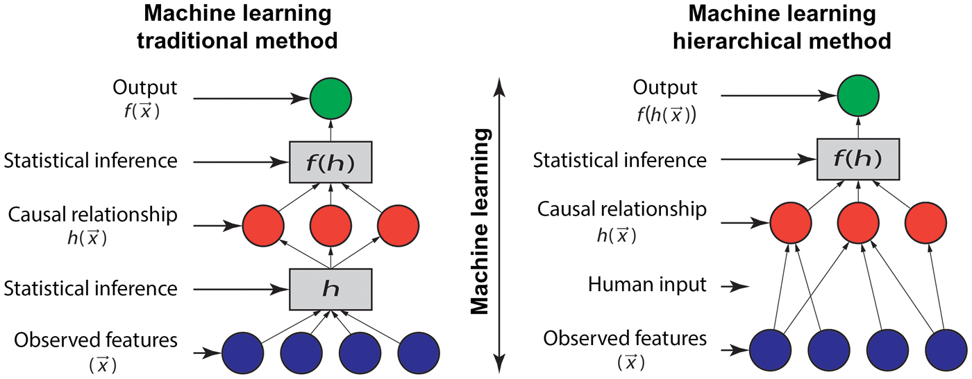
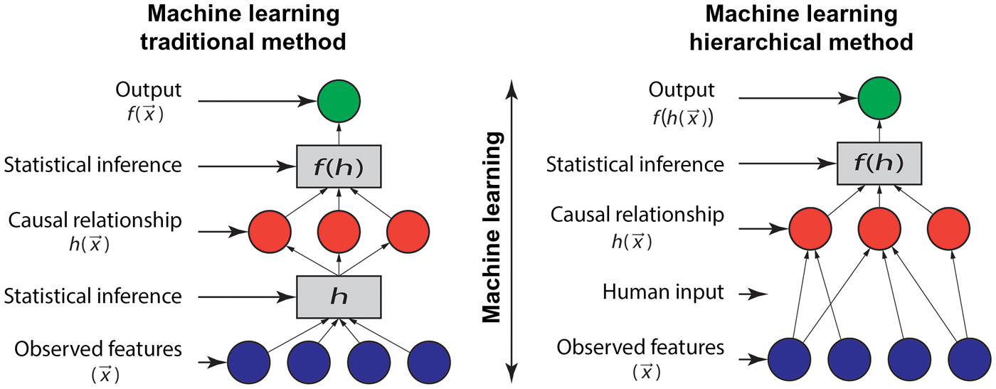
Fields such as cognitive neuroscience, which began incorporating early ML techniques to model human learning as early as the 1960s,[Reference Carbonell, Michalski, Mitchell, Michalski, Carbonell and Mitchell26] have attempted to better predict the relationship between inputs and outputs by explicitly including causal relations, allowing algorithms to learn on small data.[Reference Griffiths, Baraff and Tenenbaum24,Reference Tenenbaum, Griffiths and Kemp27] For example, recent research has demonstrated human-level performance for “one-shot” recognition of handwritten characters on sparse datasets. Causal knowledge was included through parsing characters into the training set by each “pen stroke,” allowing the model to take into account how the characters were drawn to identify each character.[Reference Lake, Salakhutdinov and Tenenbaum28] The causal relationships create a hierarchical model where domain knowledge can be explicitly included or learned to be included in future models. This approach relates the inputs of a system to a middle layer as opposed to traditional ML where inputs are related through statistical inference in hidden layers (which may or may not be explicitly included in the algorithm) as shown in Fig. 2.
The traditional model directly predicts the outputs from the inputs with learned causal relationships. The hierarchical model allows for the incorporation of domain knowledge through human input before predicting outputs.
However, incorporating domain knowledge into ML algorithms needs to be performed in a way which does not block the discovery of unexpected solutions. An heuristic example of this is the statement that “trucks can't drive over water,” but this domain knowledge ignores the possibility of the water freezing in winter.[Reference Frawley and Piatetsky-Shapior29] Translating real-world phenomena, such as temperature variations, into ML problems requires expert knowledge so as to not eliminate possibilities that could be discovered using data-driven approaches.[Reference Sacha, Sedlmair, Zhang, Lee, Peltonen, Weiskopf, North and Keim30]
Research areas in which small datasets are commonly generated face two challenges in adopting ML techniques. The first, as discussed, is the challenge in making accurate predictions using methods based strictly on statistical inference. The second is that experimental design in a laboratory setting tends to be sequential and driven by intuition, and experimental parameters naturally tend toward values that lead to maximizing (or minimizing) an objective function. This artificially limits the dataset to a narrow section of the input variable space and does not adequately train the algorithm on the range of system responses that can be generated, limiting as Jain et al. described, the “completeness” of the dataset.[Reference Jain, Hautier, Ping Ong and Persson31] These point to the importance of embedding domain knowledge in ML algorithms to use causal relationships as hypotheses. While incorporating causal relationships to human learning is difficult to formalize,[Reference Tenenbaum, Griffiths and Kemp27] extensive and formalized knowledge of them are the basis of scientific model building. Through an expert's appropriate incorporation of domain knowledge, a hypothesis-space of the domain knowledge can be created on which to train.[Reference Wu, Suetens, Oosterlinck, Piatetsky-Shapiro and Frawley32] From this perspective, ML can be an effective tool for the unbiased analysis of complex material systems with small datasets.
Here, we discuss methods of embedding physical knowledge into ML algorithms. Instead of experimentally defined descriptors being directly used as the sole inputs for ML, selected inputs also include physical factors modeling the system. This embedded knowledge can take the form of correlative relations, such as identifying similarity metrics, empirical relations in the form of physical equations, or embedding exact relations such as invariance properties. It will be shown that by embedding ML algorithms with these techniques, small data can be utilized to effectively model a complex material system.
Methods
ML encompasses many varying algorithms. To provide an understanding to some of the basic algorithms being surveyed through this review, an overview of these methods will be provided.
Cross-validation
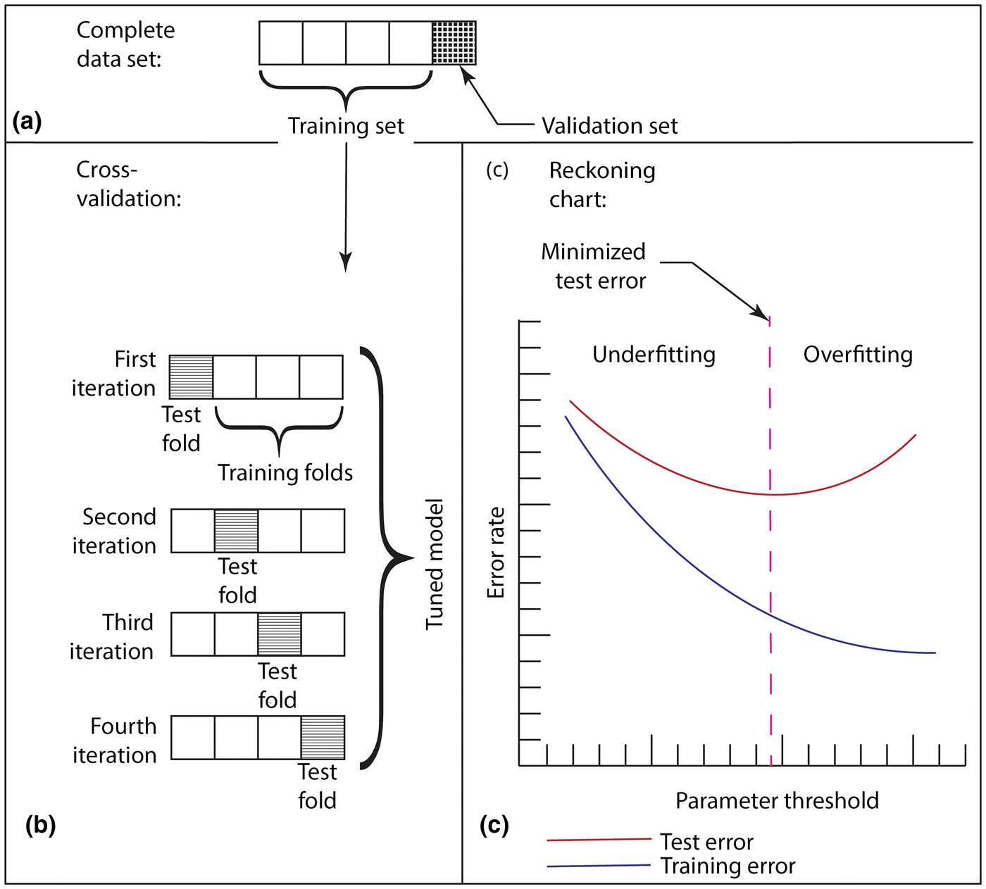
ML centers on the development of algorithms that improve in the performance of a given task with experience.[Reference Jordan and Mitchell22] Experience, in terms of scientific research, is synonymous with acquiring experimental or computational data. A collection of inputs, sometimes termed features or descriptors, is utilized to improve the prediction accuracy through ML, and to establish a relation between inputs and outputs, a direct relation in the form of a regression can be predicted. There are numerous variations of regression methods used in ML, and each attempt to achieve the same goal: establishing an accurate model of the response surface for a complex system on test data. To establish a best-fit to unseen (test) data, regression models have their parameters learned on training data through a process called cross-validation as shown in Fig. 3. However, validity of the model is not assessed until it is applied to new data, and this also requires that it has an appropriate level of complexity. As illustrated in Fig. 3, while training error decreases monotonically with model complexity, the accuracy of predictions on test data reaches a minimum at intermediate complexity – overly simple models do not predict training or test data, but overly complex models are only valid on training data. Data-driven approaches require both the optimization of model parameters and model complexity. These basic criteria also hold true when domain knowledge is incorporated.
(a) The first step of cross-validation is to partition the complete dataset into both a training set in which parameters will be optimized against and a validation set in which error between experimental data and predicted regression is compared. (b) This shows an example of a k-fold cross-validation where the training set is split into training and test folds. Each subset of the sample is treated as a test fold through one of the iterations and an optimum parameter is chosen which minimizes the test error. (c) The parameter chosen falls in between a regime of underfitting and overfitting, where underfitting only exhibits small correlation to the dataset and overfitting minimizes the training error but begins to show an increase in test error. This optimized parameter would provide the most accurate fit to the validation set.

Linear regression
Ordinary linear regression is a well-known statistical technique that fits a linear model to a dataset. A common approach to optimizing the fit of data to a linear regression is through minimizing the sum of squared residuals, or the sum of squared distance between a datapoint and the best-fit line. These linear least-squares regressions have a trivial solution for the β-coefficients where the equation for a line is:

and where the β-coefficients corresponding to a minimized sum of squared residuals are:

The trivial solution to β is:

Linear regressions can also be regularized and include additional parameters which are optimized through cross-validation. The least absolute shrinkage and selection operator (Lasso) was originally developed in 1996 by Tibshiranit.[Reference Tibshirani33] Similar to ordinary linear regression, Lasso finds the minimized sum of squared residuals with an additional penalty term penalizing the L1 norm, or sum of the absolute value of β-coefficients:

The lambda parameter is learned through cross-validation and the value assigned to predicting the lowest test error is selected. At this point, non-important features have their β-coefficients reduced to zero and are eliminated from the calculated equation. If the penalty term in Lasso is set to zero, the regression is reduced to an ordinary linear regression where all β-coefficients contribute to the final calculated equation.
Neural networks
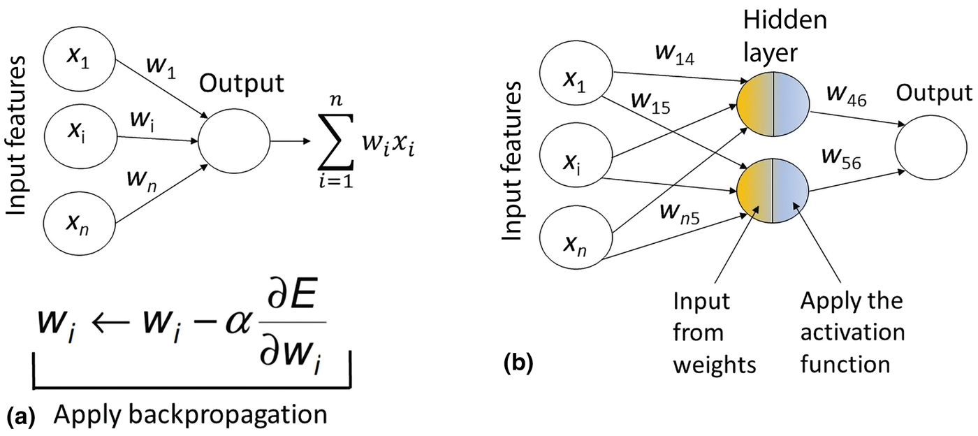
Neural networks, a robust form of ML sometimes referred to as deep learning networks, are algorithms used for pattern recognition and regression.[Reference Mitchell34] These networks are composed of multiple layers of neurons: an input layer, hidden layer(s), and an output layer. The output of each neuron is passed to those in the next layer with an associated weight. The hidden layers and output layer also contain associated activation functions that are tuned while learning relationships between the input and the output using the training data. Activation functions can either be linear or nonlinear, with a common nonlinear choice being a sigmoid function. After the initial input is forward-processed through the network, the output is compared to the target (correct) output value, and the associated error is calculated between the target value and the output value from the neural network. A methodology known as backpropagation is then applied to minimize the error, updating the weights between neurons. Through these updates, the error is minimized to an optimal value determining the best-fit curve to the data. By increasing the number of neurons and activation–function complexity in the network, the complexity of the regression increases. Figure 4 provides a schematic of a two-layer network (perceptron) and a representation of a higher complexity network.
(a) A simple neural network is known as a perceptron. This perceptron is made up of an input layer connected to an output layer through a linear activation function. A method of backpropagation, stochastic gradient descent, is shown where α is the learning rate hyperparameter, which controls how fast the weights are updated with the associated error through every iteration. The perceptron shown is the same as performing ordinary linear regression. (b) This shows a more complex network with an included hidden layer. This hidden layer takes inputs and feeds them into an activation function before predicting an output.

Random forest
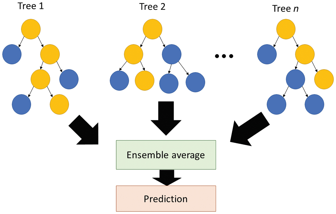
Random forests are made up of an ensemble of decision trees, and for regression purposes, the output of all these trees has an average taken to produce a singular best-fit regression for the entire collection of trees. Each tree is split utilizing bootstrapping, a technique of resampling the dataset many times, with replacement, to test on each tree.[Reference Mooney and Duval35] Each bootstrap tree is split on the collection of all features utilizing a random subset of the features with replacement for every split. The special case where the random subset of features is equal to the total number of features is known as bagging.[Reference Svetnik, Liaw, Tong, Culberson, Sheridan and Feuston36] A recursive binary process of splitting, where the feature to split on is determined through splitting on the feature which maximizes the reduction in some metric such as the sum of squared errors, is continued at each node either until reaching a user-specified end or until complete separation has occurred.[Reference Xu, Watanachaturaporn, Varshney and Arora37] To control overfitting, the maximum depth of the trees along with post-processing methods, such as pruning, can be utilized. The number of trees can also be controlled and is typically enough when the prediction made by the forest is approximately equal to the prediction of a subset of the forest.[Reference Liaw and Wiener38] Regression trees work through recursive partitioning and therefore an exact function cannot be fit to the model. The predictions to the regression are determined the ensemble averaging of each tree in a random forest as shown in Fig. 5.
A collection of n decision trees are created according to bootstrap and bagging techniques. The yellow path in each tree corresponds to the same predicted output. The ensemble average of these collected outputs corresponds to the final prediction as produced from a random forest regression.

Bayesian probability and Gaussian processes
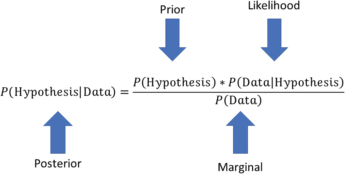
A Gaussian process (GP) is based on the concept of including a Bayesian probabilistic approach. Bayesian probability determines the posterior probability of an event based on the probabilities of the factors constituting the event – prior probabilities and likelihood of these occurring as shown in Fig. 6.
Bayes' theorem states that the posterior probability of a hypothesis occurring given data can be calculated through the prior probability a hypothesis is true before collecting data, the likelihood that the data are collected given that the hypothesis is true, and the probability of collecting that data under all possible hypothesis.

The posterior probability is updated as part of the GP resulting in a regression with error terms represented across the range of the regression. While regression and neural networks are parametric approaches, in that the shape of the curve being fit to the data is defined, GP is a non-parametric approach, meaning that the best shape and the best fit curve are both learned through the regression process.[Reference Rasmussen, Bousquet, von Luxburg and Rätsch39] As a GP is a Bayesian approach, the entire process is defined by a mean and covariance function. While a Gaussian distribution is defined over a set of vectors, a GP is defined over a set of functions, that is:

where the optimized function, f, is distributed as a GP across the mean function μ and the covariance function ∑. Multiple covariance functions can be utilized, but the chosen function is a method of relating similarity. Covariance provides insights into how related two variables are through utilizing varying similarity metrics such as linear, squared exponential, periodic, or any combination of covariance functions, the covariance function learns similarity through mathematically representing assumptions about the function being learned.[Reference Rasmussen and Williams40] Utilizing the prior mean and covariance, an infinite number of possible functions is introduced to the feature space of the data. As data are introduced to the GP, the mean and covariance are updated at that point with the associated covariance function defining the error in areas without training data introduced, that is:

where a joint distribution is created between the function fitting the training data, f, and the function fitting the test data, f *, across the normal distribution across these functions. As the training function f is known, the conditional distribution, (f *|f), can be updated to solve for the new mean and error in the updated function.[Reference Rasmussen, Bousquet, von Luxburg and Rätsch39] Upon cross-validation, optimized parameters in the covariance function are selected defining the smoothness of the function and error between the training points.
Applications to material systems
Embedding physicochemical properties
In predictive models of molecular materials, quantum chemical (QC) parameters have been used to solve chemical Hamiltonians,[Reference Li, Collins, Tanha, Gordon and Yaron41] learn force field parameters,[Reference Li, Li, Pickard, Narayanan, Sen, Chan, Sankaranarayanan, Brooks and Roux42] represent crystal structures,[Reference Schütt, Glawe, Brockherde, Sanna, Müller and Gross43] and predict heats of formation.[Reference Hu, Wang, Wong and Chen44] Embedding physical knowledge with QC inputs improves predictive capabilities of ML algorithms and accelerates calculations,[Reference von Lilienfeld45] but these calculations add computationally intensive steps in ML analysis. However, more accurate descriptors can enable the use of simpler ML tools and smaller datasets.
The two important ML methodologies utilized in this paper were linear regression and artificial neural networks (ANNs), which both permit embedding of physicochemical properties to improve predictive capabilities. Linear regression is considered to be a simpler formalism, but its performance can rival that of the more complex ANNs when provided with a more accurate feature set. QC calculations,[Reference Gardas and Coutinho46,Reference Paduszyński and Domańska47] such as electronic charge distribution, dipoles, vibrational frequencies, and reactivity, have been used to increase the accuracy of predictions on ionic liquids. Mehrkesh and Karunanithi[Reference Mehrkesh and Karunanithi48] utilized QC-predicted descriptors of the symmetrical value, which describes packing density between anions and cations, as well as the distance between anions and cations, anion volume and surface area, and the dielectric energies of anion and cation liquids along with the temperature as a system condition. Each of these properties relates to important factors that impact the mobility of ions within a complex ionic liquid. Values of viscosity were aggregated from 20 sources for a total of 131 data points, where 48 were used to train and the rest were utilized as a validation set. In this work, multivariate linear regression was implemented to establish the best fit to the data.
The predicted equation for predicting ionic liquid viscosity was:

where η is the ionic liquid viscosity, σ is the symmetrical value, R t is the distance between anions and cations, VolA is the anion volume, AreaA is the anion surface area, T is the temperature, and Di is the dielectric energy for both the anion and cation. An average relative error comparing to the validation set was found to be 7.40%. These results were found to decrease error from 18.0% on the same group of tested compounds that were considered from purely thermodynamic considerations.[Reference Preiss, Bulut and Krossing49]
Using more complex ANNs, Fatehi et al.[Reference Fatehi, Raeissi and Mowla50] utilized data purely from chemical structures using the features of molecular weight and structural information along with the pressure and temperature as inputs to a neural network to predict the viscosity of ionic liquids without QC features. Experimental data were aggregated from 28 sources encompassing 736 individual datapoints over a range of experimental conditions. An ANN was utilized to relate the model weights and structural features to the viscosity for six families of ionic liquids. For the ionic liquid system, 44 combinations of neural networks with a varying number of hidden neurons and activation functions were tested. The most accurate neural network was selected, having an average error of 1.31% on the validation set, which was 10% of the original data withheld.
In comparing different approaches to modeling the same system, Kalidindi and De Graef[Reference Kalidindi and De Graef51] have discussed the need for standardization and for data-driven protocols for the transferability of system models, which is the capability of learning on one system and applying the learned model to a separate system. The different approaches presented by Fatehi et al. and Mehrkesh et al. utilized different datasets. While Fatehi et al. utilized a larger dataset and a robust ANN, the QC embedded system from Mehrkesh et al. worked on a smaller set of training data only utilizing a linear regression. Despite this, it was found that the linear regression model, embedding QC features, fit the data well and was able to extrapolate among multiple types of ionic liquid systems. Still, no testing on a standardized dataset for comparison was performed. Creating methods that allow for the comparison of the same systems or allow for transferability between systems is a necessary step forward. A recent approach to resolve this issue has utilized statistical methods to determine the best points to collect data, so that small data can be utilized for valuable analysis.[Reference McBride, Persson, Reichmanis, Grover, McBride, Persson, Reichmanis and Grover12] Through embedding physicochemical properties, linear regression on a small dataset was able to predict ionic liquid viscosity with low validation error, establishing that ML can effectively embed physical features as inputs.
Embedding similarity
Similarity is a measure of how well common features will relate to a common output. For example, comparing similar sequences found in the protein database with the sequences of a protein of unknown structure has allowed for the improved prediction of secondary protein structures.[Reference Magnan and Baldi52] Similarity can be embedded within ML frameworks through the use of a metric, and some common metrics utilized to determine similarity include distance metrics such as Euclidean or Manhattan distance or through cosine similarity. Choosing the appropriate metric to properly model the system being studied also requires expert knowledge to effectively embed the physical properties of the system being studied.
Similarity at a molecular scale operates under the assumption that the more similar molecules are, the closer their structure–property relation is.[Reference Pilania, Wang, Jiang, Rajasekaran and Ramprasad53] Hansen solubility is one such property based on underlying assumptions of similarity, and both traditional and QC-embedded ML approaches have been utilized in the prediction of Hansen solubility. Hansen Solubility Parameters (HSPs) are an extension of the Hildebrand solubility parameter, which define the intermolecular attraction between molecules as the square root of the cohesive energy density.[Reference Vandenburg, Clifford, Bartle, Carlson, Carroll and Newton54] The more similar the parameters are the higher the likelihood of compounds being soluble, an extension of the “like dissolves like” definition of solubility. To better predict the solubility of compounds, Hansen split the Hildebrand parameter into three metrics: the dispersion parameter δ d, the polar parameter δ p, and the hydrogen-bonding parameter δ h where the sum of these three parameters is equal to the Hildebrand parameter.[Reference Hansen55] Hansen empirically fit a model where the solubility of a system can be determined through a similarity metric, the relative energy difference (RED):

If RED is <1 then the substances are considered to be miscible, and at >1 they are insoluble. Hansen solubility is widely utilized during the design of new drugs and other material formulations along with predictions for the χ parameter in Flory–Huggins polymer solution theory.[Reference Lindvig, Michelsen and Kontogeorgis56] Various statistical approaches have been utilized in predicting Hansen solubility. Much the same as viscosity, one such approach utilizes the concepts of group contribution methods and chemical structure.[Reference Albahri57,Reference Stefanis and Panayiotou58] In a recent study, Sanchez-Lengeling et al. embedded physical knowledge through the algorithm in the prediction of HSP.[Reference Sanchez-Lengeling, Roch, Perea, Langner, Brabec and Aspuru-Guzik15] The model features included direct inputs through chemical structure in terms of chemical fingerprints, and QC determined data including charge density, electrostatic quantities, and molecular shape and size information. Domain knowledge was embedded into the system in knowing that HSP values are based on similarity metrics. To embed this concept into the model, structural, charge density, electrostatics, and molecular shape information were each placed into their own respective vectors. Euclidean distances were then determined as a measure of similarity through the use of the sum of four-squared exponential covariance function for each of the four vectors utilizing a GP regression. GPs are a useful method of ML and have the added advantage of including rigorous uncertainty estimates for the predictions.[Reference Gal and Ghahramani59] In most ML algorithms, error analysis is commonly based on calculating the mean squared error of how well the trained regression fits the validation set. Within GP, error analysis is achieved through applying uncertainty to the predicted regression surface itself. Considering that most scientific relations are assumed to follow normal distributions, this creates an automatic connection with standard research practices.
It was found that through embedding similarity through use of a squared exponential covariance function to model similarity between molecular properties, the GP model utilized by Sanchez-Lengeling et al. was able to predict the Hansen parameters, such as a R 2 of 0.70, an average accuracy of 80%, and an average modeling error of 2.58 MPa0.5 between predicted and actual Hansen values. In terms of determining a RED ratio, this is a model capable of many correct predictions. The GP was compared to other ML methods in this paper such as Kernel Ridge, Lasso, and a Regularized Greedy Forest. The GP technique that embedded the similarity metric outperformed all of these techniques in the prediction of each of the solubility parameters. This technique illustrates that even inclusion of expected correlative relations, in this case similarity between inputs, can be utilized in a model.
A second example within materials science which utilizes similarity to improve ML results is predictions made on cluster expansions. Cluster expansions are widely used for the prediction of material properties which display substitutional disorder, such as crystals. However, when studying low symmetry systems such as nanoparticles, the computational cost involved in density functional theory (DFT) calculations, which need to take into account many-body interactions, have limited capability in quickly predicting properties of the material. This has led to the importance of developing ML algorithms which can accurately measure cluster expansions for various materials on small datasets.[Reference Cao, Li and Mueller60]
Mueller and Ceder[Reference Mueller and Ceder61] applied a Bayesian method to cluster expansions in order to embed physics. The coefficients for the cluster expansion are known as effective cluster interactions (ECIs). The aim of cluster expansion techniques is to predict the appropriate ECI values that best reproduce the property value. The authors utilized a Bayesian approach to apply a priori belief on the nature of the ECIs. Three separate conditions were embedded into algorithm:
1. Property predictions should be close to that predicted by a simple model.
2. The greater number of sites in a cluster and the greater distance between sites should lead to a smaller ECI.
3. ECIs for similar clusters should be similar values.
To satisfy the first condition, the prior mean of the ECIs are set to zero. The second condition is satisfied through the use of a Gaussian distribution to model the ECIs with a variance assigned as a decreasing function of the number of sites in a cluster and distance between clusters. Finally, the third condition is satisfied through the use of a second prior distribution where the variance is the function of similarity between clusters, where the more similar the clusters are the closer the predicted ECIs. The above three conditions were applied utilizing Bayes' theorem to derive a maximum-likelihood estimate for the ECIs. Various functions were utilized as a representation for updating the variance.
Ten thousand cluster expansions of 201-atom cuboctahedral Ag–Au nanoparticles were created for testing. It was found that the best results on test data were still obtained utilizing the largest set of candidate clusters and training set size. However, in the absence of these large datasets (as could be the case for complex nanomaterials with computational limits to DFT calculations), the best regularization functions embedding similarity performed half to two times better while only utilizing half the training data compared to cluster expansions where similarity is ignored. The use of physically meaningful prior distributions successfully limited the size of data needed for effective modeling.
Embedding system properties
Physical systems operate under a set of laws that govern their responses, and these laws remain true for any physical system. Data representation, a form of converting raw data into suitable features, becomes an essential component to quickly and accurately utilize ML.[Reference Butler, Davies, Cartwright, Isayev and Walsh62] As opposed to being learned through data-driven approaches, embedding these system properties into ML has been shown to improve results on smaller material datasets. Stress–strain relationships are an essential part of understanding material deformation. In solid mechanics, one such field studied is crystal elasticity. Utilizing molecular dynamics (MD), stress–strain relations of crystal deformation can be predicted with high precision,[Reference Ling, Jones and Templeton63] and the Cauchy–Born model establishes a relation between atomic pair potentials and continuum models for elastic deformation in crystals.[Reference E and Ming64] Ling et al.[Reference Ling, Jones and Templeton63] utilized high-throughput MD analysis of 15,000 data points to perform ML analysis in determining crystal deformations under applied loads. All simulations were performed on a nickel crystal at 0 K, and the results predicted agreement with the Cauchy–Born rule for homogenous deformations on a perfect crystal. Under these assumptions, the system can be treated as having invariant properties. For crystal deformations, invariant properties imply that the system does not change upon rotation around the tensile stress axis, only stretching. The strain energy function, W, is the function of the deformation gradient, F, which is a nine-component tensor composed of the derivatives of atomic positions in a material to their reference positions. The strain energy function can be differentiated with respect to F in order to determine the strain, and the goal of this ML regression was an attempt to discover the function W, relating material deformation to strain.
Two separate approaches were explored in this work: a traditional one based on statistical inference and a physically embedded approach. Knowing that invariance properties are essential to the behavior of the system, both approaches built assumptions of invariance into the training set, already demonstrating the importance of expert knowledge applied to material systems. The traditional ML approach artificially increased the number of training examples through manually transforming a system's rigid body or cubic rotations; this will not change the output of the model – as rigid body and cubic rotations are invariant properties – but the artificial rotations allow the model to learn on more examples to recognize the invariance through training. For this procedure, the nine components of F were utilized as inputs. This deformation technique of artificial rotations has been utilized in prior ML algorithms in order to recognize handwritten images.[Reference Cireşan, Meier, Gambardella and Schmidhuber65] The artificial deformation is introduced through the nine components of F as features multiple times from multiple angular orientations of the same structure. This allows the algorithm to learn invariance properties on its own. The hierarchical approach utilized a symmetry basis set of six invariant relationships, based on the two invariance properties of W for a cubic crystal. Kambouchev et al.[Reference Kambouchev, Fernandez and Radovitzky66] determined the six basis set equations which fully define the invariance of rigid body rotations, and other rotations and inversions based on the cubic symmetry group. Ling et al. utilized these equations to embed the invariance properties of F into the model in order to learn W from a causal, physics-based relationship as opposed to artificial deformation of the data. These six invariant properties were utilized as inputs into the ML algorithms.
To assess the effectiveness of embedded similarity, two ML algorithms were utilized for regression: neural networks and random forests. Both the neural network and random forest models were trained to find the strain energy function, W, by utilizing the nine components of F or the six-component invariant vector as inputs and the stress as the output. After testing both types of invariance, the approach embedding rigid body and cubic invariance was shown to have lower validation error than any of the traditional ML approaches for 2D and 3D transformations. Training on embedded domain knowledge arrives at an error <3% compared to MD simulation. Ordinary linear regression of the physics-embedded data itself only performed 7% worse than the next most accurate neural network model trained with traditional techniques. Another issue that became apparent was the extremely large data size of random forests trained with the traditional approach, which was large enough that it could not be trained on 3D transformation data. It also had a significant impact on the training times for both random forests and neural networks with a traditional method trial time of 434 h in the neural network as opposed to 0.6 h in the invariant neural network. Embedding system properties was thus shown to improve training time and reduce error as compared to purely data-driven learning.
Although not strictly a material property, it is important to mention that the same authors and others also looked at turbulence modeling. Similar procedures were followed as to predicting strain in materials. A basis of invariants was modeled under physical assumptions that certain changes in orientation do not affect Reynolds stress anisotropy. One approximate method of calculating Reynolds stress is through the Reynolds-averaged Navier Stokes (RANS).[Reference Karpatne, Atluri, Faghmous, Steinbach, Banerjee, Ganguly, Shekhar, Samatova and Kumar67] Recent research has focused on improving RANS measurements through the incorporation of ML techniques by including what is called physics-informed ML (PIML) and has shown success compared to traditional techniques.[Reference Xiao, Wu, Wang, Sun and Roy68,Reference Wang, Wu and Xiao69]
Embedding physical equations
The methods reviewed up to this point have looked at QC properties that can be obtained in a high-throughput approach and in embedded invariance properties, which are well defined to a system. For systems with physicochemical relations that are not well defined, selections of appropriate descriptors allow for causality to be discovered. Ghiringhelli et al.[Reference Ghiringhelli, Vybiral, Levchenko, Draxl and Scheffler70] applied this principle towards discovering physical causality through the use of a feature selection for predicting energy differences in semiconductors. This was performed through the utilization of Lasso.
Due to the L1 penalty term, Lasso has the benefit of providing a natural method of feature selection as non-important features are suppressed to zero. Lasso performed as well as more advanced ML techniques in predicting the same energy differences in semiconductors with fewer descriptors.[Reference Ghiringhelli, Vybiral, Levchenko, Draxl and Scheffler70] The benefit of feature selection in materials allows for easy optimization of the discovered equation and a possibility to reduce tests to only those necessary for successful ML to be performed on a system.
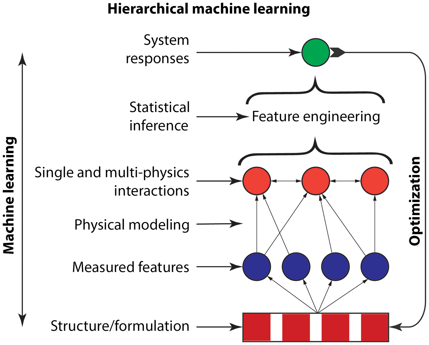
A combination of the prior reviewed approaches for embedding domain knowledge into systems has led to another ML approach, hierarchical machine learning (HML). Unlike PIML, HML incorporates physical domain knowledge through utilizing equations to predict the physical interactions that determine the properties or responses of a complex material system. True for all methods of embedding domain knowledge, the appropriate selection of physical interactions driving a system must at least include the essential descriptors behind any experiment. HML is a methodology that has been successfully implemented to extremely small datasets with the appropriate descriptor selections. The first implementation of HML, as described by Menon et al.,[Reference Menon, Gupta, Perkins, DeCost, Budwal, Rios, Zhang, Póczos and Washburn71] embedded domain knowledge into polymer dispersants to probe their effect in a cement-based system. Magnesium oxide is a popular nonsetting model of portland cement and dispersant design was the first system modeled using HML.[Reference Hirata, Ye, Branicio, Zheng, Lange, Plank and Sullivan72] The generic model of an HML system is shown in Fig. 7.
Akin to the hierarchical approach shown in Fig. 1, HML parameterizes a complex system in terms of either system structure or formulation. A bottom layer of observed features is directly measured. This bottom layer is related to the middle layer through embedding domain knowledge into the system through physical equations. This bottom to middle layer allows for the embedding of system physics without it having to be learned in a blackbox approach. The middle layer is utilized as inputs into the statistical learning techniques, such as Lasso, with cross-terms included so that multi-physics interactions are accounted for. After learning, an equation based on physical interactions utilizing ML the upward movement is complete. The predicted equation can be reparamaterized in terms of the initial material structure or formulation on the bottom layer and optimized, as shown by the downward arrow.
A polymer dispersant used in cement systems is known as a superplasticizer. Superplasticizers are utilized to reduce yield stress without an increase in water addition, which reduces strength.[Reference Marchon, Juilland, Gallucci, Frunz and Flatt73] Individual measurements of adsorption (θ), zeta potential (ζ), sedimentation experiments (s), intrinsic viscosity (η), and the osmotic second virial, A2, were performed. Each of these individual measurments was related to the associated force through physical equations, which define how superplasticizers reduce yield stress within cementitious systems. For example, an increase in viscous force was assumed to vary linearly with free polymer concentration (c o) so that:

where $\lsqb {\eta_{{\rm pol}}\lpar \mathop{x}\limits^{\rightharpoonup} \rpar } \rsqb$ is parameterized in terms of polymer structure. Similar approaches were performed to represent measured properties in terms of physical interactions as shown in Fig. 8. A library of 10 polymers was utilized for the training set. Each polymer was parameterized in terms of their chemical group composition. Upon representing each polymer in terms of their respective force interactions through connecting the bottom to middle layer, an input of these interactions along with their squared and cross-terms was included in order to increase the system dimensionality and incorporate multi-physics interactions into the hypothesis-space of the material. The selected regression technique utilized was a regularized linear regression, Lasso.
The degree of polymer adsorption, θ, onto cement particles is calculated through a Freundlich fit to experimental data at various polymer concentrations, C i. The adsorbed polymer, where negatively charged polymer chains attract to the positively charged portion of cement particles, induces dispersion through both electrostatic effects, ζ pol, as fit to zeta potential measurements and electrosteric effects, s pol, as fit to sedimentation experiments. Free polymer induces solvent-mediated dispersing effects through both osmotic forces, π pol, as fit utilizing the second virial (A 2) as calculated through vapor pressure osmometry measurements and viscous forces, η pol, as fit to intrinsic viscosity measurements.

Lasso has the added benefit of a natural form of feature selection in order to reduce the final predicted regression to a line of only the physical interactions most contributing toward dispersibility effects. The predicted equation resulted in an equation for yield stress:

After solving for the regression, optimization was performed in order to parameterize chemical composition in terms of superplasticizer structure. The optimized polymer structure was found to correspond with a novel polymer, a polycarboxylate-grafted lignosulfonate. The synthesized polymer approached reductions in yield stress similar to those of the leading class of superplasticizers, polycarboxylate ethers, showing that embedded physical equations within ML are capable of learning fits and optimizing systems.
In a continuation of this research, HML was also shown to recognize subtle fluctuations in superplasticizer action for variations in the MgO system. Metakaolin (MK) is a calcined clay additive for improved cement strength. However, MK decreases cement workability.[Reference Ding and Li74] As a follow-up to the MgO study, MK-Portland Cement (MK-PC) systems were studied to design an effective dispersant utilizing HML.[Reference Washburn, Menon, Childs, Poczos, Kurtis, Martirena, Favier and Scrivener75,Reference Menon, Childs, Poczós, Washburn and Kurtis76] A similar set of procedures was followed for the ML algorithm and optimization followed on the resulting force-driven equation as predicted by Lasso. The resulting Lasso equation discovered for slump (a direct measurement of yield stress) was:

It is interesting to note that in both systems, an increase of viscous force, η, was an important determinant in maximizing the slump. Primary mechanisms of superplasticizers focus mainly upon the electrostatic forces, ζ, and electrosteric forces, s.[Reference Yoshioka, Sakai, Daimon and Kitahara77] Upon optimization, a novel styrene sulfonate-methacrylic acid-poly(ethylene glycol) methacrylate copolymer was synthesized. In line with the Lasso prediction, this optimized polymer resulted in having a higher intrinsic viscosity than any of the training set. The discovery of forces being more important than thought through human intuition illustrates one benefit of incorporating domain knowledge into a system. The synthesized polymer came close to the performance of commercial PCEs in MK-PC systems, but interestingly had poor performance within pure PC. This demonstrates that HML was able to account for the changes in the underlying forces of dispersion caused by the addition of MK showing one of the benefits of incorporating physical equations into the algorithm.
Future directions
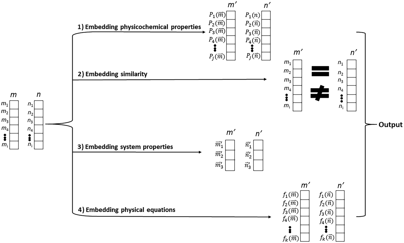
It has been shown that embedding domain knowledge into material systems allows learning physical interactions on small datasets. This knowledge can be incorporated into ML algorithms through the use of the correct data representation as shown in Fig. 9. One future prospect in research to allow improvement and usefulness will be on transfer learning. Transfer learning would allow for learning on one system similar to another and have the added benefit of increasing the size of the dataset through learning on similar systems. Figure 10 shows the theory consistent between physical and statistical relationships.
A common representation for a material or formulation is as a vector representing the structure or makeup of the system. The original vectors for materials m and n are shown through the four pathways of data representation which were discussed in this review for embedding domain knowledge into complex material systems to form transformed vectors m′ and n′. Method 1 represents the materials in the form of computational or experimental properties, P(x), for the original material. Method 2 represents the vectors through finding a (di)similarity metric to compare the two. Method 3 represents the vectors through a direct transformation of the x components in order to embed properties such as invariance. Method 4 represents the original material in terms of physical interactions utilizing known physical equations. These transformed vectors are utilized as the features for ML techniques to learn an associated output.

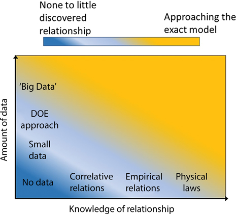
The goal of modeling a complex system is to predict the best relation possible. Knowing the physical laws of the system and interactions between the features allows an analytical model to be proposed based on physics alone, as shown on the horizontal axis. Statistics can also allow for the prediction of a good model if sufficient data are collected as is shown on the vertical axis. For many complex systems, neither of these is achievable. By having a combination of both physical and statistical modeling, a good model is able to be predicted and illustrates the importance of embedding physical knowledge into a system.

For systems following similar physical relations, introducing statistics from prior ML studies could easily be remodeled in the new system. Figure 11 shows an adapted schematic from Hutchinson et al.[Reference Hutchinson, Antono, Gibbons, Paradiso, Ling and Meredig78] showing three techniques of transfer learning. This methodology has already been studied in QC applications of ML where small molecules were studied to understand relations in larger molecules, an example of multi-task transfer learning.[Reference Hutchinson, Antono, Gibbons, Paradiso, Ling and Meredig78,Reference Welborn, Cheng and Miller79] The ultimate goal for such studies with proper relations being embedded or learned through ML would be a universal reactive force field.[Reference Bartók, De, Poelking, Bernstein, Kermode, Csányi and Ceriotti80] QC has also utilized approaches of difference transfer learning where computational and experimental outputs are compared to predict a system output. Learning on the difference allows for variables to be found to fit a closure model. Such learning techniques have been studied on the prediction of turbulence flow.[Reference Parish and Duraisamy81]
Schematics for three types of transfer learning. (a) Multi-task transfer learning is when one model is learned to fit multiple systems. (b) Latent variable transfer learning is a technique where a latent domain variable is learned on one system and included as a feature for predicting the output of another system. (c) Difference transfer learning is a technique where training data are relabeled as the difference between features and a model is learned from this difference.

One issue that needs to be resolved in transfer learning is ensuring proper physics are embedded as the system is changed. Akin to the example of the truck driving across a river in winter, crystal deformations vary from a Cauchy–Born relation as temperature changes. These simulations were all performed at 0 K, and utilizing the regression obtained through training would result in poor deformation prediction at higher temperatures. It would be necessary to embed domain knowledge, which predicts a temperature relation. Utilizing a latent variable transfer learning approach could be one possibility in accomplishing this, as temperature effects could be learned through a latent variable. Determining the appropriate transfer learning approach for each domain knowledge ML technique may be a system-independent approach that again may require prior human knowledge with test and error approaches. If the physics in the interactions within the complex system do not change, multi-task learning may be the best technique to utilize. If the underlying physics do change, then other transfer learning techniques may need to be considered.
Conclusion
In the utilization of ML for science, physical theories can be utilized to improve models in conjunction with data as opposed to being relearned through only the incorporation of data. ML approaches for physical systems have quickly developed to incorporate scientific fields. Starting with purely statistical analysis of raw data, techniques have progressed over time to include expert knowledge, incorporate physical parameters as features, incorporate metrics of correlation between data, discover physical laws which model simple systems, and now approach a level as to embed multiple physical laws to predict outputs from complex systems. With complex materials being expensive, time-intensive systems on which to test, methods to improve the cost-effectiveness and reduce the time to find an optimized system are essential. Deploying these hybrid physical–statistical approaches, more accurate modeling and relationships can be extrapolated and understood using domain knowledge-embedded machine learning.
Acknowledgments
Support from the National Science Foundation (CBET-1510600) is gratefully acknowledged.