2. Dynamic modeling of space manipulators

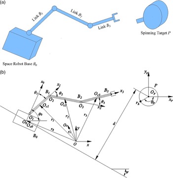
A planar three-link space manipulator and a spinning target are shown in Fig. 1. The space manipulator consists of a free-floating rigid base B ₀ (chaser) and rigid bars B ₁, B ₂, B ₃. P is the target to be captured. $Oxy$ is the inertial coordinate frame of the system. And the base moves along its trajectory with a velocity $\textbf{v}$ . It is assumed that the mass center of the whole system and that of the base satellite coincide for any configuration of the manipulator [Reference Zong, Emami, Luo and Electron38]. Due to the large radius of curvature of the trajectory, the trajectory in a short period can be approximately regarded as a straight line. The target is a cylindrical object revolving around its mass center with angular velocity ${\dot \theta _p}$ , and the distance between its handle and its mass center is r _h. The trajectory of the base is inclined at an angle $\psi $ relative to the x axis, and the distance between the mass center of the target and the base’s trajectory is d. At the point of interception, the relative velocity between the manipulator end-effector and the handle of the target is $\Delta \textbf{v}$ . ${O_i}{x_i}{y_i}$ is the local coordinate frame of ${B_i}(i = 0,1,2,3)$ . O ₀ is coincident with the mass center O _c0 of B ₀, ${O_{ci}}$ is the mass center of ${B_i}(i = 0,1,2,3)$ , ${O_i}(i = 1,2,3)$ is the rotational center of the revolute joint between ${B_{i - 1}}$ and ${B_i}(i = 0,1,2,3)$ , ${x_i}(i = 1,2,3)$ is the symmetry axis of B _i , respectively. Other symbols are defined as follows:

1. e _i Unit vector along the x _i axis;

2. l ₀ Distance between points O ₀ and O ₁;

3. l_i Length of B _i (i = 1,2,3) along the x _i axis;

4. b_i Distance between point ${O_i}(i = 1,2,3)$ and the mass center O _Ci (i = 1,2,3);

5. m _i Mass of B _i (i = 0,1,2,3);

6. J_i Inertial moment of B _i with respect to its mass center O _Ci (i = 0,1,2,3);

7. O _c Mass center of the system;

8. θ ₀ Attitude angle of x ₀ axis relative to x axis;

9. θ _i Joint angles of B _i (i = 1,2,3);

10. r _i Position vector of the mass center O _Ci of B _i (i = 0,1,2,3) in (O-xy) frame, ${r_i} = {[{x_i}\quad {y_i}]^{\textrm{T}}}$ ;

11. T _i The kinetic energy of B _i (i = 0,1,2,3)

12. $\dot{( \ )}$ The first time derivative of $(\ )$ ;

13. $\ddot{( \ )}$ The second time derivative of $(\ )$ ;

14. $\hat{(\ )}$ The estimate of $(\ )$ ;

15. $\left[\left(\,\,\,\right)\right]$ The allowable value of $(\,)$ .

From Fig. 1, r _i (i = 1,2,3) are

(1) \begin{equation}\textbf{r}_i=\textbf{r}_0+\sum\limits_{j = 0}^{i - 1} {{l_j\textbf{e}_j}}+b_i\textbf{e}_i\end{equation}

Differentiating Eq. (1) with respect to time t, ${\dot{\textbf{r}}_i}$ (i = 1,2,3) are

(2) \begin{equation}\dot{\textbf{r}}_i=\dot{\textbf{r}}_0+\sum\limits_{j = 0}^{i - 1} {{l_j\dot{\textbf{e}}_j}}+b_i\dot{\textbf{e}}_i\end{equation}

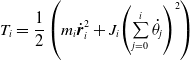
Then the manipulator system’s total kinetic energy T is

(3) \begin{align}T = \sum\limits_{i = 0}^3 {{T_i}} \end{align}

where ${T_i} = \dfrac{1}{2}\left( {{m_i}\dot{\textbf{r}}_i^{\rm{2}} + {J_i}{{\left( {\sum\limits_{j = 0}^i {{{\dot \theta }_j}} } \right)}^2}} \right)$ .

Figure 1.

A free-floating space manipulator and a spinning target.

The microgravity is ignored, and the potential energy of the system V is 0. Then the system’s Lagrangian L = T-V= T and the Euler–Lagrange dynamic equations of the space manipulator are derived as [Reference Song39]

(4) \begin{equation}\textbf{D}(\textbf{q})\ddot{\textbf{q}}+\textbf{H}(\textbf{q},\dot{\textbf{q}})\dot{\textbf{q}}=\boldsymbol{\tau}\end{equation}

where $\textbf{q} = [\begin{array}{c@{\quad}c@{\quad}c@{\quad}c@{\quad}c@{\quad}c} {{x_0}} & {{y_0}} & {}{{\theta _0}} & {{\theta _1}} & {}{{\theta _2}} & {{\theta _3}} \end{array} ]^{\rm{T}}$ is the generalized coordinates, $\textbf{D}(\textbf{q})\in\textbf{R}^{6\times6}$ denotes the symmetric inertial matrix, $\textbf{H}(\textbf{q},\dot{\textbf{q}})\in\textbf{R}^{6\times6}$ is the Coriolis/centrifugal matrix, ${\boldsymbol{\tau}} = {\left[{\textbf{0}}\;\;\;{\boldsymbol{\tau}}_l^{\textrm{T}}\right]^{\textrm{T}}} \in {{\textbf{R}}^{6 \times 1}}$ , ${{\boldsymbol{\tau}}_l} = {[{\tau _1}\;\;\;{\tau _2}\;\;\;{\tau _3}]^{\textrm{T}}} \in {{\textbf{R}}^{3 \times 1}}$ , ${{\tau }_i}(i = 1,2,3)$ is the input torque of joint i.

3. RNS motion planning of space manipulators

3.1. RNS motion planning algorithm

By partitioned matrix, Eq. (4) is rewritten as

(5) \begin{align}\left[\begin{array}{c@{\quad}c} {{{\textbf{D}}_{bb}}} & {}{{{\textbf{D}}_{bl}}} \\[4pt] {{{\textbf{D}}_{lb}}} & {}{{{\textbf{D}}_{ll}}}\end{array} \right] \left[ \begin{array}{c} {{{\ddot{\textbf{q}}}_b}} \\[4pt] {{{\ddot{\textbf{q}}}_l}} \end{array} \right] + \left[ \begin{array}{c} {{{\textbf{H}}_b}} \\[4pt] {{{\textbf{H}}_l}} \end{array} \right] \left[ \begin{array}{c} {{{{\dot{\textbf{q}}}}_b}} \\[4pt] {{{{\dot{\textbf{q}}}}_l}} \end{array} \right] = \left[ \begin{array}{c} \textbf{0} \\[4pt] {{\boldsymbol{\tau} _l}} \end{array} \right]\end{align}

where $\textbf{D}_{bb}\in\textbf{R}^{3\times3}$ is the base inertia matrix, $\textbf{D}_{ll}\in\textbf{R}^{3\times3}$ is the arm inertial matrix, $\textbf{D}_{bl}\in\textbf{R}^{3\times3}$ is the base-arm coupling inertia matrix, $\textbf{q}_{b} = {[ {{x_0}}\quad {}{{y_0}}\quad {}{{\theta _0}} ]^{\textrm{T}}}$ , $\textbf{q}_{l} = {[{{\theta _{\rm{1}}}} \quad {}{{\theta _{\rm{2}}}}\quad {}{{\theta _{\rm{3}}}} ]^{\textrm{T}}}$ .

Integrating the first row of Eq. (5), the system’s linear momentum P and angular momentum L [Reference Yu, Guo and Zhang40] are

(6) \begin{align}\left(\begin{array}{c}{\textbf{P}}\\[3pt]{\textbf{L}}\end{array}\right) = \int \textbf{0}dt = {{\textbf{D}}_{bb}}{{\dot{\textbf{q}}}_b} + {{\textbf{D}}_{bl}}{{\dot{\textbf{q}}}_l} = const\end{align}

where ${{\textbf{D}}_{bb}}{{\dot{\textbf{q}}}_b}$ is the base momentum, ${{\textbf{D}}_{bl}}{{\dot{\textbf{q}}}_l}$ is the coupling momentum generated by the arm motion. Introduce ${\textbf{L}_l} = {{\textbf{D}}_{bl}}{{\dot{\textbf{q}}}_l}$ and the derivative of ${\textbf{L}_l}$ is

(7) \begin{equation}\dot{{\textbf{L}_l}}={\textbf{F}_l}={{\textbf{D}}_{bl}}{{\ddot{\textbf{q}}}_l} + {{\dot{\textbf{D}}}_{bl}}{{\dot{\textbf{q}}}_l}\end{equation}

where ${\textbf{F}_l}$ is the reaction forces induced on the base from the motion of the arm.

When coupling momentum is constant, ${{\textbf{F}_l}} \equiv {\textbf{0}}$ . Then the arm’s motion leads to no reaction force or torque to the base. When the number of the degree of freedom of the manipulator is greater than that of the base coordinates, the manipulator joint rates satisfy [Reference Yu, Guo and Zhang40]

(8) \begin{align}{{{{\dot{\textbf{q}}_l}}}} = {\textbf{D}}_{bl}^ + {{\textbf{L}_l}} + \left( {\textbf{I}- {\textbf{D}}_{bl}^ + {\textbf{D}_{bl}}} \right){\boldsymbol\xi} \end{align}

where ${(\,)^ + }$ is the pseudo-inverse of $(\,)$ , $\textbf{I}\in\textbf{R}^{3\times3}$ represents the identity matrix, $({\textbf{I}} - {\textbf{D}}_{bl}^ + {{\textbf{D}}_{bl}})$ is the mapping onto the null space of ${\textbf{D}_{bl}}$ , and ${\boldsymbol{\xi }} \in {{\textbf{R}}^{3 \times 1}}$ represents an arbitrary vector. This inertial null space is called the “zero reaction space.” When the coupling momentum ${\textbf{L}_l} = {\textbf{0}}$ , Eq. (9) is obtained

(9) \begin{align}{\left( {{{{\dot{\textbf{q}}}}_l}} \right)_{RNS}} = \left( {{\textbf{I}} - {\textbf{D}}_{bl}^ + {{\textbf{D}}_{bl}}} \right)\boldsymbol\xi \end{align}

The base’s attitude is merely considered and the modified coupling inertial matrix ${{{\tilde{\textbf{D}}}}_{bl}} = [{D}_{34}\ \ {}{D}_{35}\ \ {}{D}_{36} ]$ [Reference Brahmi, Driscoll, Laraki and Brahmi32] is defined, then Eq. (9) is transformed into

(10) \begin{align}{\left( {{{{\dot{\textbf{q}}}}_l}} \right)_{RNS}} = \left( {\textbf{I} - \tilde {\textbf{D}}_{bl}^ + {\tilde {\textbf{D}}_{bl}}} \right)\boldsymbol\xi \end{align}

The reactionless joint trajectories can be obtained by integrating Eq. (10).

3.2. Vector norm constraint algorithm of RNS planning

$\boldsymbol\xi $ can be properly chosen to ensure constraints of the joint angular velocities and joint angular accelerations are satisfied. Define 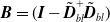${\textbf{B}} = (\textbf{I}- {{\tilde{\textbf{D}}}}_{bl}^ + {{{\tilde{\textbf{D}}}}_{bl}})$ and utilize Eq. (10), joint angular velocities ${\left( {{{{{{\dot{\textbf{q}}}}}}_l}} \right)_{int}}$ and joint angular accelerations ${\left( {{{{{\ddot{\textbf{q}}}}}_l}} \right)_{int}}$ at the interception point are

(11) \begin{align}\left\{\!\begin{array}{l} \left\| \left( {\dot{\textbf{q}}}_{l} \right)_{int}\right\| = \left\| {{\textbf{B}}}\boldsymbol\xi \right\|\\[5pt]\left\| \left( {\ddot{\textbf{q}}}_{l} \right)_{int}\right\| = \left\| \dfrac{d{\textbf{B}}}{dt} \boldsymbol\xi \right\|\end{array}\right.\end{align}

Extending it to the entire manipulation process, then joint angular velocities ${({{\dot{\textbf{q}}}_l})_{RNS}}$ and joint angular accelerations ${({\ddot{\textbf{q}}_l})_{RNS}}$ of RNS are

(12) \begin{align}\left\{\!\begin{array}{l} \left\| \left( {\dot{\textbf{q}}}_{l} \right)_{RNS}\right\| = \left\| {{\textbf{B}}}\boldsymbol\xi \right\|\\[5pt]\left\| \left( {\ddot{\textbf{q}}}_{l} \right)_{RNS}\right\| = \left\| \dfrac{d{\textbf{B}}}{dt} \boldsymbol\xi \right\|\end{array}\right.\end{align}

By Eq. (7), the reaction forces onto the base from the arm are

(13) \begin{align}{\textbf{F}_{RNS}} = {{\textbf{D}}_{bl}}{\left( {{{{\ddot{\textbf{q}}}}_l}} \right)_{RNS}} + {\dot{\textbf{D}}_{bl}}{\left( {{{{\dot{\textbf{q}}}}_l}} \right)_{RNS}} = \left(\begin{array}{c}{F_x}\\[3pt]{F_y}\\[3pt]{T_z}\end{array}\right)\end{align}

where ${F_x}$ and ${F_y}$ are reaction forces, ${T_z}$ is the corresponding reaction torque.

Substituting ${\left( {{{{{{\dot{\textbf{q}}}}}}_l}} \right)_{RNS}} = {\textbf{B}}\boldsymbol{\xi }$ and ${\left( {{{{{\ddot{\textbf{q}}}}}_l}} \right)_{RNS}} = \dfrac{d{\textbf{B}}}{dt}\boldsymbol\xi$ into Eq. (13), then combining Eq. (12), Eq. (14) is derived

(14) \begin{align}\left\{\begin{array}{l} \left\| \left( {\dot{\textbf{q}}}_{l} \right)_{RNS}\right\|_{2} = \left\| {{\textbf{B}}}\boldsymbol\xi \right\|_{2}\\[5pt]\left\| \left( {\ddot{\textbf{q}}}_{l} \right)_{RNS}\right\|_{2} = \left\| \dfrac{d{\textbf{B}}}{dt} \boldsymbol\xi \right\|_{2}\\[9pt]\left\| {{\textbf{F}}}_{RNS}\right\|_{2} = \left\|\left({\textbf{D}}_{bl} \dfrac{d{\textbf{B}}}{dt} + \dot{\textbf{D}}_{bl} {\textbf{B}}\right)\boldsymbol\xi \right\|_{2}\end{array}\right.\end{align}

where ${\left\| {} \right\|_2}$ is the Euclidean norm. Then

(15) \begin{align}\left\{\begin{array}{l} \left\| \left( {\dot{\textbf{q}}}_{l} \right)_{RNS}\right\|_{2}^{2} = \boldsymbol{\xi}^{\textrm{T}}{\textbf{A}}_1 \boldsymbol{\xi}\\[5pt]\left\| \left( {\ddot{\textbf{q}}}_{l} \right)_{RNS}\right\|_{2}^{2} = \boldsymbol{\xi}^{\textrm{T}}{\textbf{A}}_2 \boldsymbol{\xi}\\[9pt]\left\| {{\textbf{F}}}_{RNS}\right\|_{2}^{2} = \boldsymbol{\xi}^{\textrm{T}}{\textbf{A}}_3 \boldsymbol{\xi}\end{array}\right.\end{align}

where ${{\textbf{A}}_i} \in {{\textbf{R}}^{3 \times 3}}(i = 1,2,3)$ are obtained by expanding the right side of Eq. (14). Then $\boldsymbol{\xi }$ can be calculated by Eq. (15).

The reactionless path of the manipulator can be obtained by integrating Eq. (10) from ${t_f}$ to ${t_0}$ , in which ${t_f}$ is the time of interception and ${t_0}$ is the starting time of manipulation. The initial states of the integral are joint angles of the manipulator at the moment of interception, which should be obtained first. This can be obtained by inverse kinematics [Reference Song39].

At the moment of interception, the velocity ${\textbf{v}_e}$ of the end-effector should be the same as the velocity ${{\textbf{v}}_h}$ of the target handle. In practice, $\left\| {{{\textbf{v}}_e} - {{\textbf{v}}_h}} \right\| \le [\Delta v]$ is ensured. The end-effector’s velocity is

(16) \begin{align}{{\textbf{v}}_e} = {{\textbf{v}}_{O0}} + {{\textbf{v}}_{eO0}}\end{align}

where ${{\textbf{v}}_{O0}}$ is the velocity of O ₀, ${{\textbf{v}}_{eO0}}$ is the relative velocity of the end-effector relative to O ₀.

(17) \begin{align}{{\textbf{v}}_{eO0}} = {\textbf{J}}{{\dot{\textbf{q}}}_\theta }\end{align}

where ${{\dot{\textbf{q}}}_\theta } = {[{\dot \theta _0}\quad {\dot \theta _1}\quad {\dot \theta _2}\quad {\dot \theta _3}]^{\textrm{T}}}$ , ${\textbf{J}}$ is Jacobian matrix.

(18) \begin{align}{\textbf{J}} = \left[\begin{array}{l} - {l_0}{s_0} - {l_l}{s_{01}} - {l_2}{s_{012}} - {l_3}{s_{0123}}\quad - {l_1}{s_{01}} - {l_2}{s_{012}} - {l_3}{s_{0123}}\quad - {l_2}{s_{012}} - {l_3}{s_{0123}} \quad - {l_3}{s_{0123}} \\[6pt]{l_0}{c_0} + {l_1}{c_{01}} + {l_2}{c_{012}} + {l_3}{c_{0123}}\qquad {l_1}{c_{01}} + {l_2}{c_{012}} + {l_3}{c_{0123}}\qquad {l_2}{c_{012}} + {l_3}{c_{0123}}\qquad {l_3}{c_{0123}} \end{array}\right]\end{align}

where ${s_0} = \sin\! ({\theta _0})$ , ${s_{01}} = \sin\! ({\theta _0} + {\theta _1})$ , ${s_{012}} = \sin \left({\theta _0} + {\theta _1} + {\theta _2}\right)$ , ${s_{0123}} = \sin \left({\theta _0} + {\theta _1} + {\theta _2} + {\theta _3}\right)$ , ${c_0} = \cos \left({\theta _0}\right)$ , ${c_{01}} = \cos \left({\theta _0} + {\theta _1}\right)$ , ${c_{012}} = \cos \left({\theta _0} + {\theta _1} + {\theta _2}\right)$ , ${c_{0123}} = \cos \left({\theta _0} + {\theta _1} + {\theta _2} + {\theta _3}\right)$ .

The velocity ${{\textbf{v}}_h}$ of the target handle is found from

(19) \begin{align}{{\textbf{v}}_h} = \left[\begin{array}{c}{{\dot x}_h}\\[4pt] {\dot y}_h \end{array}\right] = \left[\begin{array}{c} {{{\dot x}_P} - {r_h}{{\dot \theta }_P}\sin {\theta _P}}\\[4pt] {{\dot y}_P} + {r_h}{\dot \theta _P}\cos {\theta _P} \end{array} \right]\end{align}

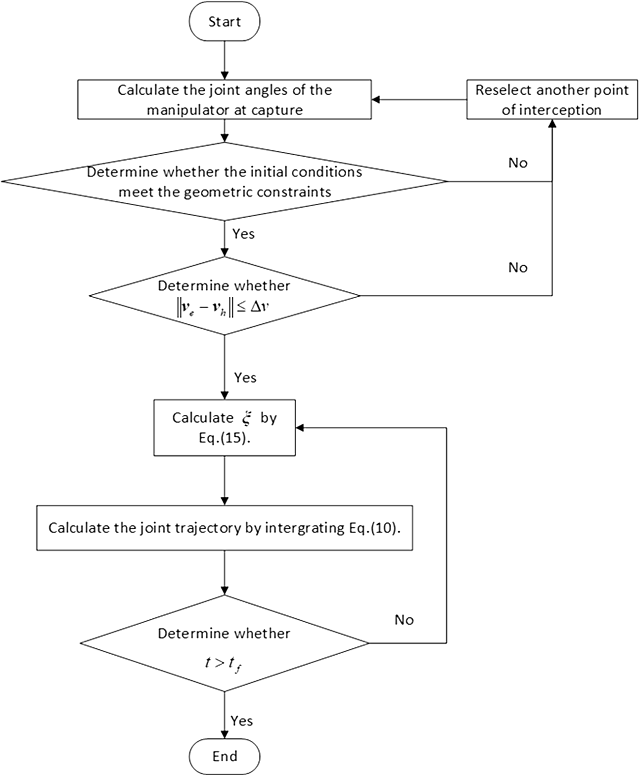
The main steps of the vector norm constraint algorithm of RNS Planning are shown in Fig. 2.

Figure 2.

The flow chart of the vector norm constraint algorithm of RNS planning.

4. TDE-based augmented adaptive sliding mode control design

Introduce matrix ${{\textbf{D}}_I}{\rm{ = diag(}}{{D}_{I{\rm{1}}}}{\rm{,}} \cdots {{D}_{Ii}}{\rm{,}}{\kern 1pt} \cdots ,{\kern 1pt} {\kern 1pt} {{D}_{I{\rm{6}}}}{\rm{)}}$ , the dynamics Eq. (4) is rewritten as

(20) \begin{align}\boldsymbol\tau = {{\textbf{D}}_I}{\ddot{\textbf{q}}} + {\textbf{h}}\end{align}

(21) \begin{align}{\textbf{h}} = \left( {{\textbf{D}}({\textbf{q}}) - {{\textbf{D}}_I}} \right)\ddot{\textbf{q}} + \textbf{H}\left( {{\textbf{q}},{\dot{\textbf{q}}}} \right){\dot{\textbf{q}}}\end{align}

where ${{\textbf{D}}_I}$ is the estimate of the inertia matrix ${\textbf{D}}$ , ${{D}_{Ii}}(i = 1, \cdots ,6)$ are given constants.

Define the augmented output error vector

(22) \begin{align}{\textbf{e}} = {{\textbf{q}}_d} - {\textbf{q}}\end{align}

(23) \begin{align}\dot{\textbf{e}} = {{\dot{\textbf{q}}}_d} - {\dot{\textbf{q}}}\end{align}

where ${{\textbf{q}}_d} = {\left[ {{x_0}} \quad {}{{y_0}} \quad {}{{\theta _0}}\quad {}{{\textbf{q}}_{ld}^{\textrm{T}}} \right]^{\textrm{T}}}$ and ${{{{\dot{\textbf{q}}}}}_d} = {\left[{{{\dot x}_0}} \quad {}{{{\dot y}_0}}\quad {}{{{\dot \theta }_0}} \quad {}{{{{\dot{\textbf{q}}}}}_{ld}^{\textrm{T}}} \right]^{\textrm{T}}}$ are the augmented desired trajectories and the augmented desired velocities, ${{\textbf{q}}_{ld}} = {[{{\theta _{1d}}} \quad {}{{{\theta }_{2d}}}\quad {}{{{\theta }_{{\rm{3}}d}}} ]^{\textrm{T}}}$ , ${{{{\dot{\textbf{q}}}}}_{ld}} = {[ {{{\dot \theta }_{1d}}}\quad {}{{{{\dot \theta }}_{2d}}} \quad {}{{{{\dot \theta }}_{{\rm{3}}d}}} ]^{\textrm{T}}}$ . Then the augmented output error vector ${\textbf{e}}$ is

(24) \begin{align}{\textbf{e}} = \left[\textbf{0}\quad {\textbf{e}}_l^{\textrm{T}} \right]^{\textrm{T}}\end{align}

where ${{\textbf{e}}_l} = {{\textbf{q}}_{ld}} - {{\textbf{q}}_l}$ .

The sliding surface s is chosen as

(25) \begin{align}{\textbf{s}} = \dot{\textbf{e}} + {\boldsymbol\Lambda _1}{\textbf{e}} + {\boldsymbol\Lambda _2}{\boldsymbol{\rho}}\end{align}

where ${{\boldsymbol{\Lambda }}_{\rm{1}}},{{\boldsymbol{\Lambda }}_{\rm{2}}} \in {\textbf{R}^{6 \times 6}}$ are positive definite diagonal matrices, ${{\boldsymbol{\Lambda }}_1} = {\rm{diag(}}{{\lambda }_{11}}, \cdots ,{{\lambda }_{1i}}, \cdots ,{{\lambda }_{16}}{\rm{)}}$ , ${{\boldsymbol{\Lambda }}_2} = {\rm{diag(}}{{\lambda }_{21}}, \cdots ,{{\lambda }_{2i}}, \cdots ,{{\lambda }_{26}}{\rm{)}}$ , ${{\lambda }_{ji}} \gt 0(j = 1,2;\,i = 1, \cdots ,6)$ , ${\textbf{s}} = {[ {{{s}_1}}\ \ {} \cdots \ \ {}{{{s}_i}} \ \ {} \cdots\ \ {}{{{s}_6}} ]^{\textrm{T}}}$ , ${\boldsymbol{\rho}} = $ ${[{{{\rho }_1}} \ {} \cdots \ {}{{{\rho }_i}}\ {} \cdots\ {}{{{\rho }_6}} ]^{\textrm{T}}}$ , ${{\rho }_i}(i = 1\sim 6)$ are

(26) \begin{align}{\rho _i} = \left\{\begin{array}{ll} sig{{({e_i})}^{\alpha_{1i}}}, & {}{s_{1i}} = 0 \vee \left({{{s}}_{1i}} \ne {\rm{0}} \wedge |e_i| \geq {\phi _i}\right)\\[5pt]{\eta _{1i}}{e_i} + {\eta _{2i}}f({e_i}), & {}{s_{1i}} \ne 0 \wedge |e_i| \lt {\phi _i}\end{array}\right.\end{align}

(27) \begin{align}f\!\left( {{e_i}} \right) = \left( 1 + {k_{1i}}\cos \left(\frac{ \pi e_i}{2{\phi _i}} \right) \right)sig{\left( {{e_i}} \right)^{{\alpha _{2i}}}}\end{align}

where ${s_{1i}} = {\dot{{e}}_i} + {\lambda _{1i}}{e_i} + {\lambda _{2i}}sig{({e_i})^{{\alpha _{1i}}}}$ , $0.5 \lt {\alpha _{{\rm{1}}i}} \lt 1$ , $1 \lt {\alpha _{2i}} \lt 2$ , ${\phi _i}$ are positive constants, $sig{({e_i})^{{\alpha _{ji}}}} = {\left| {{e_i}} \right|^{{\alpha _{ji}}}}{\mathop{\rm sgn}} ({e_i})$ , $j = 1,2$ , ${\mathop{\rm sgn}} ({e_i})$ , ${\eta _{1i}}$ and ${\eta _{{\rm{2}}i}}$ are

(28) \begin{align}{\mathop{\rm sgn}}\! \left( {{e_i}} \right) = \left\{\begin{array}{l@{\quad}l}1, & {e_i} \gt 0\\[3pt]0, & {e_i} = 0\\[3pt]- 1, & {e_i} \lt 0\end{array}\right.\end{align}

(29) \begin{align}\eta_{1i} = \left( \dfrac{{\alpha _{2i}} - \dfrac{\pi {k_{1i}}}{2} - {\alpha _{1i}}}{{\alpha_{2i}} - \dfrac{\pi {k_{1i}}}{2} - 1} \right){\phi _i}^{{\alpha _{1i}} - 1},{\eta _{2i}}=\left( \frac{{\alpha _{1i}} - 1}{\alpha _{2i} - \dfrac{\pi {k_{1i}}}{2} - 1} \right){\phi _i}^{{\alpha _{1i}} - {\alpha _{2i}}}\end{align}

where ${\rm{0}} \le {k_{1i}} \lt \dfrac{2({\alpha _{2i}} - 1)}{\pi}$ .

The first time derivative of ${{\rho }_i}$ is

(30) \begin{align}{\dot \rho _i} = \left\{\begin{array}{ll} {{\alpha _{{\rm{1}}i}}{{\left| {{e_i}} \right|}^{{\alpha _{1i}} - 1}}{\dot{e}_i},} & {}{{s_{1i}} = 0 \vee \left( {{s_{1i}} \ne 0 \wedge \left| {{e_i}} \right| \ge {\phi _i}} \right)}\\[5pt] {{\eta _{1i}}{\dot{e}_i} + F\!\left( {{e_i}} \right),} & {}{{s_{1i}} \ne 0 \wedge \left| {{e_i}} \right| \lt {\phi _i}} \end{array} \right.\end{align}

(31) \begin{align}F\left( {{e_i}} \right) = {\eta _{2i}}{\alpha _{2i}}\left( {1 + {k_{1i}}{\rm{cos}}\!\left( {{{\pi {e_i}} \over {2{\phi _i}}}} \right)} \right){\left| {{e_i}} \right|^{{\alpha _{2i}} - 1}}{\dot{e}_i} - {\eta _{2i}}{k_{1i}}{\rm{sin}}\!\left( {{{\pi {e_i}} \over {2{\phi _i}}}} \right){sig}{\left( {{e_i}} \right)^{{\alpha _{2i}}}}{{\pi {\dot{e}_i}} \over {2{\phi _i}}}\end{align}

Then the following approaching law $\boldsymbol\Delta $ is proposed

(32) \begin{align}\boldsymbol\Delta = {{\textbf{K}}_1}s - {{\textbf{K}}_2}sig{({\textbf{s}})^\beta }\end{align}

where ${{\textbf{K}}_1}$ and ${{\textbf{K}}_{\rm{2}}}$ are diagonal matrices, ${{\textbf{K}}_1} = {\rm{diag(}}{\mu _{11}}, \cdots ,{\mu _{1i}}, \cdots ,{\mu _{16}}{\rm{)}}$ , ${{\textbf{K}}_2} = {\rm{diag(}}{\mu _{21}}, \cdots ,$ ${\mu _{2i}}, \cdots ,{\mu _{26}}{\rm{)}}$ , ${\mu _{ji}} \gt 0(j = 1,2;\, i = 1, \cdots ,6)$ , $0 \lt \beta \lt 1$ .

By augmentation approach, an augmented sliding mode controller (controller I) is proposed

(33) \begin{align}\boldsymbol\tau = {{\textbf{D}_I}}{\boldsymbol{\gamma}} + \hat{\textbf{h}}\left( {{\textbf{q}},{\dot{\textbf{q}}},\ddot{\textbf{q}}} \right) + \left[ {{\boldsymbol\varsigma ^{\textrm{T}}}\quad \bf{0}} \right]\end{align}

(34) \begin{align}\boldsymbol\gamma = {\ddot{\textbf{q}}_{\rm d}} + {\textbf{w}} + {{\textbf{K}}_1}{\textbf{s}} + {{\textbf{K}}_2}sig{({\textbf{s}})^\beta } + {\textbf{k}}\left| {\textbf{w}} \right|{\mathop{\rm sgn}} ({\textbf{s}})\end{align}

where ${{\hat{\textbf{h}}}}$ is the estimate of ${\textbf{h}}$ , ${\textbf{w}} = {{\boldsymbol{\Lambda }}_1}{\dot{\textbf{e}}} + {{\boldsymbol{\Lambda }}_2}{{\dot{\boldsymbol\rho}}}$ , ${\textbf{w}} = {[ {{w_1}} \quad {} \cdots \quad {}{{w_i}} \quad {} \cdots \quad {}{{w_6}} ]^{\textrm{T}}}$ , ${\textbf{k}} = diag({k_1}, \cdots,$ ${k_i}, \cdots ,{k_6})$ , ${{k}_i}(i = 1\sim 6)$ is given later. The vector $\boldsymbol\varsigma = {[{\varsigma _1}\ \ {\varsigma _2}\ \ {\varsigma _3}]^{\textrm{T}}}$ guarantees that the first three terms of the vector ${\boldsymbol{\tau}} = {[\textbf{0}\quad {\boldsymbol{\tau}}_l^{\textrm{T}}]^{\textrm{T}}}$ are always 0.

By the adaptive delay estimation technique, ${{\hat{\textbf{h}}}}({\textbf{q}},{{{\dot{\textbf{q}}}}},{{\ddot{\textbf{q}}}})$ is

(35) \begin{align}\hat{\textbf{h}}\left( {{\textbf{q}},{\dot{\textbf{q}}},\ddot{\textbf{q}}} \right) = {{\textbf{h}}_{t - L}} = {\boldsymbol\tau _{t - L}} - {{\textbf{D}}_I}{\ddot{\textbf{q}}_{t - L}}\end{align}

As the delay time $L$ is short enough, then

(36) \begin{align}{\textbf{h}} \approx {{\textbf{h}}_{t - L}}\end{align}

The acceleration ${{{\ddot{\textbf{q}}}}_{t - {\rm{L}}}}$ is calculated by

(37) \begin{align}{\ddot{\textbf{q}}_{t - L}} = {\frac{{{\textbf{q}}_t} - 2{{\textbf{q}}_{t - L}} + {{\textbf{q}}_{t - 2L}}}{{L^2}}}\end{align}

The estimation error ${{\tilde{\textbf{h}}}_t}$ is

(38) \begin{align}\tilde {\textbf{h}_t} = {{\textbf{h}}_t} - {\hat{\textbf{h}}_t} = {{\textbf{h}}_t} - {{\textbf{h}}_{t - L}} = {{\textbf{D}}_I}\left( {\boldsymbol{\gamma} - \ddot{\textbf{q}}} \right) + \left[ {{\boldsymbol\varsigma^{\textrm{T}}}\quad \textbf{0}} \right]\end{align}

Define the error $\boldsymbol\delta = {[ {{\delta _1}} \cdots {{\delta _i}} \cdots {{\delta _6}} ]^{\textrm{T}}}$ as

(39) \begin{align}\boldsymbol\delta = {{\textbf{D}}_I}^{ - 1}{\tilde{{\textbf{h}}}_t} = \boldsymbol{\gamma} - \ddot{\textbf{q}} + {{\textbf{D}}^{-1}_I}\left[ {{\boldsymbol\varsigma ^{\textrm{T}}}\quad \textbf{0}} \right]\end{align}

So long as Eq. (40) is satisfied, the system is stable.

(40) \begin{align}\left| {{\lambda _i}\left( {{{\textbf{D}}^{ - 1}}{{\textbf{D}}_I} - {{\textbf{I}}_6}} \right)} \right| \lt 1\end{align}

where ${{\textbf{I}}_6}$ is a 6-dimensional identity matrix, ${\lambda _i}({{\textbf{D}}^{ - 1}}{{\textbf{D}}_{\textbf{I}}} - {{\textbf{I}}_6})$ is the ith eigenvalue of the matrix $({{\textbf{D}}^{ - 1}}{{\textbf{D}}_{\textbf{I}}} - {{\textbf{I}}_6})$ , $i = 1\sim 6$ .

In order to decrease the TDE error, a larger constant needs to be chosen for ${D_{Ii}}$ [Reference Cho, Baek and Han41]. Larger ${D_{Ii}}$ will lead to serious chattering. Even worse, Eq. (40) may not be satisfied, which leads to instabilities [Reference Chang and Park29]. Therefore, the adaptive TDE technology was introduced. Assume ${\hat{\textbf{D}}} = {\rm{diag(}}{{\hat{D}}_1}, \cdots ,{{\hat{D}}_i}, \cdots ,{{\hat{D}}_6}{\rm{)}}$ is the adaptive estimated inertia matrix, the estimate ${\hat{D}_i}(i = 1\sim 6)$ are

(41) \begin{align}{\hat{D}_i} = {{D}_{Ii}}\left( {1 + {k_{2i}}{\sigma _i}} \right)\end{align}

where ${k_{2i}}(i = 1\sim 6)$ are positive constants, ${\sigma _i}(i = 1\sim 6) \ge 0$ are defined later.

Then the augmented adaptive sliding mode controller based on TDE (controller II) is

(42) \begin{align} {}{\boldsymbol{\tau}} & = {{\hat{{\textbf{D}}}\boldsymbol{\gamma} }} + {{\hat{\textbf{h}}}}\left( {{\textbf{q}},{{{\dot{\textbf{q}}}}},{{\ddot{\textbf{q}}}}} \right) + \left[ {{\boldsymbol\varsigma ^{\textrm{T}}}} {}\quad \textbf{0} \right]\nonumber \\[5pt] {} & = {\hat{\textbf{D}}}\left( {{{{{\ddot{\textbf{q}}}}}_d} + {\textbf{w}} + {{\textbf{K}}_1}{\textbf{s}} + {{\textbf{K}}_2}{sig}{{\left( {\textbf{s}} \right)}^\beta }} \right) + {{\hat{{\textbf{D}}}{\textbf{k}}}}\left| {\textbf{w}} \right|{\mathop{\rm sgn}}\! \left( {\textbf{s}} \right) + \left[ {{\boldsymbol{\varsigma} ^{\textrm{T}}}} \quad {}\textbf{0} \right] + {{\boldsymbol{\tau}}_{t - L}} - {\hat{\textbf{D}}}{{{{\ddot{\textbf{q}}}}}_{t - L}} \end{align}

Substituting Eq. (42) into Eq. (20), then we have

(43) \begin{align}\ddot{\textbf{q}} = {{\textbf{D}}_I}^{ - 1}\left( {\hat{\textbf{D}}\boldsymbol\gamma + \hat{\textbf{h}}\!\left( {{\textbf{q}},{\dot{\textbf{q}}},\ddot{\textbf{q}}} \right) + \left[ {{\boldsymbol\varsigma ^{\textrm{T}}}\quad \textbf{0}} \right] - {\textbf{h}}} \right)\end{align}

Define the Lyapunov function ${{V}_i}$

(44) \begin{align}{{V}_i} = {1 \over 2}{{s}_i}^2 + {{{{\tilde \sigma }_{i}}^2} \over {2{\upsilon _i}}}\end{align}

where ${\upsilon _i}$ is a positive constant, ${\tilde \sigma _i} = {\sigma _{i,{\rm{max}}}} - {\sigma _i} \ge 0$ , ${\sigma _{i,{\rm{max}}}}$ is the maximum of ${\sigma _i}$ , $i = 1\sim 6$ .

Differentiating Eq. (44) with respect to time t and utilizing $\textbf{w} = {{\boldsymbol{\Lambda }}_1}{\dot{\textbf{e}}} + {{\boldsymbol{\Lambda }}_2}{{\dot{\boldsymbol\rho}}}$ , Eqs. (25) and (43), ${{\dot V}_i}$ is

(45) \begin{align}{\dot V_i} & = {s_i}{s_i} + {\dfrac{{{\dot{\tilde{\sigma}}}_i}{{\tilde \sigma }_i}}{{v_i}}} = {s_i}\left( {{{\ddot e}_i} + {\mu _{1i}}{\dot{e}_i} + {\mu _{2i}}{{\dot{\rho}}_i}} \right) + {\dfrac{{{\dot{\tilde{\sigma}}}_i}{{\tilde \sigma }_i}}{{v_i}}} = s_{i} \left({\ddot{q}}_{id} - {\ddot{q}}_{i} + w_{i}\right) + {\dfrac{{{\dot{\tilde{\sigma}}}_i}{{\tilde \sigma }_i}}{{v_i}}}\nonumber\\[3pt] & = \left\{\begin{array}{l@{\quad}l}{s_i}\!\left( {{{\ddot{q}}_{id}} - {{D}_{Ii}}}^{ - 1}\left( {{{\hat{D}}_i}{\gamma _i} + {{\hat{h}}_i} + {\varsigma _i} - {h_i}} \right) + {{w_i}} \right) + {\dfrac{{{\dot{\tilde{\sigma}}}_i}{{\tilde \sigma }_i}}{{v_i}}} & i = 1,2,3\\[7pt]{s_i}\!\left( {{{\ddot{q}}_{id}} - {{D}_{Ii}}}^{ - 1}\left( {{{\hat{D}}_i}{\gamma _i} + {{\hat{h}}_i} - {h_i}} \right) + {{w_i}} \right) + {\dfrac{{{\dot{\tilde{\sigma}}}_i}{{\tilde \sigma }_i}}{{v_i}}} & i = 4,5,6\end{array} \right.\end{align}

${\sigma _{i,{\rm{max}}}}$ is a constant and ${\tilde \sigma _i} = {\sigma _{i,{\rm{max}}}} - {\sigma _i}$ , so ${{\dot{\tilde{\sigma}}} _i} = - {\dot \sigma _i}$ . Define

(46) \begin{align}{\dot \sigma _i} = \left\{\begin{array}{l@{\quad}l@{\quad}l}{{\upsilon _i}\left| {{s_{2i}}} \right|{\mathop{\rm sgn}}\! \left( {{\sigma _{i,\max }} - {\sigma _i}} \right),} & {}{{\sigma _i} = {\sigma _{i,\max }} \vee {\sigma _i} = 0} &\\[1pt]&& \qquad i = 1\sim 6 \\ {{\upsilon _i}\left| {{s_{2i}}} \right|{\mathop{\rm sgn}}\! \left( {{\chi _i} - {{\left| {{s_i}} \right|}^{{\alpha _{3i}}}}} \right),} & {}{0 \lt {\sigma _i} \lt {\sigma _{i,\max }}} & \end{array}\right. \end{align}

where ${\chi _i}$ and ${\upsilon _i}$ are positive constants, ${\alpha _{3i}} \gt 1$ . Then ${s_{2i}}$ satisfies

(47) \begin{align}\left| {s_{2i}}\right| = \left\{\begin{array}{l@{\quad}l@{\quad}l}\left| {{s_i}} \right|, & {\left| {{s_i}} \right|}^{{\alpha _{3i}}} \gt \chi_{i}& \\[1pt]& & i = 1 \sim 6\\[1pt]\left({\left| {{s_i}} \right| + {\zeta_i}} \right)^{-1}, & {\left| {{s_i}} \right|}^{{\alpha _{3i}}} \gt \chi_{i}&\end{array}\right.\end{align}

where ${\zeta _i}$ is a positive constant.

Then Eq. (47) is discussed by two situations. One is i = 1,2,3, the other is i = 4,5,6.

(1) i = 1,2,3

When i = 1,2,3, ${s_i} \equiv 0$ . Then ${{\dot V}_i}$ is

(48) \begin{align}{{\dot{V}}_i} & = {{{{\dot{\tilde{\sigma}}}_i}{{\tilde \sigma }_i}} \over {{\upsilon _i}}} = - {{{{\dot \sigma }_i}{{\tilde \sigma }_i}} \over {{\upsilon _i}}} \nonumber\\[5pt] & {}= \left\{ \begin{array}{ll} - \left| {{s_{2i}}} \right|{\mathop{\rm sgn}}\! \left( {{\sigma _{i,\max }} - {\sigma _i}} \right){{\tilde \sigma }_i}, & {{\sigma _i} = {\sigma _{i,\max }} \vee {\sigma _i} = 0\,} \\[5pt] - \left| {{s_{2i}}} \right|{\mathop{\rm sgn}}\! \left( {{\chi _i} - {{\left| {{s_i}} \right|}^{{\alpha _{3i}}}}} \right){{\tilde \sigma }_i}, & {}{0 \lt {\sigma _i} \lt {\sigma _{i,\max }}} \qquad\qquad\qquad\qquad i{\rm{ = 1,2,3}}\end{array} \right. \\[5pt] {}& = \left\{ \begin{array}{c@{\quad}c} { - {{\left( {\left| {{s_i}} \right| + {\zeta _i}} \right)}^{ - 1}}{\mathop{\rm sgn}}\! \left( {{\sigma _{i,\max }} - {\sigma _i}} \right){{\tilde \sigma }_i},}& {}{{\sigma _i} = {\sigma _{i,\max }} \vee {\sigma _i} = 0\,} \\[5pt] { - {{\left( {\left| {{s_i}} \right| + {\zeta _i}} \right)}^{ - 1}}{\mathop{\rm sgn}}\! \left( {{\chi _i} - {{\left| {{s_i}} \right|}^{{\alpha _{3i}}}}} \right){{\tilde \sigma }_i},} & {}{0 \lt {\sigma _i} \lt {\sigma _{i,\max }}} \end{array}\right.\nonumber\\[5pt] {} & \le {\rm{0}} \nonumber\end{align}

(2) i = 4,5,6

When i = 4,5,6, Eq. (49) is obtained by Eq. (39)

(49) \begin{align}{{\dot V}_i} & = {s_i}\!\left( {{{\ddot{q}}_{id}} - {D}_{Ii}^{ - 1}\left( {{{{\hat{D}}}_i}{\gamma _i} + {{\tilde h}_i}} \right) + {w_i}} \right) + {{{{\dot{\tilde{\sigma}}}_i}{{\tilde \sigma }_i}} \over {{\upsilon _i}}} \nonumber\\[-1pt] &\qquad\qquad\qquad\qquad\qquad\qquad\qquad\qquad\qquad i = 4,5,6 \\[-3pt]& = {s_i}\!\left( {{{\ddot{q}}_{id}} - {D}_{Ii}^{ - 1}{{{\hat{D}}}_i}{\gamma _i} + {\delta _i} + {w_i}} \right) + {{{{\dot{\tilde{\sigma}}}_i}{{\tilde \sigma }_i}} \over {{\upsilon _i}}} \nonumber\end{align}

By Eqs. (34) and (41), Eq. (49) is transformed into

(50) \begin{align} {{\dot V}_i} & = {s_i}\!\left( {{{\ddot{q}}_{id}} - {D}_{Ii}^{ - 1}{{{\hat{D}}}_i}\!\left( {{{\ddot{q}}_{id}} + {w_i} + {\mu _{1i}}{s_i} + {\mu _{2i}}sig\!{{\left( {{s_i}} \right)}^\beta } + {k_i}\left| {{w_i}} \right|{\mathop{\rm sgn}} \left( {{s_i}} \right)} \right) + {\delta _i} + {w_i}} \right) + {{{{\dot{\tilde{\sigma}}}_i}{{\tilde \sigma }_i}} \over {{\upsilon _i}}} \nonumber\\[4pt] & = {s_i}\!\left( {{{\ddot{q}}_{id}} - {D}_{Ii}^{ - 1}{{D}_{Ii}}\left( {1 + {k_{2i}}{\sigma _i}} \right)\left( {{{\ddot{q}}_{id}} + {w_i} + {\mu _{1i}}{s_i} + {\mu _{2i}}sig{{\left( {{s_i}} \right)}^\beta } + {k_i}\left| {{w_i}} \right|{\mathop{\rm sgn}} \left( {{s_i}} \right)} \right) + {\delta _i} + {w_i}} \right) + {{{{\dot{\tilde{\sigma}}}_i}{{\tilde \sigma }_i}} \over {{\upsilon _i}}} \nonumber\\[4pt] & = {s_i}\!\left( {{{\ddot{q}}_{id}} - \left( {1 + {k_{2i}}{\sigma _i}} \right)\left( {{{\ddot{q}}_{id}} + {w_i} + {\mu _{1i}}{s_i} + {\mu _{2i}}sig{{\left( {{s_i}} \right)}^\beta } + {k_i}\left| {{w_i}} \right|{\mathop{\rm sgn}} \left( {{s_i}} \right)} \right) + {\delta _i} + {w_i}} \right) + {{{{\dot{\tilde{\sigma}}}_i}{{\tilde \sigma }_i}} \over {{\upsilon _i}}} \nonumber\\[4pt] & = {s_i}\!\left( {{\delta _i} - {k_{2i}}{\sigma _i}{{\ddot{q}}_{id}} - {k_{2i}}{\sigma _i}{w_i} - \left( {1 + {k_{2i}}{\sigma _i}} \right)\left( {{\mu _{1i}}{s_i} + {\mu _{2i}}sig{{\left( {{s_i}} \right)}^\beta } + {k_i}\left| {{w_i}} \right|{\mathop{\rm sgn}} \left( {{s_i}} \right)} \right)} \right) + {{{{\dot{\tilde{\sigma}}}_i}{{\tilde \sigma }_i}} \over {{\upsilon _i}}} \qquad i = 4,5,6 \nonumber\\[4pt] & = {s_i}\!\left( {{\delta _{mi}} - {\mu _{m1i}}{s_i} - {\mu _{m2i}}{sig}{{\left( {{s_i}} \right)}^\beta } - {k_{2i}}{\sigma _i}{w_{i}} - {k_i}(1 + {k_{2i}}{\sigma _i})\left| {{w_{i}}} \right|{\mathop{\rm sgn}} \left( {{s_i}} \right)} \right) + {{{{\dot{\tilde{\sigma}}}_i}{{\tilde \sigma }_i}} \over {{\upsilon _i}}} \nonumber \\[4pt] & = {s_i}\!\left( {{\delta _{mi}} - {\mu _{m1i}}{s_i} - {\mu _{m2i}}{{\left| {{s_i}} \right|}^\beta }{\mathop{\rm sgn}} \left( {{s_i}} \right) - {k_{2i}}{\sigma _i}{w_{i}} - {k_i}(1 + {k_{2i}}{\sigma _i})\left| {{w_{i}}} \right|{\mathop{\rm sgn}} \left( {{s_i}} \right)} \right) + {{{{\dot{\tilde{\sigma}}}_i}{{\tilde \sigma }_i}} \over {{\upsilon _i}}} \nonumber \\[4pt] & = - {\mu _{m1i}}s_i^2 - {\mu _{m2i}}{\left| {{s_i}} \right|^{\beta + 1}} + {\delta _{mi}}{s_i} - {k_{2i}}{\sigma _i}{w_{i}}{s_i} - {k_i}(1 + {k_{2i}}{\sigma _i})\left| {{w_{i}}} \right|\left| {{s_{i}}} \right| + {{{{\dot{\tilde{\sigma}}}_i}{{\tilde \sigma }_i}} \over {{\upsilon _i}}} \end{align}

where ${\delta _{mi}} = {\delta _i} - {k_{2i}}{\sigma _i}{\ddot{q}_{id}}$ , ${\mu _{m1i}} = (1 + {k_{2i}}{\sigma _i}){\mu _{1i}}$ , ${\mu _{m2i}} = (1 + {k_{2i}}{\sigma _i}){\mu _{2i}}$ . Define ${{k}_i}$ as

(51) \begin{align}{k_i} = {{{k_{2i}}{\sigma _i}} \over {1 + {k_{2i}}{\sigma _i}}}\end{align}

Then ${{\dot V}_i}$ is

(52) \begin{align}{\dot V_i} = - {\mu _{m1i}}s_i^2 - {\mu _{m2i}}{\left| {{s_i}} \right|^{\beta + 1}} + {\delta _{mi}}{s_i} - {k_{2i}}{\sigma _i}{w_{i}}{s_i} - {k_{2i}}{\sigma _i}\left| {{w_{i}}} \right|\left| {{s_{i}}} \right| + {{{{\dot{\tilde{\sigma}}}_i}{{\tilde \sigma }_i}} \over {{\upsilon _i}}}\qquad i = 4,5,6 \end{align}

${\sigma _{i,{\rm{max}}}}$ is a constant and ${\tilde \sigma _i} = {\sigma _{i,{\rm{max}}}} - {\sigma _i}$ , so ${{\dot{\tilde{\sigma}}} _i} = - {\dot \sigma _i}$ . ${\sigma _i} \ge 0$ , ${k_{2i}} \ge 0$ , then ${k_{2i}}{\sigma _i}{w_{i}}{s_i} + {k_{2i}}{\sigma _i}\left| {{w_{i}}} \right|\left| {{s_{i}}} \right| \ge 0$ , $\left| {{\delta _{mi}}} \right|\left| {{s_i}} \right| \ge {\delta _{mi}}{s_i}$ . So ${\dot V_i}$ satisfies

(53) \begin{align}{\dot V_i} \le - \left| {{s_i}} \right|\left( {{\mu _{m1i}}\left| {{s_i}} \right| + {\mu _{m2i}}{{\left| {{s_i}} \right|}^\beta } - \left| {{\delta _{mi}}} \right|} \right) - {{{{\tilde \sigma }_i}{{\dot \sigma }_i}} \over {{\upsilon _i}}}\qquad i = 4,5,6\end{align}

Obviously ${\rm{0}} \le {\sigma _i} \le {\sigma _{i,{\rm{max}}}}$ , so ${\sigma _i}$ is bounded. According to the definition of TDE error Eq. (39), ${\delta _{mi}}$ is bounded. So assume $\left| {{\delta _{mi}}} \right| \le {\psi _i}$ , $\psi_{i} \gt 0$ .

When ${\dfrac{{{\tilde \sigma }_i}{{\dot \sigma }_i}}{{\upsilon _i}}} \ge 0$ , there are two scenarios. (a) ${\sigma _i} = {\sigma _{i,\max }} \vee {\sigma _i} = 0$ (b) ${\rm{0 \lt }}{\sigma _i} \lt {\sigma _{i,{\rm{max}}}}$ and ${\left| {{s_i}} \right|^{{\alpha _{3i}}}} \le {\chi _{i}}$ . Then ${\dot V_i}$ is

(54) \begin{align}{\dot V_i} \le - \left| {{s_i}} \right|\left( {{\mu _{m1i}}\left| {{s_i}} \right| + {\mu _{m2i}}{{\left| {{s_i}} \right|}^\beta } - \left| {{\delta _{mi}}} \right|} \right)\end{align}

When ${\dfrac{{{\tilde \sigma }_i}{{\dot \sigma }_i}}{{\upsilon _i}}} \lt 0 $ , obviously ${\rm{ 0}} \lt {\sigma _i} \lt {\sigma _{i,{\rm{max}}}}$ and ${\left| {{s_i}} \right|^{{\alpha _{3i}}}} \gt {\chi _{i}}$ . Therefore, ${\dfrac{{{\tilde \sigma }_i}{{\dot \sigma }_i}}{{\upsilon _i}}} = - {\tilde \sigma _i}\left| {{s_i}} \right|$ , then ${\dot V_i}$ is

(55) \begin{align}\dot V \le - \left| {{s_i}} \right|\left( {{\mu _{m1i}}\left| {{s_i}} \right| + {\mu _{m2i}}{{\left| {{s_i}} \right|}^\beta } - \left| {{\delta _{mi}}} \right|} \right) + \tilde \sigma \left| {{s_i}} \right|\end{align}

Define ${A_i} = - \left| {{s_i}} \right|\left( {{\mu _{m1i}}\left| {{s_i}} \right| + {\mu _{m2i}}{{\left| {{s_i}} \right|}^\beta } - \left| {{\delta _{mi}}} \right|} \right) + {\tilde \sigma _i}\left| {{s_i}} \right|$ , then ${A_i}$ is rewritten as

(56) \begin{align}{A_i} = -\! \left| {{s_i}} \right|\left[ {\left( {{\mu _{m1i}} - \left( {\left| {{\delta _{mi}}} \right| + {{\tilde \sigma }_i}} \right){{\left| {{s_i}} \right|}^{ - 1}}} \right)} \right.\left| {{s_i}} \right| + \left. {{\mu _{m2i}}{{\left| {{s_i}} \right|}^\beta }} \right]\end{align}

(57) \begin{align}{A_i} = -\! \left| {{s_i}} \right|\left[ \mu _{m1i}\left | s_i\right |+{\left( {{\mu _{m2i}} - \left( {\left| {{\delta _{mi}}} \right| + {{\tilde \sigma }_i}} \right){{\left| {{s_i}} \right|}^{ - \beta}}} \right)} \right. \left. {{{\left| {{s_i}} \right|}^\beta }} \right]\end{align}

When $s_{i} \neq 0$ , either $({\mu _{m1i}} - \left( {\left| {{\delta _{mi}}} \right| + {{\tilde \sigma }_i}} \right){\left| {{s_i}} \right|^{ - 1}}) \gt 0$ or $({\mu _{m2i}} - \left( {\left| {{\delta _{mi}}} \right| + {{\tilde \sigma }_i}} \right){\left| {{s_i}} \right|^{ - \beta }}) \gt 0$ satisfy. Then ${A_i} \lt 0$ , so ${\dot V_i} \lt 0$ , $\mathop {\lim }\limits_{t \to \infty } {e_i} = 0$ , $\mathop {\lim }\limits_{t \to \infty } {\dot{e}_i} = 0$ .

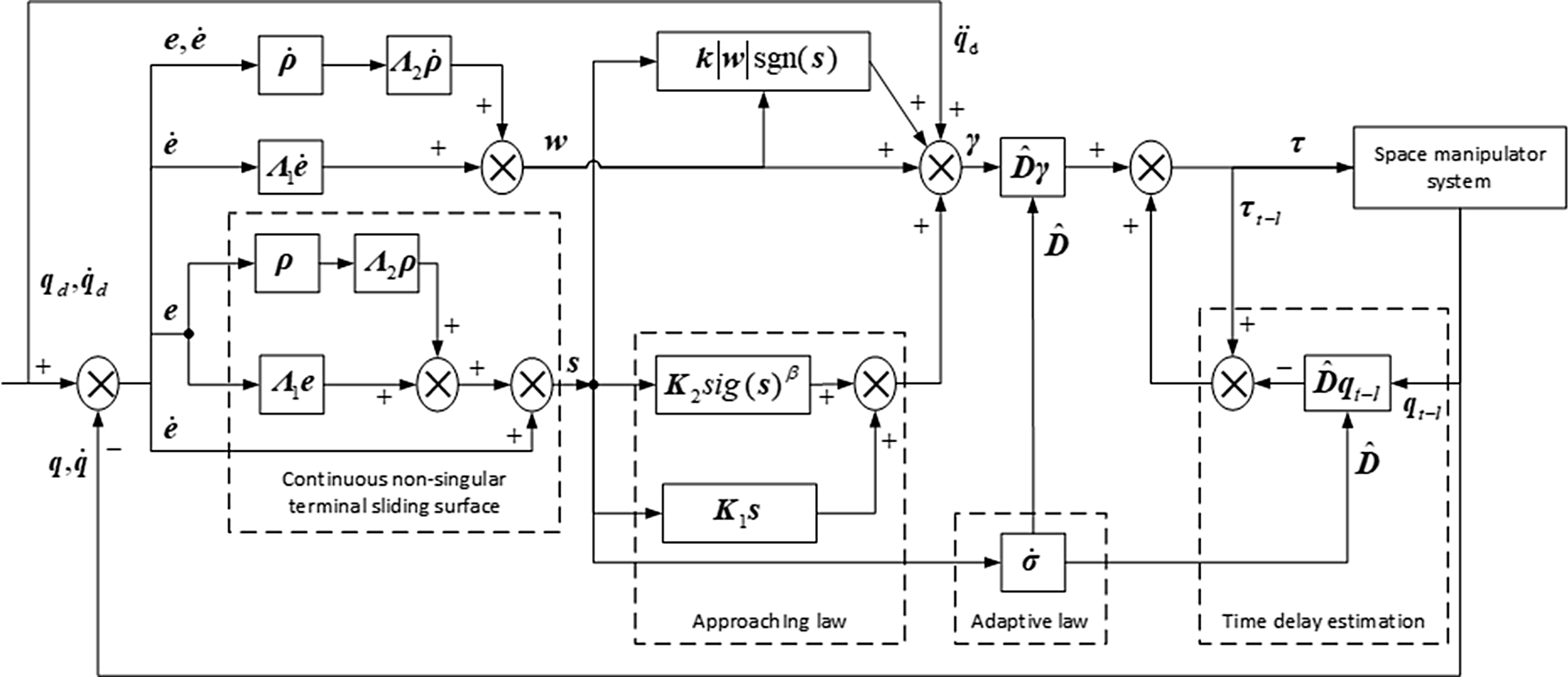
The operational control strategy of the proposed TDE-based adaptive sliding mode controller (42) is shown in Fig. 3.

Figure 3.

The operational control strategy of the TDE-based adaptive sliding mode controller.

5. Simulation examples

Simulations are carried out for a free-floating three-bar space manipulator, as shown in Fig. 1. The system’s parameters are as follows: ${m_0} = 1430{\mathop{\rm kg}\nolimits} $ , ${m_1} = 35{\mathop{\rm kg}\nolimits} $ , ${m_2} = 22.5{\mathop{\rm kg}\nolimits} $ , ${m_3} = 21.9{\mathop{\rm kg}\nolimits} $ , ${J_0} = 7090{\mathop{\rm kg}\nolimits} {\cdot} {{\mathop{\rm m}\nolimits} ^2}$ , ${J_1} = 0.42{\mathop{\rm kg}\nolimits} {\cdot} {{\mathop{\rm m}\nolimits} ^2}$ , ${J_2} = 0.94{\mathop{\rm kg}\nolimits} {\cdot} {{\mathop{\rm m}\nolimits} ^2}$ , ${J_3} = 0.63{\mathop{\rm kg}\nolimits} {\cdot} {{\mathop{\rm m}\nolimits} ^2}$ , ${l_0} = 0.5{\mathop{\rm m}\nolimits} $ , ${l_{\rm{1}}} = {\rm{0}}{\rm{.35}}{\mathop{\rm m}\nolimits} $ , ${l_2} = 0.87{\mathop{\rm m}\nolimits} $ , ${l_3} = 0.63{\mathop{\rm m}\nolimits} $ , ${b_{\rm{1}}} = 0.25{\mathop{\rm m}\nolimits} $ , ${b_2} = 0.175{\mathop{\rm m}\nolimits} $ , ${b_3} = 0.315{\mathop{\rm m}\nolimits} $ , $v = 1.2{\rm{m/s}}$ , ${\theta _0} = - \dfrac{\pi}{6}rad$ , $d = {\rm{2}}{\rm{.3}}{\mathop{\rm m}\nolimits} $ , ${\theta _p} = 242^\circ $ , ${\dot x_P} = 0.95{\mathop{\rm m}\nolimits} /s$ , ${\dot y_P} = - 0.55{\mathop{\rm m}\nolimits} /s$ , ${\dot \theta _p} = 0.13{\rm{rad/s}}$ , $[{({{{\ddot{\textbf{q}}}}_l})_{int}}] = {[{0.05}\quad {}{0.05} \quad {}{0.05} ]^{\textrm{T}}}$ $(^\circ {\rm{/}}{s^2})$ .

Assume $L = 0.01{\mathop{\rm s}\nolimits} $ , ${t_0} = 0s$ , ${t_f} = 66s$ , $[\Delta v] = 0.02{\rm{m/s}}$ , $\xi (0) = {[0.03\;\;0.02\;\;0.02]^{\textrm{T}}}$ . The controller parameters are ${{\textbf{D}}_I} = {\mathop{\rm diag}\nolimits} \left( {1,1,1,0.4,0.3,0.1} \right)$ , ${{\boldsymbol{\Lambda }}_{\rm{1}}} = {{\boldsymbol{\Lambda }}_{\rm{2}}} = {\mathop{\rm diag}\nolimits} \left( {30,30,30,30,30,30} \right)$ , ${{\textbf{K}}_{\rm{1}}} = {\mathop{\rm diag}\nolimits} \left( {2,2,2.4,2,2,2.4} \right)$ , ${{\textbf{K}}_{\rm{2}}} = {\mathop{\rm diag}\nolimits} ({\rm{0}}{\rm{.012}},0.0{\rm{12}},{\rm{2}}{\rm{.4}},{\rm{0}}{\rm{.012}},0.0{\rm{12}},{\rm{2}}{\rm{.4}})$ , ${{\alpha }_{1i}} = 0.8$ , ${{\alpha }_{2i}} = 1.4$ , ${{\alpha }_{3i}} = 2$ , ${\phi _i} = 0.002$ , ${k_{1i}} = 0.23$ , ${k_{2i}} = 0.2$ , ${{\zeta }_{1i}} = 0.5$ , ${{\upsilon }_i} = 0.1$ , ${\chi _i} = 0.1$ , $\beta = 0.{\rm{9}}$ , $i = 1, \cdots ,6$ .

Case 1 $\psi = - \dfrac{\pi}{6}rad$ , $\phi = \dfrac{\pi}{3}$ , the initial position of the base centroid relative to center of the target is $x_{C0}^P = - 7.67m$ , $y_{C0}^P = 1.77m$ .

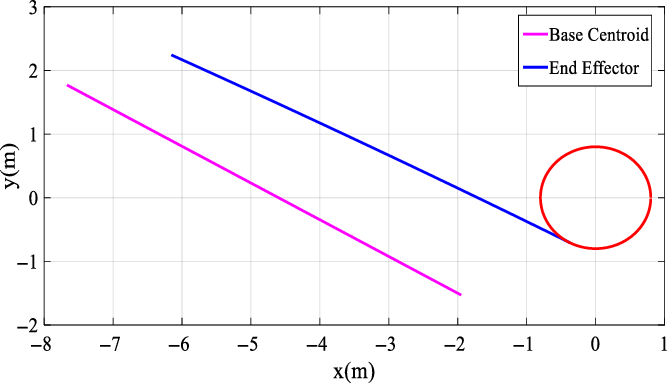
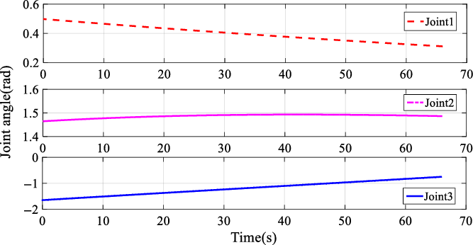
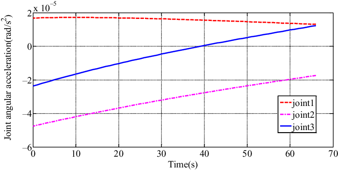
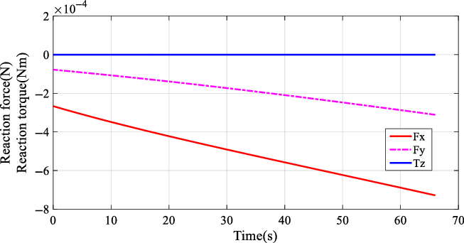
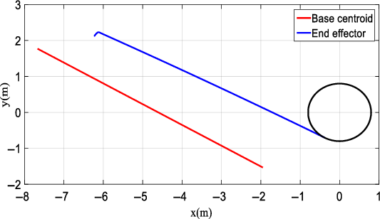
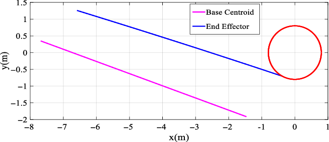
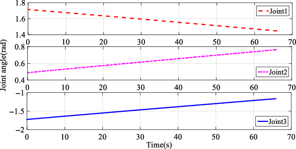
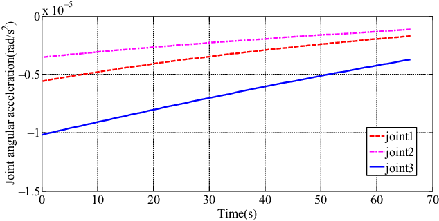
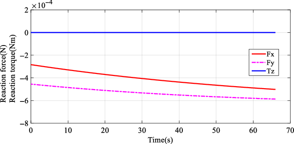
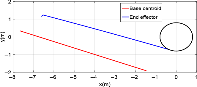
The simulation results of the RNS planning are shown in Figs. 4–7. Figure 4 shows the reactionless trajectories of the base centroid, the center of the end gripper. Figure 5 shows the reactionless joint trajectories, while Fig. 6 shows the reactionless joint angular accelerations. Figure 7 shows the reaction forces and reaction torque on the base.

Figure 4.

The reactionless trajectories of the base centroid, the center of the end gripper (RNS planning, $\psi = - \dfrac{\pi}{6}rad$ ).

Figure 5.

The reactionless joint trajectories (RNS planning, $\psi = - \dfrac{\pi}{6}rad$ ).

Figure 6.

The reactionless joint angular accelerations (RNS planning, $\psi = - \dfrac{\pi}{6}rad$ ).

Figure 7.

The reaction forces (RNS planning, $\psi = - \dfrac{\pi}{6}rad$ ).

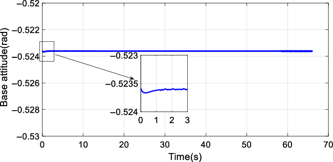
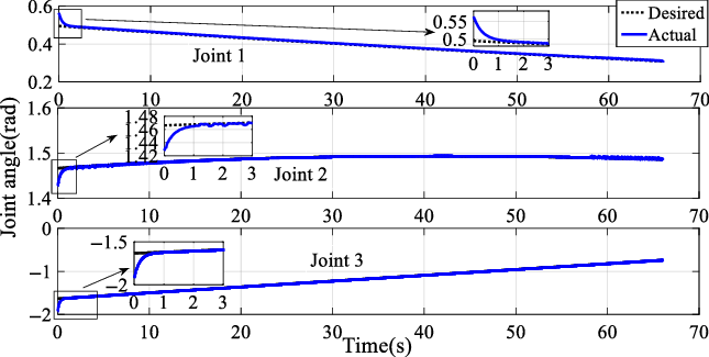
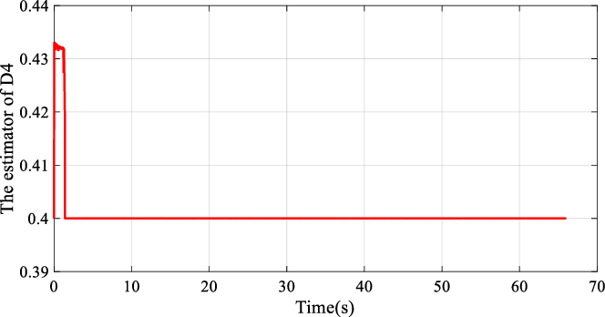
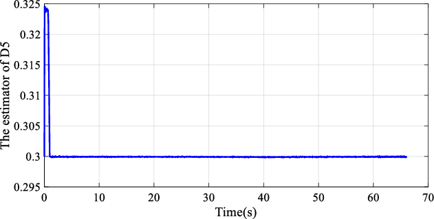
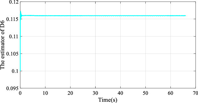
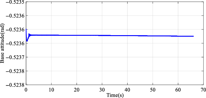
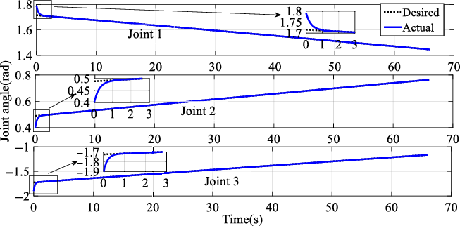
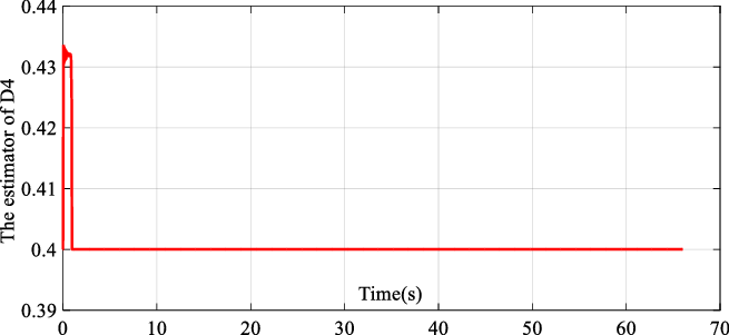
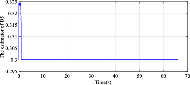
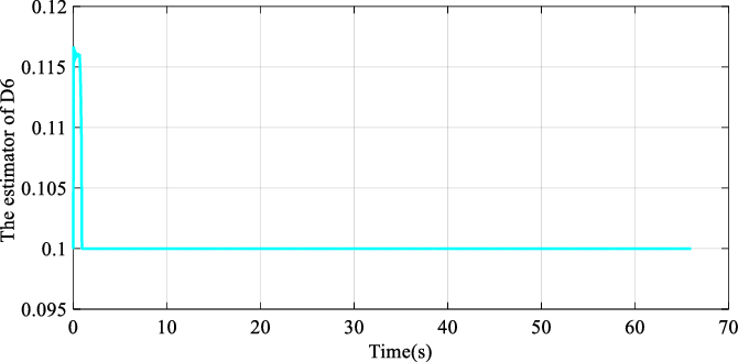
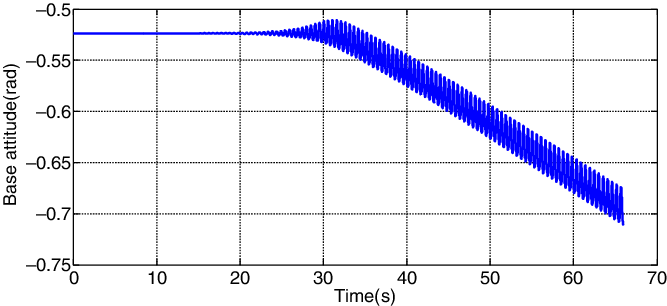
The initial state is ${\theta _1} = 0.56rad$ , ${\theta _2} = 1.43rad$ , ${\theta _3} = - 1.92rad$ , and the simulation results from the proposed controller Eq. (47) (controller II) are shown in Figs. 8–13. Figure 8 shows the actual trajectories of the base centroid, the center of the end gripper. Figure 9 is the actual trajectory of the base’s attitude, while Fig. 10 depicts the tracking trajectories of joints. Figures 11, 12, and 13 are the estimators of ${{D}_4}$ , ${{D}_5}$ , and ${{D}_6}$ , respectively. When the end gripper comes into contact with the target handle, $\Delta v$ is ${\rm{0}}{\rm{.0064}}\,{\rm{m/s}}$ . 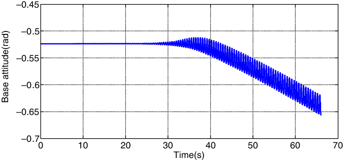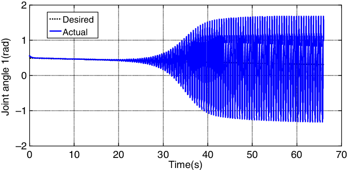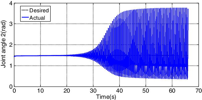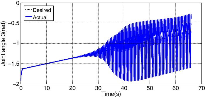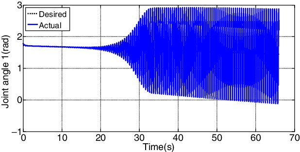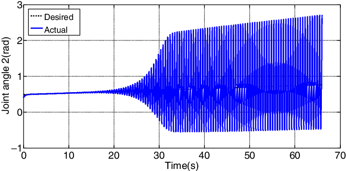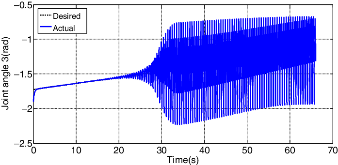The simulation results from the controller Eq. (33) (controller I) are shown in Figs. 14–17. Figure 14 is the actual trajectory of the base’s attitude, while Figs. 15–17 depict the tracking trajectories of joints 1–3, respectively.

Figure 8.

The actual trajectories of the base centroid, the center of the end gripper ( $\psi = - \dfrac{\pi}{6}rad$ , controller II).

Figure 9.

The tracking trajectory of the base’s attitude ( $\psi = - \dfrac{\pi}{6}rad$ , controller II).

Figure 10.

The tracking trajectory of joints ( $\psi = - \dfrac{\pi}{6}rad$ , controller II).

Figure 11.

The estimator of ${{D}_4}$ ( $\psi = - \dfrac{\pi}{6}rad$ , controller II).

Figure 12.

The estimator of ${{D}_5}$ ( $\psi = - \dfrac{\pi}{6}rad$ , controller II).

Figure 13.

The estimator of ${{D}_6}$ ( $\psi = - \dfrac{\pi}{6}rad$ , controller II).

Figure 14.

The tracking trajectory of the base’s attitude ( $\psi = - \dfrac{\pi}{6}rad$ , controller I).

Figure 15.

The tracking trajectory of joint 1 ( $\psi = - \dfrac{\pi}{6}rad$ , controller I).

Figure 16.

The tracking trajectory of joint 2 ( $\psi = - \dfrac{\pi}{6}rad$ , controller I).

Figure 17.

The tracking trajectory of joint 3 ( $\psi = - \dfrac{\pi}{6}rad$ , controller I).

Case 2 $\psi = - \dfrac{\pi}{9}rad$ , $\phi = \dfrac{\pi}{3}$ , the initial position of the base centroid relative to center of the target is $x_{C0}^P = - 7.67m$ , $y_{C0}^P = 0.34m$ .

The simulation results of the RNS planning are shown in Figs. 18–21. Figure 18 shows the reactionless trajectories of the base centroid, the center of the end gripper. Figure 19 shows the reactionless joint trajectories, while Fig. 20 shows the reactionless joint angular accelerations. Figure 21 shows the reaction forces and the reaction torque on the base.

Figure 18.

The reactionless trajectories of the base centroid, the center of the end gripper (RNS planning, $\psi = - \dfrac{\pi}{9}rad$ ).

Figure 19.

The reactionless joint trajectories (RNS planning, $\psi = - \dfrac{\pi}{9}rad$ ).

Figure 20.

The reactionless joint angular accelerations (RNS planning, $\psi = - \dfrac{\pi}{9}rad$ ).

Figure 21.

The reaction forces (RNS planning, $\psi = - \dfrac{\pi}{9}rad$ ).

The initial state is ${\theta _1} = 1.79rad$ , ${\theta _2} = 0.40rad$ , ${\theta _3} = - 1.90rad$ , and the simulation results from the proposed controller Eq. (47) (controller II) are shown in Figs. 22–27. Figure 22 shows the actual trajectories of the base centroid, the center of the end gripper. Figure 23 is the actual trajectory of the base’s attitude, while Fig. 24 depicts the tracking trajectories of joints. Figures 25, 26, and 27 are the estimators of ${{D}_4}$ , ${{D}_5}$ , and ${{D}_6}$ , respectively. When the end gripper comes into contact with the target handle, $\Delta v$ is ${\rm{0}}{\rm{.0192}}\,{\rm{m/s}}$ . The simulation results from the controller Eq. (33) (controller I) are shown in Figs. 28–31. Figure 28 is the actual trajectory of the base’s attitude, while Figs. 29–31 depict the tracking trajectories of joints 1–3, respectively.

Figure 22.

The actual trajectories of the base centroid, the center of the end gripper ( $\psi = - \dfrac{\pi}{9}rad$ , controller II).

Figure 23.

The tracking trajectory of the base’s attitude ( $\psi = - \dfrac{\pi}{9}rad$ , controller II).

Figure 24.

The tracking trajectories of joints ( $\psi = - \dfrac{\pi}{9}rad$ , controller II).

Figure 25.

The estimator of ${{D}_4}$ ( $\psi = - \dfrac{\pi}{9}rad$ , controller II).

Figure 26.

The estimator of ${{D}_5}$ ( $\psi = - \dfrac{\pi}{9}rad$ , controller II).

Figure 27.

The estimator of ${{D}_6}$ ( $\psi = - \dfrac{\pi}{9}rad$ , controller II).

Figure 28.

The tracking trajectory of the base’s attitude ( $\psi = - \dfrac{\pi}{9}rad$ , controller I).

Figure 29.

The tracking trajectory of joint 1 ( $\psi = - \dfrac{\pi}{9}rad$ , controller I).

Figures 6 and 20 show that the reactionless joint angular accelerations are less than their allowable values, and Figs. 7 and 21 show that the reaction forces and reaction torque on the base are almost 0. It can be seen from Figs. 9 and 23 that the base’s attitude changes slightly at the beginning, and then remains to be $ - \dfrac{\pi}{6}rad$ by the controller II. Meanwhile, it can be seen from Figs. 10 and 24 that the joint angles gradually track the desired reactionless trajectories and that the errors converge to zero after about 2 s by the controller II. From Figs. 14–17 and 28–31, it can be seen serious chattering happens after 20 s, and the reactionless desired joint trajectories cannot be tracked efficiently by the controller I .

Figure 30.

The tracking trajectory of joint 2 ( $\psi = - \dfrac{\pi}{9}rad$ , controller I).

Figure 31.

The tracking trajectory of joint 3 ( $\psi = - \dfrac{\pi}{9}rad$ , controller I).