





1 Introduction
In this article, we introduce a concept that interpolates between the classical ideas of braids and plats. Braids are of wide mathematical interest in fields including topology, group theory, contact geometry, and algebraic geometry – see the survey article [Reference Birman and BrendleBB05]. In particular, every link in
$S^3$
 can be encoded as a braid and thus understood via Artin’s braid group [Reference ArtinArt25]. Our proposed generalization of braids allows us, in principle, to reduce various topological questions from link theory to algebraic questions as in the braid case. It also allows us to extend the rich library of foliation-related techniques developed for braids to a larger class of links.
1.1 Book links
Let Y be an arbitrary three-manifold with a fixed open book decomposition, that is, a link
$B\subset Y$
 with a fibration
$p: (Y-B)\rightarrow S^1$
 with
$D_\theta $
 pages, equivalently, a circle-valued Morse function on
$Y-B$
 without critical points. A link L is an embedding
$\bigsqcup S^1\hookrightarrow Y-B$
 . The traditional definition of a closed braid is a link that intersects each page
$D_\theta $
 in the fibration transversely, equivalently, a link where
$p\circ L$
 is also a Morse function without critical points. We define a closed book link to be a link that intersects pages transversely except at finitely many non-degenerate critical points, equivalently, where
$p\circ L$
 is a Morse function. We will study book links up to book link isotopy – isotopies through book links, equivalently, through book links with the same number of critical points. We will generally suppress references to the three-manifold and open book decomposition and will assume that any link is embedded in a fixed three-manifold equipped with an open book decomposition and that any book link structure is the one induced by that open book decomposition. One can define a book link analog of an open braid as an appropriate non-degenerate tangle in a thickened surface, modulo isotopies rel boundary that fix the number of critical points.
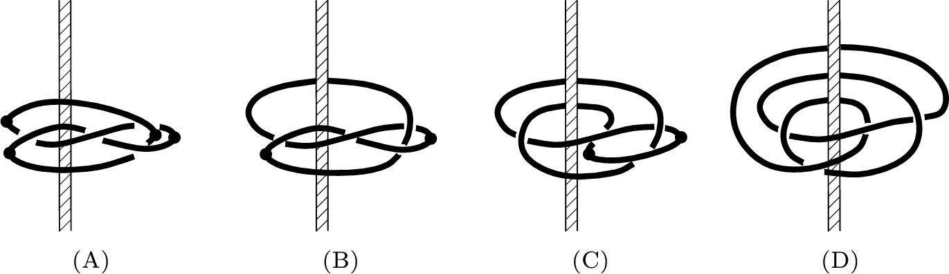
Each of these book link isotopy classes has a pair of invariants, the bridge index or number of critical points, and the braid index or minimum geometric intersection number with a page (minimized over the book link isotopy class). Just as a braid is a book link with bridge index zero, but potentially with high braid index, a plat closure can be viewed naturally as a book link that has arbitrarily high bridge index but braid index zero. The concept of a book link thus connects these two concepts. Figure 1 shows four different book link realizations of the same knot in
$S^3$
 with unknotted binding and various bridge and braid indices.
Book link realizations of the figure 8 knot which are (a) 2-bridge, 0-braid, (b) 1-bridge, 1-braid, (c) 1-bridge, 2-braid, and (d) 0-bridge, 3-braid. The solid dots indicate critical points while the binding is the vertical arc.

Figure 1 Long description
The diagram consists of four panels labeled A, B, C, and D from left to right. Each panel features a vertical hatched bar representing the binding and a thick black line representing the figure 8 knot. Solid black dots mark critical points on the knot.
* Panel A shows a 2-bridge, 0-braid realization. The knot is tightly clustered in front of the binding with two critical points on the far left and right edges.
* Panel B shows a 1-bridge, 1-braid realization. One arc of the knot extends further to the left of the binding, while the rest of the knot remains centered, with one critical point on the lower left, and another on the lower right.
* Panel C shows a 1-bridge, 2-braid realization. The knot forms is formed by two arcs that wrap around the binding, with a pair of critical points located in front of the binding.
* Panel D shows a 0-bridge, 3-braid realization. The knot wraps three times around the binding, without any critical points.
Throughout this article, the reader may find it helpful to take
$\mathbb {R}^3$
 with cylindrical coordinates as a prototypical example of a manifold equipped with an open book. Here, the z-axis is the binding of the open book and the pages
$H_\theta $
 are the points sharing the same angle
$\theta $
 . In this case, a braided knot is an embedding
$\textbf {r}: S^1 \hookrightarrow \mathbb {R}^3$
 that misses the z-axis with tangent vector transverse to
$H_\theta $
 , while a book knot is an embedding where, if the tangent vector is parallel to
$H_\theta $
 , then the normal vector is not. Equivalently, if
$\textbf {r} = (r,\theta ,z)$
 is parameterized using cylindrical coordinates, a braid obeys
$\theta '(t) \neq \text{0}$
 , while a book link has
$\theta $
 with only non-degenerate critical points, that is, if
$\theta '(t)=\text{0}$
 , then
$\theta "(t)\neq \text{0}$
 . The general case of a link in an open book decomposition of a three-manifold is locally identical.
While book links are natural objects of study in their own right, they have appeared recently in the context of Floer homology. For example, a key step in the proof of Baldwin–Sivek’s classification of genus one “nearly fibered” knots amounts to classifying bridge index one book links satisfying a simple topological condition [Reference Baldwin and SivekBS25, Section 6]. The second author used this result, along with similar results due to Birman–Menasco [Reference Birman and MenascoBM93] in the classical braid setting, to give various detection results for categorified link invariants [Reference BinnsBin25]. In related work, the second author and Dey classify links whose link Floer homology satisfies a simple algebraic condition; one case of their classification includes a family of bridge number one book links together with the bindings of the corresponding open books [Reference Binns and DeyBD24].
1.2 Classification results
Given that book links are a topological generalization of braids, we have the following natural question: To what extent do topological results concerning braids extend to book links? In this article, we address two fundamental instances of this question.
One foundational result in the study of braids is Alexander’s Theorem, that any link in any three-manifold can be isotoped to a braid [Reference AlexanderAle23, Reference SkoraSko92]. The analogous statement in the setting of book links is discussed in Section 2.
Theorem 1.1 (Alexander’s theorem for book links)
Let Y be a three-manifold equipped with an open book decomposition. Any link
$L\subset Y$
 can be isotoped to a book link
$\lambda $
 with any desired (even) number of critical points on each component.
This result can also be thought of as a generalization of the fact that every link can be put bridge position. Another foundational result in braid theory is Markov’s theorem, which characterizes when distinct braid representatives of a fixed link are isotopic [Reference BirmanBir74, Reference Márkov Már35 , Reference SkoraSko92]. The plat version of the Markov theorem was proven by Birman in [Reference BirmanBir76]. Our main goal in this article is to generalize Markov’s theorem to the book link setting. We say two book links are of the same critical point type if they are of the same link type and the corresponding components have the same number of critical points.
Theorem 1.2 (Markov’s theorem for book links)
Let Y be a three-manifold equipped with an open book decomposition. If
$\lambda _1$
 and
$\lambda _2$
 are book links in Y of the same critical point type, then they are related by a sequence of book link isotopies and stabilizations and destabilizations.
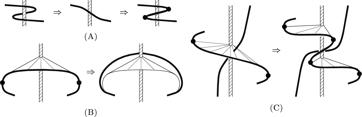
Observe that, if we allow not just braid stabilizations and destabilizations as shown in Figure 2a but also allow birth and canceling of critical points, that is, all the moves shown in Figure 2, then this theorem follows immediately from the traditional plat and braid Markov theorems (we must merely apply the figure moves to the booklinks until they are both pure braids/plats and then apply the traditional braid Markov theorems).
The book link structure and braid/bridge indices may be altered (a) by stabilization and destabilization through the braid axis or by a local perturbation; and (b) by an isotopy of a segment with a pair of critical points which has a free path to the braid axis. A segment without a free path may be modified as in (c).

Figure 2 Long description
The diagram consists of three panels labeled A, B, and C. Each panel features a vertical hatched rectangular bar representing a braid axis and thick black lines representing segments or strands.
* Panel A at the top left shows a three-step sequence. First, a strand loops around the axis. Second, the loop is removed, leaving a single diagonal strand crossing the axis. Third, two critical points marked by black dots are added to create a new zig-zag fold across the axis.
* Panel B at the bottom left shows a two-step isotopy. On the left, a curved strand with two critical point is connected to the axis by a fan-like bridge of thin lines. An arrow points to the right, where the strand has been pulled across the axis, removing the pair of critical points.
* Panel C on the right shows a complex modification of a segment without a free path to the axis. The left side shows a curved strand with one critical point and a large fan-like bridge structure connecting to the axis. The right side, following a double arrow, shows the strand broken into multiple segments with four critical points and two separate bridge structures along the vertical axis.
Here, the operations of stabilizations and destabilizations are defined exactly as in the braid case; in particular, they preserve the number of critical points. It follows directly from the theorem that any two book link representatives of the same link type – even if not the same book link type – can be connected via book link isotopies, stabilization/destabilization, and the creation/cancellation of critical points.
To prove this theorem, we extend the theory of braid foliations to surfaces with book link boundary. For braids, this machinery was first developed by Birman and Menasco in a sequence of papers [Reference Birman and MenascoBM05, Reference Birman and MenascoBM90, Reference Birman and MenascoBM91, Reference Birman and MenascoBM92a, Reference Birman and MenascoBM92b, Reference Birman and MenascoBM92c, Reference Birman and MenascoBM93]. The text of LaFountain and Menasco gives an excellent exposition on braids and foliation techniques which we adapt here [Reference LaFountain and MenascoLM17].
1.3 A spectrum of invariants
We discuss invariants of links derived from book links which encompass and unify the classical braid and bridge indices. Given that every link can be isotoped to a book link with any bridge index (Theorem 2), we can extract a spectrum of invariants from book links. More details appear in the paper of Doig and Gehringer [Reference Doig and GehringerDG], which shows the behavior of the spectrum for split and composite links and calculates the spectrum for prime knots through nine crossings.
Definition 1.1 The book index spectrum of a link L is the sequence
$\big \{b_L(d)\big \}_{d=0}^\infty $
 , where
$b_L(d)$
 is the minimum braid index of a book link representative of L with bridge index d.
For a link L in
$S^3$
 with the standard open book decomposition, the quantity
$b_L(\text{0})$
 recovers the classical definition of the braid index of L, that is, the minimum braid index over all braid representatives of the link. Similarly, the first d for which
$b_L(d)=\text{0}$
 is exactly the classical bridge index of L. Observe that if L has a book link representative of braid index n and bridge index d then L admits a book link representative with braid index n and bridge index
$d+\text{1}$
 that can be obtained by perturbing a segment of L without critical points to introduce a pair of canceling critical points. It follows that
$b_L:{\mathbb {Z}}^{\geq 0}\to {\mathbb {Z}}^{\geq 0}$
 is a non-increasing function.
One can show that the function
$b_L$
 is strictly decreasing between
$\text{0}$
 and the bridge index of L. It follows that torus links and other BB-links (those with the same classical bridge and braid index, say n) satisfy
$b_L(d)=n-d$
 for
$\text{0} \leq d \leq n$
 and
$b_L(d)=\text{0}$
 else. For an unknot U,
$b_U(\text{0})=\text{1}$
 and
$b_U(k)=\text{0}$
 for
$k> \text{0}$
 .
For a fixed link L, a book link representative of L may be substantially “simpler” than the simplest braid representative of L in the sense that
$b_L(d)$
 may be arbitrarily larger than
$b_L(d+\text{1})$
 . For example, Schubert’s classification of 2-bridge knots includes knots with arbitrarily high braid index [Reference SchubertSch56], that is, with
$b_{L_n}(\text{0})=n$
 ,
$b_{L_n}(\text{1})=\text{1}$
 , and
$b_{L_n}(i)=\text{0}$
 for
$i\geq \text{2}$
 . By adding split unlinked components to
$L_n$
 , it can be shown that there are links L for which
$b_L(d)-b_L(d+\text{1})$
 is arbitrarily large for any fixed d.
The book index spectrum resembles the bridge spectrum of a knot introduced by Zupan to capture bridge indices of knots with respect to higher genus Heegaard surfaces of
$S^\text{3}$
 [Reference ZupanZup14].
1.4 Questions
We end this section with some questions. First, recall that braids admit equivalent characterizations via mapping class groups or configuration spaces [Reference ArtinArt25, Reference BirmanBir74].
Do book links admit interpretations analogous to the mapping class or configuration space interpretations of braids?
Book links can be thought of as “closures” of tangles in thickened surfaces with the same number of critical points of index 0 and 1. With this in mind, one might relate such tangles to objects of a more algebraic flavor by appealing to an appropriately modified “tangle category” (see [Reference TuraevTur89, Section 3]). For example, in [Reference TuraevTur89, Theorem 3.2], one could remove the relations corresponding to (a), (b), (c), and (f) in [Reference TuraevTur89, Figure 4]. To move from an algebraic classification of such tangles to an algebraic classification of book link closures would require a slightly more subtle analysis than in the braid case, to account for isotopies which push the critical points of the book link through, for instance, every page of the open book.
Next is the problem of distinguishing book links up to book link isotopy. Given a book link
$\lambda $
 one can form the link
$\lambda \cup B$
 where B is the axis of
$\lambda $
 . Any classical link invariant of
$\lambda \cup B$
 is a book link isotopy invariant of
$\lambda $
 . This implies, for instance, that the annular Whitehead link and its mirror –
$T_0$
 and
$T_{-1}$
 – can be distinguished via the signature of
$T_i\cup B$
 .
What are the book link isotopy classes of the unknot with fixed braid and bridge indices?
Baldwin–Sivek implicitly gave a partial result in this direction, classifying specific types of braid index
$\text{3}$
 representatives of the unknot [Reference Baldwin and SivekBS25, Proof of Theorem 6.1]. They use this to prove various knot detection results for knot Floer homology and Khovanov homology. One might hope to obtain further link detection results by giving similar book link classifications.
We may also ask how difficult it is to distinguish book link isotopy classes.
What is the computational complexity of determining whether two book links are book link isotopic?
For example, Hass, Lagaris, and Pippenger demonstrated the first result along these lines by showing that distinguishing a PL link from the unlink is in NP, as is identifying a link as split [Reference Hass, Lagarias and PippengerHLP99].
Open book foliations have a number of important topological applications.
Can the techniques of open book foliations be extended to study surfaces in book link complements?
For example, open book foliations can be used to prove the Bennequin–Eliashberg inequality [Reference Ito and KawamuroIK14a, Theorem 4.3] and the Jones conjecture [Reference LaFountain and MenascoLM14], to define practical invariants such as self-linking number for transverse knots, and to relate the geometry of certain three-manifolds to the fractional Dehn twist coefficients of their possible open book structures [Reference Ito and KawamuroIK17, Theorem 8.3]. We note that there has also been some recent work adapting aspects of braid foliation theory to the setting of plat closures [Reference Menasco and SolankiMS24, Reference SolankiSol23], which suggests possible success in extending these techniques to the overarching book link case.
Similarly, it may be enlightening to extend other braid techniques to book links.
Do any braid invariants – for example, the self-linking number – have book link analogs?
Finally, given Theorem 1.2, we have the following natural question.
Fix
$k\geq \text{0}$
 . For each
$n\in {\mathbb {Z}}$
 , do there exist braid index n book links which are only book link isotopic after exactly k stabilizations?
Outline
In Section 2, we prove a stronger version of Theorem 1.1, Alexander’s theorem for book links. In Section 3, we consider an embedded surface bounded by a book link and study the foliation induced upon it by the open book decomposition of the manifold. In Section 4, we prove Theorem 1.2 using the open book foliations of embedded annuli bounded by book links.
2 An Alexander theorem for book links
The concept of a book link is generic enough to have a version of Alexander’s theorem which allows us to convert any link into a book link with the desired number of critical points. Theorem 1.1 in the introduction is a particular case (
$\beta =\emptyset $
 ) of the following result.
Alexander’s theorem for book links Let Y be a three-manifold with a fixed open book decomposition and
$\beta $
 be a book link. Then, for any
$L\subset Y\setminus \beta $
 , the link
$L\cup \beta $
 can be isotoped to a book link
$\lambda \cup \beta $
 , where
$\lambda $
 has any desired (even) number of critical points on each component, and the isotopy restricted to
$\beta $
 is a book link isotopy.
Proof A local perturbation will resolve any degenerate critical point into 1 or 2 non-degenerate critical points, that is, we may immediately convert a link L into a book link
$\lambda $
 .
If
$\lambda $
 has too few critical points, it is easy to add additional ones, just as we may stabilize or destabilize in the traditional braid fashion (see Figure 2a). This operation may be realized by an isotopy which is the identity away from the replacement area.
If
$\lambda $
 has too many critical points, they may be resolved in pairs following an argument similar to that of Lemma 2.3 in [Reference LaFountain and MenascoLM17]. First, suppose there are two critical points connected by a segment with no other critical points as in Figure 2b. If there is a point on the braid axis and an interval family of continuously varying arcs, each lying in a single page, which connect the segment to that point, and if these paths are disjoint from the rest of
$\lambda \cup \beta $
 , then they will sweep out a triangle in the complement of
$\lambda \cup \beta $
 . We may isotope the segment through this triangle and push it to the other side of the braid axis; if we are careful, the intermediate segments will contain a matched pair of critical points until they converge in a single point when the segment intersects the braid axis. Then the intermediate segment passes through the braid axis and the critical points are eliminated.
If it is impossible to find such an interval family of arcs that do not intersect another segment of
$\lambda $
 or
$\beta $
 as in Figure 2c, we may locally alter both segments to remove the issue. This will introduce a new pair of critical points, but the four points may now be pairwise resolved – unless there is another intersecting segment to accommodate likewise, but this process will terminate in a finite number of steps.
We next consider how an isotopy between two links may be reflected as a sequence of book links connected by unions of annuli. This an extension of Proposition 2.8 of [Reference LaFountain and MenascoLM17] to book links and follows immediately by applying to the proposition Theorem 2, but we include a proof here for thoroughness.
Lemma 2.1 Suppose that
$\lambda _-$
 and
$\lambda _+$
 are book link representatives of a link in an arbitrary three-manifold. There is a finite collection of pairwise disjoint book links
$\lambda _-=\lambda _0$
 ,
$\lambda _1$
 , …,
$\lambda _m=\lambda _+$
 such that for each
$i=\text{1},\dots m$
 , there is a disjoint union of annuli
$A_i$
 with
$\partial _-A_i = \lambda _{i-1}$
 and
$\partial _+A_i = \lambda _i$
 . Furthermore, the braids
$\lambda _1, \dots , \lambda _{m-1}$
 can be chosen to be book links of the same critical point type.
Proof Observe that there exist piecewise linear links
$L_-$
 and
$L_+$
 such that
$\lambda _-$
 and
$\lambda _+$
 cobound families of embedded annuli with
$L_-$
 and
$L_+$
 , respectively. Pick a triangulation of Y so that
$L_-$
 and
$L_+$
 lie in the 1-skeleton. After a finite number of subdivisions, the
$L_-$
 and
$L_+$
 are related by a sequence of
$\Delta $
 -moves. Here, a
$\Delta $
 -move corresponds to taking an embedded triangle with one edge on L and replacing the arc on L with the two remaining edges of the triangle. We can subdivide the triangulation to ensure that no successive pairs of triangles intersect. Notice that each
$\Delta $
 -move traces a region that can be widened to an embedded annulus.
The sequence of
$\Delta $
 -moves can be used to build a family of n-tuples of oriented embedded annuli
$\{A_i\}_{i=1}^m$
 overlapping at their boundaries in links denoted by
$\lambda _i$
 , and, in fact, they do not intersect in their interiors, that is,
$\partial _-A_i = \lambda _{i-1}$
 and
$\partial _+A_i=\lambda _i$
 , as well as
$A_i \cap A_{i+1} = \lambda _i$
 . Theorem 2 guarantees the existence of an isotopy that converts each intermediate
$\lambda _i$
 into a book link with the appropriate number of critical points. This isotopy can be extended to an ambient isotopy, and the images of the unions of annuli under this isotopy are the desired
$A_i$
 .
3 Foliations, singularities, and tiles
To understand surfaces bounded by book links, as well as to prepare for the proof of Theorem 1.2, we study foliations induced by the pages of the open book decomposition of the manifold. In particular, we investigate the resulting singularities and their foliated neighborhoods.
We first expand Ito and Kawamuro’s definition of an open book foliation [Reference Ito and KawamuroIK14a] to accommodate surfaces bounded by book links and allow extremal singularities on the boundary only.
Definition 3.1 Consider a surface
$\Sigma $
 in a three-manifold Y equipped with an open book decomposition
$(B,p)$
 . Say
$\partial \Sigma = \lambda $
 is a book link and
$\mathcal {F}(\Sigma )$
 is the foliation on
$\Sigma $
 induced by the open book decomposition. We call
$\mathcal {F}(\Sigma )$
 an open book foliation if the following conditions hold:
$\Sigma $
 is pierced by the binding in finitely many points, at each of which the foliation is radial; all but finitely many pages are transverse to
$\Sigma $
 , and each exceptional page is tangent at a single point; and all tangencies are either extremal on
$\partial \Sigma $
 or of saddle type in
$\text {int}\Sigma $
 .
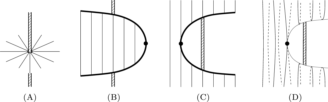
We call a component of the intersection of the surface with a single page a leaf, and it is either singular or regular. An elliptic point is an intersection point of the surface and the binding, as in Figure 3a. An extremal singularity is a point where the boundary is tangent to a page (equivalently, a local maximum or minimum with respect to the Morse function), as in Figure 3b and 3c. A hyperbolic singularity is a saddle point on the surface (equivalently, an index 1 critical point with respect to the Morse function), as in Figure 3d. Note that elliptic and hyperbolic singularities may be given signs based on whether the orientation of the surface agrees with the orientation of the binding or the pages, respectively.
(a) An elliptic point where the binding meets the surface, (b and c) extremal singularities on the boundary, and (d) a hyperbolic singularity in the interior of an open book foliation.

Figure 3 Long description
The diagram consists of four panels labeled A through D.
* Panel A shows an elliptic point. A vertical hatched bar representing the binding is interrupted by a small circle. From this central circle, straight lines radiate outward in all directions like spokes on a wheel.
* Panel B depicts an extremal singularity on a boundary. A thick parabolic curve opens to the left. A black dot is positioned at the vertex on the far right. Vertical lines fill the interior of the parabola, and the curve is intersected by a vertical hatched bar at the top and bottom.
* Panel C shows another extremal singularity. A thick parabolic curve opens to the right with a black dot at its vertex on the far left. Vertical lines pass through the entire frame, and a vertical hatched bar is positioned inside the curve's opening.
* Panel D illustrates a hyperbolic singularity in the interior. A black dot sits at the center of a saddle-like structure. To the left of the dot, vertical lines curve slightly away from the center. To the right, a thin parabolic boundary contains a vertical hatched bar. Dashed lines form loops that converge toward the central dot from the top and bottom, creating a cross-like flow pattern.
An open book foliation can have three types of leaf: arcs with both endpoints on B; arcs with an endpoint on
$\partial \Sigma $
 and an endpoint on B; and arcs with both endpoints on
$\partial \Sigma $
 .
Lemma 3.1 A surface with boundary a book link may be isotoped without changing the boundary to admit an open book foliation.
Proof We perturb the surface in such a manner that no two hyperbolic singularities occur on the same page. We may further assume that saddle points occur in the interior, or else we may move them into the interior by a small perturbation.
The work in [Reference Ito and KawamuroIK14a, Theorem 2.5] allows the removal of simple closed curves and interior extremal critical points in the case of a surface bounded by a braid. The same arguments apply in our setting because they only require a modification of the interior of the surface and not its boundary.
For the remainder of this article, we fix an arbitrary three-manifold, Y, equipped with an arbitrary open book decomposition
$(B,p)$
 . We assume that any surface
$\Sigma $
 we refer to is embedded in Y and equipped with the open book foliation induced by
$(B,p)$
 .
Next, we examine how singularities of an open book foliation lie with respect to one another in the surface and decompose the surface into a set of tiles following the work of [Reference Birman and MenascoBM92a, p. 30] for braids in
$S^3$
 and [Reference Ito and KawamuroIK14a, Section 2.1.3] for braids in an arbitrary
$Y^3$
 (see also the account in [Reference LaFountain and MenascoLM17, Lemma 2.4]. Recall each arc contains at most one hyperbolic or extremal singularity because an arc comes from an intersection of a page with the surface, and we have assumed that these singularities occur on discrete pages. The singular leaves are separated from one another by product foliations, in other words, the surface can be divided along non-singular leaves into a finite set of regions which are neighborhoods of singular leaves. We will commonly visualize these regions by flattening the surface and drawing lines to represent the foliation, which we show in Figure 4.
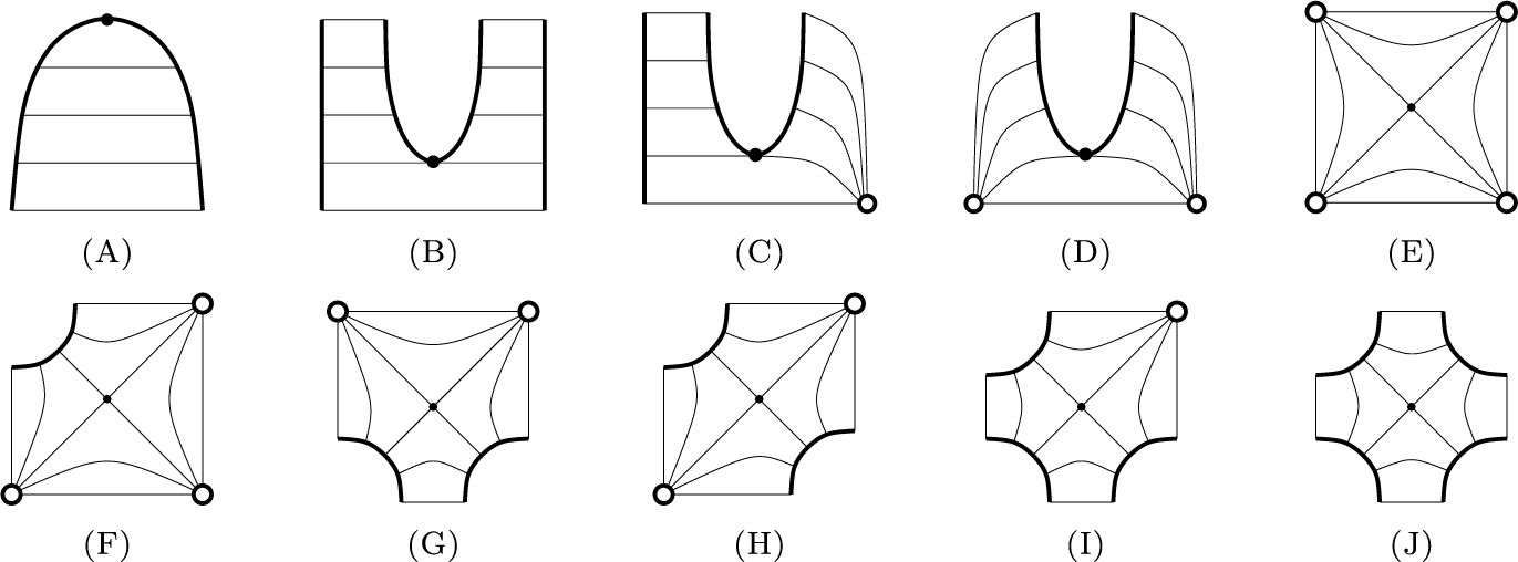
Definition 3.2 A tile is the neighborhood of a singular leaf. The tile in Figure 4a is called a
$\partial $
 -tile and the tile in Figure 4k is called an h-tile (in the language of [Reference LaFountain and MenascoLM17], a
$\partial $
 -tile is unnamed, and an h-tile is an
$ss$
 -tile).
Tiles for boundary extremal and hyperbolic interior singularities (solid dots), which are connected by singular leaves to either boundary segments (dark lines) or elliptic points (open dots). Lemma 3.2 explains how to eliminate tiles (b)–(d) by local perturbations and tiles (f), (g), (i) by stabilizations. Lemma 3.3 classifies the surfaces tiled by only the remaining tiles: a surface without boundary by (e); a surface bounded by a braid by (h); a surface bounded by a non-braid book link by (j) and (a) together (the h- and
$\partial $
 -tiles).

Figure 4 Long description
The diagram consists of two rows of five panels each, labeled A through J. Each panel depicts a square or rectangular tile containing singular leaves, solid dots representing singularities, and open dots representing elliptic points.
Top Row:
* Panel A: A dome-shaped boundary with a solid dot at the apex and horizontal singular leaves.
* Panel B: A U-shaped boundary with a solid dot at the base and horizontal singular leaves.
* Panel C: Similar to B, but the right side connects to an open dot at the bottom right corner.
* Panel D: Similar to C, but the left side connects to an open dot at the bottom left corner.
* Panel E: A square tile with a central solid dot and four open dots at the corners, connected by diagonal and curved singular leaves.
Bottom Row:
* Panel F: A square tile with one concave boundary segment at the top-left, a central solid dot, and three open dots at the remaining corners.
* Panel G: A square tile with two concave boundary segments at the bottom, a central solid dot, and two open dots at the top corners.
* Panel H: A square tile with two concave boundary segments at the top-left and bottom-right, a central solid dot, and two open dots at the top-right and bottom-left corners.
* Panel I: A square tile with three concave boundary segments and one open dot at the top-right corner, with a central solid dot.
* Panel J: A square tile with four concave boundary segments and a central solid dot, with no open dots.
Lemma 3.2 A surface with an open book foliation is (possibly after book link isotopies and stabilizations or destabilizations) either closed; a disk; a surface with braided boundary; or a surface with book link boundary which may be decomposed along non-singular leaves into a finite set of
$\partial $
 -tiles and h-tiles.
Proof The work in [Reference LaFountain and MenascoLM17, Lemma 2.4] ensures that the surface has a finite decomposition into tiles; however, the introduction of extremal singularities along the boundary allows additional tile types beyond those demonstrated by braids.
As in the case that the boundary is braided, we may assume each elliptic point is connected by an arc to at least one hyperbolic singularity, else there is a disk or sphere component. We may also assume that each hyperbolic singularity falls on a singular leaf whose four endpoints fall either at elliptic points or on the boundary since we may perturb the surface so that no two critical points occur in the same page. Therefore, the singularities of Figure 3 give rise to two possible extremal tiles and six possible hyperbolic tiles, whether the singular leaves end at elliptic points or on the boundary(see Figure 4). Note that there are strictly more possibilities here than in the case the boundary of the surface is assumed to be braided.
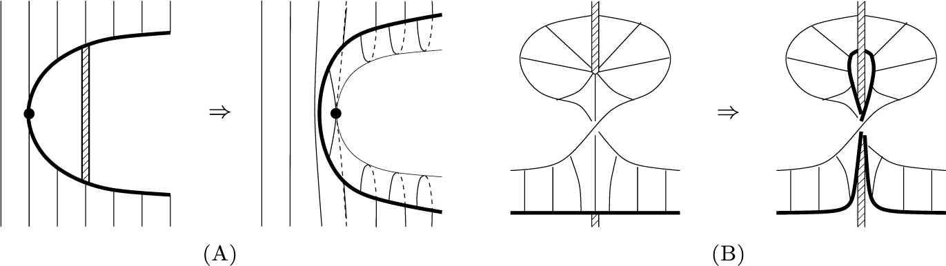
Figure 5 shows us how to remove some of these tiles. We may first perform a local perturbation on the interior of the surface to convert one type of boundary singularity into the other by adding a hyperbolic singularity, and so we may remove any instance of Figure 4b, 4c, or 4d, that is, any extremal singularity lies in a
$\partial $
 -tile. We may also stabilize the book link to remove a hyperbolic singularity and an elliptic point together à la [Reference LaFountain and MenascoLM17, Figure 2.22]. Thus, we may assume there are no tiles (Figure 4f, 4g, and 4i).
(a) A local perturbation eliminating one type of extremal singularity. (b) A stabilization eliminating an elliptic point and a hyperbolic singularity.

Figure 5 Long description
Panel A shows a transformation of a parabolic curve within a field of vertical lines. On the left, a thick black curve contains a single black dot at its leftmost vertex and a vertical hatched bar spanning its interior. A double-lined arrow points to the right, where the curve has been perturbed. The black dot remains, but the interior hatched bar is gone, replaced by dashed lines and small elliptical loops along the inner boundary of the curve. Panel B illustrates a stabilization process. On the left, a complex structure features a vertical hatched bar passing through a circular field with radiating lines that pinch at a central hyperbolic point. A double-lined arrow points to the right, showing the elimination of the singularity. The circular field has split into two distinct lobes, one above and one below a central gap, with the thick black boundary lines curving away from the vertical hatched bar to create a smooth, non-singular transition.
Once we have removed these tiles, if there is any tile remaining with four elliptic points as in Figure 4e, then the entire surface consists of only these tiles and so is closed. If there is a tile (Figure 4h), then, again, the entire surface must be tiled with the same tile, so the boundary will have no critical points and will be braided. Finally, h-tiles from Figure 4j can be glued to one another and to
$\partial $
 -tiles, giving a component of the surface with book link boundary.
We introduce one more tool to visualize the surface, in particular, to study how the singularities are connected to one another and the boundary. Represent a surface
$\Sigma $
 by a graph
$\Gamma (\Sigma )$
 : assign a vertex for each singularity and connect two vertices with an edge if their tiles are adjacent. In the special case where
$\Sigma $
 has only
$\partial $
 - and h-tiles, there will be a vertex of degree
$\text{4}$
 at each hyperbolic singularity and a vertex of degree
$\text{1}$
 at each extremal singularity. Additionally, if
$\Sigma $
 is an annulus with two boundary components, then the graph has a single simple cycle that divides the surface into two regions. If each boundary component is a book link of bridge index d, then each region has exactly
$\text{2}d$
 degree-1 vertices.
Finally, we will find it useful to isotope the surface in an appropriate neighborhood of a pair of hyperbolic singularities and examine how this isotopy is reflected in the transformation of the tiles and their graph. Similar techniques have previously been employed to study open book foliations, for example, in [Reference Birman and MenascoBM90, Figure 8] and [Reference Ito and KawamuroIK14b, Theorem 3.1].
Lemma 3.3 Let
$\Sigma $
 be a surface with an open book foliation and two adjacent h-tiles. Suppose that the edge between these tiles splits off a disk D from
$\Sigma $
 . Then there is an isotopy of
$\Sigma $
 , supported on a neighborhood of D, that restricts to a book link isotopy on the boundary, and which alters the foliation in a neighborhood of the two adjacent h-tiles as in Figure 6 and changes its graph
$\Gamma (\Sigma )$
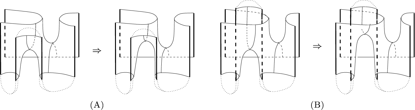
 as in Figure 7.
(a) Two isotopic surfaces used in Lemma 3.3 containing two h-tiles with the same orientation. The dotted lines represent topological disks formed from a tree consisting of h-tiles and
$\partial $
 -tiles. (b) The same for two h-tiles with opposite orientation.

Figure 6 Long description
The diagram consists of two panels labeled A and B arranged horizontally.
Panel A shows a continuous, undulating surface resembling a series of connected cylinders or tubes. Within this surface, two h-tiles are depicted with the same orientation. These tiles are represented by bold vertical lines and curves. Dotted lines trace topological disks that form a tree structure connecting the h-tiles and partial J tiles. A double-lined arrow points from the first set of tiles to a second configuration to the right where the heights of the saddles have been exchanged, indicating a transformation or relationship within the lemma.
Panel B displays a similar undulating surface. In this panel, the two h-tiles are shown with opposite orientations, where the bold vertical lines and curves are mirrored or inverted relative to each other. Like panel A, dotted lines represent the topological disks and tree structures. A double-lined arrow again points from the left configuration to the right configuration within the surface structure, where the heights of the saddles have been exchanged.
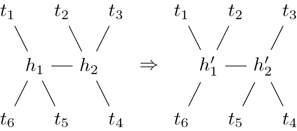
Graphs for the two isotopic surfaces of Figure 6. The subgraphs
$t_1$
 ,
$t_5$
 , and
$t_6$
 correspond to the dotted topological disks and so are trees (as is at least one of the other
$t_i$
 since the surface is an annulus).

Variations of this lemma are true for different conditions on the surface. This version depends heavily upon the fact that the edge between the tiles cuts off a topological disk from the rest of
$\Sigma $
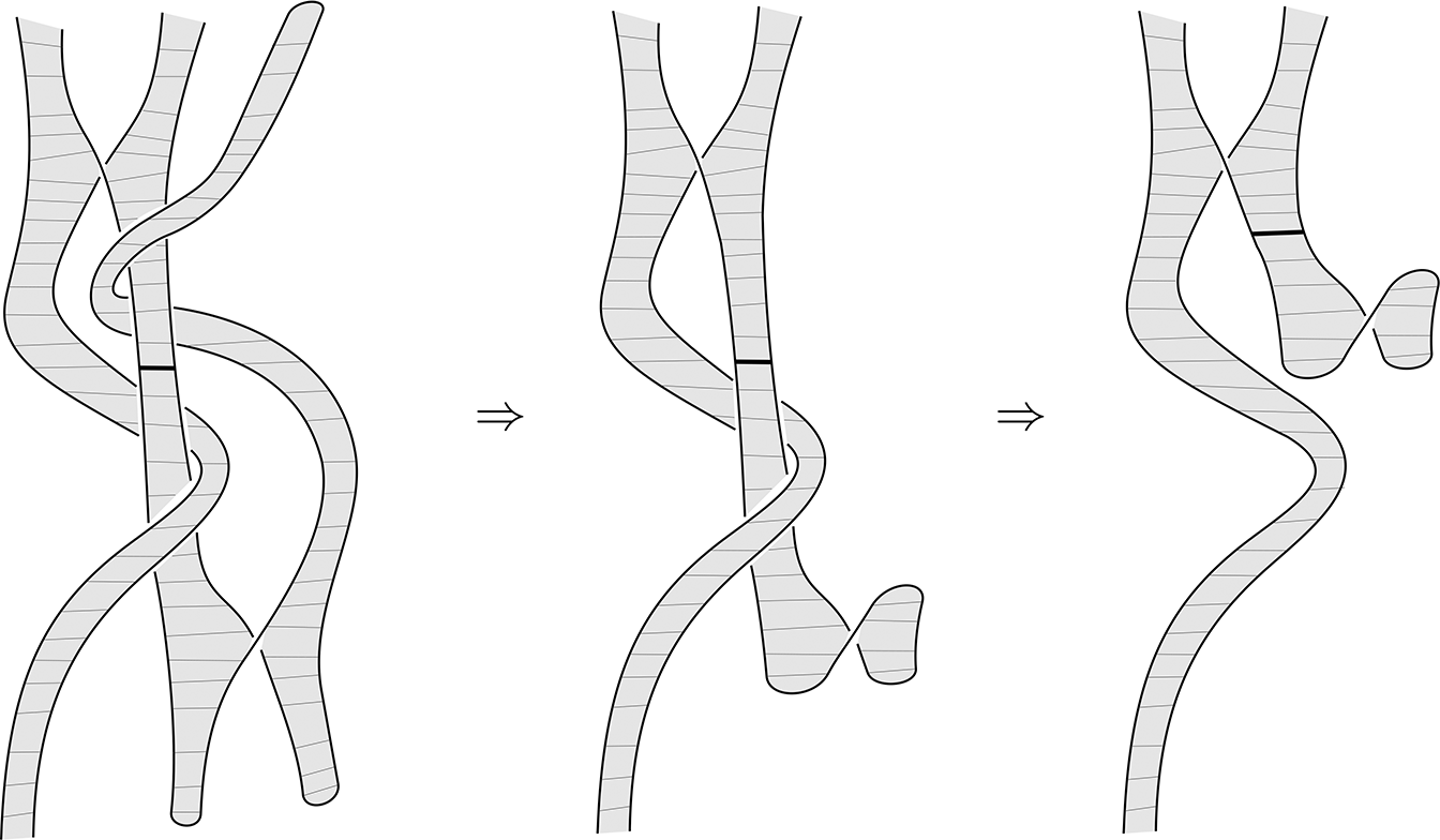
 . We emphasize that we are only modifying the surface and its foliation in a neighborhood of this pair of h-tiles and the disk D, not for any other portion of the surface. The first step in the proof will be to contract the disk so that the rest of the surface will not interfere with the isotopy. See Figure 8: despite the fact that one h-tile is capped off with three
$\partial $
 -tiles, its embedding appears to be knotted with the rest of the surface. In the example shown in Figure 8, we will first contract the three
$\partial $
 -tiles, then isotope the h-tile so it does not knot with any other part of the surface. If this h-tile were not capped off by three disks, then this isotopy may have been impossible.
Proof First, we ensure that the surface looks like the leftmost surface in either part of Figure 6, and that there are no other portions of the surface or book link lying within this region of the manifold. To do this, we describe a special contraction of the disk D which is an isotopy on the surface and a book link isotopy on its boundary.
A book link isotopy that shrinks
$\partial $
 -tiles and h-tiles to allow the isotopy in Figure 6.

Figure 8 Long description
The diagram consists of three panels showing the evolution of braided ribbon structures.
* Left Panel: Shows four vertical, shaded ribbon-like strands that are intertwined and connected with saddle crossings. The ribbons are filled with horizontal hatch marks representing tiles. A thick black horizontal line segment marks a specific boundary on the central strand. The strands cross over and under each other in a complex braid pattern.
* Middle Panel: Following a right-pointing double arrow, the structure is simplified. The rightmost strand has been shortened and pulled away from the main braid, forming a small loop or hook shape at its bottom end. The central thick black line remains visible on the main vertical strand.
* Right Panel: Following a second right-pointing double arrow, the isotopy is complete. The previously hooked strand has moved further upward and is now completely detached from the lower section of the braid. The main vertical strand continues downward, while the detached segment sits higher up, maintaining its internal horizontal tiling and the thick black boundary line.
Consider a
$\partial $
 -tile attached to an h-tile: the pages of the open book that the leaves pass through are parameterized by an arc
$a:[\text{0,1}]\to S^1$
 , and they may be contracted back through the
$\partial $
 -tile so that they all lie arbitrarily close to the edge of the h-tile. Note that this surface isotopy restricts to a book link isotopy on the boundary. Additionally, we may contract the leaves on the
$\partial $
 -tile and h-tile within each page so that they are arbitrarily narrow and lie within an arbitrarily small region around the singularity. An example of this contraction is shown in panels one and two of Figure 8, where an h-tile with three attached
$\partial $
 -tiles are contracted to lie near the singularity. Further, consider an h-tile that is attached along three of its edges to contractible regions which lie arbitrarily close to its singularity and is connected to a new h-tile along its fourth edge. In this case, the entire tile and its three attached regions may be contracted to lie as close as we wish to that fourth edge, or even to the hyperbolic singularity in the center of that new h-tile. An example of this contraction is shown in panels two and three of Figure 8.
This process may now be repeated inductively until the entire region D has been contracted; observe that the disk D has a graph which is a tree rooted at an h-tile (
$h_1$
 in Figures 6 and 7), and the process can begin at the leaves and work its way back toward the root. The careful reader may be concerned that other parts of the surface
$\Sigma $
 may get caught during this isotopy, but this is not an issue since the region in question is contractible.
Next, we demonstrate an isotopy to exchange the order of the two hyperbolic singularities in the foliation. Contract the surface so that
$h_1$
 and the rest of D lie arbitrarily close to the singularity in
$h_2$
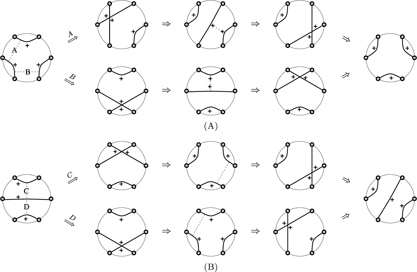
 , then switch the order of the hyperbolic singularities as in Figure 6. Since we have assumed that no other portions of the surface lie near the region of the contracted D, this isotopy is not obstructed by any other portion of the surface. This is an ambient isotopy near these singularities that fixes the boundary, and the resulting surface also admits an open book foliation. Figure 9a shows the open book foliations on each of the two surfaces; from these pictures, we can recover the surface, and we can also see that there are no more possible ways in which three leaves can merge through two hyperbolic singularities of the same sign. Figure 7 shows how the graphs change under the isotopy.
A motion picture view of the isotopy shown in Figure 6: (a) and (b) for singularities of the same orientation and (c) and (d) for singularities of opposite orientations. Dark dots are portions of the booklink, arcs are leaves labeled with orientation, and dotted lines show which leaves merge into singularities.

Figure 9 Long description
The diagram consists of two primary horizontal sequences, A and B, each showing topological transformations within circular frames.
In sequence A, the leftmost circle contains four dark dots on the perimeter connected by curved arcs labeled with plus signs. Dotted lines labeled A and B indicate merge paths. Following arrow A to the top row, three circles show a sequence where arcs shift and cross, with a dotted line indicating a leaf merging into a singularity. Following arrow B to the bottom row, a similar three-circle sequence shows arcs crossing at the bottom. Both paths converge to a final circle on the far right showing three arcs arranged symmetrically around the perimeter.
In sequence B, the leftmost circle shows a different initial configuration with a horizontal arc and dotted lines labeled C and D. Following arrow C to the top row, three circles depict the evolution of singularities with opposite orientations. Following arrow D to the bottom row, the sequence shows the merging of different leaves. Both paths in sequence B converge to a final circle on the far right featuring a central diagonal line crossing the circle, flanked by two curved arcs on the sides.
Throughout all panels, dark dots represent booklink portions, solid lines represent leaves with plus sign orientation labels, and dashed lines indicate the merging process into singularities.
Observe that this process was independent of the relative signs of the hyperbolic singularities precisely because the contractibility of D ensures that other portions of
$\Sigma $
 do not obstruct the move, even when the two singularities have opposite orientations.
4 A Markov theorem for book links
Finally, we may apply the techniques of Section 3 to understand how to use appropriate collections of annuli to generate book link isotopies (after suitable stabilization).
Proof of Theorem 1.2
Suppose
$\lambda _-$
 and
$\lambda _+$
 are book links of the same critical point type. By Lemma 2.1 there is a collection of book links
$\lambda _-=\lambda _0, \cdots , \lambda _n=\lambda _+$
 each of the same book link type interpolating between
$\lambda _-$
 and
$\lambda _+$
 together with collections of disjoint embedded annuli
$A_i$
 connecting
$\lambda _{i-1}$
 and
$\lambda _i$
 . It suffices to treat the case of a single annulus A bounded by book knots
$\lambda _-$
 and
$\lambda _+$
 and show how it generates a book link isotopy between suitably stabilized versions of the two book links.
We may assume by Lemma 3.1 that A has an open book foliation. We may also assume it only has
$\partial $
 - and h-tiles, possibly after applying a sequence of stabilizations to
$\lambda _-$
 and
$\lambda _+$
 , as in Lemma 3.2. Since A is an annulus, there is a separating cycle that passes some hyperbolic singularities of A and cuts it into two annular regions; equivalently, the graph
$\Gamma (A)$
 contains a single cycle. In what follows, we will alter the surface so that all h-tiles lie on this cycle and have one
$\partial $
 -tile on each side of it, that is, have one adjacent extremal singularity on each boundary component.
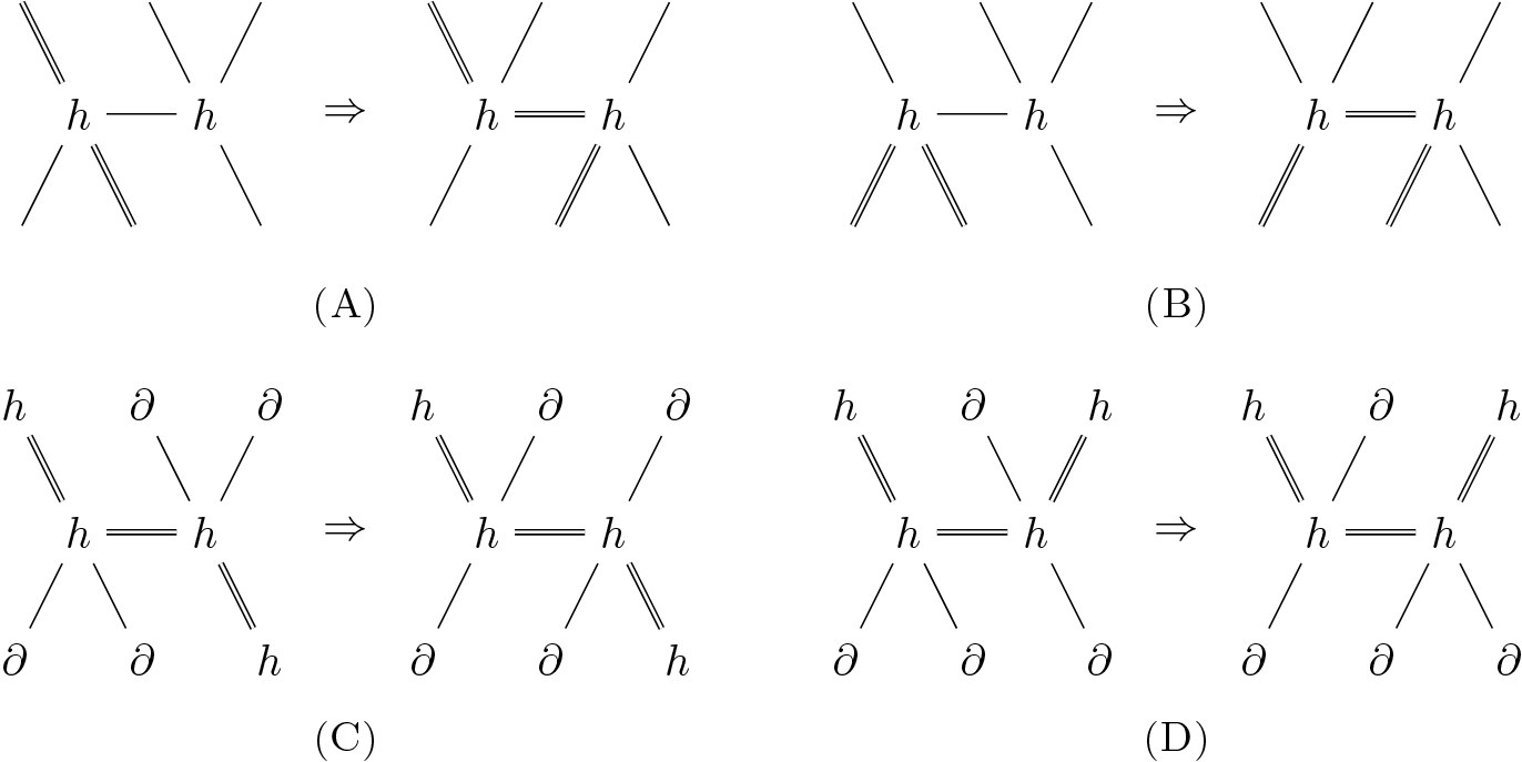
First, we will alter the surface inductively so that all h-tiles are adjacent to both boundary components, equivalently, so that all hyperbolic singularities are on the separating cycle in the annulus and their corresponding vertices lie in the single cycle in the graph. Let us first consider an h-tile that is adjacent to but not on the cycle, that is, which touches only one boundary component but is adjacent to an h-tile which touches both. Since one h-tile touches only one boundary component, it (and so each of its edges) cuts off a disk from the annulus, we may apply Lemma 3.3. See Figure 10a and 10b: the cycle (denoted by double edges in the figure) runs through one of the h-tiles but misses the other, so the isotopy will add the second h-tile to the cycle. From the point of view of the foliated surface, if one h-tile touches only one boundary component but is adjacent to a tile which touches both, then the transformation shifts one of the components to be shared by both h-tiles, and both tiles touch both components.
(a) and (b) Moving an h-tile onto the splitting cycle (marked by the double lines). (c) Changing two not-good h-tiles (with
$\partial $
 -tiles on the same side of the splitting cycle) into two good h-tiles (with
$\partial $
 -tiles across). (d) Moving a not-good h-tile along the splitting cycle.

Figure 10 Long description
The diagram consists of four panels labeled A through D. Each panel shows a before-and-after state separated by a double-lined arrow pointing right.
* Panel A: On the left, two h-nodes are connected by a single horizontal line. One h-node has a double-lined diagonal edge. On the right, the two h-nodes are now connected by a double horizontal line.
* Panel B: Similar to A, but the initial state shows two double-lined diagonal edges extending from the left h-node. The final state shows the h-nodes connected by a double horizontal line.
* Panel C: On the left, two h-nodes are connected by a double horizontal line. Various diagonal edges are labeled with the partial symbol. On the right, the configuration changes such that the partial symbols are positioned across the splitting cycle from each other.
* Panel D: Shows the movement of a not-good h-tile. On the left, two h-nodes are connected by a double horizontal line with partial symbols on diagonal edges. On the right, the h-tile has shifted along the double-lined splitting cycle, changing the distribution of the partial symbols on the surrounding edges.
Next, once all h-tiles fall in a single cycle, each must be adjacent to exactly two other h-tiles as well as two
$\partial $
 -tiles. We now ensure that each h-tile has its two
$\partial $
 -tiles across the singularity from one another and so on different boundary components. We will call such a hyperbolic tile a good tile. Recall that there are exactly
$\text{2}d$
 extremal singularities on each boundary component; so for each not-good tile with a pair of
$\partial $
 -tiles on
$\lambda _-$
 , there is another not-good tile with its pair of
$\partial $
 -tiles on
$\lambda _+$
 . If these two tiles are adjacent, then we apply Lemma 3.3 as in Figure 10c to move the
$\partial $
 -tiles and ensure they fall opposite one another across the h-tiles. On the other hand, if there are two such not-good tiles, but they are separated by good tiles, then we may still apply Lemma 3.3 to permute a not-good tile with a good tile until the pair of not-good tiles is adjacent, as in Figure 10d.
Finally, we may assume that there is a “necklace” of
$\text{2}d$
 of the h-tiles around the center of the annulus A, and each has two
$\partial $
 -vertices attached on opposite sides. In the braid case, the annulus was foliated entirely by non-singular arcs connecting the two boundary components, provided a recipe for pushing
$\lambda _-$
 along the surface, each point following the appropriate non-singular arc to
$\lambda _+$
 ; this was an isotopy, and it did not introduce any critical points. Similarly, an h-tile with its pair of
$\partial $
 -tiles on opposite boundary component foliation suggests a method for pushing
$\lambda _-$
 smoothly across the tile to
$\lambda _+$
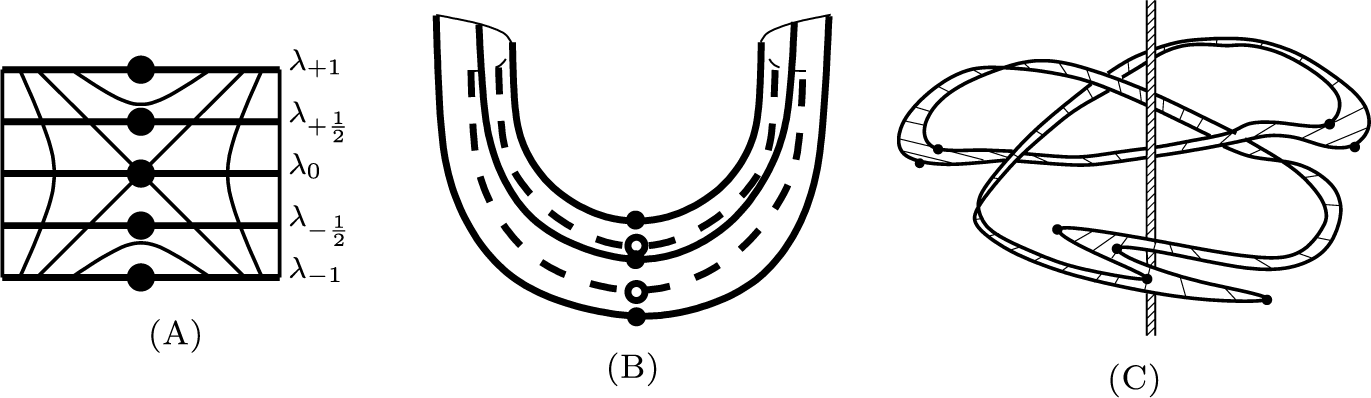
 , maintaining the critical point all along (see Figure 11a and b).
Remark 4.1 The methods of the proof above may be applied to any surface bounded by a book link: it may be perturbed or stabilized to remove all tiles except
$\partial $
 - and h-tiles, and these may then be rearranged, with some restrictions. Additionally, each of the h-tiles with an adjacent
$\partial $
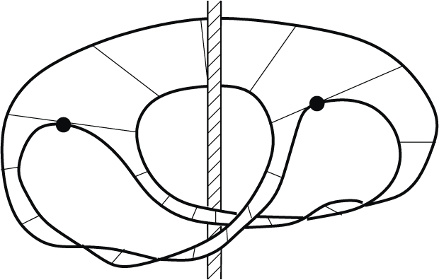
 -tile may be resolved in the reverse of Figure 5a; in the case of the annulus arising in the proof of the theorem, this will remove all the h-tiles and result in a surface such as Figure 11c. For another example, see Figure 12 for a Seifert surface for the trefoil with an open book foliation and resolved to contain only extremal singularities and their tiles.
(a and b) An isotopy
$\lambda _t$
 generated by an h-tile with a pair of
$\partial $
 -tiles. (c) A foliated annulus between book knots consisting only of tiles with extremal critical points.

Figure 11 Long description
Panel A shows a rectangular grid with five horizontal lines. Each line has a central black dot. From top to bottom, the lines are labeled lambda sub plus 1, lambda sub plus 1 over 2, lambda sub 0, lambda sub minus 1 over 2, and lambda sub minus 1. Curved lines intersect these horizontal lines, forming a saddle-like pattern around the central lambda sub 0 point. Panel B depicts a U-shaped curved band containing three concentric solid black curves and two dashed curves. Four points are marked at the base of the U-shaped curved band: two solid black dots on the outermost and innermost solid lines, and two open circles on the intermediate dashed and solid lines. Panel C illustrates a complex, knotted foliated annulus. It consists of a ribbon-like structure with diagonal hatching that twists around a vertical hatched axis. Several small black dots are placed at extremal points along the ribbon's curves to indicate critical points.
An open book foliation containing only extremal critical points.

Acknowledgements
This project began at the AMS North Central Sectional Meeting at Creighton University in Fall 2023. We would like to thank the organizers of this meeting and its special sessions. We also thank the referee, who pointed out an error in a lemma in a previous version of this article.












 Open access

