1 Introduction
The eigenvalues of the Laplacian have been the object of intensive study over the last century. Of particular interest are related shape optimization problems. For
 $k\in \mathbb{N}$
, the goal is to optimize the
 $k$
th eigenvalue of the Laplacian with boundary conditions over a collection of open sets in
 $\mathbb{R}^{m}$
. This collection satisfies geometric constraints, such as fixed Lebesgue measure or fixed perimeter.
For an open set
 $\unicode[STIX]{x1D6FA}\subset \mathbb{R}^{m}$
,
 $m\geqslant 2$
, of finite Lebesgue measure
 $|\unicode[STIX]{x1D6FA}|$
, we let
 $\unicode[STIX]{x1D706}_{k}(\unicode[STIX]{x1D6FA})$
,
 $k\in \mathbb{N}$
, denote the Dirichlet eigenvalues of the Laplacian on
 $\unicode[STIX]{x1D6FA}$
which are strictly positive, arranged in non-decreasing order and counted with multiplicity: that is,
 $$\begin{eqnarray}\displaystyle \unicode[STIX]{x1D706}_{1}(\unicode[STIX]{x1D6FA})\leqslant \unicode[STIX]{x1D706}_{2}(\unicode[STIX]{x1D6FA})\leqslant \unicode[STIX]{x1D706}_{3}(\unicode[STIX]{x1D6FA})\leqslant \cdots \leqslant \unicode[STIX]{x1D706}_{k}(\unicode[STIX]{x1D6FA})\leqslant \cdots \,. & & \displaystyle \nonumber\end{eqnarray}$$
This sequence accumulates at
 $+\infty$
.
We consider the minimization problem given by
 $$\begin{eqnarray}\unicode[STIX]{x1D706}_{k}^{\ast }(m):=\inf \{\unicode[STIX]{x1D706}_{k}(\unicode[STIX]{x1D6FA}):\unicode[STIX]{x1D6FA}\text{ open in }\mathbb{R}^{m},|\unicode[STIX]{x1D6FA}|=c\}.\end{eqnarray}$$
It was shown by Faber and Krahn that among all open sets in
 $\mathbb{R}^{m}$
of measure
 $c$
, the ball of measure
 $c$
minimizes the first Dirichlet eigenvalue (see [Reference Henrot15]). Krahn and Szego proved that, among all open sets in
 $\mathbb{R}^{m}$
of measure
 $c$
, the second Dirichlet eigenvalue is minimized by the union of two disjoint balls of measure
 $c/2$
each (see [Reference Henrot15]). For
 $k\geqslant 3$
, the existence of an open set of prescribed measure which minimizes the
 $k$
th Dirichlet eigenvalue remains unresolved to date. However, in the class of quasi-open sets of prescribed measure, it was shown by Bucur in [Reference Bucur7] that a minimizer does exist and that such a minimizer is bounded and has finite perimeter. Independently, Mazzoleni and Pratelli, in [Reference Mazzoleni and Pratelli17], proved the existence of a minimizer in the collection of quasi-open sets. For any lower semi-continuous, increasing function of the first
 $k$
Dirichlet eigenvalues, they proved the existence of a minimizer which is bounded in terms of
 $k$
and
 $m$
independently of the function. It was shown in [Reference van den Berg and Iversen5] that, for
 $k\leqslant m+1$
, any bounded minimizer of
 $\unicode[STIX]{x1D706}_{k}(\unicode[STIX]{x1D6FA})$
has at most
 $\min \{7,k\}$
components.
No optimal domains are known for
 $\unicode[STIX]{x1D706}_{k}$
with
 $k\geqslant 3$
. In particular, the conjecture that if
 $m=2$
, then
 $\unicode[STIX]{x1D706}_{3}(\unicode[STIX]{x1D6FA})$
is bounded from below by the third eigenvalue of the disc with the same measure as
 $\unicode[STIX]{x1D6FA}$
is open. There are no obvious candidates for minimizers of
 $\unicode[STIX]{x1D706}_{k}$
with
 $k\geqslant 5$
in any dimension
 $m\geqslant 2$
. Even for
 $m=2$
, minimizers need not be discs or disjoint unions of discs (see [Reference Wolf and Keller21]). Furthermore, it was shown in [Reference Berger6] that, for
 $k\geqslant 5$
,
 $\unicode[STIX]{x1D706}_{k}(\unicode[STIX]{x1D6FA})$
cannot be minimized by a disc or a disjoint union of discs. The numerical investigation [Reference Antunes and Freitas1] suggests that for some values of
 $k$
the minimizers may not have any symmetries.
Pólya’s conjecture for Dirichlet eigenvalues asserts that for all bounded, open sets
 $\unicode[STIX]{x1D6FA}\subset \mathbb{R}^{m}$
,
 $\unicode[STIX]{x1D706}_{k}(\unicode[STIX]{x1D6FA})\geqslant 4\unicode[STIX]{x1D70B}^{2}(\unicode[STIX]{x1D714}_{m}|\unicode[STIX]{x1D6FA}|)^{-2/m}k^{2/m}$
, where
 $\unicode[STIX]{x1D714}_{m}$
denotes the measure of a ball in
 $\mathbb{R}^{m}$
of radius 1. It was shown in [Reference Colbois and El Soufi11] that Pólya’s conjecture is equivalent to
 $\unicode[STIX]{x1D706}_{k}^{\ast }(m)$
being asymptotically equal to
 $4\unicode[STIX]{x1D70B}^{2}(\unicode[STIX]{x1D714}_{m}c)^{-2/m}k^{2/m}$
as
 $k\rightarrow \infty$
.
It is also interesting to consider the optimization of the eigenvalues of the Laplacian subject to other geometric constraints, such as fixed perimeter. For the Dirichlet eigenvalues, existence of a minimizer in the class of open sets in
 $\mathbb{R}^{m}$
of finite Lebesgue measure and prescribed perimeter was shown in [Reference De Philippis and Velichkov12]. Moreover, it was shown there that any minimizer is bounded and connected, and regularity results for the boundary were also obtained. Bucur and Freitas, in [Reference Bucur and Freitas9], showed that any sequence of minimizers of
 $\unicode[STIX]{x1D706}_{k}$
in
 $\mathbb{R}^{2}$
with perimeter
 $\ell$
converges in the sense of Hausdorff to the disc of perimeter
 $\ell$
as
 $k\rightarrow \infty$
. They also showed that if the collection of admissible sets is restricted to the collection of
 $n$
-sided, convex, planar polygons of perimeter
 $\ell$
, then any sequence of minimizers converges to the regular
 $n$
-sided polygon of perimeter
 $\ell$
as
 $k\rightarrow \infty$
. For
 $m\geqslant 2$
, other constraints were considered in [Reference van den Berg4], including perimeter and moment of inertia, subject to an additional convexity constraint. Further results for the Dirichlet eigenvalues were obtained in [Reference Antunes and Freitas3], [Reference Bucur, Buttazzo and Henrot8], [Reference van den Berg and Iversen5], [Reference Bucur and Freitas9] and [Reference van den Berg4]. Some of the results of [Reference Antunes and Freitas3] follow directly from those in [Reference van den Berg4], while the results of [Reference De Philippis and Velichkov12] supersede those of [Reference Bucur, Buttazzo and Henrot8].
Recently, Antunes and Freitas considered the problem of minimizing
 $\unicode[STIX]{x1D706}_{k}$
over all planar rectangles of unit measure (see [Reference Antunes and Freitas2]). In [Reference Antunes and Freitas2, Theorem 2.1], they showed that any sequence of minimizing rectangles for the Dirichlet eigenvalues converges to the unit square in the sense of Hausdorff as
 $k\rightarrow \infty$
.
In Theorem 1.1 below, we obtain the corresponding three-dimensional result for the Dirichlet eigenvalues of the Laplacian on cuboids in
 $\mathbb{R}^{3}$
of unit measure. In addition, we obtain an estimate for the rate of convergence. Let
 $R_{a_{1},a_{2},a_{3}}$
denote a cuboid in
 $\mathbb{R}^{3}$
of side lengths
 $a_{1},a_{2},a_{3}$
such that
 $a_{1}a_{2}a_{3}=1$
and
 $a_{1}\leqslant a_{2}\leqslant a_{3}$
: that is,
 $$\begin{eqnarray}\displaystyle R_{a_{1},a_{2},a_{3}} & = & \displaystyle \{(x_{1},x_{2},x_{3})\in \mathbb{R}^{3}:0<x_{1}<a_{1},\nonumber\\ \displaystyle & & \displaystyle \quad 0<x_{2}<a_{2},0<x_{3}<(a_{1}a_{2})^{-1},a_{1}\leqslant a_{2}\leqslant a_{3}\!\}.\end{eqnarray}$$
We prove the following theorem.
Theorem 1.1. (i) Let
 $k\in \mathbb{N}$
. The variational problem
 $$\begin{eqnarray}\displaystyle \unicode[STIX]{x1D706}_{k}^{\ast }:=\inf \{\unicode[STIX]{x1D706}_{k}(R_{a_{1},a_{2},a_{3}}):a_{1}\leqslant a_{2}\leqslant a_{3}\} & & \displaystyle \nonumber\end{eqnarray}$$
has an optimal cuboid
 $R_{a_{1,k}^{\ast },a_{2,k}^{\ast },a_{3,k}^{\ast }}$
with side lengths
 $a_{1,k}^{\ast }\leqslant a_{2,k}^{\ast }\leqslant a_{3,k}^{\ast }$
such that
 $a_{1,k}^{\ast }a_{2,k}^{\ast }a_{3,k}^{\ast }=1.$
-
(ii)
(1.2)where $$\begin{eqnarray}\displaystyle a_{3,k}^{\ast }\leqslant 1+O(k^{-(2-\unicode[STIX]{x1D6FD})/6}),\quad k\rightarrow \infty , & & \displaystyle\end{eqnarray}$$
$\unicode[STIX]{x1D6FD}$
is an exponent of the remainder in Furthermore, any sequence of optimal cuboids
$$\begin{eqnarray}\#\{(i_{1},i_{2},i_{3})\in \mathbb{Z}^{3}:i_{1}^{2}+i_{2}^{2}+i_{3}^{2}\leqslant R^{2}\}-\frac{4\unicode[STIX]{x1D70B}}{3}R^{3}=O(R^{\unicode[STIX]{x1D6FD}}),\quad R\rightarrow \infty .\end{eqnarray}$$
$R_{a_{1,k}^{\ast },a_{2,k}^{\ast },a_{3,k}^{\ast }}$
converges to the unit cube in
$\mathbb{R}^{3}$
in the sense of Hausdorff as
$k\rightarrow \infty$
.


The best estimate known to date is that, for any
 $\unicode[STIX]{x1D716}>0,\unicode[STIX]{x1D6FD}=\frac{21}{16}+\unicode[STIX]{x1D716}$
(see [Reference Heath-Brown14]). Hence (1.2) holds for
 $\unicode[STIX]{x1D6FD}=\frac{21}{16}+\unicode[STIX]{x1D716},\unicode[STIX]{x1D716}>0$
. The conjecture for the optimal remainder is
 $\unicode[STIX]{x1D6FD}=1+\unicode[STIX]{x1D716},\unicode[STIX]{x1D716}>0$
(see [Reference Chamizo and Pastor10]).
A heuristic explanation for this asymptotic shape result is the following (see also [Reference Antunes and Freitas2]). For any cuboid
 $R$
in
 $\mathbb{R}^{3}$
with measure
 $|R|$
and perimeter
 $\text{Per}(R)$
,
 $$\begin{eqnarray}\displaystyle \unicode[STIX]{x1D706}_{k}(R)=\biggl(\frac{6\unicode[STIX]{x1D70B}^{2}k}{|R|}\biggr)^{2/3}+\frac{(3\unicode[STIX]{x1D70B}^{5})^{1/3}\text{Per}(R)k^{1/3}}{2^{5/3}|R|^{4/3}}+o(k^{1/3}),\quad k\rightarrow \infty . & & \displaystyle\end{eqnarray}$$
So, if
 $|R|=1$
, then (1.3) suggests that the cuboid that minimizes
 $\unicode[STIX]{x1D706}_{k}(R)$
,
 $k\rightarrow \infty ,$
is the one with minimal perimeter, that is, the unit cube.
The Dirichlet eigenvalues of the Laplacian on a cuboid
 $R_{a_{1},a_{2},a_{3}}$
(as in (1.1)) are given by
 $$\begin{eqnarray}\displaystyle \frac{\unicode[STIX]{x1D70B}^{2}i_{1}^{2}}{a_{1}^{2}}+\frac{\unicode[STIX]{x1D70B}^{2}i_{2}^{2}}{a_{2}^{2}}+\frac{\unicode[STIX]{x1D70B}^{2}i_{3}^{2}}{a_{3}^{2}},\quad i_{1},i_{2},i_{3}\in \mathbb{N}. & & \displaystyle\end{eqnarray}$$
By listing these in non-decreasing order including multiplicities, the
 $k$
th Dirichlet eigenvalue on
 $R_{a_{1},a_{2},a_{3}}$
,
 $\unicode[STIX]{x1D706}_{k}(R_{a_{1},a_{2},a_{3}})$
, is the
 $k$
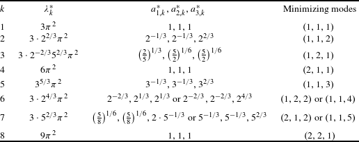
th item of this list. In Table 1, we list the optimal cuboids for the first few Dirichlet eigenvalues.
The first eight minimized Dirichlet eigenvalues, the side lengths of the cuboids that realize them, and the corresponding minimizing modes.

Let
 $\unicode[STIX]{x1D706}\in \mathbb{R}$
, let
 $\unicode[STIX]{x1D706}\geqslant 0$
and let
 $a_{1},a_{2},a_{3}\in \mathbb{R}$
be such that
 $a_{1}a_{2}a_{3}=1$
and
 $a_{1}\leqslant a_{2}\leqslant a_{3}$
. With (1.4) in mind, we define
 $$\begin{eqnarray}\displaystyle E(\unicode[STIX]{x1D706}):=\biggl\{(x_{1},x_{2},x_{3})\in \mathbb{R}^{3}:\frac{x_{1}^{2}}{a_{1}^{2}}+\frac{x_{2}^{2}}{a_{2}^{2}}+\frac{x_{3}^{2}}{a_{3}^{2}}\leqslant \frac{\unicode[STIX]{x1D706}}{\unicode[STIX]{x1D70B}^{2}}\biggr\}. & & \displaystyle\end{eqnarray}$$
The ellipsoid
 $E(\unicode[STIX]{x1D706})$
has semi-axes
 $$\begin{eqnarray}\displaystyle r_{1}=\frac{a_{1}\unicode[STIX]{x1D706}^{1/2}}{\unicode[STIX]{x1D70B}},\qquad r_{2}=\frac{a_{2}\unicode[STIX]{x1D706}^{1/2}}{\unicode[STIX]{x1D70B}},\qquad r_{3}=\frac{a_{3}\unicode[STIX]{x1D706}^{1/2}}{\unicode[STIX]{x1D70B}}, & & \displaystyle \nonumber\end{eqnarray}$$
and
 $|E(\unicode[STIX]{x1D706})|=(4/3\unicode[STIX]{x1D70B}^{2})\unicode[STIX]{x1D706}^{3/2}$
.
By (1.4) and (1.5), we see that the Dirichlet eigenvalues
 $\unicode[STIX]{x1D706}_{1}(R_{a_{1},a_{2},a_{3}}),\ldots ,\unicode[STIX]{x1D706}_{k}(R_{a_{1},a_{2},a_{3}})$
(counted with multiplicities) correspond to the integer lattice points that are inside or on the ellipsoid
 $E(\unicode[STIX]{x1D706}_{k})$
in the first octant (excluding the coordinate planes). Thus, in order to minimize
 $\unicode[STIX]{x1D706}_{k}$
among all cuboids given by (1.1), we wish to determine the three-dimensional ellipsoid
 $E(\unicode[STIX]{x1D706})$
of minimal measure which encloses
 $k$
integer lattice points in the first octant (excluding the coordinate planes).
For
 $n\in \mathbb{N}$
,
 $n\geqslant 2$
, estimates for the number of integer lattice points which are inside or on an
 $n$
-dimensional ellipsoid have been widely studied from a number-theoretical viewpoint. However, in order to use these estimates, it is crucial that the corresponding cuboids are bounded as
 $k\rightarrow \infty$
. As in the two-dimensional case, this is the most difficult part of the proof.
This paper is organized as follows. In §2, we prove Theorem 1.1(i). In §3, we obtain bounds for lattice point sums which are key ingredients in the proofs of the lemmas in §4. In that section, we follow the strategy of [Reference Antunes and Freitas2] and prove that the side lengths of a sequence of minimal cuboids
 $(R_{a_{1,k}^{\ast },a_{2,k}^{\ast },a_{3,k}^{\ast }})_{k}$
are bounded uniformly in
 $k$
. This is achieved by first obtaining an upper bound for the counting function
 $N(\unicode[STIX]{x1D706})=\#\{j\in \mathbb{N}:\unicode[STIX]{x1D706}_{j}(R_{a_{1},a_{2},a_{3}})\leqslant \unicode[STIX]{x1D706}\}$
for arbitrary cuboids. Using the maximality of
 $R_{a_{1,k}^{\ast },a_{2,k}^{\ast },a_{3,k}^{\ast }}$
and comparing with the unit cube gives the required uniform bound. Finally, in §5, we use known estimates for the number of integer lattice points that are inside and on an ellipsoid to conclude the proof of Theorem 1.1(ii).
2 Proof of Theorem 1.1(i)
Proof. Fix
 $k\in \mathbb{N}$
. Suppose that
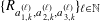 $\{R_{a_{1,k}^{(\ell )},a_{2,k}^{(\ell )},a_{3,k}^{(\ell )}}\}_{\ell \in \mathbb{N}}$
is a minimizing sequence for
 $\unicode[STIX]{x1D706}_{k}$
such that
 $a_{3,k}^{(\ell )}\rightarrow \infty$
as
 $\ell \rightarrow \infty$
. In order to preserve the measure constraint,
 $a_{1,k}^{(\ell )}\rightarrow 0$
as
 $\ell \rightarrow \infty$
. So
 $$\begin{eqnarray}\displaystyle \unicode[STIX]{x1D706}_{k}(R_{a_{1,k}^{(\ell )},a_{2,k}^{(\ell )},a_{3,k}^{(\ell )}})>\frac{\unicode[STIX]{x1D70B}^{2}}{(a_{1,k}^{(\ell )})^{2}}\rightarrow \infty \quad \text{as }\ell \rightarrow \infty . & & \displaystyle \nonumber\end{eqnarray}$$
However, for the unit cube in
 $\mathbb{R}^{3}$
,
 $\unicode[STIX]{x1D706}_{k}\leqslant 3\unicode[STIX]{x1D70B}^{2}k^{2}<+\infty$
. This contradicts the assumption that
 $\{R_{a_{1,k}^{(\ell )},a_{2,k}^{(\ell )},a_{3,k}^{(\ell )}}\}_{\ell \in \mathbb{N}}$
is a minimizing sequence for
 $\unicode[STIX]{x1D706}_{k}$
. So any minimizing sequence
 $\{R_{a_{1,k}^{(\ell )},a_{2,k}^{(\ell )},a_{3,k}^{(\ell )}}\}_{\ell \in \mathbb{N}}$
for
 $\unicode[STIX]{x1D706}_{k}$
is such that
 $a_{1,k}^{(\ell )},a_{2,k}^{(\ell )},a_{3,k}^{(\ell )}$
are bounded as
 $\ell \rightarrow \infty$
. Hence, for each
 $i\in \{1,2,3\}$
, there exists a convergent subsequence, again denoted by
 $a_{i,k}^{(\ell )}$
, such that
 $a_{i,k}^{(\ell )}\rightarrow a_{i,k}^{\ast }$
for some
 $a_{i,k}^{\ast }\in (0,\infty )$
. Since
 $(a_{1},a_{2},a_{3})\mapsto \unicode[STIX]{x1D706}_{k}(R_{a_{1},a_{2},a_{3}})$
is continuous,
 $\unicode[STIX]{x1D706}_{k}(R_{a_{1,k}^{(\ell )},a_{2,k}^{(\ell )},a_{3,k}^{(\ell )}})\rightarrow \unicode[STIX]{x1D706}_{k}(R_{a_{1,k}^{\ast },a_{2,k}^{\ast },a_{3,k}^{\ast }})$
as
 $\ell \rightarrow \infty$
. Hence
 $R_{a_{1,k}^{\ast },a_{2,k}^{\ast },a_{3,k}^{\ast }}$
is an optimal cuboid for
 $\unicode[STIX]{x1D706}_{k}$
.◻
It is not difficult to see that the above argument can also be used to prove the existence of an optimal cuboid for
 $\unicode[STIX]{x1D706}_{k}$
in
 $\mathbb{R}^{m}$
with
 $m\geqslant 4$
.
3 Key lemmas to prove boundedness of an optimal cuboid
The following lemmas are crucial in the proofs that follow in §4.
Lemma 3.1. Let
 $y\geqslant 0$
,
 $a\geqslant 0$
. For
 $n\in \{1,2\}$
,
 $$\begin{eqnarray}\displaystyle \mathop{\sum }_{i=1}^{\lfloor y^{1/2}/a\rfloor }(y-a^{2}i^{2})^{n/2} & {\leqslant} & \displaystyle \frac{\sqrt{\unicode[STIX]{x1D70B}}}{2a}\frac{\unicode[STIX]{x1D6E4}((n+2)/2)}{\unicode[STIX]{x1D6E4}((n+3)/2)}y^{(n+1)/2}\nonumber\\ \displaystyle & & \displaystyle -\,\frac{1}{2}y^{n/2}+\frac{(2an)^{n/2}}{(n+2)^{(n+2)/2}}y^{n/4}.\end{eqnarray}$$
Proof. We know that
 $$\begin{eqnarray}\displaystyle \mathop{\sum }_{i=1}^{\lfloor y^{1/2}/a\rfloor }(y-a^{2}i^{2})^{n/2}=a^{n}\mathop{\sum }_{i=1}^{\lfloor y^{1/2}/a\rfloor }\biggl(\biggl(\frac{y^{1/2}}{a}\biggr)^{2}-i^{2}\biggr)^{n/2}. & & \displaystyle\end{eqnarray}$$
Let
 $R=y^{1/2}/a$
and consider
 $\sum _{i=1}^{\lfloor R\rfloor }g(i)$
, where
 $$\begin{eqnarray}\displaystyle g(i)=(R^{2}-i^{2})^{n/2}. & & \displaystyle\end{eqnarray}$$
Then, for
 $0\leqslant i\leqslant R$
,
 $$\begin{eqnarray}\displaystyle & g^{\prime }(i)=-ni(R^{2}-i^{2})^{(n-2)/2}\leqslant 0, & \displaystyle \nonumber\\ \displaystyle & g^{\prime \prime }(i)=n(R^{2}-i^{2})^{(n-4)/2}((n-1)i^{2}-R^{2})\leqslant 0. & \displaystyle \nonumber\end{eqnarray}$$
So
 $i\mapsto g(i)$
is decreasing on
 $[0,R]$
and, since
 $n=1$
or
 $n=2$
,
 $g$
is also concave on
 $[0,R]$
. We note that since
 $g$
is decreasing,
 $\sum _{i=1}^{\lfloor R\rfloor }g(i)$
is the total area of the rectangles of width 1 and height
 $g(i)$
,
 $i\in \{1,\ldots ,\lfloor R\rfloor \}$
which are inscribed in the curve
 $g(x)$
for
 $0\leqslant x\leqslant R$
. Due to the concavity of
 $g$
on
 $(0,R)$
, we can bound
 $\sum _{i=1}^{\lfloor R\rfloor }g(i)$
from above by the area under
 $g$
minus the area of the inscribed triangles that sit on top of the aforementioned rectangles: that is,
 $$\begin{eqnarray}\displaystyle \mathop{\sum }_{i=1}^{\lfloor R\rfloor }g(i)\leqslant \int _{0}^{R}g(i)\,di-\frac{1}{2}\mathop{\sum }_{i=1}^{\lfloor R\rfloor }(g(i-1)-g(i))-\frac{1}{2}(R-\lfloor R\rfloor )g(\lfloor R\rfloor ). & & \displaystyle\end{eqnarray}$$
We know that
 $$\begin{eqnarray}\displaystyle \int _{0}^{R}g(i)\,di & = & \displaystyle R^{n+1}\int _{0}^{1}(1-t^{2})^{n/2}\,dt\nonumber\\ \displaystyle & = & \displaystyle \frac{R^{n+1}}{2}\int _{0}^{1}(1-s)^{n/2}\frac{1}{\sqrt{s}}\,ds=\frac{\sqrt{\unicode[STIX]{x1D70B}}}{2}\frac{\unicode[STIX]{x1D6E4}((n+2)/2)}{\unicode[STIX]{x1D6E4}((n+3)/2)}R^{n+1},\quad\end{eqnarray}$$
where we have used [Reference Gradshteyn and Ryzhik13, 3.191.3, 8.384.1].
We also know that
 $$\begin{eqnarray}\displaystyle & & \displaystyle -\frac{1}{2}\mathop{\sum }_{i=1}^{\lfloor R\rfloor }(g(i-1)-g(i))-\frac{1}{2}(R-\lfloor R\rfloor )g(\lfloor R\rfloor )\nonumber\\ \displaystyle & & \displaystyle \quad =-\frac{1}{2}R^{n}+\frac{1}{2}(1+\lfloor R\rfloor -R)(R^{2}-\lfloor R\rfloor ^{2})^{n/2}\nonumber\\ \displaystyle & & \displaystyle \quad =-\frac{1}{2}R^{n}+\frac{1}{2}(1+\lfloor R\rfloor -R)(R+\lfloor R\rfloor )^{n/2}(R-\lfloor R\rfloor )^{n/2}\nonumber\\ \displaystyle & & \displaystyle \quad \leqslant -\frac{1}{2}R^{n}+\frac{1}{2}(2R)^{n/2}\max _{0\leqslant \unicode[STIX]{x1D6FD}<1}(1-\unicode[STIX]{x1D6FD})\unicode[STIX]{x1D6FD}^{n/2}\nonumber\\ \displaystyle & & \displaystyle \quad =-\frac{1}{2}R^{n}+\frac{(2n)^{n/2}}{(n+2)^{(n+2)/2}}R^{n/2}.\end{eqnarray}$$
Applying the previous lemma with
 $n=1$
,
 $y=(a_{2}^{2}/\unicode[STIX]{x1D70B}^{2})\unicode[STIX]{x1D706}$
and
 $a=a_{2}/a_{1}$
, we recover the result of [Reference Antunes and Freitas2, Theorem 3.1]. Since
 $g$
(as in (3.3)) is decreasing on
 $[0,y^{1/2}/a]$
, the following lemma holds for all
 $n\in \mathbb{N}$
.
Lemma 3.2. Let
 $y\geqslant 0$
,
 $a\geqslant 0$
. For
 $n\in \mathbb{N}$
,
 $$\begin{eqnarray}\displaystyle \mathop{\sum }_{i=1}^{\lfloor y^{1/2}/a\rfloor }(y-a^{2}i^{2})^{n/2}\leqslant \int _{0}^{y^{1/2}/a}(y-a^{2}i^{2})^{n/2}\,di=\frac{\sqrt{\unicode[STIX]{x1D70B}}}{2a}\frac{\unicode[STIX]{x1D6E4}((n+2)/2)}{\unicode[STIX]{x1D6E4}((n+3)/2)}y^{(n+1)/2}. & & \displaystyle \nonumber\end{eqnarray}$$
4 Uniform boundedness of an optimal cuboid
With
 $E(\unicode[STIX]{x1D706})$
as defined in (1.5), we define the counting function
 $$\begin{eqnarray}\displaystyle N(\unicode[STIX]{x1D706}):=\#\{j\in \mathbb{N}:\unicode[STIX]{x1D706}_{j}(R_{a_{1},a_{2},a_{3}})\leqslant \unicode[STIX]{x1D706}\}=\#\{(i_{1},i_{2},i_{3})\in \mathbb{N}^{3}\cap E(\unicode[STIX]{x1D706})\}. & & \displaystyle \nonumber\end{eqnarray}$$
We now use the results of §3 to obtain an upper bound for
 $N(\unicode[STIX]{x1D706})$
.
Lemma 4.1. For
 $\unicode[STIX]{x1D706}\geqslant 0$
and
 $a_{1}\leqslant a_{2}\leqslant a_{3}$
,
 $E(\unicode[STIX]{x1D706})$
and
 $N(\unicode[STIX]{x1D706})$
as above,
 $$\begin{eqnarray}\displaystyle N(\unicode[STIX]{x1D706})\leqslant \frac{\unicode[STIX]{x1D706}^{3/2}}{6\unicode[STIX]{x1D70B}^{2}}-\frac{\unicode[STIX]{x1D706}}{8\unicode[STIX]{x1D70B}a_{1}}+\frac{\unicode[STIX]{x1D706}^{1/2}}{16a_{1}^{2}}. & & \displaystyle\end{eqnarray}$$
Proof. For
 $(i_{1},i_{2},i_{3})\in \mathbb{N}^{3}\cap E(\unicode[STIX]{x1D706})$
,
 $$\begin{eqnarray}\displaystyle i_{3}\leqslant \biggl\lfloor\biggl(\frac{a_{3}^{2}}{\unicode[STIX]{x1D70B}^{2}}\unicode[STIX]{x1D706}-\frac{a_{3}^{2}}{a_{1}^{2}}i_{1}^{2}-\frac{a_{3}^{2}}{a_{2}^{2}}i_{2}^{2}\biggr)_{+}^{1/2}\biggr\rfloor, & & \displaystyle \nonumber\end{eqnarray}$$
where “
 $+$
” denotes the positive part. Hence
 $$\begin{eqnarray}\displaystyle N(\unicode[STIX]{x1D706}) & {\leqslant} & \displaystyle \mathop{\sum }_{i_{1}\in \mathbb{N}}\mathop{\sum }_{i_{2}\in \mathbb{N}}\biggl\lfloor\biggl(\frac{a_{3}^{2}}{\unicode[STIX]{x1D70B}^{2}}\unicode[STIX]{x1D706}-\frac{a_{3}^{2}}{a_{1}^{2}}i_{1}^{2}-\frac{a_{3}^{2}}{a_{2}^{2}}i_{2}^{2}\biggr)_{+}^{1/2}\biggr\rfloor\end{eqnarray}$$
 $$\begin{eqnarray}\displaystyle & {\leqslant} & \displaystyle \mathop{\sum }_{i_{1}=1}^{\lfloor a_{1}(\unicode[STIX]{x1D706}^{1/2}/\unicode[STIX]{x1D70B})\rfloor }\mathop{\sum }_{i_{2}=1}^{\lfloor a_{2}(\unicode[STIX]{x1D706}/\unicode[STIX]{x1D70B}^{2}-i_{1}^{2}/a_{1}^{2})^{1/2}\rfloor }\biggl(\frac{a_{3}^{2}}{\unicode[STIX]{x1D70B}^{2}}\unicode[STIX]{x1D706}-\frac{a_{3}^{2}}{a_{1}^{2}}i_{1}^{2}-\frac{a_{3}^{2}}{a_{2}^{2}}i_{2}^{2}\biggr)^{1/2}.\end{eqnarray}$$
Applying Lemma 3.2 with
 $y=(a_{3}^{2}/\unicode[STIX]{x1D70B}^{2})\unicode[STIX]{x1D706}-(a_{3}^{2}/a_{1}^{2})i_{1}^{2}$
,
 $a=a_{3}/a_{2}$
,
 $n=1$
to (4.3), gives
 $$\begin{eqnarray}\displaystyle N(\unicode[STIX]{x1D706}) & {\leqslant} & \displaystyle \mathop{\sum }_{i_{1}=1}^{\lfloor a_{1}(\unicode[STIX]{x1D706}^{1/2}/\unicode[STIX]{x1D70B})\rfloor }\frac{\unicode[STIX]{x1D70B}a_{2}}{4a_{3}}\biggl(\frac{a_{3}^{2}}{\unicode[STIX]{x1D70B}^{2}}\unicode[STIX]{x1D706}-\frac{a_{3}^{2}}{a_{1}^{2}}i_{1}^{2}\biggr)\nonumber\\ \displaystyle & = & \displaystyle \mathop{\sum }_{i_{1}=1}^{\lfloor a_{1}(\unicode[STIX]{x1D706}^{1/2}/\unicode[STIX]{x1D70B})\rfloor }\frac{\unicode[STIX]{x1D70B}a_{2}a_{3}}{4}\biggl(\frac{\unicode[STIX]{x1D706}}{\unicode[STIX]{x1D70B}^{2}}-\frac{i_{1}^{2}}{a_{1}^{2}}\biggr).\end{eqnarray}$$
Applying Lemma 3.1 with
 $y=\unicode[STIX]{x1D706}/\unicode[STIX]{x1D70B}^{2}$
,
 $a=1/a_{1}$
,
 $n=2$
, we obtain that
 $$\begin{eqnarray}\displaystyle \frac{\unicode[STIX]{x1D70B}a_{2}a_{3}}{4}\mathop{\sum }_{i_{1}=1}^{\lfloor a_{1}(\unicode[STIX]{x1D706}^{1/2}/\unicode[STIX]{x1D70B})\rfloor }\biggl(\frac{\unicode[STIX]{x1D706}}{\unicode[STIX]{x1D70B}^{2}}-\frac{i_{1}^{2}}{a_{1}^{2}}\biggr) & {\leqslant} & \displaystyle \frac{\unicode[STIX]{x1D70B}a_{2}a_{3}}{4}\biggl(\frac{2a_{1}}{3\unicode[STIX]{x1D70B}^{3}}\unicode[STIX]{x1D706}^{3/2}-\frac{1}{2\unicode[STIX]{x1D70B}^{2}}\unicode[STIX]{x1D706}+\frac{1}{4\unicode[STIX]{x1D70B}a_{1}}\unicode[STIX]{x1D706}^{1/2}\biggr)\nonumber\\ \displaystyle & = & \displaystyle \frac{\unicode[STIX]{x1D706}^{3/2}}{6\unicode[STIX]{x1D70B}^{2}}-\frac{\unicode[STIX]{x1D706}}{8\unicode[STIX]{x1D70B}a_{1}}+\frac{\unicode[STIX]{x1D706}^{1/2}}{16a_{1}^{2}}.\end{eqnarray}$$
We now prove that the side lengths
 $a_{1,k}^{\ast },a_{2,k}^{\ast },a_{3,k}^{\ast }$
of an optimal cuboid
 $R_{a_{1,k}^{\ast },a_{2,k}^{\ast },a_{3,k}^{\ast }}$
in
 $\mathbb{R}^{3}$
are uniformly bounded.
Lemma 4.2. For all
 $k\in \mathbb{N}$
,
 $$\begin{eqnarray}\displaystyle a_{3,k}^{\ast }\leqslant 319. & & \displaystyle \nonumber\end{eqnarray}$$
Proof. Since (4.1) holds for all
 $\unicode[STIX]{x1D706}\geqslant 0$
and all cuboids, it holds for
 $\unicode[STIX]{x1D706}=\unicode[STIX]{x1D706}_{k}^{\ast }$
and an optimal cuboid
 $R_{a_{1,k}^{\ast },a_{2,k}^{\ast },a_{3,k}^{\ast }}$
, so
 $$\begin{eqnarray}\displaystyle k\leqslant N(\unicode[STIX]{x1D706}_{k}^{\ast })\leqslant \frac{(\unicode[STIX]{x1D706}_{k}^{\ast })^{3/2}}{6\unicode[STIX]{x1D70B}^{2}}-\frac{\unicode[STIX]{x1D706}_{k}^{\ast }}{8\unicode[STIX]{x1D70B}a_{1,k}^{\ast }}+\frac{(\unicode[STIX]{x1D706}_{k}^{\ast })^{1/2}}{16(a_{1,k}^{\ast })^{2}}, & & \displaystyle \nonumber\end{eqnarray}$$
and, by rearranging,
 $$\begin{eqnarray}\displaystyle \frac{(\unicode[STIX]{x1D706}_{k}^{\ast })^{3/2}-6\unicode[STIX]{x1D70B}^{2}k}{6\unicode[STIX]{x1D70B}^{2}\unicode[STIX]{x1D706}_{k}^{\ast }}\geqslant \frac{1}{8\unicode[STIX]{x1D70B}a_{1,k}^{\ast }}-\frac{(\unicode[STIX]{x1D706}_{k}^{\ast })^{-1/2}}{16(a_{1,k}^{\ast })^{2}}. & & \displaystyle\end{eqnarray}$$
The left-hand side of (4.6) is an increasing function of
 $\unicode[STIX]{x1D706}_{k}^{\ast }$
, so it is bounded from above by
 $(\unicode[STIX]{x1D708}_{k}^{3/2}-6\unicode[STIX]{x1D70B}^{2}k)/6\unicode[STIX]{x1D70B}^{2}\unicode[STIX]{x1D708}_{k}$
, where
 $\unicode[STIX]{x1D708}_{k}$
is the
 $k$
th Dirichlet eigenvalue of the Laplacian on the unit cube in
 $\mathbb{R}^{3}$
. We obtain a lower bound for the right-hand side of (4.6) by using the fact that
 $$\begin{eqnarray}\displaystyle \unicode[STIX]{x1D706}_{k}^{\ast }\geqslant \unicode[STIX]{x1D706}_{1}(R_{a_{1,k}^{\ast },a_{2,k}^{\ast },a_{3,k}^{\ast }})\geqslant \frac{\unicode[STIX]{x1D70B}^{2}}{(a_{1,k}^{\ast })^{2}} & & \displaystyle \nonumber\end{eqnarray}$$
implies that
 $$\begin{eqnarray}\displaystyle -\frac{(\unicode[STIX]{x1D706}_{k}^{\ast })^{-1/2}}{16(a_{1,k}^{\ast })^{2}}\geqslant -\frac{1}{16\unicode[STIX]{x1D70B}a_{1,k}^{\ast }}. & & \displaystyle\end{eqnarray}$$
Hence, by (4.7),
 $$\begin{eqnarray}\displaystyle \frac{\unicode[STIX]{x1D708}_{k}^{3/2}-6\unicode[STIX]{x1D70B}^{2}k}{6\unicode[STIX]{x1D70B}^{2}\unicode[STIX]{x1D708}_{k}}\geqslant \frac{1}{16\unicode[STIX]{x1D70B}a_{1,k}^{\ast }}, & & \displaystyle \nonumber\end{eqnarray}$$
which implies that
 $$\begin{eqnarray}\displaystyle a_{1,k}^{\ast }\geqslant \frac{1}{16\unicode[STIX]{x1D70B}}\frac{6\unicode[STIX]{x1D70B}^{2}\unicode[STIX]{x1D708}_{k}}{\unicode[STIX]{x1D708}_{k}^{3/2}-6\unicode[STIX]{x1D70B}^{2}k}. & & \displaystyle\end{eqnarray}$$
We now obtain a uniform lower bound for
 $a_{1,k}^{\ast }$
. By an estimate of Gauss,
 $$\begin{eqnarray}\displaystyle N(\unicode[STIX]{x1D708}_{k}) & = & \displaystyle \#\biggl\{(i_{1},i_{2},i_{3})\in \mathbb{N}^{3}:i_{1}^{2}+i_{2}^{2}+i_{3}^{2}\leqslant \frac{\unicode[STIX]{x1D708}_{k}}{\unicode[STIX]{x1D70B}^{2}}\biggr\}\nonumber\\ \displaystyle & {\geqslant} & \displaystyle \frac{\unicode[STIX]{x1D714}_{3}}{8}\biggl(\frac{\unicode[STIX]{x1D708}_{k}^{1/2}}{\unicode[STIX]{x1D70B}}-3^{1/2}\biggr)_{+}^{3}\geqslant \frac{\unicode[STIX]{x1D708}_{k}^{3/2}}{6\unicode[STIX]{x1D70B}^{2}}-\frac{3^{1/2}\unicode[STIX]{x1D708}_{k}}{2\unicode[STIX]{x1D70B}}.\nonumber\end{eqnarray}$$
Let
 $\unicode[STIX]{x1D6E9}_{k}$
denote the multiplicity of
 $\unicode[STIX]{x1D708}_{k}$
. Then
 $N(\unicode[STIX]{x1D708}_{k})\leqslant k+\unicode[STIX]{x1D6E9}_{k}-1$
. In addition,
 $\unicode[STIX]{x1D6E9}_{k}=\#\{(i_{1},i_{2},i_{3})\in \mathbb{N}^{3}:i_{1}^{2}+i_{2}^{2}+i_{3}^{2}=\unicode[STIX]{x1D708}_{k}/\unicode[STIX]{x1D70B}^{2}\}$
is the number of integer lattice points in the first octant that lie on the sphere in
 $\mathbb{R}^{3}$
which is centred at
 $(0,0,0)$
and has radius
 $\unicode[STIX]{x1D708}_{k}^{1/2}/\unicode[STIX]{x1D70B}$
. By projection onto the plane
 $i_{3}=0$
, each of these lattice points corresponds to an integer lattice point which lies inside or on the circle
 $\{(i_{1},i_{2})\in \mathbb{Z}^{2}:i_{1}^{2}+i_{2}^{2}=\unicode[STIX]{x1D708}_{k}/\unicode[STIX]{x1D70B}^{2}\}$
in the first quadrant. The number of integer lattice points that lie inside or on this circle is bounded from above by
 $\unicode[STIX]{x1D708}_{k}/4\unicode[STIX]{x1D70B}$
, that is, the area inscribed by the circle in the first quadrant. Thus
 $$\begin{eqnarray}\displaystyle \unicode[STIX]{x1D708}_{k}^{3/2}\leqslant 6\unicode[STIX]{x1D70B}^{2}k+3\unicode[STIX]{x1D70B}\unicode[STIX]{x1D708}_{k}({\textstyle \frac{1}{2}}+3^{1/2}). & & \displaystyle\end{eqnarray}$$
 $$\begin{eqnarray}\displaystyle a_{1,k}^{\ast }\geqslant (8({\textstyle \frac{1}{2}}+3^{1/2}))^{-1}. & & \displaystyle\end{eqnarray}$$
Using that
 $a_{1,k}^{\ast }\leqslant a_{2,k}^{\ast }\leqslant a_{3,k}^{\ast }$
,
 $a_{1,k}^{\ast }a_{2,k}^{\ast }a_{3,k}^{\ast }=1$
and (4.10), we deduce that
 $$\begin{eqnarray}\displaystyle a_{3,k}^{\ast }\leqslant \frac{1}{(a_{1,k}^{\ast })^{2}}\leqslant 64\biggl(\frac{1}{2}+3^{1/2}\biggr)^{2}\leqslant 319.\Box & & \displaystyle \nonumber\end{eqnarray}$$
The main obstructions to proving a corresponding result to Theorem 1.1(ii) in higher dimensions
 $m\geqslant 4$
are the following. Firstly, for
 $m\geqslant 4$
, the corresponding upper bound for
 $N(\unicode[STIX]{x1D706})$
to (4.2) involves lattice point sums
 $\sum _{i=1}^{\lfloor R\rfloor }g(i)$
with
 $g(i),R$
as in (3.3) and
 $n\geqslant 3$
. For
 $n\geqslant 3$
,
 $y^{1/2}/(a\sqrt{n-1})$
is an inflection point of
 $g$
in
 $(0,y^{1/2}/a)$
and so
 $g$
is not concave on
 $(0,y^{1/2}/a)$
. Thus, the above approach cannot be used to obtain an upper bound for the left-hand side of (3.1) when
 $n\geqslant 3$
. Secondly, the higher-dimensional equivalent of (4.1) will contain more terms in the right-hand side. The leading term in that right-hand side is the Weyl term. However, the lower order terms are bounds which are uniform in
 $a_{1}$
, for example. Their usefulness depends on the numerical coefficients which show up. These, in turn, depend on lower-dimensional lattice point sums.
5 Proof of Theorem 1.1(ii)
The minimizers
 $R_{a_{1,k}^{\ast },a_{2,k}^{\ast },a_{3,k}^{\ast }}$
of
 $\unicode[STIX]{x1D706}_{k}$
need not be unique. From this point onwards, we consider an arbitrary subsequence of minimizers denoted by
 $(R_{a_{1,k}^{\ast },a_{2,k}^{\ast },a_{3,k}^{\ast }})_{k}$
.
For
 $E(\unicode[STIX]{x1D706})$
as defined in (1.5), we introduce the following notation.
 $$\begin{eqnarray}\displaystyle & T(\unicode[STIX]{x1D706})=\#\{(x_{1},x_{2},x_{3})\in \mathbb{Z}^{3}\cap E(\unicode[STIX]{x1D706})\}, & \displaystyle \nonumber\\ \displaystyle & T_{x_{1}}(\unicode[STIX]{x1D706})=\#\{(0,x_{2},x_{3})\in (\{0\}\times \mathbb{Z}^{2})\cap E(\unicode[STIX]{x1D706})\}, & \displaystyle \nonumber\\ \displaystyle & T_{x_{1}}^{+}(\unicode[STIX]{x1D706})=\#\{(0,x_{2},x_{3})\in (\{0\}\times \mathbb{N}^{2})\cap E(\unicode[STIX]{x1D706})\}. & \displaystyle \nonumber\end{eqnarray}$$
 $T(\unicode[STIX]{x1D706})$
is the total number of integer lattice points that are inside or on the three-dimensional ellipsoid
 $E(\unicode[STIX]{x1D706})$
. Similarly,
 $T_{x_{1}}(\unicode[STIX]{x1D706})$
is the number of integer lattice points that are inside or on the two-dimensional ellipse which is centred at
 $(0,0)$
and has semi-axes
 $a_{2}\unicode[STIX]{x1D706}^{1/2}/\unicode[STIX]{x1D70B}$
,
 $a_{3}\unicode[STIX]{x1D706}^{1/2}/\unicode[STIX]{x1D70B}$
. The number of these lattice points that lie in the first quadrant (excluding the axes) is denoted by
 $T_{x_{1}}^{+}(\unicode[STIX]{x1D706})$
. Then
 $T_{x_{2}}(\unicode[STIX]{x1D706})$
,
 $T_{x_{2}}^{+}(\unicode[STIX]{x1D706})$
etc. are defined similarly. Thus
 $$\begin{eqnarray}\displaystyle T(\unicode[STIX]{x1D706}) & = & \displaystyle 8N(\unicode[STIX]{x1D706})+4T_{x_{1}}^{+}(\unicode[STIX]{x1D706})+4T_{x_{2}}^{+}(\unicode[STIX]{x1D706})+4T_{x_{3}}^{+}(\unicode[STIX]{x1D706})\nonumber\\ \displaystyle & & \displaystyle +\,2\biggl\lfloor\frac{a_{1}\unicode[STIX]{x1D706}^{1/2}}{\unicode[STIX]{x1D70B}}\biggr\rfloor+2\biggl\lfloor\frac{a_{2}\unicode[STIX]{x1D706}^{1/2}}{\unicode[STIX]{x1D70B}}\biggr\rfloor+2\biggl\lfloor\frac{a_{3}\unicode[STIX]{x1D706}^{1/2}}{\unicode[STIX]{x1D70B}}\biggr\rfloor+1,\nonumber\end{eqnarray}$$
which implies that
 $$\begin{eqnarray}\displaystyle N(\unicode[STIX]{x1D706}) & = & \displaystyle \frac{1}{8}T(\unicode[STIX]{x1D706})-\frac{1}{2}T_{x_{1}}^{+}(\unicode[STIX]{x1D706})-\frac{1}{2}T_{x_{2}}^{+}(\unicode[STIX]{x1D706})-\frac{1}{2}T_{x_{3}}^{+}(\unicode[STIX]{x1D706})\nonumber\\ \displaystyle & & \displaystyle -\,\frac{1}{4}\biggl\lfloor\frac{a_{1}\unicode[STIX]{x1D706}^{1/2}}{\unicode[STIX]{x1D70B}}\biggr\rfloor-\frac{1}{4}\biggl\lfloor\frac{a_{2}\unicode[STIX]{x1D706}^{1/2}}{\unicode[STIX]{x1D70B}}\biggr\rfloor-\frac{1}{4}\biggl\lfloor\frac{a_{3}\unicode[STIX]{x1D706}^{1/2}}{\unicode[STIX]{x1D70B}}\biggr\rfloor-\frac{1}{8}.\nonumber\end{eqnarray}$$
In addition,
 $$\begin{eqnarray}\displaystyle T_{x_{1}}(\unicode[STIX]{x1D706})=4T_{x_{1}}^{+}(\unicode[STIX]{x1D706})+2\biggl\lfloor\frac{a_{2}\unicode[STIX]{x1D706}^{1/2}}{\unicode[STIX]{x1D70B}}\biggr\rfloor+2\biggl\lfloor\frac{a_{3}\unicode[STIX]{x1D706}^{1/2}}{\unicode[STIX]{x1D70B}}\biggr\rfloor+1, & & \displaystyle \nonumber\end{eqnarray}$$
which implies that
 $$\begin{eqnarray}\displaystyle T_{x_{1}}^{+}(\unicode[STIX]{x1D706})=\frac{1}{4}T_{x_{1}}(\unicode[STIX]{x1D706})-\frac{1}{2}\biggl\lfloor\frac{a_{2}\unicode[STIX]{x1D706}^{1/2}}{\unicode[STIX]{x1D70B}}\biggr\rfloor-\frac{1}{2}\biggl\lfloor\frac{a_{3}\unicode[STIX]{x1D706}^{1/2}}{\unicode[STIX]{x1D70B}}\biggr\rfloor-\frac{1}{4}, & & \displaystyle \nonumber\end{eqnarray}$$
and, similarly for
 $T_{x_{2}}^{+}(\unicode[STIX]{x1D706}),T_{x_{3}}^{+}(\unicode[STIX]{x1D706})$
. Thus
 $$\begin{eqnarray}\displaystyle N(\unicode[STIX]{x1D706}) & = & \displaystyle \frac{1}{8}T(\unicode[STIX]{x1D706})-\frac{1}{8}T_{x_{1}}(\unicode[STIX]{x1D706})-\frac{1}{8}T_{x_{2}}(\unicode[STIX]{x1D706})-\frac{1}{8}T_{x_{3}}(\unicode[STIX]{x1D706})\nonumber\\ \displaystyle & & \displaystyle +\,\frac{1}{4}\biggl\lfloor\frac{a_{1}\unicode[STIX]{x1D706}^{1/2}}{\unicode[STIX]{x1D70B}}\biggr\rfloor+\frac{1}{4}\biggl\lfloor\frac{a_{2}\unicode[STIX]{x1D706}^{1/2}}{\unicode[STIX]{x1D70B}}\biggr\rfloor+\frac{1}{4}\biggl\lfloor\frac{a_{3}\unicode[STIX]{x1D706}^{1/2}}{\unicode[STIX]{x1D70B}}\biggr\rfloor+\frac{1}{4}.\end{eqnarray}$$
Below we use this expression for
 $N(\unicode[STIX]{x1D706})$
in order to prove Theorem 1.1(ii).
Proof of Theorem 1.1(ii).
By setting
 $\unicode[STIX]{x1D706}=\unicode[STIX]{x1D706}_{k}^{\ast }$
in (5.1) and considering an optimal cuboid
 $R_{a_{1,k}^{\ast },a_{2,k}^{\ast },a_{3,k}^{\ast }}$
,
 $$\begin{eqnarray}\displaystyle & & \displaystyle k\leqslant N(\unicode[STIX]{x1D706}_{k}^{\ast })=\frac{1}{8}T(\unicode[STIX]{x1D706}_{k}^{\ast })-\frac{1}{8}T_{x_{1}}(\unicode[STIX]{x1D706}_{k}^{\ast })-\frac{1}{8}T_{x_{2}}(\unicode[STIX]{x1D706}_{k}^{\ast })-\frac{1}{8}T_{x_{3}}(\unicode[STIX]{x1D706}_{k}^{\ast })\nonumber\\ \displaystyle & & \displaystyle \qquad +\,\frac{1}{4}\biggl\lfloor\frac{a_{1,k}^{\ast }(\unicode[STIX]{x1D706}_{k}^{\ast })^{1/2}}{\unicode[STIX]{x1D70B}}\biggr\rfloor+\frac{1}{4}\biggl\lfloor\frac{a_{2,k}^{\ast }(\unicode[STIX]{x1D706}_{k}^{\ast })^{1/2}}{\unicode[STIX]{x1D70B}}\biggr\rfloor+\frac{1}{4}\biggl\lfloor\frac{a_{3,k}^{\ast }(\unicode[STIX]{x1D706}_{k}^{\ast })^{1/2}}{\unicode[STIX]{x1D70B}}\biggr\rfloor+\frac{1}{4}.\quad\end{eqnarray}$$
By Lemma 4.2, the
 $\{a_{1,k}^{\ast },a_{2,k}^{\ast },a_{3,k}^{\ast }\}$
are uniformly bounded, so it is possible to make use of known estimates for the number of integer lattice points that are inside or on a three-dimensional ellipsoid or a two-dimensional ellipse. In particular, there exists
 $C<\infty$
such that, for all
 $\unicode[STIX]{x1D706}\geqslant 0$
,
 $$\begin{eqnarray}\displaystyle \frac{4}{3\unicode[STIX]{x1D70B}^{2}}\unicode[STIX]{x1D706}^{3/2}-C\unicode[STIX]{x1D706}^{\unicode[STIX]{x1D6FD}/2}\leqslant T(\unicode[STIX]{x1D706})\leqslant \frac{4}{3\unicode[STIX]{x1D70B}^{2}}\unicode[STIX]{x1D706}^{3/2}+C\unicode[STIX]{x1D706}^{\unicode[STIX]{x1D6FD}/2}+1, & & \displaystyle\end{eqnarray}$$
where
 $\unicode[STIX]{x1D6FD}$
is as defined in the Introduction. Similarly, there exists
 $D<\infty$
such that, for all
 $\unicode[STIX]{x1D706}\geqslant 0$
,
 $$\begin{eqnarray}\displaystyle \frac{a_{2}a_{3}}{\unicode[STIX]{x1D70B}}\unicode[STIX]{x1D706}-D\unicode[STIX]{x1D706}^{\unicode[STIX]{x1D703}/2}\leqslant T_{x_{1}}(\unicode[STIX]{x1D706})\leqslant \frac{a_{2}a_{3}}{\unicode[STIX]{x1D70B}}\unicode[STIX]{x1D706}+D\unicode[STIX]{x1D706}^{\unicode[STIX]{x1D703}/2}+1, & & \displaystyle\end{eqnarray}$$
where
 $\unicode[STIX]{x1D703}$
is an exponent of the remainder in Gauss’ circle problem
 $$\begin{eqnarray}\#\{(i_{1},i_{2})\in \mathbb{Z}^{2}:i_{1}^{2}+i_{2}^{2}\leqslant R^{2}\}-\unicode[STIX]{x1D70B}R^{2}=O(R^{\unicode[STIX]{x1D703}}),R\rightarrow \infty .\end{eqnarray}$$
The best estimate known to date is
 $\unicode[STIX]{x1D703}>\frac{131}{208}$
(see the Introduction in [Reference Huxley16]). Hence the formula above holds for
 $\unicode[STIX]{x1D703}=\frac{131}{208}+\unicode[STIX]{x1D716}$
for any
 $\unicode[STIX]{x1D716}>0$
. The corresponding inequalities to (5.4) also hold for
 $T_{x_{2}}(\unicode[STIX]{x1D706}),T_{x_{3}}(\unicode[STIX]{x1D706})$
. Using these inequalities and (5.2), we obtain an upper bound for
 $N(\unicode[STIX]{x1D706}_{k}^{\ast })$
,
 $$\begin{eqnarray}\displaystyle k\leqslant N(\unicode[STIX]{x1D706}_{k}^{\ast }) & {\leqslant} & \displaystyle \frac{(\unicode[STIX]{x1D706}_{k}^{\ast })^{3/2}}{6\unicode[STIX]{x1D70B}^{2}}-\frac{1}{8\unicode[STIX]{x1D70B}}\biggl(\frac{1}{a_{1,k}^{\ast }}+\frac{1}{a_{2,k}^{\ast }}+\frac{1}{a_{3,k}^{\ast }}\biggr)\unicode[STIX]{x1D706}_{k}^{\ast }+\frac{C}{8}(\unicode[STIX]{x1D706}_{k}^{\ast })^{\unicode[STIX]{x1D6FD}/2}\nonumber\\ \displaystyle & & \displaystyle +\,\frac{1}{4\unicode[STIX]{x1D70B}}(a_{1,k}^{\ast }+a_{2,k}^{\ast }+a_{3,k}^{\ast })(\unicode[STIX]{x1D706}_{k}^{\ast })^{1/2}+\frac{3D}{8}(\unicode[STIX]{x1D706}_{k}^{\ast })^{\unicode[STIX]{x1D703}/2}+\frac{3}{8}.\end{eqnarray}$$
Rearranging (5.5) gives
 $$\begin{eqnarray}\displaystyle \frac{1}{a_{1,k}^{\ast }}+\frac{1}{a_{2,k}^{\ast }}+\frac{1}{a_{3,k}^{\ast }} & {\leqslant} & \displaystyle 8\unicode[STIX]{x1D70B}\biggl(\frac{(\unicode[STIX]{x1D706}_{k}^{\ast })^{3/2}-6\unicode[STIX]{x1D70B}^{2}k}{6\unicode[STIX]{x1D70B}^{2}\unicode[STIX]{x1D706}_{k}^{\ast }}\biggr)+\unicode[STIX]{x1D70B}C(\unicode[STIX]{x1D706}_{k}^{\ast })^{-(2-\unicode[STIX]{x1D6FD})/2}\nonumber\\ \displaystyle & & \displaystyle +\,2(a_{1,k}^{\ast }+a_{2,k}^{\ast }+a_{3,k}^{\ast })(\unicode[STIX]{x1D706}_{k}^{\ast })^{-1/2}+3\unicode[STIX]{x1D70B}D(\unicode[STIX]{x1D706}_{k}^{\ast })^{-(2-\unicode[STIX]{x1D703})/2}\nonumber\\ \displaystyle & & \displaystyle +\,3\unicode[STIX]{x1D70B}(\unicode[STIX]{x1D706}_{k}^{\ast })^{-1}.\nonumber\end{eqnarray}$$
Since
 $((\unicode[STIX]{x1D706}_{k}^{\ast })^{3/2}-6\unicode[STIX]{x1D70B}^{2}k)/6\unicode[STIX]{x1D70B}^{2}\unicode[STIX]{x1D706}_{k}^{\ast }$
is an increasing function of
 $\unicode[STIX]{x1D706}_{k}^{\ast }$
, we can replace
 $\unicode[STIX]{x1D706}_{k}^{\ast }$
by
 $\unicode[STIX]{x1D708}_{k}$
, where
 $\unicode[STIX]{x1D708}_{k}$
is the
 $k$
th Dirichlet eigenvalue of the Laplacian on the unit cube in
 $\mathbb{R}^{3}$
. Thus, by Pólya’s inequality
 $\unicode[STIX]{x1D706}_{k}^{\ast }\geqslant (6\unicode[STIX]{x1D70B}^{2}k)^{2/3}$
(see [Reference Pólya19, Reference Urakawa20]),
 $$\begin{eqnarray}\displaystyle & & \displaystyle \frac{1}{a_{1,k}^{\ast }}+\frac{1}{a_{2,k}^{\ast }}+\frac{1}{a_{3,k}^{\ast }}\nonumber\\ \displaystyle & & \displaystyle \quad \leqslant 8\unicode[STIX]{x1D70B}\biggl(\frac{\unicode[STIX]{x1D708}_{k}^{3/2}-6\unicode[STIX]{x1D70B}^{2}k}{6\unicode[STIX]{x1D70B}^{2}\unicode[STIX]{x1D708}_{k}}\biggr)+\unicode[STIX]{x1D70B}C(\unicode[STIX]{x1D706}_{k}^{\ast })^{-(2-\unicode[STIX]{x1D6FD})/2}+3\unicode[STIX]{x1D70B}(\unicode[STIX]{x1D706}_{k}^{\ast })^{-1}\nonumber\\ \displaystyle & & \displaystyle \qquad +\,2(a_{1,k}^{\ast }+a_{2,k}^{\ast }+a_{3,k}^{\ast })(\unicode[STIX]{x1D706}_{k}^{\ast })^{-1/2}+3\unicode[STIX]{x1D70B}D(\unicode[STIX]{x1D706}_{k}^{\ast })^{-(2-\unicode[STIX]{x1D703})/2}\nonumber\\ \displaystyle & & \displaystyle \quad \leqslant 8\unicode[STIX]{x1D70B}\biggl(\frac{\unicode[STIX]{x1D708}_{k}^{3/2}-6\unicode[STIX]{x1D70B}^{2}k}{6\unicode[STIX]{x1D70B}^{2}\unicode[STIX]{x1D708}_{k}}\biggr)+\unicode[STIX]{x1D70B}C(6\unicode[STIX]{x1D70B}^{2})^{-(2-\unicode[STIX]{x1D6FD})/3}k^{-(2-\unicode[STIX]{x1D6FD})/3}+3\unicode[STIX]{x1D70B}(6\unicode[STIX]{x1D70B}^{2})^{-2/3}k^{-2/3}\nonumber\\ \displaystyle & & \displaystyle \qquad +\,2(a_{1,k}^{\ast }+a_{2,k}^{\ast }+a_{3,k}^{\ast })(6\unicode[STIX]{x1D70B}^{2})^{-1/3}k^{-1/3}+3\unicode[STIX]{x1D70B}D(6\unicode[STIX]{x1D70B}^{2})^{-(2-\unicode[STIX]{x1D703})/3}k^{-(2-\unicode[STIX]{x1D703})/3}\nonumber\\ \displaystyle & & \displaystyle \quad =8\unicode[STIX]{x1D70B}\biggl(\frac{\unicode[STIX]{x1D708}_{k}^{3/2}-6\unicode[STIX]{x1D70B}^{2}k}{6\unicode[STIX]{x1D70B}^{2}\unicode[STIX]{x1D708}_{k}}\biggr)+O(k^{-(2-\unicode[STIX]{x1D6FD})/3}).\end{eqnarray}$$
To obtain an upper bound for
 $(\unicode[STIX]{x1D708}_{k}^{3/2}-6\unicode[STIX]{x1D70B}^{2}k)/6\unicode[STIX]{x1D70B}^{2}\unicode[STIX]{x1D708}_{k}$
we proceed as follows. By (5.1), with
 $\unicode[STIX]{x1D706}=\unicode[STIX]{x1D708}_{k}$
,
 $$\begin{eqnarray}\displaystyle N(\unicode[STIX]{x1D708}_{k})=\frac{1}{8}T(\unicode[STIX]{x1D708}_{k})-\frac{3}{8}T_{x_{1}}(\unicode[STIX]{x1D708}_{k})+\frac{3}{4}\biggl\lfloor\frac{\unicode[STIX]{x1D708}_{k}^{1/2}}{\unicode[STIX]{x1D70B}}\biggr\rfloor+\frac{1}{4}. & & \displaystyle\end{eqnarray}$$
Since
 $a_{1}=a_{2}=a_{3}=1$
, by (5.3) and (5.4),
 $$\begin{eqnarray}\displaystyle \frac{4}{3\unicode[STIX]{x1D70B}^{2}}\unicode[STIX]{x1D708}_{k}^{3/2}-C\unicode[STIX]{x1D708}_{k}^{\unicode[STIX]{x1D6FD}/2}\leqslant T(\unicode[STIX]{x1D708}_{k}) & & \displaystyle\end{eqnarray}$$
and
 $$\begin{eqnarray}\displaystyle T_{x_{1}}(\unicode[STIX]{x1D708}_{k})\leqslant \frac{\unicode[STIX]{x1D708}_{k}}{\unicode[STIX]{x1D70B}}+D\unicode[STIX]{x1D708}_{k}^{\unicode[STIX]{x1D703}/2}+1, & & \displaystyle\end{eqnarray}$$
where
 $\unicode[STIX]{x1D6FD}$
and
 $\unicode[STIX]{x1D703}$
are as in (5.3), (5.4). Again, let
 $\unicode[STIX]{x1D6E9}_{k}$
denote the multiplicity of
 $\unicode[STIX]{x1D708}_{k}$
. Thus, by (5.7), (5.8) and (5.9), we obtain a lower bound for
 $N(\unicode[STIX]{x1D708}_{k})$
,
 $$\begin{eqnarray}\displaystyle k+\unicode[STIX]{x1D6E9}_{k}-1\geqslant N(\unicode[STIX]{x1D708}_{k})\geqslant \frac{\unicode[STIX]{x1D708}_{k}^{3/2}}{6\unicode[STIX]{x1D70B}^{2}}-\frac{C}{8}\unicode[STIX]{x1D708}_{k}^{\unicode[STIX]{x1D6FD}/2}-\frac{3}{8\unicode[STIX]{x1D70B}}\unicode[STIX]{x1D708}_{k}-\frac{3D}{8}\unicode[STIX]{x1D708}_{k}^{\unicode[STIX]{x1D703}/2}+\frac{3}{4\unicode[STIX]{x1D70B}}\unicode[STIX]{x1D708}_{k}^{1/2}-\frac{7}{8}, & & \displaystyle \nonumber\end{eqnarray}$$
which implies that
 $$\begin{eqnarray}\displaystyle \frac{\unicode[STIX]{x1D708}_{k}^{3/2}-6\unicode[STIX]{x1D70B}^{2}k}{6\unicode[STIX]{x1D70B}^{2}\unicode[STIX]{x1D708}_{k}} & {\leqslant} & \displaystyle \frac{3}{8\unicode[STIX]{x1D70B}}+\frac{C}{8}\unicode[STIX]{x1D708}_{k}^{-(2-\unicode[STIX]{x1D6FD})/2}\nonumber\\ \displaystyle & & \displaystyle +\,\frac{3D}{8}\unicode[STIX]{x1D708}_{k}^{-(2-\unicode[STIX]{x1D703})/2}-\frac{3}{4\unicode[STIX]{x1D70B}}\unicode[STIX]{x1D708}_{k}^{-1/2}+\unicode[STIX]{x1D6E9}_{k}\unicode[STIX]{x1D708}_{k}^{-1}-\frac{1}{8}\unicode[STIX]{x1D708}_{k}^{-1}\nonumber\\ \displaystyle & {\leqslant} & \displaystyle \frac{3}{8\unicode[STIX]{x1D70B}}+\frac{C}{8}\unicode[STIX]{x1D708}_{k}^{-(2-\unicode[STIX]{x1D6FD})/2}+\frac{3D}{8}\unicode[STIX]{x1D708}_{k}^{-(2-\unicode[STIX]{x1D703})/2}+\unicode[STIX]{x1D6E9}_{k}\unicode[STIX]{x1D708}_{k}^{-1}\nonumber\\ \displaystyle & {\leqslant} & \displaystyle \frac{3}{8\unicode[STIX]{x1D70B}}+\frac{C}{8}(6\unicode[STIX]{x1D70B}^{2})^{-(2-\unicode[STIX]{x1D6FD})/3}k^{-(2-\unicode[STIX]{x1D6FD})/3}\nonumber\\ \displaystyle & & \displaystyle +\,\frac{3D}{8}(6\unicode[STIX]{x1D70B}^{2})^{-(2-\unicode[STIX]{x1D703})/3}k^{-(2-\unicode[STIX]{x1D703})/3}+\unicode[STIX]{x1D6E9}_{k}\unicode[STIX]{x1D708}_{k}^{-1},\nonumber\end{eqnarray}$$
by Pólya’s inequality.
We know that
 $\unicode[STIX]{x1D6E9}_{k}=\#\{(i_{1},i_{2},i_{3})\in \mathbb{N}^{3}:i_{1}^{2}+i_{2}^{2}+i_{3}^{2}=\unicode[STIX]{x1D708}_{k}/\unicode[STIX]{x1D70B}^{2}\}$
is the number of integer lattice points in the first octant that lie on the sphere in
 $\mathbb{R}^{3}$
which is centred at
 $(0,0,0)$
and has radius
 $\unicode[STIX]{x1D708}_{k}^{1/2}/\unicode[STIX]{x1D70B}$
. It is well known that
 $\#\{(x_{1},x_{2},x_{3})\in \mathbb{Z}^{3}:x_{1}^{2}+x_{2}^{2}+x_{3}^{2}=d\}=O(d^{1/2+o(1)})$
.
The following routine proof was communicated by T. Wooley. Let
 $n=d-x_{3}^{2}$
. Now
 $|x_{3}|\leqslant d^{1/2}$
, so, for
 $x_{3}\in [-d^{1/2},d^{1/2}]\cap \mathbb{Z}$
, there are at most
 $2d^{1/2}+1$
possible values of
 $n$
. If
 $n=0$
, then
 $x_{1}^{2}+x_{2}^{2}=0$
has one solution
 $(0,0)\in \mathbb{Z}^{2}$
. Suppose that
 $n\neq 0$
. Let
 $R(n)$
denote the number of pairs
 $(x_{1},x_{2})\in \mathbb{Z}^{2}$
such that
 $x_{1}^{2}+x_{2}^{2}=n$
. Then
 $$\begin{eqnarray}\displaystyle \#\{(x_{1},x_{2},x_{3})\in \mathbb{Z}^{3}:x_{1}^{2}+x_{2}^{2}+x_{3}^{2}=d\}\leqslant 1+\mathop{\sum }_{|z|\leqslant d^{1/2}}R(d-z^{2}). & & \displaystyle \nonumber\end{eqnarray}$$
By [Reference Niven, Zuckerman and Montgomery18, Corollary 3.23],
 $$\begin{eqnarray}\displaystyle R(n)=4\mathop{\sum }_{d|n,d>0,d\;\text{odd}}\biggl(\frac{-1}{d}\biggr), & & \displaystyle \nonumber\end{eqnarray}$$
where the sum is taken over all positive, odd divisors of
 $n$
and
 $(\frac{-1}{d})$
is the quadratic residue symbol. Thus
 $R(n)\leqslant 4D(n)$
, where
 $D(n)$
denotes the number of positive divisors of
 $n$
. By [Reference Niven, Zuckerman and Montgomery18, Theorem 8.31], for every
 $\unicode[STIX]{x1D716}>0$
, there exists
 $n_{\unicode[STIX]{x1D716}}$
such that, for
 $n>n_{\unicode[STIX]{x1D716}}$
,
 $$\begin{eqnarray}\displaystyle D(n)<n^{(1+\unicode[STIX]{x1D716})\log 2/\log \log n}, & & \displaystyle \nonumber\end{eqnarray}$$
which implies that
 $D(n)=O(n^{\unicode[STIX]{x1D716}})$
. Therefore
 $$\begin{eqnarray}\displaystyle & & \displaystyle \#\{(x_{1},x_{2},x_{3})\in \mathbb{Z}^{3}:x_{1}^{2}+x_{2}^{2}+x_{3}^{2}=d\}\nonumber\\ \displaystyle & & \displaystyle \quad \leqslant 1+O\biggl(\mathop{\sum }_{|z|\leqslant d^{1/2}}(d-z^{2})^{\unicode[STIX]{x1D716}}\biggr)\leqslant 1+O(d^{1/2+\unicode[STIX]{x1D716}}).\nonumber\end{eqnarray}$$
So
 $\unicode[STIX]{x1D6E9}_{k}=O(\unicode[STIX]{x1D708}_{k}^{1/2+o(1)})$
and
 $\unicode[STIX]{x1D6E9}_{k}\unicode[STIX]{x1D708}_{k}^{-1}=O(\unicode[STIX]{x1D708}_{k}^{-1/2+o(1)})=O(k^{-1/3+o(1)})$
. Thus
 $$\begin{eqnarray}\displaystyle \frac{\unicode[STIX]{x1D708}_{k}^{3/2}-6\unicode[STIX]{x1D70B}^{2}k}{6\unicode[STIX]{x1D70B}^{2}\unicode[STIX]{x1D708}_{k}}\leqslant \frac{3}{8\unicode[STIX]{x1D70B}}+O(k^{-(2-\unicode[STIX]{x1D6FD})/3}). & & \displaystyle\end{eqnarray}$$
So, by (5.6) and (5.10), we deduce that
 $$\begin{eqnarray}\displaystyle \frac{1}{a_{1,k}^{\ast }}+\frac{1}{a_{2,k}^{\ast }}+\frac{1}{a_{3,k}^{\ast }}\leqslant 3+O(k^{-(2-\unicode[STIX]{x1D6FD})/3}),\quad k\rightarrow \infty . & & \displaystyle\end{eqnarray}$$
Furthermore, by the arithmetic mean–geometric mean inequality applied to
 $1/a_{1,k}^{\ast }+1/a_{2,k}^{\ast }$
and by (5.11),
 $$\begin{eqnarray}\displaystyle 2(a_{3,k}^{\ast })^{1/2}+\frac{1}{a_{3,k}^{\ast }}\leqslant 3+O(k^{-(2-\unicode[STIX]{x1D6FD})/3}),\quad k\rightarrow \infty . & & \displaystyle \nonumber\end{eqnarray}$$
Let
 $a_{3,k}^{\ast }=1+\unicode[STIX]{x1D6FF}_{k}$
, where
 $\unicode[STIX]{x1D6FF}_{k}>0$
. Then
 $$\begin{eqnarray}\displaystyle 2(1+\unicode[STIX]{x1D6FF}_{k})^{3/2}+1\leqslant 3+3\unicode[STIX]{x1D6FF}_{k}+O(k^{-(2-\unicode[STIX]{x1D6FD})/3}),\quad k\rightarrow \infty . & & \displaystyle \nonumber\end{eqnarray}$$
Since
 $a_{3,k}^{\ast }\leqslant 319$
,
 $\unicode[STIX]{x1D6FF}_{k}\leqslant 399$
. Hence
 $(1+\unicode[STIX]{x1D6FF}_{k})^{3/2}\geqslant 1+\frac{3}{2}\unicode[STIX]{x1D6FF}_{k}+\frac{3}{160}\unicode[STIX]{x1D6FF}_{k}^{2}$
for
 $0<\unicode[STIX]{x1D6FF}_{k}\leqslant 399$
and we deduce that
 $\unicode[STIX]{x1D6FF}_{k}\leqslant O(k^{-(2-\unicode[STIX]{x1D6FD})/6})$
,
 $k\rightarrow \infty$
. As this estimate is independent of the subsequence
 $(R_{a_{1,k}^{\ast },a_{2,k}^{\ast },a_{3,k}^{\ast }})_{k}$
, we arrive at the conclusion of Theorem 1.1(ii).◻
Acknowledgements
MvdB acknowledges support by The Leverhulme Trust through International Network Grant Laplacians, Random Walks, Bose Gas, Quantum Spin Systems. KG was supported by an EPSRC DTA. The authors wish to thank Tim Browning and Trevor Wooley for helpful discussions.