1 Introduction
The aim of this paper is twofold: first, we wish to prove a theorem regarding the Baire genericity of non-statistical behavior in the space of dissipative Anosov–Katok diffeomorphisms of the annulus; second, we wish to present a pointwise convergence version of an abstract setting developed in [Reference Talebi41], where a new notion of statistical instability was defined and its connection to the existence of non-statistical dynamics was explored.
1.1 Anosov–Katok diffeomorphisms of the annulus
In [Reference Anosov and Katok10], Anosov and Katok introduced a method for obtaining Lebesgue measure-preserving ergodic maps with unexpected metric properties on manifolds that admit an
$\mathbb {S}^1$
 free action. They considered a class of measure-preserving maps on such a manifold that can be approximated by periodic maps (like rational rotations of the torus) and prove that the set of ergodic transformations is a Baire generic subset of this space (which is an intersection of countably many open and dense subsets). Herman and Fathi in [Reference Fathi and Herman20] pushed forward their method to construct minimal and uniquely ergodic maps. They also proved that these maps form a Baire generic subset of the space of maps that can be approximated by periodic ones. The state of the art of the mentioned works was to use this new method of Anosov and Katok to conclude the density of such properties. Herman could also apply the Anosov–Katok method to construct exotic invariant sets for
$C^\infty $
 diffeomorphisms of the Riemann sphere [Reference Herman25]. Here, we discuss Baire generic properties of Anosov–Katok diffeomorphisms of the annulus from a statistical point of view.
Let us denote the annulus
$[0,1]\times \mathbb {R}/\mathbb Z$
 by
$\mathbb {A}$
 and for
$r\in [0,\infty ]$
 , the space of all
$C^r$
 orientation preserving diffeomorphisms of
$\mathbb {A}$
 by
$\text {Diff}_{+}^r(\mathbb {A})$
 endowed with the
$C^r$
 -topology. We denote the
$C^r$
 -closure of the set of all
$C^r$
 diffeomorphisms of the annulus that are
$C^r$
 -conjugate to a rotation by
$\mathcal {AK}^r$
 and call it the space of
$C^r$
 Anosov–Katok maps. We also use
$\mathcal {AK}_{\mathrm{vol}}^r$
 to denote the
$C^r$
 -closure of the set of
$C^r$
 volume-preserving diffeomorphisms conjugate to a rotation with a conjugacy fixing every point of the boundary. The spaces
$\mathcal {AK}^r$
 and
$\mathcal {AK}_{\mathrm{vol}}^r$
 endowed with the induced
$C^r$
 -topology are Baire spaces.
Fayad and Katok in [Reference Fayad and Katok21, Theorem 3.3] obtained a description for the statistical behavior of Baire generic area-preserving Anosov–Katok diffeomorphisms of the annulus. They show that a Baire generic map in the space
$\mathcal {AK}_{\mathrm{vol}}^\infty $
 has only three ergodic measures: two one-dimensional Lebesgue measures on the boundary components and the volume measure of the annulus. In this paper, we obtain a description of the statistical properties of Baire generic dissipative Anosov–Katok diffeomorphisms of the annulus and show that they exhibit an extreme type of non-statistical behavior.
Theorem A. A Baire generic map in the space of Anosov–Katok maps of annulus
$\mathcal {AK}^r$
 has exactly two ergodic invariant measures each of which is supported by a different boundary component and, moreover, the map is maximally oscillating.
Definition 1.1. A map f is said to have maximal oscillation if the sequence of empirical measures

of almost every point accumulates to every invariant measure, going to some sub-sequence.
Definition 1.2. The map f is called non-statistical if there is a set of positive measure for which the sequence of empirical measures
$\{e_n^f(x)\}$
 does not converge.
Remark 1.3. Note that an Anosov–Katok map of the annulus has at least two invariant measures that are supported on different boundary components, so a generic map in
$\mathcal {AK}^r$
 has the minimum possible number of ergodic measures and, at the same time, maximum possible oscillation for empirical measures of almost every point, and hence, it should be non-statistical.
In [Reference Hofbauer and Keller27], Hofbauer and Keller demonstrated the existence of maximally oscillating dynamics within the family of logistic maps. Similarly, in [Reference Talebi41], the author established analogous results for the family of rational maps on the Riemann sphere. Also, in the work of Abdenur and Andersson [Reference Abdenur and Andersson1], it has been shown in the family of maps that are topologically conjugate to the expanding linear endomorphisms of the circle, being maximally oscillating, is Baire generic. Despite great differences in their dynamical properties—such as positive entropy in logistic maps, rational maps, and expanding circle maps, and zero entropy in Anosov–Katok maps—the phenomenon of maximally oscillating maps in all four families can be attributed to a common underlying mechanism: statistical instability.
Statistical instability, in essence, refers to the sensitivity of the statistical behavior of a dynamical system to small perturbations, leading to significant variations in statistical properties. This concept was rigorously defined and studied in [Reference Talebi41], where its deep connection to the existence of non-statistical maps was explored. One of the contributions of this paper is the combination of the abstract framework developed in [Reference Talebi41] with the Anosov–Katok method. We believe that more significantly, the paper introduces a general strategy for identifying maximally oscillating—and, more broadly, non-statistical—maps across other families of dynamical systems.
1.2 A general formalization of statistical instability and its connection to the existence of non-statistical dynamics
Several results on statistical stability have been established in the context of Axiom A diffeomorphisms, expanding maps, partially hyperbolic diffeomorphisms, and non-uniformly hyperbolic maps, as can be found in [Reference Alves, Pumariño and Vigil2, Reference Alves and Viana3, Reference Alves, Carvalho and Freitas4, Reference Alves and Soufi6, Reference Andersson7, Reference Andersson and Vásquez9, Reference Araujo11, Reference Baladi, Benedicks and Schnellmann12, Reference Dolgopyat, Viana and Yang19, Reference Freitas23, Reference Mi and Cao33, Reference Ruelle36, Reference Yang43]. Additionally, there are a few works that address the statistical instability of dynamical systems, such as [Reference Alves and Khan5, Reference Thunberg42]. In all of these studies on statistical (in)stability, the dynamics is assumed to have finitely many physical measures and statistical stability is defined as the continuous evolution of the physical measures as the dynamics change. However, as previously mentioned,
we extend the concept of statistical (in)stability and define it in a more general sense, applicable to any dynamical system, regardless of its statistical behavior. In particular, we do not assume the system has any physical measures.
Let us now be more precise. Let
$(X,d)$
 be a compact metric space,
$f:X\to X$
 be a continuous map, and
$\mu $
 be a reference probability measure on X. By
$\mathcal {M}_1(X)$
 , we denote the space of probability measures on X endowed with Wasserstein distance
$d_w$
 (see §2 for definitions). Suppose
$\Lambda $
 is a set of continuous self-mappings of X which is endowed with a topology finer than
$C^0$
 topology (not necessarily strictly finer, it may be the
$C^0$
 topology itself), e.g. the set of all
$C^r$
 diffeomorphisms of a compact smooth manifold endowed with
$C^r$
 topology, for any
$r\geqslant 0$
 .
Definition 1.4. A map
$f\in \Lambda $
 is called statistically unstable if the following condition holds:

Remark 1.5. The triangle inequality implies easily that in the above definition, instead of taking two maps h and g tending to f, we could consider one of them equal to f. The reason we defined it in this way is to show ‘how different could the statistical behavior of the map f be under small perturbations’, so we need to compare all maps around f together, not only to f. We usually do the same thing when we want to know how discontinuous is a real valued function at some point.
As an illustrating example, let
$\Lambda $
 be the set of rotations of the circle, then
$f\in \Lambda $
 is statistically unstable if and only if f is a rational rotation.
Remark 1.6. In an upcoming paper, we will discuss how our definition generalizes the previous definitions of statistical stability in the case where all maps in
$\Lambda $
 possess finitely many physical measures with the full union of basins.
We are ready to state our main result in this direction.
Theorem B. Suppose X is a compact metric space endowed with a reference probability measure and
$\Lambda $
 is a set of continuous self-mappings of X, endowed with a topology finer than
$C^0$
 topology. Then, the non-statistical maps form a Baire generic subset of the interior of statistically unstable maps.
Remark 1.7. Here, we take the usual definition for Baire genericity: intersection of countably many open and dense subsets. It may happen that for non-Baire spaces, we get empty Baire generic set in this theorem. As an example, let us take
$\Lambda $
 to be the set of all rational rotations on a circle. Every map is statistically unstable within this set, so a Baire generic map in
$\Lambda $
 should be non-statistical. However, we know that every rotation is statistical. Here, there is no contradiction, as
$\Lambda $
 is not a Baire space.
Theorem B provides a strategy for identifying new classes of non-statistical maps. It suggests that, for this purpose, it is sufficient to find families of dynamical systems where the set of statistically unstable maps has a non-empty interior. Non-statistical logistic maps [Reference Hofbauer and Keller26, Reference Hofbauer and Keller27], non-statistical rational maps [Reference Talebi41], and Theorem A serve as examples of this strategy. Additionally, there is another approach to obtaining non-statistical behavior, which involves the concept of wandering domains. This idea was first introduced by Colli and Vargas in [Reference Colli and Vargas18], and has since been further developed by others, including [Reference Barrientos13, Reference Berger and Biebler14, Reference Kiriki, Li and Soma30, Reference Kiriki, Nakano and Soma31, Reference Kiriki and Soma32, Reference Mi and Cao33]. One key difference between these two strategies is that the Baire genericity of non-statistical maps is ensured by statistical instability, while there are no results yet regarding the Baire genericity of non-statistical maps via wandering domains. In [Reference Kiriki and Soma32], it is shown that non-statistical maps with wandering domains are dense in the Newhouse domains within the space of surface diffeomorphisms. However, it remains an open problem whether a Baire generic map in the Newhouse domains is non-statistical. We believe this problem is challenging and our strategy of statistical instability may be useful in addressing it. In an upcoming paper, we will explore this particular issue in more detail.
Now, let us explain some applications of Theorem B. For a dynamical system
${f: X \to X}$
 , a point
$x \in X$
 is called non-statistical if the sequence of empirical measures
$e_n^f(x)$
 does not converge. Non-statistical points appear in many well-known dynamical systems, for example, in the shift map (see Example 2.2) and in any other dynamics that includes a shift map as a subdynamics. Some of the first results in this area are the Baire genericity of non-statistical points within the phase space for subshifts of finite type, Anosov diffeomorphisms, and, more generally, any map with the periodic specification property (see [Reference Hou, Lin and Tian28, Reference Sigmund38, Reference Sigmund39] and [Reference Gelfert and Kwietniak24, Theorem 1.1.11]). In [Reference Carvalho, Coelho, Salgado and Varandas16], Carvalho et al introduce a sufficient condition for the Baire genericity of non-statistical points in the phase space of a dynamical system. Although, at first glance, Theorem B seems to be applicable only for obtaining the Baire genericity of non-statistical maps in a family of dynamical systems, but indeed it can be applied in a way to give the Baire genericity of non-statistical points in the phase space of a single system, and unifies most of the previous results in this direction. To achieve this, we need to define statistical stability and instability for points in the phase space. This is done in §4, where we prove the following theorem.
Theorem C. Let
$f:X\rightarrow X$
 be a continuous map of a compact metric space. If every point
$x\in X$
 is statistically unstable, then Baire generic points are non-statistical.
To see how general is this theorem, note that if the map f has two different periodic points and the stable set of each of them is dense in X, then every point in the phase space would be statistically unstable. This would be the case in many examples of hyperbolic or partially hyperbolic maps. As another corollary, we will show the following.
Corollary 1.8. Let f be a minimal but not uniquely ergodic map on a compact smooth manifold X (such as Furstenberg’s example on the torus). Then, a Baire generic point in X is non-statistical.
1.2.1 Questions
This paper provides tools to study the statistical behavior of generic dynamical systems in an abstract class. When the class of dynamical systems is formed by dissipative
$C^r$
 -diffeomorphisms of a compact manifold, this study is traditionally related to the notion of physical measures. We recall that an invariant probability measure
$\nu $
 is physical if its basin
$B_\nu :=\{x\in M: e _n(x)\to \nu \}$
 has positive Lebesgue measure.
Question. For
$r \geqslant 2$
 , is it true for generic f in
$\mathrm {Diff}^r(M)$
 that the union of the basins of the physical measures of f has full Lebesgue measure in M?
This question has been asked by Wilkinson and Shub in [Reference Shub and Wilkinson37], but was in the mind of several other people (see [Reference Bonatti and Viana15, Reference Palis34, Reference Pugh and Shub35]).
Let us now relax the conditions on physical measures and develop some questions on the abundance of non-statistical dynamics.
Question. Is there any well-known finite-dimensional family of dynamical systems, such as quadratic map of complex plane, Hénon family, and rational maps on the Riemann sphere in which non-statistical parameters form a set of positive measure? (In all of the families mentioned here, the answer is not known!)
Remark 1.9. Let us mention the interesting works of Andersson and Guihéneuf [Reference Andersson and Guihéneuf8] in which they have proved in a non-degenerated finite-dimensional family of irrational flows with two quadratic stopping points that the set of parameters having non-statistical behavior is both Baire generic and full measure (see also [Reference Kanigowski and Schindler29]).
Question. Is there any open subset of dynamics in which the non-statistical maps are generic? In Newhouse domains?
These questions are related to the following question.
Question. (Takens’ last problem [Reference Takens40]) Can non-statistical dynamics exist persistently within a non-trivial class of smooth dynamical systems?
1.2.2 Appendices
In the appendices, alternative versions of the definitions of non-statistical dynamics and statistical instability are developed, corresponding to different types of convergence. Specifically, for each non-negative integer n,
$e_n^f$
 defines a map from the phase space to the set of probability measures:

Thus, as a sequence of maps from a probability space to a metric space, various types of convergence can be considered: pointwise,
$L^1$
 , and convergence in law. Here, we outline three possible definitions based on these types of convergence.
-
• The map f is called non-statistical if the sequence of maps $\{e_n^f\}$
 is not essentially convergent: $$ \begin{align*}\lim_{N\rightarrow \infty}\int_X \sup_{N<n,m}d_w(e_n^f(x),e_m^f(x))\,d\mu(x)>0.\end{align*} $$
-
• The map f is called $L^1$
non-statistical if the sequence of maps
$\{e_n^f\}$
does not converge in the
$L^1$
topology: $$ \begin{align*} \limsup_{m,n\to\infty}\int_X d_w(e_n^f(x),e_m^f(x))\,d\mu(x)>0. \end{align*} $$
-
• The map f is called non-statistical in law if the sequence of pushforward measures $\hat {e}_n^f:=(e_n^f)_*(\mu )$
does not converge as a sequence in
$\mathcal {M}_1(\mathcal {M}_1(X))$
: $$ \begin{align*}\#\text{acc}(\{\hat{e}_n^f\}_n)>1,\end{align*} $$
where $\text {acc}(\cdot )$
denotes the set of accumulation points.


Remark 1.10. Recently, Coates and Melbourne, together with the author in [Reference Coates, Melbourne and Talebi17], demonstrated the existence of a large class of interval maps (including intermittent maps) that are non-statistical when considering essential convergence. However, from the perspective of convergence in law, these maps exhibit the best form of statistical convergence. This example highlights the necessity of having distinct versions of definitions for (non-)statistical dynamics.
Similarly, we can extend the definition of statistical instability to
$L^1$
 convergence and convergence in law, obtaining counterparts to Theorem B in these settings. These developments are detailed in the appendices. Notably, the initial versions of these definitions and results focused on convergence in law, as introduced in [Reference Talebi41]. However, since the results in this version are used for proving Theorem A, we have included them in the appendices for the sake of completeness. Another reason for their inclusion is that some proofs presented here are new and more informative than those in [Reference Talebi41].
2 Statistical instability and non-statistical dynamics; an abstract setting
Let X be a compact metric space endowed with a reference (Borel) probability measure
$\mu $
 and
$\Lambda $
 a subset of continuous self-mappings of X endowed with a topology finer than
$C^0$
 topology. For instance,
$\Lambda $
 can be a subset of
$C^r$
 self-mappings of a smooth manifold, endowed with
$C^r$
 topology and
$\mu $
 be a probability measure whose density with respect to a Lebesgue measure is a smooth positive function. For a compact metric space
$(X,d)$
 , let us denote the space of probability measures on X by
$\mathcal M_1(X) $
 . This space can be endowed with weak-
$*$
 topology which is metrizable, for instance, with Wasserstein metric where the distance
$d_w$
 between two probability measures
$\nu _1$
 and
$\nu _2$
 is defined as

where
$\pi(\nu_1,\nu_2)$
 is the set of all probability measures on
$X\times X$
 whose projections onto the first and second coordinates are equal to
$\nu_1$
 and
$\nu_2$
 , respectively. The Wasserstein distance induces the weak-
$*$
 topology on
$\mathcal M_1(X)$
 and, hence, the compactness of
$(X,d)$
 implies that
$(\mathcal M_1(X),d_w)$
 is a compact and complete metric space. We should note that our results and arguments in the rest of this note hold for any other metric inducing the weak-
$*$
 topology on the space of probability measures.
For a point
$x\in X$
 and a map
$f:X \rightarrow X$
 , the empirical measure

describes the distribution of the orbit of the point x up to the nth iteration in the phase space, which asymptotically may or may not converge. If it converges, then by observing a finite number of iterations (but possibly large), one can predict how the orbit of x behaves approximately for larger iterations, from a statistical point of view. However, it may not converge. In this case, we fix the following terminology.
Definition 2.1. For a map
$f:X\to X$
 , we say the orbit of a point x displays non-statistical behavior, or briefly, x is non-statistical if the sequence
$\{ e_{n}^f(x)\}_{n}$
 is divergent.
Example 2.2. This example shows the existence of non-statistical points for well-known dynamics; the shift map
$\sigma $
 on
$X=\{0,1\}^{\mathbb Z}$
 . Consider a point
$\omega \in X$


made by putting together consecutive blocks of zeros, and blocks of zeros and ones, and suppose the length of the ith block is
$n_i$
 satisfying

Then, it can be checked easily that
$\omega $
 is a non-statistical point.
One can ask how large can the set of points be for which the empirical measures do not converge. The notion of non-statistical dynamics arises here. See Definition 1.2.
Remark 2.3. Being non-statistical for a map
$f:X\rightarrow X$
 really depends on the reference measure. In Example 2.2, if the reference measure is taken to be the Bernoulli measure, we know that the shift map is ergodic with respect to this measure and the sequence of empirical measures of almost every point is convergent to the Bernoulli measure, hence, shift is statistical with respect to this measure. However, if the reference measure is taken to be the Dirac mass on the point
$\omega $
 introduced in this example, then almost every point with respect to this measure would be non-statistical and, hence, the shift map is non-statistical with respect to
$\delta _\omega $
 .
Let us prepare for the proof of Theorem B. First, we need to quantify how different are the statistical behaviors of two arbitrary maps
$h,g\in \Lambda $
 for iterations larger than a fixed number
$N\in \mathbb {N}$
 . To this aim, we propose the following map
$\Delta _N$
 that associates to a couple of maps
$h,g\in \Lambda $
 a non-negative real number:

which can be interpreted as the average of the maximum difference between statistical behaviors that the orbit of a point can display under iterations of h and g for iterations larger than N. Note that
$\Delta _N$
 is not a distance. In particular, if f is a non-statistical map, then
$\Delta _N^e(f,f)$
 is uniformly positive for every N.
Lemma 2.4. A map f is non-statistical if and only if there is a real number
$d>0$
 such that for each
$N\in \mathbb {N}$
 , we have
$\Delta _{N}(f,f)>d$
 .
Proof. Let f be a non-statistical map and let
$x\in X$
 be a non-statistical point. Since the sequence of empirical measures of this point does not converge,

By definition, the set of non-statistical points has positive measure and
$x\mapsto d_x$
 is measurable, thus,

To prove the other side, let f be a map for which the sequence of empirical measures of almost every point converges. So, for almost every
$x\in X$
 , we have

Since the distance between empirical measures is bounded, we can then use Lebesgue dominated convergence theorem to conclude

This finishes the proof.
We recall that
$\Lambda $
 is a subset of self-mappings of X endowed with a topology finer than
$C^0$
 topology. Now, we want to quantify the difference in the statistical behaviors of maps converging to
$f\in \Lambda $
 . For this purpose, we introduce the following definition.
Definition 2.5. The amplitude of statistical divergence of a map
$f\in \Lambda $
 is defined as

Observe that if
$\Delta $
 is positive at f, then the asymptotic behaviors of nearby maps are very sensitive to perturbations of f and so the map f is unstable from the statistical viewpoint.
Definition 2.6. A map
$f\in \Lambda $
 is statistically unstable with respect to
$\Lambda $
 if
$\Delta (f)>0$
 .
Example 2.8. Let X be the circle
$\mathbb {S}^{1}$
 ,
$\mu $
 the normalized Lebesgue measure, and
$\Lambda $
 the set of rotations of the circle. The map
$f=\mathrm {Id}_{\mathbb {S}^1}$
 is statistically unstable since the empirical measures of any point are the Dirac mass at that point, but for any arbitrarily close irrational rotation, the sequence of empirical measures converges to the Lebesgue measure.
Example 2.9. Let X be the Riemann sphere
$\hat {\mathbb {C}}$
 and
$\mu $
 its normalized Lebesgue measure. Consider the set of quadratic maps:

The map
$f_{1/4}$
 has a fixed point at
$x=\tfrac 12$
 which attracts the points in a non-empty open set U. For any
$\epsilon> 0 $
 , the map
$f_{(1/4)+\epsilon }$
 has different dynamics: almost every point goes to infinity. So, for any
$\epsilon>0$
 and every point
$x\in U$
 , the sequence of empirical measures converges to
$\delta _{1/2}$
 and
$\delta _{\infty }$
 under iterating the maps
$f_{1/4}$
 and
$f_{(1/4)+\epsilon }$
 , respectively.
Hence, the supremum in the definition of
$\Delta _N$
 is at least
$d_w(\delta _{1/2},\delta _{\infty })$
 for almost every point. So,
$\Delta _{N}(f_{1/4},f_{(1/4)+\epsilon })>\mu (U)d_w(\delta _{1/2},\delta _{\infty })$
 , which is independent of
$\epsilon $
 and N. According to the definition, this means that
$f_{1/4}$
 is statistically unstable.
Proposition 2.10. The map
$\Delta :\Lambda \to \mathbb {R}$
 is upper semi-continuous.
Proof. Let
$\{f_k\}_k $
 be a sequence of maps converging to f. For each k, we can find a natural number
$N_k$
 , and two maps
$g_k$
 and
$h_k$
 near
$f_k$
 such that

Note that we can choose the sequence
$\{N_k\}_k$
 such that it converges to infinity, and also the sequence of maps
$\{g_k\}_k$
 and
$\{h_k\}_k$
 such that both converge to f. So, we obtain

and this implies the upper semi-continuity of
$\Delta $
 .
3 Proof of Theorem B
Now, we are ready to prove Theorem B.
Proof of Theorem B.
Since by Proposition 2.10 the map
$\Delta $
 is an upper semi-continuous map, there is a Baire generic set
$\mathcal {G}$
 on which the map
$\Delta $
 is continuous. For a map
$f \in \mathcal {G}$
 , which is also in the interior of statistically unstable maps, there exists a neighborhood
$\mathcal {U}_f$
 around f on which
$\Delta $
 is uniformly positive:

Now, we construct a sequence of open and dense subsets in
${\mathcal U}_f$
 such that any map in the intersection of these sets is non-statistical. Then, we can conclude that non-statistical maps are Baire generic in
${\mathcal U}_f$
 .
To construct such open and dense sets, we need to show a semi-continuity property of the map
$\Delta _N$
 .
Lemma 3.1. The map
$\Delta _{N}$
 is lower semi-continuous.
Proof. We recall that for
$h,g\in \Lambda $
 ,

Now, note that

and we know that
$\int _{X} {\ \sup _{N\leqslant n,m \leqslant M}d_w(e_{n}^{h}(x),e_{m}^{g}(x))\, d\mu }$
 is continuous with respect to h and g, and supremum of a sequence of continuous functions is lower semi-continuous, so we are done.
Next, we show that for any
$N\in \mathbb N$
 , the set

is an open and dense subset of
${\mathcal U}_f$
 , and moreover, every map in the intersection
$\bigcap _N E(N)$
 is non-statistical.
The openness of
$E(N)$
 is guaranteed by lower semi-continuity of
$\Delta _N.$
 Now, we prove the denseness of
$E(N)$
 . For any arbitrary map
$h\in {\mathcal U}_f\subset \Lambda $
 , take a neighborhood
$V_h$
 such that for any map
$g\in V_h$
 and any
$x\in X$
 ,

This is possible because N is fixed,
$e^g_{N}$
 depends continuously on g, and X is compact. Now, since
$\Delta (h)>d$
 , we can choose
$g_1,g_2\in V_h$
 such that for some integer
$M>N$
 , it holds true that

However, since
$\Delta _N(g_1,g_2)$
 is decreasing in N, we obtain

Now, note that for each
$x\in X$
 , we have

and hence, after integrating with respect to
$\mu $
 and using inequality (3.1), we obtain

Now, using inequality (3.3), we conclude that at least one of the maps
$g_1$
 and
$g_2$
 is inside
$E(N)$
 , and then recalling that h was chosen arbitrarily in
${\mathcal U}_f$
 and
$V_h$
 arbitrary small, we conclude that
$E(N)$
 is dense in
${\mathcal U}_f$
 .
Observe that Lemma 2.4 implies that any map h in the set
$\bigcap _{N=1}^\infty E(N)$
 , which is a Baire generic set inside
${\mathcal U}_f$
 , is non-statistical. So, the non-statistical maps are generic in some open neighborhoods of f and f is an arbitrary map in the interior of statistically unstable maps intersected by the generic set
$\mathcal G$
 . This implies that non-statistical maps are indeed a generic subset of the interior of statistically unstable maps as well.
4 Proof of Theorem C
In this section, we show how our results for the Baire genericity of non-statistical maps in a subset of dynamics can be used to obtain the Baire genericity of non-statistical points in the phase space for a single map.
Suppose
$f:X\rightarrow X$
 is a continuous map of a compact metric space X. Using this map, we will construct a family of dynamical systems parameterized by points of the space X. Add an auxiliary point
$\hat {x}$
 to the space X to define a new compact metric space:

We define the distance between
$\hat {x}$
 and any point in X to be equal to
$1$
 . For each point
$x\in X$
 , define the map
$F_x:\hat {X}\rightarrow \hat {X}$
 such that
$F_x(\hat {x})=x$
 and
$F_x|_X=f$
 . These maps will form a family
$\Lambda :=\{F_x\}_{x\in X}$
 of maps on
$\hat {X}$
 , parameterized by points in X. Take the reference probability measure
$\mu $
 on the space
$\hat {X}$
 to be Dirac mass
$\delta _{\hat {x}}$
 on the auxiliary point
$\hat {x}$
 . The push forward of this measure under any map
$F_x$
 is the Dirac mass on the point x. After the first iteration, it is indeed the map f that is iterated, and so this reference probability measure captures the statistical behavior of the f-orbit of x for the map
$F_x$
 . We induce the topology of the space X to the set
$\Lambda $
 . We can apply our results in this case. Observe that a map
$F_x\in \Lambda $
 is non-statistical if and only if the point
$x\in X$
 is non-statistical.
Definition 4.1. We say a point
$x\in X$
 is statistically unstable if the map
$F_x$
 is statistically unstable as an element of
$\{F_x\}_{x\in X}$
 .
Now, we are ready to prove Theorem C.
Proof of Theorem C.
By definition, every map in
$\Lambda =\{F_x\}_{x\in X}$
 is statistically unstable. Using Theorem B, we conclude that a Baire generic map
$F_x$
 is non-statistical. This indeed implies that the point x is non-statistical for the map f.
In [Reference Carvalho, Coelho, Salgado and Varandas16], sufficient conditions for an observable to have non-convergent Cesáro averages on a Baire generic set in the phase space are introduced. Theorem C is similar to their result. They also define a notion called sensitivity that is similar to the notion of statistical instability. It can be checked that their corollaries can be obtained from Theorem C as well. We should mention that their result covers the case of an arbitrary sequence of bounded observables and not only observables coming from Cesáro averages. Let us now prove Corollary 1.8.
Proof of Corollary 1.8.
As the map f is not uniquely ergodic, it has at least two different ergodic measures
$\nu _1$
 and
$\nu _2$
 . As the map is minimal, the support of any invariant measure is the whole space. So, for any
$x\in X$
 and any neighborhood U of x, there is two points
$y_1$
 and
$y_2$
 in U such that

This will imply that for the family of maps
$\Lambda =\{F_x \mid x\in X\}$
 defined as above, we have

and hence,
$F_x$
 is statistically unstable. This will imply that x is statistically unstable, so we can use Theorem C.
5 Proof of Theorem A
Let us first give an overview of the proof. In Lemma 5.2, we use the Anosov–Katok method to show that the maps in
$\mathcal {AK}$
 are statistically unstable. Indeed, we show that near any map and for any boundary component, we can find another map for which most of the points spend most of the time close to that boundary component. This will give us statistical instability and up to here, we can use Theorem B to obtain Baire genericity of non-statistical maps in
$\mathcal {AK}$
 . However, we go further to use the theorem of Fayad and Katok [Reference Fayad and Katok21, Theorem 3.3], which describes Baire generic behavior of conservative Anosov–Katok maps of the annulus to deduce Baire generic behavior in the dissipative setting and obtain maximal oscillation. Here, we need to use some new definitions and results developed in the version of convergence in law, which can be found in Appendix B. Let us recall some of the definitions.
For each positive integer n,
$e_n^f$
 defines a map from the phase space to its set of probability measures:

We can investigate how the empirical measures
$e^f_n(x)$
 are distributed in
$\mathcal M_1(X)$
 with respect to the reference measure
$\mu $
 on X and what is the asymptotic behavior of these distributions. To this aim, we can push forward the measure
$\mu $
 to the set of probability measures on X using the map
$e^f_n$
 :

The measure
$\hat {e}_n(f)$
 is a probability measure on the space of probability measures on X. We denote the space of probability measures on the space of probability measures by
$\mathcal M_1(\mathcal M _1(X))$
 . We denote the Wasserstein metric on this space by
$\hat {d}$
 . Note that the compactness of X implies the compactness of
$\mathcal M_1(X)$
 and, hence, the compactness of
$\mathcal M_1(\mathcal M_1(X))$
 . So, the sequence
$\{\hat {e}_n(f)\}_{n\in \mathbb {N}}$
 lives in a compact space and has one or possibly more than one accumulation points.
Definition 5.1. For a map
$f\in \Lambda $
 and a probability measure
$\hat {\nu }\in \mathcal M_1(\mathcal M_1(X))$
 , we say f statistically bifurcates toward
$\hat {\nu }$
 through perturbations in
$\Lambda $
 if there is a sequence of maps
$\{f_k\}_k $
 in
$\Lambda $
 converging to f and a sequence of natural numbers
$\{n_k\}_k$
 converging to infinity such that the sequence
$\{\hat {e}_{n_k}(f_k)\}_k$
 converges to
$\hat {\nu }\in \mathcal M_1(\mathcal M_1(X))$
 .
We recall that for any measure
$\nu \in \mathcal M_1(X)$
 , the Dirac mass on
$\nu $
 , which is an element of
$\mathcal M_1(\mathcal M_1(X))$
 , is denoted by
$\hat {\delta }_\nu $
 .
Now, we are ready to begin proving Theorem A. We start with the following lemma.
Lemma 5.2. Let C be one of the connected components of the boundary of
$\mathbb {A}$
 and f be an arbitrary map in
$\mathcal {AK}$
 . Then, there is a measure
$\nu $
 supported on the set C such that f statistically bifurcates towards
$\hat {\delta }_{\nu }$
 .
Proof. Since f can be approximated by maps that are conjugate to rotation, there is a rational number
${p}/{q}$
 and a
$C^r$
 diffeomorphism h such that the map
$h^{-1}R_{{p}/{q}}h$
 is close to f. Let

for some distinct real numbers
$r_1,r_2\in (0,1)$
 . Take a real number
$\theta>0$
 and define

and

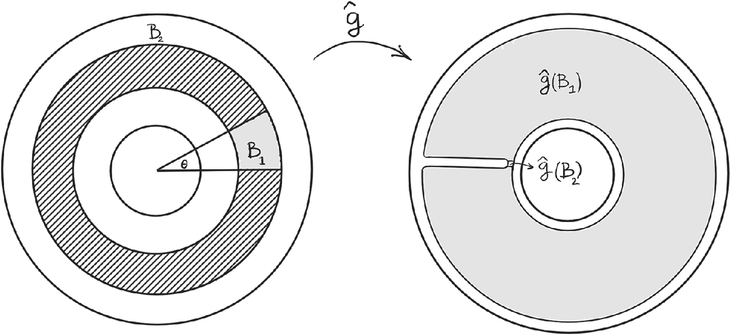
Sublemma. For any
$\sigma < 1$
 close to
$1$
 and
$\epsilon>0$
 small, there is a map
$\hat {g} \in \mathrm {Diff}_{+}^r(\mathbb {A})$
 with the following properties:
-
• $\hat {g}$
is identity on a neighborhood of the set C; -
• $\mathrm{Leb}(\hat {g}(B_{1}))>\sigma $
; -
• $\hat g(B_2)$
is included in the
$\epsilon $
-neighborhood
$N_\epsilon (C)$
of C.Figure 1The map $\hat {g}$
.Figure 1 Long description
The diagram consists of two circular figures connected by a curved arrow labeled g-hat pointing from left to right.
Left Panel:
* A set of four concentric circles.
* At the center, an angle theta is marked within the innermost circle.
* A shaded sector labeled B sub 1 extends from the second circle to the outermost circle within the angle theta.
* A hatched ring labeled B sub 2 occupies the space between the second and third circles, excluding the B sub 1 sector.
Right Panel:
* A large shaded annulus representing the transformation.
* The main shaded area is labeled g-hat (B sub 1).
* A thin, unshaded horizontal slit on the left side leads to a small inner ring labeled g-hat (B sub 2) via a small arrow.


Proof. Using bump functions, we construct a map
$\hat g$
 as depicted in Figure 1. The technical details are left to the reader.
Now, let
$\hat {g}$
 be a map found in the Sublemma. This map can be lifted using the covering map
$\pi :\mathbb {A}\to \mathbb {A}$
 ,
$\pi (r,\theta )=(r,q\theta )$
 . Let g be the lift of
$\hat {g}$
 that is identity around the set C. The diffeomorphism g has similar properties:
-
• ${g}$
is identity on a neighborhood of the set C; -
• $\mathrm{Leb}({g}(\pi ^{-1}(B_{1})))>\sigma $
; -
• ${g}(\pi ^{-1}(B_{2}))\subset N_\epsilon (C)$
.


Now note that g commutes with
$R_{{p}/{q}}$
 , so

Choose
$\alpha '$
 irrational and small enough so that
$h\circ g \circ R_{\alpha '} \circ g^{-1} \circ h^{-1}$
 is arbitrary close to
$h\circ R_{{p}/{q}} \circ h^{-1} $
 . Indeed,
$h\circ g$
 is
$C^r$
 and the map sending
$\alpha $
 to
$h\circ g \circ R_{\alpha } \circ g^{-1} \circ h^{-1}$
 is hence continuous. Since
$\alpha '$
 is irrational, the orbit closure of any point in
$\mathbb {A}$
 under iterating the map
$h\circ g \circ R_{\alpha '} \circ g^{-1} \circ h^{-1}=:f'$
 is an
$h\circ g$
 -image of the orbit closure of a point under iterating the map
$R_{\alpha '}$
 , which is a circle in
$\mathbb {A} $
 . So, for any point
$x\in h\circ g(\pi ^{-1}(B))$
 , the orbit closure of x is the
$h\circ g$
 image of a vertical circle
$C'$
 contained in
$\pi ^{-1}(B)$
 . The map
$h\circ g \circ R_{\alpha '} \circ g^{-1} \circ h^{-1}|_{h\circ g(C')}$
 is conjugate to
$R_{\alpha '}|_{C'}$
 . Now, note that if
$R_{\alpha '}^{n}\circ g^{-1}\circ h^{-1}(x) \in \pi ^{-1}(B_{i})$
 , then
$(f')^{n}(x)\in h\circ g(\pi ^{-1}(B_{i}))$
 for
$i\in \{1,2\}$
 . The orbit of each point in
$C'$
 , on average, spends
${\theta }$
 portion of times in
$\pi ^{-1}(B_1)$
 and
${1-\theta }$
 portion of times in
$\pi ^{-1}(B_2)$
 . So, the orbit of the point x spends
${\theta }$
 portion of times in
$h\circ g(\pi ^{-1}(B_1))$
 and
${1-\theta }$
 portion of times in
$h\circ g(\pi ^{-1}(B_2))$
 . By choosing
$\theta $
 and
$\epsilon $
 sufficiently small, we can guarantee that the asymptotic averages of any point in
$h\circ g(\pi ^{-1}(B_1))$
 is arbitrarily close to a measure
$\nu _{f'}$
 supported on C, which is the pushforward of the Lebesgue measure on the boundary component C by the map
$h\circ g$
 . This is because the image of
$\pi ^{-1}(B_1)$
 under the map g can be so close to C that after iteration by h, it still remains arbitrarily close to C. Since h is smooth and sends positive measure sets to positive measure sets, it can be shown that the sets with large measure are sent to large measure sets. Hence, if
$\sigma $
 is chosen sufficiently close to one, then map g is so that
$\mathrm{Leb}(h\circ g(\pi ^{-1}(B_1)))$
 is sufficiently close to one and so since for a large number n, the nth empirical measures of points in
$h\circ g(\pi ^{-1}(B_1))$
 is close to
$\nu _{h\circ g}$
 , the measure
$\hat {e}^{f'}_n$
 is close to
$\hat {\delta }_{\nu _{f'}}$
 . Now, taking
$\nu $
 as any accumulation point of measures like
$\nu _{f'}$
 , where
$f'$
 approaches f, according to the definition, we can see that f statistically bifurcates toward
$\hat {\delta }_{\nu }$
 and so we are done.
Proof of Theorem A.
Lemma 5.2 implies that for any map
$f\in \mathcal {AK}^r$
 , there are two measures
$\nu _{1,f}$
 and
$\nu _{2,f}$
 that are supported on different connected components of the boundary of
$\mathbb {A}$
 such that f statistically bifurcates toward both
$\hat {\delta }_{\nu _{1,f}}$
 and
$\hat {\delta }_{\nu _{2,f}}$
 . Now, using Theorem B.16, we conclude that for a generic map
$f\in \mathcal {AK}^r$
 and for almost every point x in the phase space X, the set of accumulation points of the sequence
$\{{e}_n^f(x)\}_n$
 contains at least two measures
${\nu _{1,f}}$
 and
${\nu _{2,f}}$
 . We are going to show that, generically, these two measures are the only ergodic invariant measures of the map f and the empirical measures of almost every point accumulate to any convex combination of these two ergodic measures (which is indeed the whole space of invariant measures), and hence, f is maximally oscillating. Now, approximate f by a map like
$h\circ g\circ R_{\alpha '}\circ g^{-1}\circ h^{-1}$
 coming from Lemma 5.2. Using the theorem of Fayad and Katok, we know that the map
$R_{\alpha '}$
 can be approximated in
$C^\infty $
 -topology (and hence in
$C^r$
 -topology) by a map
$e\in \mathcal {AK}_{\mathrm{vol}}^\infty $
 that has only three ergodic measures: two one-dimensional Lebesgue measures on the boundaries and the volume measure of the annulus. The map
$h\circ g\circ e \circ g^{-1} \circ h^{-1}$
 is close to the initial map f and has only three ergodic invariant measures, which are the push forward of three ergodic measures of e by the map
$h\circ g$
 . Note that if in the Sublemma, the numbers
$r_1$
 and
$r_2$
 are chosen close to
$0$
 and
$1$
 , then the set
$B_2$
 has measure close to one. In this case, observe that the pushforward of the volume measure by the map
$h\circ g$
 is a measure that is close to the pushforward of the one-dimensional Lebesgue measure of one of the boundary components (which is denoted by C in the lemma). Hence, the set of invariant measures for the map
$h\circ g\circ e\circ g^{-1}\circ h^{-1}$
 is a triangle that has two of its vertices very close to each other. We know that the map sending the dynamics to its set of invariant measures is upper semi-continuous (see Lemma B.12) and, hence, it is continuous for maps in a Baire generic set. Therefore, we can assume that f is a continuity point of this mapping and the set of invariant measures of f is in an arbitrary neighborhood of a triangle that is arbitrarily close to a segment. So, the set of invariant measures of f is a segment. However, this means that f has exactly two ergodic invariant measures. Note that these measures are supported by different boundary components of the annulus. So, on each boundary component of the annulus, there is only one ergodic measure and, hence, any invariant measures on one of the boundary components are equal to the corresponding ergodic measure on that component. So, f statistically bifurcates toward two measures
$\hat {\delta }_{\nu _{1,f}}$
 and
$\hat {\delta }_{\nu _{2,f}}$
 , and
$\nu _{1,f},\nu _{2,f}$
 are exactly two ergodic measures of f. Moreover, since these two measures are in the accumulation points of the sequence of empirical measures for almost every point and the set of invariant measures is the line segment between these two measures, the sequence of empirical measures of almost every point has to accumulate to every point in this line segment and this finishes the proof.
A Appendix. The
$L^1$
convergence version

We recall the nth empirical function of a map f is the map
$e^f_n:X\to \mathcal M_1(X)$
 sending a point
$x\in X$
 to the nth empirical measure
$e^f_n(x)$
 . We are going to study the
$L^1$
 (non-)convergence of the sequence of empirical functions. For this purpose, we need to give some definitions.
Let us denote the space of Borel measurable maps from X to
$\mathcal M_1(X) $
 by
$L^1(X,\mathcal M_1(X))$
 . Note that since the empirical functions are continuous maps with respect to x, they are elements of
$L^1(X,\mathcal M_1(X))$
 . We define a metric on this space where the distance between two elements
$e,e'\in L^1(X,\mathcal M_1(X))$
 is defined as follows:

Let us study the convergence of the sequence of empirical functions with respect to this metric.
Definition A.1. We say a map f is
$L^1$
 non-statistical if the sequence of maps
$e^f_{n}:X\to \mathcal M_1(X)$
 is not convergent for the
$L^1$
 topology:

In the following, we introduce a condition that if it is satisfied by a Baire space of dynamics
$\Lambda $
 , then we can conclude the existence of
$L^1$
 non-statistical maps within
$\Lambda $
 . Let us first, quantify the extent to which the statistical behavior of a map
$f\in \Lambda $
 can be changed by small perturbations. To this aim, we propose the following definition.
Definition A.2. The amplitude of
$L^1$
 statistical divergence with respect to
$\Lambda $
 of a map
$f\in \Lambda $
 is a real-valued non-negative mapping that is defined as follows:

Note that the definition of
$\Delta ^1$
 depends also on the set
$\Lambda $
 and not only on the map f. However, for the sake of simplicity, we hid this in the notation.
Observe that if
$\Delta ^1$
 is positive at f, then the asymptotic behaviors of dynamics close to f are very sensitive to perturbations and in this sense, the map f is statistically unstable. We introduce the following definition.
Definition A.3. A map
$f\in \Lambda $
 is
$L^1$
 statistically unstable with respect to
$\Lambda $
 if its amplitude of
$L^1$
 statistical divergence with respect to
$\Lambda $
 is positive:

Example A.4. Suppose
$\Lambda $
 is the set of rigid rotations on
$\mathbb {S}^1$
 . The identity map
$\mathrm {Id}_{\mathbb {S}^1}\in \Lambda $
 is
$L^1$
 statistically unstable, since the empirical measures of all of its points are atomic, whereas we can approach the map
$\mathrm {Id}_{\mathbb {S}^1}$
 by irrational rotations and the empirical measures of any point are close to the Lebesgue measure for large enough iterations.
Now, we want to investigate the relationship between
$L^1$
 statistical instability and the existence of
$L^1$
 non-statistical maps. It is clear that if a map f is
$L^1$
 non-statistical, then
$\Delta ^1(f)>0$
 and so f is
$L^1$
 statistically unstable, but the existence of an
$L^1 $
 statistically unstable map does not necessarily imply the existence of
$L^1$
 non-statistical maps (see Example A.4). However, if the interior of
$L^1$
 statistically unstable maps is non-empty, then the existence of plenty of
$L^1$
 non-statistical maps is guaranteed.
Theorem D. The
$L^1$
 non-statistical maps form a Baire generic subset of the interior of
$L^1$
 statistically unstable maps.

The proof of Theorem D uses the following lemma.
Lemma A.6. The map
$\Delta ^1$
 is upper semi-continuous.
Proof. Let
$\{f_k\}_k $
 be a sequence of maps converging to f. For each k, we can find two natural numbers
$n_k$
 and
$m_k$
 , and two maps
$g_k$
 and
$h_k$
 near
$f_k$
 such that

Note that we can choose the sequences
$\{n_k\}_k$
 and
$\{m_k\}_k$
 both converging to infinity and also the sequence of maps
$\{g_k\}_k$
 and
$\{h_k\}_k$
 both converging to f. So, we obtain

and this implies the upper semi-continuity of
$\Delta ^1$
 .
Proof of Theorem D.
Since
$\Delta ^1$
 is upper semi-continuous, there is a generic subset
$\mathcal {G}\subset \Lambda $
 on which the map
$\Delta ^1$
 is continuous. For a map
$f \in \mathcal {G}$
 , which is also in the interior of
$L^1$
 statistically unstable maps, there exists a neighborhood
$\mathcal {U}_f\subset \Lambda $
 around f on which
$\Delta ^1$
 is uniformly positive:

Now, we construct a sequence of open and dense subsets in
${\mathcal U}_f$
 such that any map in the intersections of these sets is
$L^1$
 non-statistical. This will imply that
$L^1$
 non-statistical maps are Baire generic in
${\mathcal U}_f$
 and, hence, the
$L^1$
 non-statistical maps are locally generic in the interior of
$L^1$
 statistically unstable maps.
To construct such open and dense sets, first note that the function
$\Delta ^1$
 can be written as

where
$\Delta ^1_{N}(h,g)=\sup _{i,j\ge N}d_{L^1}(e^h_{i},e^g_{j}).$

Claim. The map
$\Delta ^1_{N}$
 is lower semi-continuous.
Proof. Note that

However,
$\sup _{N \le i,j \le M}d_{L^1}(e^h_{i},e^g_{j})$
 is continuous with respect to
$(h,g)$
 and the supremum of a sequence of continuous functions is lower semi-continuous.
Next, we show that for any
$N\in \mathbb N$
 , the set

is an open and dense subset of
${\mathcal U}_f$
 , and moreover, every map in the intersection
$\bigcap _N E(N)$
 is
$L^1$
 non-statistical.
The openness of
$E(N)$
 is guaranteed by lower semi-continuity of
$\Delta ^1_N.$
 Now, we prove the denseness of
$E(N)$
 . For any arbitrary map
$h\in {\mathcal U}_f$
 , take a neighborhood
$V_h$
 such that for any map
$g\in V_h$
 , we have

This is possible because N is fixed and
$e^g_{N}$
 depends continuously on g. By (A.2), we know that
$\Delta ^1(h)>d$
 and so we can choose
$g_1,g_2 \in V_h$
 such that for some integers
$n,m>N$
 , it holds true that

However, note that

Inequalities (A.3) and (A.4) imply that either

So, at least one of the maps
${g_1}$
 or
${g_2}$
 is inside
$E(N)$
 , and then recalling that h was chosen arbitrarily in
${\mathcal U}_f$
 and
$V_h$
 , we conclude that
$E(N)$
 is dense in
${\mathcal U}_f$
 .
Now, observe that for any map
$h\in \bigcap _{N=1}^\infty E(N)$
 , the sequence of empirical functions is not a Cauchy sequence and, hence, h is
$L^1$
 non-statistical. The set
$\bigcap _{N=1}^\infty E(N)$
 is a Baire generic set in the open neighborhood
$\mathcal U_f$
 , so the
$L^1$
 non-statistical maps are generic in the set
$\mathcal U_f$
 . Considering the fact that f is an arbitrary map in the generic set
$\mathcal G$
 , we can then conclude that
$L^1 $
 non-statistical maps are indeed a generic subset of the interior of
$L^1$
 statistically unstable maps.
B Appendix. The version of convergence in law
For a dynamical system
$f:X\to X$
 , the map
$e^f_n:X\to \mathcal M _1(X)$
 associates to each point
${x\in X}$
 its nth empirical measure. Different points usually have different empirical measures. We can investigate how the empirical measures
$e^f_n(x)$
 are distributed in
$\mathcal M_1(X)$
 with respect to the reference measure
$\mu $
 on X and what is the asymptotic behavior of these distributions. To this aim, we can push forward the measure
$\mu $
 to the set of probability measures on X using the map
$e^f_n$
 :

The measure
$\hat {e}_n(f)$
 is a probability measure on the space of probability measures on X. We denote the space of probability measures on the space of probability measures by
$\mathcal M_1(\mathcal M _1(X))$
 . We denote the Wasserstein metric on this space by
$\hat {d}$
 . Note that the compactness of X implies the compactness of
$\mathcal M_1(X)$
 and, hence, the compactness of
$\mathcal M_1(\mathcal M_1(X))$
 . So, the sequence
$\{\hat {e}_n(f)\}_{n\in \mathbb {N}}$
 lives in a compact space and has one or possibly more than one accumulation points.
Definition B.1. A map f is called statistical in law if the sequence
$\{\hat {e}_n(f)\}_{n\in \mathbb {N}}$
 is convergent.
Example B.2. For any
$\mu $
 -preserving map
$f:X\to X$
 , the sequence
$\{\hat {e}_n(f)\}_{n\in \mathbb {N}}$
 converges to a measure
$\hat {\mu }$
 , which is the ergodic decomposition of the measure
$\mu $
 .
Example B.3. If
$\nu $
 is a physical measure for the map
$f:X\to X$
 whose basin covers
$\mu $
 -almost every point, the sequence
$\{\hat {e}_n(f)\}_{n\in \mathbb {N}}$
 converges to the Dirac mass concentrated on the point
$\mu \in \mathcal M_1(X)$
 , which we denote by
$\hat {\delta }_\mu $
 .
The following lemma provides some information about the sequence
$\{\hat {e}_n(f)\}_{n\in \mathbb {N}}$
 .
Lemma B.4. For any
$f\in \Lambda $
 and any
$n\in \mathbb {N}$
 , it holds true that

where
$\mathrm{diam}(X)$
 is the diameter of the space X.
Proof. We recall that

First, let us show for any
$x\in X$
 the following inequality holds true independent of the choice of
$f\in \Lambda $
 :

So, according to the definition, we should show that

Consider the following element of
$\pi (e^f_n(x),e^f_{n+1}(x))$
 :

Note that


where
$\pi _1$
 and
$\pi _2$
 are the projection on the first and second coordinates. So, we have
${\gamma \in \pi (e^f_n(x),e^f_{n+1}(x))}$
 and, hence,

Now, consider the following measure on
$\mathcal M_1(\mathcal M_1(X))\times \mathcal M_1(\mathcal M_1(X))$
 :

Obviously,
$\hat {\gamma }\in \pi (\hat {e}^f_n,\hat {e}^f_{n+1})$
 , and so

Now, let
$\Lambda $
 be a Baire space of self-mappings of X endowed with a topology finer than
$C^0$
 -topology. For each
$f\in \Lambda $
 , the accumulation points of the sequence
$\{\hat {e}_n(f)\}_{n\in \mathbb {N}}$
 form a compact subset of
$\mathcal M_1(\mathcal M_1(X))$
 , which we denote by
$\mathrm{acc}( \{\hat {e}_n(f)\}_{n\in \mathbb {N}})$
 . This set can vary dramatically by small perturbations of f in
$\Lambda $
 .
For any map
$f\in \Lambda $
 , by
$\mathcal {B}_{\Lambda ,f}$
 , we denote the set of those measures
$\hat {\nu }\in \mathcal M_1(\mathcal M_1(X))$
 that f statistically bifurcates toward
$\hat {\nu }$
 through perturbations in
$\Lambda $
 . Please see Definition 5.1.
Definition B.5. A map
$f\in \Lambda $
 is called statistically unstable in law with respect to
$\Lambda $
 if the set
$B_{\Lambda ,f}$
 has more than one element.
Remark B.6. By definition, it holds true that

Here are some nice properties of the set
$\mathcal {B}_{\Lambda ,f}$
 .
Lemma B.7. The set
$\mathcal {B}_{\Lambda ,f}$
 is a compact subset of
$\mathcal M_1(\mathcal M_1(X))$
 .
Proof. By the definition, it is clear that the set
$\mathcal {B}_{\Lambda ,f}$
 is closed. The compactness is a consequence of the compactness of
$\mathcal M_1(\mathcal M_1(X))$
 .
Lemma B.8. The set
$\mathcal {B}_{\Lambda ,f}$
 is a connected subset of
$\mathcal M_1(\mathcal M_1(X))$
 .
Proof. For the sake of the contrary, assume that
$B_{\Lambda ,f}$
 is not connected, and can be decomposed to two non-empty disjoint closed sets A and B. Therefore, there is some real number
$d>0$
 such that
$\tilde {d}_w(A,B)>d.$
 Take two elements
$\hat {\nu }\in A$
 and
$\hat {\eta }\in B$
 and let N in Lemma B.4 be chosen so that

We can find a neighborhood U of f so that

This is possible since the map sending f to
$\hat {e}_N^f $
 is continuous. Now, take two maps
$h,g\in U$
 such that for some integers
$n_1,n_2>N$
 , it holds true that

Consider the following sequence of elements of
$\mathcal M_1(\mathcal M_1(X))$
 :

The distance between two consecutive elements of this sequence is less than
${d}/{3}$
 and, hence, there is an element of this sequence that lies out of the
${d}/{3}$
 neighborhood of
$A\cup B=B_{\Lambda ,f}$
 . By taking N larger, we obtain another element of
$\mathcal M_1(\mathcal M_1(X))$
 out of the
${d}/{3}$
 neighborhood of
$B_{\Lambda ,f}$
 . So, there is a sequence like
$\hat {e}_{n_k}^{f_k}$
 out of the
${d}/{3}$
 neighborhood of
$B_{\Lambda ,f}$
 and because of the compactness of
$\mathcal M_1(\mathcal M_1(X))$
 , this sequence has a convergent subsequence converging to an element out of
$B_{\Lambda ,f}$
 . By definition, any accumulation point of this sequence is an element of
$B_{\Lambda ,f}$
 , which is a contradiction.
Lemma B.9. For any
$\hat {\nu }\in \mathcal B_{\Lambda ,f}$
 , any measure
$\nu $
 in the support of
$\hat {\nu }$
 is invariant under iteration of f.
Proof. By definition, there is a sequence of maps
$\{f_k\}_k$
 in
$\Lambda $
 converging to f and a sequence of natural numbers
$\{n_k\}_k$
 converging to infinity such that

If
$\nu $
 is in the support of
$ \hat {\nu }$
 , then for any neighborhood
$\mathcal U$
 of
$\nu $
 and for k large enough, we have

Recalling that

we conclude that the integrand of the integral above is non-zero for a subset of X with positive measure and, hence, in particular for each k, there is a point
$x_k\in X$
 such that
$e^{f_k}_{n_k}(x_k)\in \mathcal U$
 . Since
$\mathcal U $
 is an arbitrary neighborhood of
$\nu $
 , we can choose
$x_k$
 such that

However, note that for a large k, the map
$f_k$
 is close to the map f so the measure
$e^{f_k}_{n_k}(x_k)$
 is close to
$f_*(e^{f_k}_{n_k}(x_k)$
 . So, we have

which, together with the continuity of
$f_*$
 , implies that
$f_*(\nu )=\nu $
 and so we are done.
The set
$\mathcal B_{\Lambda ,f}$
 depends on the choice of the set of dynamics
$\Lambda $
 in which we are allowed to perturb the map f. If
$\Lambda $
 is replaced by a larger set of maps, then we may have more elements in
$\mathcal M_1(\mathcal M_1(X))$
 toward which f statistically bifurcates. In this appendix, we will show the following theorem.
Theorem E. Suppose X is a compact metric space, endowed with a reference probability measure
$\mu $
 , and
$\Lambda $
 is a set of continuous self-mappings of X, endowed with a topology finer than
$C^0$
 topology. Then, for Baire generic maps
$f\in \Lambda $
 , we have

We will prove this theorem later. Let us recall some definitions that we need in the rest of this section. Let X and Y be two topological spaces with Y compact. Denote the set of all compact subsets of Y by
$C(Y)$
 .
Definition B.11. A map
$\phi :X\to C(Y)$
 is called lower semi-continuous if for any
$x\in X$
 and any V open subset of Y with
$\phi (x)\cap V\neq \emptyset $
 , there is a neighborhood U of x such that for any
$y\in U$
 , the intersection
$\phi (y)\cap V$
 is non-empty. The map
$\phi $
 is called upper semi-continuous if, for any
$x\in X$
 and any V open subset of Y with
$\phi (x)\subset V$
 , there is a neighborhood U of x such that for any
$y\in U$
 , the set
$\phi (y)$
 is contained in V. Finally,
$\phi $
 is called continuous at x if it is both upper and lower semi-continuous at x.
We also recall the following theorem of Fort [Reference Fort22] which generalizes the well-known theorem about real-valued semi-continuous maps to the set-valued semi-continuous maps.
Theorem (Fort).
For any Baire topological space X and compact topological space Y, the set of continuity points of a semi-continuous map from X to
$C(Y)$
 is a Baire generic subset of X.
We recall the following fact on the semi-continuity property of the map sending the dynamics to its set of invariant probability measures.
Lemma B.12. The map sending
$f\in \Lambda $
 to its set of invariant probability measures is upper semi-continuous.
We recall that by Lemma B.7, the set
$\mathcal B_{\Lambda ,f}$
 is compact. We can ask about the dependence of the set
$\mathcal B_{\Lambda ,f}$
 on the map f. The following lemma shows that this dependency is semi-continuous.
Lemma B.13. The map sending
$f\in \Lambda $
 to the set
$\mathcal B_{\Lambda , f}$
 is upper semi-continuous.
For the proof, see [Reference Talebi41, Lemma 1.10].
To each map,
$f\in \Lambda $
 , one can associate the set of accumulation points of the sequence
$\{\hat {e}_n(f)\}_{n\in \mathbb {N}}$
 , which is a compact subset of
$\mathcal M_1 (\mathcal M _1(X))$
 . This map is neither upper semi-continuous nor lower semi-continuous. However, if we add the points of this sequence to its accumulation points and consider the map sending
$f\in \Lambda $
 to the closure
$\overline {\{\hat {e}_n(f) \mid n\in \mathbb {N}\}}$
 , we obtain a semi-continuous map.
Lemma B.14. The map
$\mathcal E: \Lambda \to C({\mathcal M_1(\mathcal M_1(X))})$
 defined as

is lower semi-continuous.
For the proof, see [Reference Talebi41, Lemma 1.11].
The following lemma is an interesting consequence of Lemma B.14 that shows how the set
$\mathcal {E}(f)$
 depends on the dynamics f.
Lemma B.15. A Baire generic map
$f\in \Lambda $
 is a continuity point for the map
$\mathcal E$
 .
This lemma gives a view to the statistical behaviors of generic maps in any Baire space of dynamics: for a generic map, the statistical behavior that can be observed for times close to infinity cannot be changed dramatically by small perturbations.
Proof. Using Lemma B.14, this is a direct consequence of Fort’s theorem.
Now, we are ready to prove Theorem E. This theorem reveals how two notions of statistical instability in law and non-statistical maps in law are connected. There is another proof of this theorem which is communicated by Pierre Berger that can be found in [Reference Talebi41, Theorem 1.14].
Proof of Theorem E.
Take a generic map f from the main lemma above. By Remark B.6,
$\mathrm{acc}(\{\hat {e}_n^f\}_n)\subset B_{\Lambda ,f}$
 . So, if
$B_{\Lambda ,f}$
 has only one element, since
$\mathrm{acc}(\{\hat {e}_n^f\}_n)$
 is non-empty, the equality holds. Now, suppose that
$B_{\Lambda ,f}$
 has more than one element. For the sake of contradiction, suppose there is a measure
$\hat {\nu }\in B_{\Lambda ,f}$
 that is not in
$\mathrm{acc}(\{\hat {e}_n^f\}_n)$
 . Then, there is a number
$n\in \mathbb {N}$
 such that
$\hat {\nu }=\hat {e}_n^f$
 and
$\hat {e}_n^f$
 is an isolated point of the sequence
$\{\hat {e}_n^f\}_n$
 . Recalling that for generic f we have
$B_{\Lambda ,f}\subset \mathcal {E}(f)$
 , we can conclude that
$B_{\Lambda ,f}$
 can be written as a union of two disjoint and non-empty closed sets:

This is contrary to the connectedness of the set
$B_{\Lambda ,f}$
 .
Consider all invariant measures
$\nu $
 that the map f statistically bifurcates toward
$\hat {\delta }_nu$
 . We denote these measures by
$\mathcal M_{\Lambda ,f}$
 , which are defined more precisely as

Theorem B.16. Let
$\Lambda $
 be a Baire space of self-mappings of X endowed with a topology finer than
$C^0$
 -topology. For a Baire generic map
$f\in \Lambda $
 , the empirical measures of
$\mu $
 almost every point
$x\in X$
 , accumulate to each measure in
$\mathcal M _{\Lambda ,f}$
 , or in other words,

For the proof, see [Reference Talebi41, Theorem 1.16].
If one can find any information about the set
$\mathcal M_{\Lambda ,f}$
 for a generic map f in
$\Lambda $
 , then by Theorem B.16, we can translate this information to information about the statistical behavior of
$\mu $
 -almost every point for a generic subset of maps.
The following lemma shows how the set
$\mathcal M_{\Lambda ,f}$
 depends on the map f.
Lemma B.17. The map sending
$f\in \Lambda $
 to the set
$\mathcal M_{\Lambda , f}$
 is upper semi-continuous.
For the proof, see [Reference Talebi41, Lemma 1.16].
Now, let us see what is the consequence of this lemma and Theorem B.16 when we know the maps in a dense subset bifurcate toward each Dirac mass at an invariant measure.
Proposition B.18. (Maximal oscillation)
If there is
$D\subset \Lambda $
 dense such that any map
$f\in D$
 bifurcates toward the Dirac mass at each invariant measure through perturbations in
$\Lambda $
 , or in other words,
$M_{\Lambda ,f}=\mathcal M_1(f)$
 , then a generic
$f\in \Lambda $
 has maximal oscillation.
For the proof, see [Reference Talebi41, Proposition 1.19].
C Appendix. Comparison between different versions
In this section, we compare different versions of defining statistical instability and non-statistical dynamics and show how they are related. The first proposition describes the relation between different versions of defining non-statistical maps.
Proposition C.1. Suppose
$f:X\to X$
 is a continuous map of a compact metric space.
-
(i) If f is non-statistical in law, then it is $L^1$
non-statistical. -
(ii) If f is $L^1$
non-statistical, then it is non-statistical.


Proof. (i) Let f be non-statistical in law. So by definition, the sequence
$\{\hat {e}_n(f)=(e^f_n)_* \mu \}_n$
 is not convergent. We recall that

where
$\hat {\delta }_{e^f_n(x)}\in \mathcal {M}_1(\mathcal {M}_1(X))$
 is the Dirac mass supported on the point
$e^f_n(x)\in \mathcal {M}_1(X)$
 .
Suppose to the contrary that f is not
$L^1$
 non-statistical. So, the sequence of maps
$\{e_n^f:X\to \mathcal {M}_1(X)\}$
 is convergent in the
$L^1$
 topology. Let us call the limit point of this sequence by
$e^f_\infty $
 . Now, we show that
$(e^f_n)_*\mu $
 converges to
$(e^f_\infty )_*\mu $
 , which is a contradiction. For simplicity, we denote
$(e_n^f)_*\mu $
 by
$\nu _n$
 and
$(e_\infty ^f)_*\mu $
 by
$\nu _\infty $
 . We recall that

where
$\pi (\nu _n,\nu _\infty )$
 is the set of all probability measures on
$\mathcal {M}_1(X)\times \mathcal {M}_1(X)$
 that projects to
$\nu _n$
 and
$\nu _\infty $
 under the projections to the first and second coordinate, respectively. Consider the following element of
$\xi_n$
 :

We have

However,

So, we obtain
$\hat {d}_w(\nu _n,\nu _\infty )\leqslant d_{L^1}(e_n^f,e_\infty ^f)$
 , which implies that
$\nu _n$
 is converging to
$\nu _\infty $
 and is a contradiction.
(ii) Let f be
$L^1$
 non-statistical. We show that f is non-statistical and so the maps
$e_n^f:X\to \mathcal {M}_1(X)$
 do not converge almost surely. By contrast, suppose the maps
$e_n^f:X\to \mathcal {M}_1(X)$
 converge almost surely to a map
$e_\infty ^f:X\to \mathcal {M}_1(X)$
 . Hence, the map
$d_w(e_n^f(.), e_\infty ^f(.)):X\to \mathbb {R}$
 converges to zero almost surely and by dominated convergence theorem, we obtain that

which is a contradiction.
We would like to announce here the existence of examples of maps that are
$L^1$
 statistical but non-statistical and the maps that are statistical in law but
$L^1$
 non-statistical. These examples could be constructed on
$\mathbb S^1\times \mathbb A$
 , where
$\mathbb A$
 is the closed annulus, using the Anosov–Katok method and similar ideas described in §5.
The next proposition shows that the same hierarchy holds for different versions of defining statistically unstable maps.
Proposition C.2. Suppose
$\Lambda $
 is a set of continuous self-mappings of a compact metric space X. The following hold true.
-
(i) If $f\in \Lambda $
is statistically unstable in law, then it is
$L^1$
statistically unstable. -
(ii) If $f\in \Lambda $
is
$L^1$
statistically unstable, then it is statistically unstable.


Proof. (i) If f is statistically unstable in law, then by definition, there are at least two different elements
$\hat {\nu }_1$
 and
$\hat {\nu }_2$
 in
$\mathcal {M}_1(\mathcal {M}_1(X))$
 toward which f statistically bifurcates. This means that there are two sequences of maps
$\{f^1_k\}_k$
 and
$\{f^2_k\}_k$
 converging to f, and two sequences of positive integers
$\{n^1_k\}_k$
 and
$\{n^2_k\}_k$
 converging to infinity such that

Now, in contrast, suppose f is
$L^1$
 statistically stable. So, the sequences
$\{e^{f^1_k}_{n^1_k}:X\to M_1(X)\}_k$
 and
$\{e^{f^2_k}_{n^2_k}:X\to M_1(X)\}_k$
 both converge to a map
$e^f_\infty :X\to M_1(X)$
 in the
$L^1$
 topology. Using the same arguments in the proof of part (i) in the previous proposition, we conclude that both sequences
$\{(e^{f^1_k}_{n^1_k})_* \mu \}_k$
 and
$\{(e^{f^2_k}_{n^2_k})_* \mu \}_k$
 converge to
$(e_\infty ^f)_*\mu $
 . Hence, we have
$\hat {\nu }_1=\hat {\nu }_2=(e_\infty ^f)_*\mu $
 , and since
$\hat {\nu }_1$
 and
$\hat {\nu }_2$
 were distinct elements
$\mathcal {M}_1(\mathcal {M}_1(X))$
 , this is a contradiction.
(ii) Suppose f is not statistically stable, so there is a map
$e_\infty ^f:X\to \mathcal {M}_1(X)$
 such that for any sequence
$\{f_k\}_k$
 converging to f and any sequence of natural numbers
$\{n_k\}_k$
 converging to infinity, the sequence of maps
$\{e_{n_k}^{f_k}:X\to \mathcal {M}_1(X)\}_k$
 converge almost surely to the map
$e_\infty ^f$
 . Using the dominated convergence theorem, we conclude the convergence of this sequence in the
$L^1$
 topology to the map
$e_\infty ^f$
 and, hence, f cannot be
$L^1$
 statistically unstable.
Acknowledgments
I would like to express my special thanks to Pierre Berger and Meysam Nassiri for their constant support, and numerous comments and discussions while undertaking this work. I acknowledge Bassam Fayad who gave the idea of improving our result from the Baire genericity of non-statistical Anosov–Katok maps to the Baire genericity of maximally oscillating Anosov–Katok maps. I would like to list all of my financial sources while writing this paper: The Institute for Research in Fundamental Sciences (IPM), Campus France, Iranian Ministry of Science, Research and Technology, and Université Paris 13. This research was in part supported by a grant from IPM (no. 1404370115) and ERC project 818737 Emergence of wild differentiable dynamical systems, and INSF grant no. 4001845.