2 Compositional models and partial contestation

Vote shares are inherently compositional data. If $v_{ij}$ represents party j’s vote share ( $j=1,2\dots ,J$ ) in electoral district i ( $i=1,2\dots ,N$ ), it follows that

(1) $$ \begin{align} 0\leq v_{ij}\leq1 \text{ }\forall j \text{ and } \sum_{j=1}^J v_{ij} = 1. \end{align} $$

To estimate models with vote shares as the outcome, $v_{ij}$ terms can be expressed as $J-1$ log-ratios to unbind them from a 0–1 scale to the real number line (Aitchison Reference Aitchison1982). The denominator of each log-ratio is the vote share of an arbitrarily chosen baseline party ( $j=1$ ) and each numerator is $v_{ij}$ of one of the remaining $J-1$ partiesFootnote ¹ :

(2) $$ \begin{align} s_{ij} = \text{log}\left(\frac{v_{ij}}{v_{i1}}\right) \text{ } \forall \text{ } j \neq 1. \end{align} $$

Katz and King (Reference Katz and King1999) introduced an additive logistic-t model to the study of election outcomes defined as $s_{ij}$ . Tomz, Tucker, and Wittenberg (TTW; Reference Tomz, Tucker and Wittenberg2002) proposed a simpler approach in which they estimated the impact of predictors $\mathbf {x}_{ij}$ on $s_{ij}$ using seemingly unrelated regressions (SURs; Zellner Reference Zellner1962). Estimated coefficients from the SUR equations, $\boldsymbol {\hat {\beta }}_j$ , can be used for inferential hypothesis tests and to calculate quantities of interest such as predicted vote shares, $\hat {v}_{ij}$ . The predictions ( $\hat {s}_{ij}$ ) are translated back into $\hat {v}_{ij}$ using a multivariate logistic transformation (Philips, Rutherford, and Whitten Reference Philips, Rutherford and Whitten2016):

(3) $$ \begin{align} \begin{aligned} \hat{v}_{ij} &= \frac{\exp(\mathbf{x}_{ij}^{\prime}\boldsymbol{\hat{\beta}}_j)}{1+\sum_{j=2}^J \exp(\mathbf{x}_{ij}^{\prime}\boldsymbol{\hat{\beta}}_j)} \text{ } \forall \text{ } j \neq 1,\\ \hat{v}_{i1} &= \frac{1}{1+\sum_{j=2}^J\exp(\mathbf{x}_{ij}^{\prime}\boldsymbol{\hat{\beta}}_j)}. \end{aligned} \end{align} $$

A straightforward solution to modeling vote shares as compositional outcomes has thus been available for over two decades. Despite this, scholars seldom estimate compositional models to study elections (Kagalwala, Moreira, and Whitten Reference Kagalwala, Moreira and Whitten2024a). Even though most theories involve trade-offs across specific parties or ideological families of parties, the dominant approach is to analyze variation in the vote share of one party, typically the incumbent, against all other categories at the national or district level (e.g., Cavallaro, Pregliasco, and Vassallo Reference Cavallaro, Pregliasco and Vassallo2018; Colantone and Stanig Reference Colantone and Stanig2018; Duch and Stevenson Reference Duch and Stevenson2005; Kayser and Peress Reference Kayser and Peress2012; Powell Jr. and Whitten Reference Powell and Whitten1993; Ward Reference Ward2020). The most common explanation offered for why scholars choose not to model election results as compositions is the presence of partial contestation.

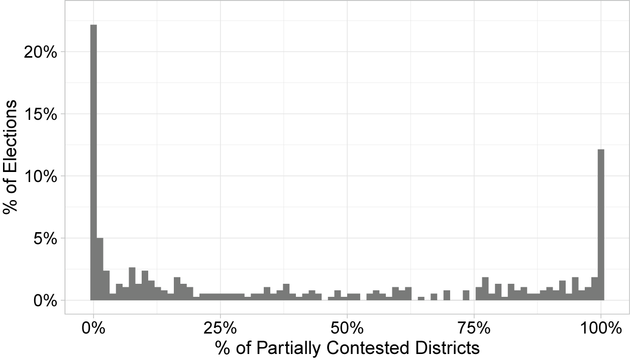
In Figure 1, we show that partial contestation is a common occurrence around the world.Footnote ² In a sample of 377 national elections across 63 countries between 1970 and 2019, in only 80 elections (21.1%), all parties contested all districts. More than 50% of districts were partially contested in 40.1% of all cases (152 elections).Footnote ³

Figure 1

Contestation in 377 elections across 63 countries (1970–2019).

Note: Constituency-Level Elections Archive (CLEA).

Figure 1. Long description

The X-axis is labeled % of Partially Contested Districts with major ticks at 0%, 25%, 50%, 75%, and 100%. The Y-axis is labeled % of Elections with major ticks at 0%, 5%, 10%, 15%, and 20%.

* The distribution is U-shaped, indicating that most elections either have very few or almost all districts partially contested.

* The highest peak is at the 0% mark on the X-axis, where the percentage of elections exceeds 20%.

* A second significant peak occurs at the 100% mark on the X-axis, reaching approximately 12% of elections.

* Between 5% and 95% on the X-axis, the frequency of elections remains low and relatively flat, generally fluctuating between 0% and 3%.

Partial contestation creates two major problems. First, the categories of the compositional outcome vary across districts.Footnote ⁴ Second, partial contestation is an example of sample selection. To address the first issue, Katz and King recommended estimating the “effective vote”: $v_{ij}$ we would observe if all J parties had a candidate in all N districts (Reference Katz and King1999, 22). But as TTW noted, this insertion of a party into a race “awards that party more votes than it actually earned, at the expense of parties that truly competed” in that district (Reference Tomz, Tucker and Wittenberg2002, 69). Instead, they proposed estimating separate SUR models for each pattern of contestation, a cumbersome strategy that can become unfeasible and leads to inconclusive analyses as the number of patterns of contestation increases and when there are few districts with a particular pattern of contestation. Kagalwala et al. (Reference Kagalwala, Moreira and Whitten2024a) showed that researchers do not follow this approach; rather, when using compositional models to study elections, they employed some form of data modification to address partial contestation. The most common strategy used in political science is to limit the sample to fully contested districts.

Other strategies to get around partial contestation also involve data modification. Pattie and Johnston (Reference Pattie and Johnston2009), for instance, replaced missing $v_{ij}$ terms for parties that did not contest a district with a tiny value, 0.001 (0.1%), of the votes in the district:

(4) $$ \begin{align} s^{*}_{ij} = \begin{cases} \text{log}\left(\frac{v_{ij}+0.001}{v_{i1}}\right) & \text{if } v_{ij} = 0 \\ s_{ij} & \text{if } v_{ij}> 0. \end{cases} \end{align} $$

This small adjustment avoids zero values in Equation (2) that transforms $v_{ij}$ into log ratios. The authors then use the SUR approach to estimate a single system of equations across all districts. However, this “tiny value” strategy “results in biased estimates, and the magnitude of the bias increases with the share of partially contested districts” (Kagalwala et al. Reference Kagalwala, Moreira and Whitten2024a, 7). This happens because the data adjustment in Equation (4) attenuates the relationship between a predictor of interest and $s_{ij}$ . To address this, for each party that did not contest every district, Kagalwala et al. (Reference Kagalwala, Moreira and Whitten2024a) included a dummy variable indicating whether party j contested district i. The dummy variable for j is then interacted with other predictors in j’s log-ratio equation in the SUR. This “dummy variable” approach is equivalent to estimating an SUR model with only fully contested districts and avoids the pitfalls of the TTW strategy created by data limitations such as small samples when many constituencies are partially contested. However, this relatively simple strategy does not address the second problem that stems from partially contested elections: sample selection.

3 Accounting for sample selection in compositional data

Political parties do not randomly select the districts where they field candidates. Parties are collective entities seeking to maximize their chances of winning legislative seats while constrained by a finite amount of campaign resources (Boix Reference Boix, Boix and Stokes2009). Unobservable factors influencing their decision of where to compete are likely correlated with the party’s expected performance. For example, a party’s reputation and the quality of its candidate in a district should affect both its decision to contest the district and the vote share it receives when it does contest that district (e.g., Butler and Powell Reference Butler and Powell2014; Cox and Katz Reference Cox and Katz1996). This is a classic sample selection problem and failing to account for it results in biased parameter estimates (Heckman Reference Heckman1976, Reference Heckman1979). Heckman (Reference Heckman1979) showed that such situations are analogous to an omitted variable problem and can be addressed using a two-stage estimator with selection and outcome equations.

In elections, the first stage models the likelihood that party j will contest district i, and we only observe $v_{ij}$ if j chooses to contest i. This selection mechanism can be defined as

(5) $$ \begin{align} d_{ij}^* = \mathbf{z}_{ij}^{\prime}\boldsymbol{\alpha}_j + \varepsilon_{ij}, \end{align} $$

where $d_{ij}^*$ is the latent utility of j contesting i, $\mathbf {z}_{ij}$ is a vector of predictors and $\varepsilon _{ij}$ is the random error. Then, the selection stage we observe is

$$ \begin{align*} d_{ij} = \begin{cases} 1 & \text{if } d_{ij}^* \geq 0 \\ 0 & \text{if } d_{ij}^* < 0. \end{cases} \end{align*} $$

Using a single-outcome equation as a general case, the second stage consists of predictors that affect j’s electoral performance in a given i. Let this outcome be

(6) $$ \begin{align} v_{ij} = \mathbf{x}_{ij}^{\prime}\boldsymbol{\beta}_{j}+u_{ij}, \end{align} $$

where $v_{ij}$ is observed if $d_{ij}=1$ and is otherwise missing. Heckman (Reference Heckman1979) showed that failing to account for sample selection in Equation (6) leads to biased estimates ( $\boldsymbol {\hat {\beta }}_{j}$ ). His two-step solution is:

1. 1. Estimate Equation (5) with a probit model.

2. 2. Estimate Equation (6) with OLS controlling for the inverse Mills ratio, $\frac {\phi (\mathbf {z}^{\prime }_{ij}\hat {\alpha }_j)}{\Phi (\mathbf {z}^{\prime }_{ij}\hat {\alpha }_j)}$ , evaluated at the set of observables that influence the selection stage.

This strategy, known as “Heckman correction,” uses the inverse Mills ratio from the first stage to correct for sample selection in the second stage. This approach relies on two assumptions for identification: the error terms in both stages are bivariate normally distributed, and there is a valid exclusion restriction—that is, at least one explanatory variable in the selection equation is excluded from the outcome stage (Achen Reference Achen1986; Cook et al. Reference Cook, Lee and Newberger2021; Sartori Reference Sartori2003; Wolfolds and Siegel Reference Wolfolds and Siegel2019). Therefore, there must exist one variable in $\mathbf {z}_{ij}$ influencing $d_{ij}^*$ that does not affect $v_{ij}$ . When this exclusion restriction is violated, Heckman estimators are identified solely from distributional assumptions about the residuals, and the estimation procedure works “poorly in practice due to near collinearity” (Achen Reference Achen1986, 99).Footnote ⁵

The Heckman correction is inappropriate for compositional models derived from discrete choices (e.g., vote choices when parties partially contest districts) because they typically violate the assumption of normally distributed errors. Instead of a single outcome equation, the compositional nature of elections implies that the outcome stage isFootnote ⁶

(7) $$ \begin{align} v_{ij} = \begin{cases} \frac{\exp(s_{ij})}{1 + \sum^{J}_{j=2}(\exp(s_{ij}))} \text{ }\forall j \neq 1 & \text{if } d_{ij} = 1 \\ \text{missing} & \text{if } d_{ij} = 0. \end{cases} \end{align} $$

The log-transformation in Equation (2) imposes that the error terms in log-ratio equations are Gumbel distributed (Aitchison Reference Aitchison1982; Train Reference Train2009).Footnote ⁷ The monotonic transformations of $v_{ij}$ terms change the distribution of the random component (McFadden Reference McFadden and Zarembka1974, 111). This is similar to assumptions about error terms commonly made with multinomial logistic models: the stochastic components are independently and identically Gumbel distributed (Train Reference Train2009, 34).Footnote ⁸ Thus, accounting for sample selection by treating $u_{ij}$ and $\varepsilon _{ij}$ as jointly normal and using the inverse Mills ratio is no longer an adequate strategy. This will result in inefficiency and, without a valid instrument, in severe bias (Newey, Powell, and Walker Reference Newey, Powell and Walker1990; Sartori Reference Sartori2003; Wolfolds and Siegel Reference Wolfolds and Siegel2019).

To overcome this issue, we propose an MLE approach that accounts for sample selection in a compositional framework derived from a multinomial discrete choice process.Footnote ⁹ The conditional expectation of observing $v_{ij}$ in Equation (7) is

(8) $$ \begin{align} \mathbb{E}[s_{ij} | \mathbf{x}^{\prime}_{ij}, d_{ij} =1] = \mathbf{x}^{\prime}_{ij}\boldsymbol{\beta}_j + \mathbb{E}[u_{ij}|\varepsilon_{ij} \geq -\mathbf{z}^{\prime}_{ij}\boldsymbol{\alpha}_{j}], \end{align} $$

where $\mathbb {E}[u_{ij}|\varepsilon _{ij} \geq -\mathbf {z}^{\prime }_{ij}\boldsymbol {\alpha }_{j}] \neq 0$ .Footnote ¹⁰ If $u_{ij}$ and $\varepsilon _{ij}$ were jointly normal, then adding the inverse Mills ratio to the right-hand side of outcome equations could result in consistent parameter estimates (Heckman Reference Heckman1979). However, since compositional outcomes are transformed to log ratios, $u_{ij}$ and $\varepsilon _{ij}$ are assumed to follow a bivariate Gumbel distribution. Their marginal distributions are (Train Reference Train2009, 34)

(9) $$ \begin{align} f(w) = e^{-(w+\gamma+e^{-(w+\gamma)})}, \end{align} $$

where $\gamma $ is the Euler–Mascheroni constant. We can then estimate both stages simultaneously with the following likelihood function:

(10) $$ \begin{align} \mathcal{L}_j = \prod_{i=1}^N \mathbb{P}(\varepsilon_{ij}> -\mathbf{z}^{\prime}_{ij}\boldsymbol{\alpha}_{j})^{d_{ij}} f_{u|\varepsilon}(s_{ij} - \mathbf{x}^{\prime}_{ij}\boldsymbol{\beta}_{j}|\varepsilon_{ij} > -\mathbf{z}^{\prime}_{ij}\boldsymbol{\alpha}_{j})^{d_{ij}} \mathbb{P}(\varepsilon_{ij} < -\mathbf{z}^{\prime}_{ij}\boldsymbol{\alpha}_{j})^{1-d_{ij}}, \end{align} $$

where $\mathbb {P}(\varepsilon _{ij}> -\mathbf {z}^{\prime }_{ij}\boldsymbol {\alpha }_{j})^{d_{ij}}$ 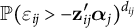is the likelihood that j competes in district i, $f_{u|\varepsilon }(s_{ij}-\mathbf {x}^{\prime }_{ij}\boldsymbol {\beta }_{j}|\varepsilon _{ij}> -\mathbf {z}^{\prime }_{ij}\boldsymbol {\alpha }_{j})^{d_{ij}}$ is the likelihood of observing $v_{ji}$ given that j contested i and $\mathbb {P}(\varepsilon _{ij} < -\mathbf {z}^{\prime }_{ij}\boldsymbol {\alpha }_{j})^{1-d_{ij}}$ is the likelihood that j does not contest i. The log-likelihood is thenFootnote ¹¹

(11) $$ \begin{align} \text{log}(\mathcal{L}_j) = \sum_{i=1}^N d_{ij} \text{log} \bigg( \int_{-\mathbf{z}^{\prime}_{ij}\boldsymbol{\alpha}_{j}}^{\infty} f_{u\varepsilon}(s_{ij} - \mathbf{x}^{\prime}_{ij}\boldsymbol{\beta}_{j},\ \varepsilon_{ij})\textrm{d}\varepsilon_{ij} \bigg) + \sum_{i=1}^N (1-d_{ij}) \text{log}(F_\varepsilon(-\mathbf{z}^{\prime}_{ij}\boldsymbol{\alpha}_{j})), \end{align} $$

where $F_\varepsilon $ is $\varepsilon _{ij}$ ’s marginal CDF and $f_{u\varepsilon }$ is the joint density of $u_{ij}$ and $\varepsilon _{ij}$ . The CDF and PDF of the jointly Gumbel distributed $u_{ij}$ and $\epsilon _{ij}$ are, respectively,

(12) $$ \begin{align} &F(u,\ \varepsilon; m) = \exp\bigg[-(e^{-mu} + e^{-m\varepsilon})^{\frac{1}{m}}\bigg] \end{align} $$

(13) $$ \begin{align} &f(u, \varepsilon; m) = f_{u\varepsilon} = F(u, \varepsilon; m)e^{-m(u+\varepsilon)}(e^{-mu} + e^{-m\varepsilon})^{\frac{1}{m}-2}.\bigg[m-1+(e^{-mu} + e^{-m\varepsilon})^{\frac{1}{m}}\bigg], \end{align} $$

where $m = \frac {1}{1-\rho }\in [1, \infty ]$ 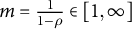, $\rho $ is the correlation between $u_{ij}$ and $\varepsilon _{ij}$ , and $m=1$ when $u_{ij}$ and $\varepsilon _{ij}$ are independently distributed.Footnote ¹² This approach (CMS) allows scholars to fully test hypotheses about trade-offs across parties while correcting for sample selection arising from strategic partial contestation.Footnote ¹³

4 Simulations: Sample selection in compositional outcomes

To evaluate the efficacy of our proposed approach, we conduct a series of Monte Carlo experiments. We compare our CMS with the following four alternatives:

1. 1. Heckman correction: Including an inverse Mills ratio for parties that partially contest electoral districts on the right-hand side of their respective log-ratio equations.

2. 2. TTW: Estimating an SUR model for only fully contested districts. Although TTW (Reference Tomz, Tucker and Wittenberg2002) recommended estimating a separate SUR model for each pattern of contestation, restricting the sample to fully contested districts is the most common implementation of their strategy.

3. 3. Tiny value: Adding a tiny value (0.01%) for parties that do not contest in a district and estimating SUR models.

4. 4. Tiny value with dummy variables: Imputing a tiny value (0.01%) for parties that do not contest in a district and accounting for partial contestation by including dummy variables for parties that partially contest districts and interacting these with other predictors (Kagalwala et al. Reference Kagalwala, Moreira and Whitten2024a).

Our data-generating process (DGP) includes three parties $j \in \{A, B, C\}$ contesting elections in N districts ( $i=1,\dots ,N$ ).Footnote ¹⁴ B and C contest all N districts, and A fields candidates only in some districts. A’s contestation is determined by the following equation:

(14) $$ \begin{align} d^*_{iA} = \alpha_{0A} + \alpha_{1A}z_{1i} + \alpha_{2A} z_{2i} + \varepsilon_{iA}, \end{align} $$

where A contests i if $d^*_{iA} \geq 0$ . We vary $\alpha _{0A}$ depending on partially contested districts such that ${\alpha _{0A}=}$  0.57, 0, or $-0.53$ when A contests 33%, 50%, or 66% of districts, respectively. $\alpha _{1A}=0.8$ and $\alpha _{2A}=0.2$ . C is the baseline category in the compositional outcomes:

(15) $$ \begin{align} s_{ij} = \text{log}\left(\frac{v_{ij}}{v_{iC}}\right) = \beta_{0j} + \beta_{1j}z_{1i} + \beta_{2j}z_{2i} + u_{ij}, \end{align} $$

where $\beta _{0A}=1$ , $\beta _{1A}=1.2$ , $\beta _{0B}=1$ , $\beta _{1B}=-1$ and $\beta _{2A}=\beta _{2B}=0$ for our initial set of experiments. Additionally, $u_{iA}$ and $\varepsilon _{iA}$ are jointly generated from mean-zero extreme value type-I distributions (McFadden Reference McFadden and Zarembka1974; Train Reference Train2009).Footnote ¹⁵ As per Heckman (Reference Heckman1979), failing to account for the correlation between $u_{iA}$ and $\varepsilon _{iA}$ can bias the estimate for $\beta _{1A}$ . $z_{2i}$ influences sample selection, but is unrelated to the outcome, thus satisfying the exclusion restriction. In another scenario, we examine the consequences of violating the exclusion restriction by setting $\beta _{2A}=1$ and estimating models without $z_{2i}$ in the outcome stage.Footnote ¹⁶

We vary the number of electoral districts, $N \in \{$ 100, 200, 500, 800 $\}$ . The correlation between $\varepsilon _{iA}$ and $u_{iA}$ ( $\rho $ ) varies from 0.1 to 0.9. Finally, the probability that A will partially contest districts is set to 33%, 50%, or 66%, which means that A contests $\frac {2}{3}$ , $\frac {1}{2}$ , or $\frac {1}{3}$ of all districts in our simulations.Footnote ¹⁷ To assess how sample selection affects the performance of the relevant estimators, we present results for $\beta _{1A}$ .Footnote ¹⁸

4.1 Results: Valid exclusion restriction

Figure 2 shows results for bias across approaches when there is a selection process, $z_{2i}$ is a valid instrument $(\beta _{2A}=0)$ , and A does not contest 50% of the districts.Footnote ¹⁹ The four panels indicate different sample sizes, the horizontal axis is $\rho $ ( $\text {Cor}(\varepsilon _{iA},u_{iA})$ 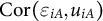) and the vertical axis is the average bias. We find that the estimators for all three modeling strategies that ignore sample selection are severely biased: the TTW and dummy variable strategies systematically underestimate the effect and the magnitude of this bias increases with $\rho $ , while the tiny value strategy substantially overestimates the effect across all values of $\rho $ . Both of the strategies that account for sample selection have minimal bias across the range of simulated circumstances.

Figure 2

Bias in $\hat {\beta }_{1A}$ —50% of districts partially contested.

Figure 2. Long description

The figure consists of four panels arranged in a two-by-two grid, labeled N equals 100, N equals 200, N equals 500, and N equals 800. Each panel has a horizontal x-axis representing rho ranging from 0.1 to 0.9 and a vertical y-axis representing Bias ranging from negative 1.0 to 1.5. A red dashed horizontal line marks the zero bias baseline.

Across all panels, five models are tracked:

- Tiny Value (open circle with dot, dash-dot line): Remains constant at the highest bias level of approximately 1.3.

- C M S (open square, solid line): Starts near 0.1 in the N equals 100 panel and converges toward the zero baseline as N increases, showing slight fluctuations around zero for higher N.

- Heckman (open triangle, long-dash line): Closely follows the zero baseline across all sample sizes, showing the least bias.

- T T W (open inverted triangle, dashed line): Shows a downward trend as rho increases, starting near negative 0.1 and dropping to approximately negative 0.6.

- Dummy Variable (asterisk, dotted line): Remains constant at the lowest bias level, starting near negative 0.7 and trending slightly downward to negative 0.9.

As the sample size N increases from 100 to 800, the C M S and Heckman models show tighter convergence toward the zero bias line, while the relative positions of Tiny Value, T T W, and Dummy Variable remain largely consistent.

Figure 3 presents the standard deviation of estimates from all five competing approaches. Across the board, the dummy variable and TTW strategies have the smallest standard deviation while the Heckman has the largest. The CMS and tiny value approaches perform much better than the Heckman and slightly worse than the other two. However, given the large amount of bias found for the TTW, dummy variable and tiny value strategies, the main comparison of interest in this figure is between the Heckman and CMS strategies.Footnote ²⁰ Because $\varepsilon _{iA}$ and $u_{iA}$ are not normally distributed, the standard deviation of Heckman estimates is larger, especially in relatively small samples. This shows that the CMS is more efficient than the Heckman. In Appendix D of the Supplementary Material, we demonstrate that the Heckman strategy also results in overconfidence, higher MSE and lower statistical power than the CMS.Footnote ²¹ Our approach consistently outperforms the Heckman model.

Figure 3

Standard deviation of $\hat {\beta }_{1A}$ s—50% of districts partially contested.

Figure 3. Long description

A four-panel grid of line graphs. Each graph shares a common Y-axis labeled Standard Deviation ranging from 0.0 to 1.0 and a common X-axis labeled with the Greek letter rho ranging from 0.1 to 0.9.

* Top-Left Panel (N = 100): The Heckman model (triangles, dashed line) shows the highest standard deviation, fluctuating between 0.8 and 0.9. Tiny Value (circles, dash-dot line) stays near 0.4. C M S (squares, solid line) is around 0.3. T T W (inverted triangles, short-dashed line) and Dummy Variable (asterisks, dotted line) are lowest, near 0.2.

* Top-Right Panel (N = 200): All values decrease. Heckman drops to approximately 0.6. Tiny Value is near 0.25. C M S, T T W, and Dummy Variable cluster between 0.1 and 0.2.

* Bottom-Left Panel (N = 500): Heckman further decreases to approximately 0.35. Tiny Value and C M S are near 0.2. T T W and Dummy Variable are near 0.1.

* Bottom-Right Panel (N = 800): Heckman is lowest here, near 0.25. Tiny Value and C M S are between 0.1 and 0.2. T T W and Dummy Variable are below 0.1.

Across all panels, as the sample size N increases, the standard deviation for all models decreases and the lines converge toward the bottom of the graph. A shared legend at the bottom identifies the models: C M S (square), Heckman (triangle), T T W (inverted triangle), Tiny Value (circle), and Dummy Variable (asterisk).

4.2 Results: Invalid exclusion restriction

To assess how the competing approaches perform when the exclusion restriction is violated, we repeat the experiment from the previous section, but set $\beta _{2A}=1$ such that $z_{2i}$ is no longer a valid instrument in Equation (14). Figure 4 presents bias in the estimates of $\beta _{1A}$ under this condition. The Heckman estimator is severely biased across all values of $\rho $ , performing much worse than models that ignore sample selection; the magnitude of this bias worsens as the sample size increases. The Heckman estimator is biased because, without the exclusion restriction, the inverse Mills ratio is nearly collinear with other regressors, which makes the Heckman estimator potentially un-identifiable in practice (Honoré and Luojia Reference Honoré and Luojia2024; Newey et al. Reference Newey, Powell and Walker1990; Sartori Reference Sartori2003; Wolfolds and Siegel Reference Wolfolds and Siegel2019).Footnote ²² In contrast, our CMS results in only slightly biased estimates when $\rho $ is large, but it still outperforms alternatives that ignore sample selection.

Figure 4

Bias in $\hat {\beta }_{1A}$ —invalid instrument and 50% of partial contestation.

Figure 4. Long description

Four panels arranged in a two-by-two grid represent sample sizes N equals 100, N equals 200, N equals 500, and N equals 800. Each panel has an X-axis labeled with the Greek letter rho ranging from 0.1 to 0.9 and a Y-axis labeled Bias ranging from negative 2.5 to 1.5. A horizontal red dashed line marks the zero bias baseline.

In all panels, five models are plotted with distinct line styles and markers.

* Tiny Value (dash-dot line with open circles) maintains a constant positive bias near 1.3.

* C M S (solid line with open squares) starts slightly above zero at rho equals 0.1 and trends downward to approximately negative 0.3 at rho equals 0.9.

* T T W (dashed line with downward triangles) stays below C M S, trending from negative 0.2 to negative 0.6.

* Dummy Variable (dotted line with asterisks) remains relatively flat near negative 0.8.

* Heckman (long-dashed line with upward triangles) shows the highest negative bias, positioned between negative 1.8 and negative 2.6.

As N increases from 100 to 800, the Heckman model's bias shifts further down the Y-axis, while the other models remain relatively stable in their vertical positions.

In Appendix D of the Supplementary Material, we show that without a valid instrument, the Heckman approach also performs poorly in terms of efficiency, overconfidence, coverage and power, whereas the CMS performs well across all these performance statistics.Footnote ²³ These results confirm that, under the distributional assumptions of error terms in compositional models derived from multinomial discrete choice processes, the Heckman correction is inappropriate if there is no valid instrument, a condition that is likely to happen in most empirical studies. Our CMS overcomes this limitation.

5 Application: Brexit and vote choice in England

We apply the CMS to analyze the English general elections in 2017 and 2019. Until the 2000s, elections in England yielded a suitable scenario to estimate compositional models as they revolved around two major parties (Labour and Conservatives) and a third force (Liberal Democrats, also known as Lib Dems), and all three parties fielded candidates in almost every district (Katz and King Reference Katz and King1999; Tomz et al. Reference Tomz, Tucker and Wittenberg2002). This situation has drastically changed as new parties, particularly the Greens and the UK Independence Party (UKIP), gained traction and became more competitive in some districts.Footnote ²⁴

The 2017 and 2019 elections followed the Brexit referendum in 2016. National politics was reshaped by the division between “leavers” (i.e., supporters of a quick solution for the UK’s departure from the European Union) and “remainers” (i.e., those who opposed Brexit). In both elections, the Conservatives were the party of the prime minister, held the majority of seats and were the main political force among the leavers.Footnote ²⁵ During these elections, Brexit changed the competitive dynamics between parties (Fieldhouse et al. Reference Fieldhouse2021). Rather than being viewed primarily as the incumbent party, the Conservatives were seen by most voters as the political force most able to implement Brexit. Hence, these two elections marked a transformation in long-term dynamics, such as economic voting and incumbency advantage, that had characterized English politics since the end of World War II (Kagalwala, Moreira, and Whitten Reference Kagalwala, Moreira and Whitten2024b). The leavers–remainers divide reduced the relevance of these previously stable voting patterns.

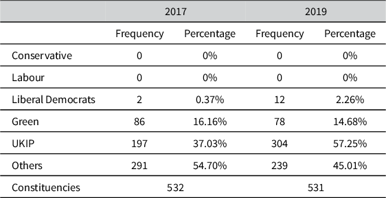
Partial contestation was high in 2017 and 2019 among small parties. Table 1 shows the frequency and the percentage of districts that parties did not contest.Footnote ²⁶ The Greens did not have a candidate in about 15% of districts in both elections. UKIP contested 63% of districts in 2017, but only 48.75% in 2019. A residual category “Others”—comprised of parties that did not receive at least 1% of overall votes and did not win legislative seats—fielded candidates in 54.7% and 45% of districts in 2017 and 2019, respectively.Footnote ²⁷

Table 1

Partial contestation by party and election

Table 1 Long description

The table compares the frequency and percentage of partial contestation across two election years, 2017 and 2019, for various political parties in the United Kingdom.

* Conservative: 0 frequency and 0% in both 2017 and 2019.

* Labour: 0 frequency and 0% in both 2017 and 2019.

* Liberal Democrats: 2 frequency (0.37%) in 2017, increasing to 12 frequency (2.26%) in 2019.

* Green: 86 frequency (16.16%) in 2017, decreasing to 78 frequency (14.68%) in 2019.

* U K I P: 197 frequency (37.03%) in 2017, increasing to 304 frequency (57.25%) in 2019.

* Others: 291 frequency (54.70%) in 2017, decreasing to 239 frequency (45.01%) in 2019.

The total number of constituencies recorded was 532 in 2017 and 531 in 2019.

Our CMS accounts for partial contestation as sample selection, allowing us to study how Brexit shaped trade-offs across all relevant parties. We use the Conservative Party as the baseline category of the log-ratios in Equation (2). Thus, the compositional outcome encompasses five log ratios, one for each $J-1$ category: the Labour Party, Liberal Democrats, Greens, UKIP and Others. For each of these parties, we estimate the following model specification:

(16) $$ \begin{align} \begin{aligned} {d}_{ijt} &= \alpha_{0j} + {\pmb{z}}_{ijt} {\pmb{\alpha}}_j + \varepsilon_{ijt}, \\ s_{ijt} &= \beta_{0j} + \phi_j s_{ijt-1} + {\pmb{x}}_{ijt} {\pmb{\beta}}_j + u_{ijt} , \end{aligned} \end{align} $$

where the first equation models j’s decision to contest district i in election t, and the second equation is the compositional outcome with $J-1$ log ratios. We estimate these equations jointly using the log-likelihood function in Equation (11).Footnote ²⁸ In the selection stage, $d_{ijt}$ is an indicator for whether j had a candidate in i, and ${\pmb {z}}_{ijt}$ is a vector of the following district-level covariates:

• • j’s distance in vote share from the second place in the previous election ( $t-1$ ),

• • the difference in vote shares between the top two parties at $t-1$ ,

• • the effective number of parties (ENP) at $t-1$ ,

• • the percentage of votes for leaving the European Union from the 2016 referendum,Footnote ²⁹

• • the percentage of residents claiming unemployment benefits in the district,

• • the log of the electorate size,

• • the share of the rural population,

• • dummy variables that indicate Conservative and Labour Party incumbency,

• • regional fixed effects,Footnote ³⁰ and

• • election fixed effects.

The first three variables in ${\pmb {z}}_{ijt}$ are tactical factors that a party j may consider when deciding whether to contest a district. We expect that smaller parties are less likely to employ scarce resources in localities where a single party dominates the contest. This is captured by the distance between the top two parties at $t-1$ . Similarly, j may avoid areas where its past electoral performances were poor and districts crowded with many contenders. We measure these factors with j’s distance from the runner-up and the ENP, both measured at $t-1$ . Because these first three variables are expected to affect parties’ contestation decisions but not the vote share of parties in districts that they contest, these variables are present in ${\pmb {z}}_{ijt}$ but not ${\pmb {x}}_{ijt}$ . Hence, they also play the role of meeting the exclusion restriction. The remaining variables in the list above are all expected to affect both the decision of parties about whether or not to contest a district and the percentages of support for parties that do contest them. Our equations for $s_{ijt}$ also include the temporally lagged dependent variable, $s_{ijt-1}$ , which both reflects our expectation of persistence over time and controls for unobservable common factors of a district that shape the trade-off between j and the baseline category (Keele and Kelly Reference Keele and Kelly2006).

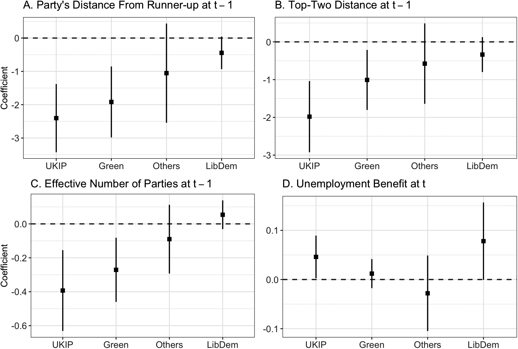
In Figure 5, we display estimated coefficients for four predictors in the selection equations. Each panel shows the coefficient of each predictor for the partially contesting parties.Footnote ³¹ As expected, the tactical variables affect the likelihood that small parties will contest a district. As the difference between the top two parties in the previous elections increases, the Greens and UKIP are less likely to field candidates (Panel A). Similarly, as the distance between their previous vote and that of the runner-up (Panel B) increases, they are less likely to contest districts, and as the ENP (Panel C) at $t-1$ increases, they are less likely to field candidates. Finally, Panel D shows that covariates in the outcome stage can also affect a party’s probability of fielding candidates. The unemployment variable is positively associated with the Liberals’ and UKIP’s decision to contest a district.

Figure 5

Coefficients in the selection stage.

Figure 5. Long description

The figure consists of four panels, each with a y-axis labeled Coefficient and an x-axis listing four categories: U K I P, Green, Others, and LibDem. A horizontal dashed line at zero serves as a baseline. Each data point is represented by a black square with vertical error bars indicating confidence intervals.

Panel A. Party's Distance From Runner-up at t minus 1: All coefficients are negative. U K I P is lowest at approximately minus 2.4, followed by Green at minus 1.9, Others at minus 1.1, and LibDem closest to zero at minus 0.4.

Panel B. Top-Two Distance at t minus 1: Similar to Panel A, all coefficients are negative. U K I P is at minus 2.0, Green at minus 1.0, Others at minus 0.6, and LibDem at minus 0.3.

Panel C. Effective Number of Parties at t minus 1: U K I P is at minus 0.4, Green at minus 0.27, and Others at minus 0.1. LibDem is the only positive coefficient in this panel, plotted slightly above zero at 0.05.

Panel D. Unemployment Benefit at t: The y-axis scale is smaller, ranging from minus 0.1 to 0.1. U K I P is positive at 0.05, Green is near zero at 0.01, Others is negative at minus 0.03, and LibDem is positive at 0.08. Most error bars in this panel cross the zero line.

Figure S1 in the Supplementary Material shows the estimated coefficients for Brexit votes and unemployment benefits across the $J-1$ outcome equations.Footnote ³² Consistent with Kagalwala et al. (Reference Kagalwala, Moreira and Whitten2024b), we find that support for Brexit increases the vote share of Conservatives to the detriment of parties that opposed leaving the European Union. Unemployment benefits, in turn, did not have the clear effect expected by economic voting theory.Footnote ³³ These coefficients, though, are in log-ratio form. We can use them for hypothesis tests about the trade-offs between parties, assessing the direction of the relationship and its statistical significance.Footnote ³⁴ To interpret the magnitude of these results, we transform them back into vote shares and calculate their associated confidence intervals using a non-parametric bootstrap in which we randomly sample the data 1,000 times with replacement. We calculate the difference in predicted vote share for each party after a one standard deviation increase $(+1\mathrm{SD})$ holding all other variables at their observed values.Footnote ³⁵

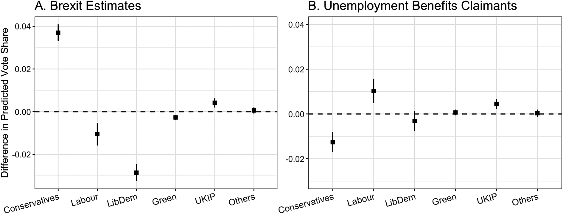
Figure 6 presents the effect of a $+1$ SD increase in Brexit votes (Panel A) and unemployment benefits (Panel B) on the predicted vote share for each party. This indicates that the Conservatives, as the major force supporting Brexit in 2017 and 2019, would win 3.7% of votes due to a $+1$ SD increase in estimated votes for Brexit in 2016. UKIP’s votes would also increase, but by a small degree, 0.4%. The Labour Party and Liberal Democrats would lose 1.1% and 2.8% of votes, respectively, from this increase in Brexit support. Panel B shows that the estimated changes in vote shares after a $+1$ SD increase in unemployment benefits are mostly smaller $-1$ % and $-1.2$ % for the Labour and Conservatives, respectively. UKIP also electorally benefited from a shock in unemployment (0.4%). These results support the expectation that the Brexit debate dominated U.K. politics in the 2017 and 2019 elections.Footnote ³⁶

Figure 6

Change in vote share in response to $+1$ SD shock.

Figure 6. Long description

The figure consists of two panels, A and B. Both panels share a y-axis titled Difference in Predicted Vote Share ranging from negative 0.02 to 0.04, with a dashed horizontal baseline at 0.00. The x-axis for both lists political parties: Conservatives, Labour, Lib Dem, Green, U K I P, and Others.

Panel A, titled Brexit Estimates:

* Conservatives: Positive point estimate near 0.038 with a small vertical error bar.

* Labour: Negative point estimate near negative 0.01 with an error bar crossing negative 0.015 to negative 0.005.

* Lib Dem: Negative point estimate near negative 0.028 with an error bar.

* Green: Slightly negative point estimate near 0.00.

* U K I P: Slightly positive point estimate near 0.005.

* Others: Point estimate at 0.00.

Panel B, titled Unemployment Benefits Claimants:

* Conservatives: Negative point estimate near negative 0.012.

* Labour: Positive point estimate near 0.01.

* Lib Dem: Slightly negative point estimate near negative 0.003.

* Green: Point estimate at 0.00.

* U K I P: Slightly positive point estimate near 0.005.

* Others: Point estimate at 0.00.

Table S2 in the Supplementary Material shows that the correlation between errors across stages is high $(>0.8)$ and statistically significant for all parties, demonstrating the necessity to account for sample selection: A party’s decision to contest a district and its vote share when it does contest that district are functions of correlated unobservables.