




No CrossRef data available.
ROBUST TESTS OF THE UNIT ROOT HYPOTHESIS SHOULD NOT BE “MODIFIED”
Published online by Cambridge University Press: 10 February 2004
Abstract
The rank-based unit root tests proposed by Hasan and Koenker (1997, Econometrica 65, 133–161) have power equal to size for normal innovations. Unit root tests based on M-estimators exhibit the same behavior. The problem occurs because the test statistics are transformed to obtain computationally convenient critical values. I describe a convenient way to compute critical values without transforming the test statistics. The resulting tests are almost as powerful as least squares–based tests for normal errors and much more powerful for thicker tailed distributions.I thank Thomas Rothenberg for many useful comments. This paper is based on my dissertation, which he supervised. I also thank Jack Porter, Jim Powell, Richard Stanton, and Jim Stock for good advice. Comments of Bruce Hansen, the editor, and two anonymous referees improved the exposition.
Information
- Type
- Research Article
- Information
- Copyright
- © 2004 Cambridge University Press
1. INTRODUCTION
Following Dickey and Fuller (1979), econometricians often employ least squares regression to test for a unit root in the autoregressive representation of a time series. Although least squares–based tests should perform well when the innovations are normal, there may be a loss of power relative to other methods when they are not normal. In recent years researchers have proposed a variety of “robust” tests that are designed to have good power for many different error distributions. For example, Cox and Llatas (1991), Lucas (1995a), Lucas (1995b), Hoek, Lucas, and van Dijk (1995), Herce (1996), and Rothenberg and Stock (1997) have proposed robust tests based on M-estimators; Hasan and Koenker (1997) have proposed a collection of rank tests.
Because the robust test statistics generally have null distributions that depend on unknown nuisance parameters, finding appropriate critical values is a nontrivial problem. Lucas (1995b) describes a simulation-based method for computing critical values. Herce (1996), Lucas (1995b), and Hasan and Koenker (1997) suggest transforming the test statistics so that the asymptotic null is nuisance-parameter free.
The present paper derives local-to-null asymptotic power functions for the robust tests and uses the asymptotic representations to evaluate the various procedures for computing critical values. The procedure in Lucas (1995b) leads to tests with incorrect size, even asymptotically. The transformations used in Herce (1996), Lucas (1995b), and Hasan and Koenker (1997) lead to tests with asymptotic power equal to size for normal errors. This result is not entirely new; Lucas (1995b) reports simulation evidence in favor of the result, and Herce (1996) derives a similar result for the test based on the least absolute deviations estimator.
I fit a polynomial approximation to the critical values of the untransformed test statistics. The resulting tests are almost as powerful as least squares for normal errors and much more powerful for thicker tailed distributions. For alternatives far from the null, the tests dominate the transformed statistics used by Herce (1996) and Hasan and Koenker (1997). A Monte Carlo study suggests that the untransformed versions of the Wilcoxon ranks and normal ranks tests of Hasan and Koenker (1997) are superior to the least squares tests for a variety of error distributions.
2. LOCAL-TO-UNITY ASYMPTOTICS FOR ROBUST TESTS
The observations {yt}t=1T come from the data generating process

where {εt}t=1T is an independent and identically distributed (i.i.d.) sequence with mean 0 and variance σε2. The term Γ(L) is the lag polynomial 1 − Γ1 L − ··· − Γp Lp, and we assume that the roots of Γ(z) = 0 all lie outside the unit circle. For convenience we assume that u0 = 0. We wish to test the unit root hypothesis γ = 0 versus the alternatives γ < 0.
The tests are based on the augmented Dickey and Fuller (1979) representation of the model

where ΔY = (yp+2 − yp+1,…,yT − yT−1)′, X = (yp+1,…,yT−1)′, and Z is the design matrix with row t − p − 1 equal to (1,t,Δyt−1,…,Δyt−p). The parameter α is γΓ(1), β is a (p + 2) × 1 parameter vector, and ε = (εp+2,…,εT)′. For the intercept only model (e.g., μ2 = 0) the design matrix Z has rows (1,Δyt−1,…,Δyt−p).
M-tests are based on M-estimators, which may be characterized as solutions to minimization problems. It will be convenient to adopt the notation that, for any function g(·) mapping

and any n-dimensional column vector x with components xi, g(x) is the n-dimensional column vector with components g(xi). The M-estimators

minimize the objective function

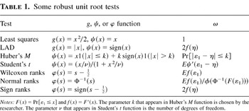
where 1 is a vector of ones and g is a function chosen by the researcher. When g(x) = x2, estimation is by least squares. Table 1 lists some alternative choices for g that “robustify” the estimators against thick-tailed error distributions. The unit root test rejects the null for small values of

.
Some robust unit root tests

Hasan and Koenker (1997) propose an alternative class of unit root tests based on ranks. The null is rejected for small values of [X′MX]−1/2X′Mb, where M is the projection matrix I − Z(Z′Z)−1Z′ and b is the vector of regression rank scores

, where

solves the linear programming problem

and φ is a function chosen by the researcher. This construction for b is a way to handle the nuisance parameters β and allows the researcher to consider general functions of the ranked residuals: when Z is a vector of ones and φ(τ) = τ, each element of b is the rank of the corresponding element of ΔY. Table 1 lists some common choices for φ.
In large samples the critical values and power functions of the various tests depend on several nuisance parameters. For the M-tests the nuisance parameters are determined by a scorelike function ψ(x), equal to g′(x) if g is differentiable at x and zero otherwise (we allow g to have finitely many points of nondifferentiability to handle quantile estimators such as least absolute deviations (LAD)). The nuisance parameters are

where

, f is the marginal density of ε1, and η solves Eψ(ε1 − η) = 0. When ψ is everywhere differentiable ω takes the more familiar form Eψ′(x − η). The rank tests depend on the same nuisance parameters, with ψ(x − η) replaced by φ(F(x)), where F(x) = Pr[ε1 ≤ x] . Table 1 lists the g, ψ, and φ functions for some common robust tests, along with the associated formulas for ω.
The tests come in two versions, an e-test and a t-test. The e and t M-tests reject the null for small values of the statistics

where the variables with the [caret ] are consistent estimates of the corresponding nuisance parameters. The e and t rank tests reject for small

Hasan and Koenker (1997) propose only the t version of the test, but for completeness we examine the e version also. Section 4 provides estimates of the nuisance parameters.
Hasan and Koenker (1997) stress that the nuisance parameter λ does not need to be estimated to normalize a rank test. This may be an advantage of the rank tests over the M-tests. In the Monte Carlos in Section 5, the rank tests have more accurate size than the M-tests. Thompson (2004b) argues that this occurs because of estimation error associated with

. Although in large samples the estimation error will have an asymptotically negligible effect on inference, in small samples it could affect test size. In some cases ω is especially poorly estimated—for example, for LAD ω = 2f (η), and the estimate of a density at a point converges at less than a root-T rate.
Because I am interested in inference when γ is close to one, I adopt the local-to-zero reparameterization γ = c/T so that the parameter space is a shrinking neighborhood of zero as the sample size grows. Following Chan and Wei (1987) and Phillips (1987), I take c fixed when making limiting arguments, obtaining asymptotic representations as a function of the local alternative c.
Hasan and Koenker (1997) derive local-to-zero asymptotic representations for the rank tests. In Theorem 1 I provide local-to-zero representations for the M-tests. The theorem applies to objective functions g that are not twice continuously differentiable, such as LAD, Huber's M function, and the quantile regression estimator of Koenker and Bassett (1978). We assume that g is convex, which rules out Student's t objective function. Although the convexity assumption simplifies the proof, alternative methods can be used to show that the theorem holds for Student's t function.
The limiting forms of the test statistics are expressed as functionals of Brownian motion. Define W(·) as standard Brownian motion and define Wc(·) as the Ornstein–Uhlenbeck process

. Define

where Dc(r) = Wc(r) −

in the intercept only model and

in the model with a linear time trend. Under the local-to-null asymptotics, the e-tests Me and Re both converge to the limiting distribution represented by the random variable

, and the t-tests Mt and Rt converge in distribution to the random variable

. The limiting forms are

where S is an independent standard normal variable. These results are summarized in the following theorem.
THEOREM 1. Under Assumptions 1 and 2 in the Appendix, Me and Re converge weakly to

, and Mt and Rt converge weakly to

.
There are a number of well-known asymptotic results concerning robust inference for a location model (see Rothenberg and Stock, 1997, Appendix). Asymptotic power depends on a single parameter that shifts the limiting distribution of the test statistic. Power is increasing in the parameter, which is maximized under correct specification. The movement of the parameter is asymmetric under incorrect specification, in the sense that with normal data power declines only slightly when using robust methods instead of least squares, but with thick-tailed distributions robust tests lead to significant increases in power.
For the unit root testing problem, large sample power depends on the pair of nuisance parameters ρ and λ. Because we reject for small values of the test statistics, in large samples the power of an e-test is given by

, where qe(ρ,a) satisfies

and a is the size of the test. Limiting power for the t-test is

, where

. Power obviously increases with λ, which shifts the distribution to the left when c is negative. The term ρ also affects power by changing the shape of the distribution. The results in Section 3.1 suggest that λ dominates the power function relative to ρ.
In general ρ and λ depend on the test and error density. An exception to this is the least squares–based Dickey–Fuller test, where ψ(x) = x and ρ = λ = 1 no matter what the error density. For other tests ρ will differ from 1 and the limiting null representations become a linear combination of a “Dickey–Fuller” term (Bc−1Ac for the e-test and Bc−1/2Ac for the t-test) and another random variable.
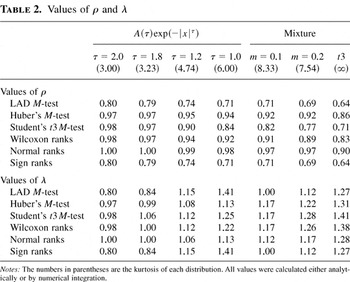
In Table 2 we have calculated ρ and λ by numerical integration for various tests and error densities.1
Numerical integration was carried out using the Matlab function quad, which implements a quadrature algorithm. All integrals were solved between −40 and 40, so, for example, ω was calculated as

for the Wilcoxon scores tests. Kurtosis is defined to be E [(ε − Eε)4]/Var(ε)2. We calculate the quantity by numerical integration.
Values of ρ and λ

To get a sense of how the parameters change as we move from normal errors to thicker tailed densities, we give results for error densities of the form f (ε) = A(τ)exp(−|ε|τ) for τ = 2.0, 1.8, 1.2, and 1.0 and for the thick-tailed Student's t distribution with three degrees of freedom (denoted t3).2
The normalizing constants A(τ) are chosen to make the densities integrate to one.
The values of ρ fall as the errors become thicker tailed. For normal errors the parameter is close to 1, except for the LAD and sign rank tests. Under normality the null distributions of the other tests are similar to the null for the least squares–based tests. When the errors have thick tails the null distributions are different from the least squares distributions and from each other.
The term λ increases as the errors become thicker tailed, suggesting that thicker tailed errors lead to increased power. Under normal errors the parameters for the LAD and sign-median rank tests are far below 1, so we expect these tests to have poor power relative to the least squares–based tests when errors are normal. For the rest of the tests λ is close to 1 with normal errors, implying that these tests have power almost as good as least squares when errors are normal and better than least squares when errors are thick tailed. Table 4 confirms this analysis; there the robust tests essentially dominate least squares, even for distributions close to Gaussian.
For the test and errors densities considered in Table 2, λ is maximized by choosing −ψ(x − η) or −φ(F(x)) equal to ∂ log f (x)/dx. For normal errors, λ is largest with the least squares and normal ranks tests. The same result holds for the LAD and sign ranks tests used with double exponential errors and for the t3 test with t3 errors. This property holds for any test and error distribution, which is not surprising because it corresponds to testing under correct specifying of the error distribution. To see that it holds for the rank tests, let f (x) equal

, where A makes the density integrate to one. An argument based on integration by parts can be used to show that ω = σψ2. For any

with associated

, we have

Therefore

. The result can be extended to the M-tests by replacing φ(F(x)) with ψ(x − η).
It can be shown, using integration by parts, that ρ = λ−1 when −ψ(x − η) or −φ(F(x)) equals ∂ log f (x)/dx. This may be confirmed in the tables for the least squares and normal ranks tests applied to Gaussian errors. It may also be confirmed for the LAD and sign ranks tests used with double exponential errors and for the t3 test with t3 errors. Thus, under correct specification of the errors only one nuisance parameter appears in the asymptotic representation of the test statistics.
3. OBTAINING CRITICAL VALUES
It is well known that the asymptotic null distributions of the usual Dickey–Fuller tests do not depend on any nuisance parameters. Critical values can be calculated once and tabulated. For robust, non-least squares–based tests, the critical values cannot be tabulated so simply. The asymptotically correct critical values qe(ρ,a) and qt(ρ,a) are the ath quantiles of

. For a given robust test ρ must be estimated, so the shape of the asymptotic null distribution is not estimable until we see the data.
There are many ways to accurately approximate the quantiles of

. Shin and So (1999) simulate draws of

for each ρ and use the empirical quantiles as critical values. Seo (1999) and Lucas (1998) also describe simulation-based procedures. Rothenberg and Stock (1997) and Thompson (2004b) use Cornish–Fisher expansions. Hansen (1997) and Juhl and Xiao (2002) simulate to calculate quantiles for similar test statistics.
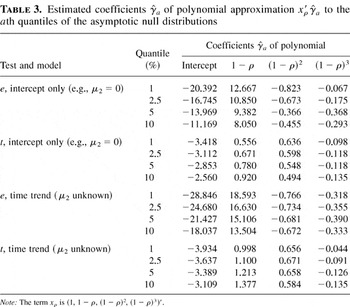
A computationally convenient approach is to approximate qe(ρ,a) and qt(ρ,a) by a third-order polynomial in 1 − ρ. For the

statistic the formula is

where xρ = (1, 1 − ρ, (1 − ρ)2, (1 − ρ)3)′ and γa is a four-dimensional coefficient vector. The formula is defined similarly for the

-statistic. To compute γa I simulated N = 5 million draws of

for ρ = ρ0,…,ρ100, where ρj = j/100.
3Throughout the paper simulations from the distributions of Ac and Bc were computed as the realizations of normalized sums of 500 successive draws from a discrete time Gaussian AR(1) process with autoregressive parameter 1 − c/T.

as the (aN)th draws of the simulated statistics. For the

test I compute γa by regressing

on xρj. The minimization problem is

The same procedure is used for

. Table 3 provides the estimated coefficients for a equal to 0.01, 0.025, 0.05, and 0.10.
Estimated coefficients of polynomial approximation to the ath quantiles of the asymptotic null distributions

Local alternative where asymptotic power is approximately 50%

In practice I calculate critical values using a consistent estimate

for ρ. So the e-tests reject the null at level a when Me or Re are less than

. Similarly the t-tests reject when Mt or Rt are less than

. The estimation of

and the other nuisance parameters is discussed in Section 4.
Figure 1 plots the simulated quantiles along with the polynomial approximations. The quantiles are nearly linear in ρ, and it is difficult to see a difference between the quantiles and the approximating polynomial. I assess the quality of the approximation in terms of the worst large sample size distortion:


Simulated 1%, 2.5%, 5%, and 10% quantiles (solid lines) plotted along with the polynomial approximations from Table 3 (dotted lines). The approximations are so close that it is difficult to distinguish the solid from the dotted lines. The horizontal axes give values of ρ.
The expression

is an estimate of

. I calculate

by simulating 5 million draws of

, independent of the draws used to estimate γα, and calculate

as the percentage of draws below z. The worst size distortion was calculated for the models with and without a trend and for both the

- and

-statistics. The maximum over the four cases was 0.0004942. Thus the polynomial approximations are highly accurate both in terms of approximating the quantiles and minimizing asymptotic size distortions.
3.1. Modifying the Tests to Eliminate the Nuisance Parameter
Herce (1996) and Hasan and Koenker (1997) suggest modifying the test statistics to obtain null distributions that are free of ρ. Recall that

are expressed as linear combinations of the “Dickey–Fuller” terms A0 /B0 and

and another random variable. Because the least squares test statistics converge to the Dickey–Fuller terms, we can write down a linear combination of the robust test statistics and of the least squares statistics so that the limiting null distribution does not depend on ρ. Let els and tls denote the me- and mt-statistics when estimation is by least squares. The modified tests are based on the relationships

where

is a consistent estimator for ρ. A test that rejects the null when the modified statistics are below the 100a% quantile of S/B01/2 or S will have asymptotic size equal to a. The rank tests may be similarly modified.
Unfortunately, this modification seriously affects the power of the tests. Let Φ and φ denote the distribution function and density function of a standard normal variable. When the errors are i.i.d. normal, the rank test formula for λ is

The same result holds for the M-tests. Thus, under normal errors λ = ρ no matter what the test, so the modified t-test has local power everywhere equal to its size. This may be confirmed in Table 2, where under normality λ equals ρ for every test considered. In Table 4 we also show that the modified e-test also has very little power with normal errors. Lucas (1995b) reports simulation results for M-tests that are consistent with these results. Herce (1996) obtains a stronger result for the LAD estimator—under normal errors the modified LAD t-test has power equal to its size. Although our results apply only to the local power function, in Section 5 we provide Monte Carlo evidence that the actual power function exhibits similar behavior for empirically relevant sample sizes. Robust methods are meant to perform well for plausible misspecifications of the model. By this measure the traditional Dickey–Fuller methods are robust relative to the modified statistics.
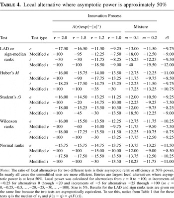
Table 4 provides some evidence to compare the modified tests with the unmodified tests that use the polynomial approximation to the critical value. The table lists the local alternative where asymptotic power is approximately ½ in the model that includes a linear time trend (e.g., no restrictions on μ2). King (1988) and Elliott, Rothenberg, and Stock (1996) make the case for preferring tests that achieve 50% power at alternatives closer to zero. By definition, tests that achieve 50% power at lower values of c have better asymptotic relative efficiency at 50% power (see Stock, 1994, p. 2775).
The modified tests have virtually no power for distributions close to the Gaussian, but sometimes they beat the unmodified tests for the thick-tailed double exponential and t3 errors. Asymptotic power was calculated for local alternatives as small as −100, so a value of −100 in the table means that the test did not achieve 50% power for any alternative greater than −100. Although the modified e-test has power greater than size for Gaussian errors, the modified e-tests considered here do not achieve 50% power for any alternative greater than −100. Both the modified and unmodified e-tests beat the corresponding t-tests for error distributions close to normality, and the t-tests are more powerful for thicker tailed error distributions.
The unmodified robust tests essentially dominate least squares. The least squares–based e- and t-tests of Dickey and Fuller (1979) achieve 50% power at c = −15.75 and −17.5; the unmodified robust tests do slightly worse for normal errors and much better for nonnormal errors. For each robust test the presence of thick-tailed errors leads to greater power relative to normal innovations. There is a larger decline in power under normality for the LAD and sign ranks tests, but even in these two cases the decrease is small relative to the gain in power for thicker tailed distributions.
The normal ranks test is at least as efficient as the least squares test for every error distribution in the table. In the classical location model we can make the stronger statement that the normal ranks test is asymptotically at least as powerful as the least squares t-test no matter what the error distribution. This result is shown by Chernoff and Savage (1958) (also see the discussion in Hettmansperger, 1984, Sec. 2.9). The result may hold for the unit root problem, but I was not able to prove it. At normal errors both the Dickey–Fuller and the normal ranks tests have λ = ρ = 1, so their power functions are identical. I am able to show that for the normal ranks test, λ ≥ 1 and ρ ≥ 1/λ for any error distribution. Power obviously increases in λ, but simulations show that power is not monotonic in ρ. However, I conducted simulations4
I carried out the following simulation. Set ρi = i/50, λj = 50/j, and ck = −k. For each (ρ, λ, c) = (ρi, λj, ck) triple over i = 1,…,50, j = 1,…,50, k = 1,…,50, I simulated 100,000 Monte Carlo draws of

. For each c I computed power for a 5% level test using the polynomial approximations to the critical values given in Table 3.
Chernoff and Savage (1958) establish that λ ≥ 1 for the normal ranks test; see for example their Theorem 3 or Theorem 2.9.2 of Hettmansperger (1984). To see that ρ ≥ 1/λ, note that σψ2 = 1 and assume without loss of generality that σε2 = 1. Thus

where f is the density of the errors and φ is a standard normal density. The second equality follows from the change of variables x = Φ−1(F(y)), and the third equality follows from the fact that ∂φ(x)/∂x = −xφ(x). Integration by parts and a change of variables leads to the expressions

Let W = f (ε1)/φ(Φ−1(F(ε1))). By Jensen's inequality,

3.2. Lucas's (1995b) Method for Obtaining Critical Values
Lucas (1995b) obtains critical values by computing the distribution of the test statistics from realizations of simulated data. Lucas simulates the data by generating a time series from the data generating process with i.i.d. standard normal innovations vt and with dt and γ set to zero. Because the parameter ρ depends on both the choice of estimation method and the error density, this approach will give asymptotically incorrect critical values for the robust tests unless the errors are in fact normal. For the tests based on the t3 estimator, ρ = 0.98 for normal errors and the 5% quantiles of

are −21.8 and −3.42 when the model has a time trend. For t3 errors ρ = 0.71 and the quantiles are −17.5 and −3.01. A simulation shows that when the errors are distributed t3, using the quantiles based on normal errors instead of the correct values results in e- and t-tests with asymptotic sizes of 1.59% and 1.68%, respectively.
5There are 50,000 Monte Carlo replications.
4. CALCULATING THE TESTS
To calculate the test statistics we need consistent estimates for the various nuisance parameters. Likewise, the polynomial approximation to the critical values,

, is evaluated at a consistent estimate

for ρ.
Following Hasan and Koenker (1997), the nuisance parameters are estimated under the null. For a given M-test with associated functions g and ψ, let

denote the vector of residuals

, where

minimizes 1′g(ΔY − Zβ). Theorem 1 implies that under the null,

will converge to the recentered errors ε − η. So we estimate the two variances σε2 = Var(ε1) and σψ2 = Var(ψ(ε1 − η)) with

where

are the sample averages of

. Similarly, the correlation ρ = Corr[ε1,ψ(ε1 − η)] is estimated by

For Huber's M-test and the t3-test ω is estimated by

, where ∇ψ(x) equals ψ′(x) if ψ is differentiable at x and zero otherwise. Following Herce (1996), for the LAD test I estimate ω = 2f (η) using the kernel estimator

, where

. The bandwidth h was chosen based on a recommendation in Silverman (1986, Ch. 2). The term

will converge in probability to f (η) because

is converging to ε − η. Following Lucas (1995b), the scale parameter k appearing in Huber's M function is

, where

are the residuals from a preliminary LAD regression.
For the rank tests the nuisance parameters are calculated using the same formulas. I follow Hasan and Koenker (1997) and set the residuals

equal to

, where

minimizes the LAD objective function 1′|ΔY − Zβ|. For the rank tests ψ(x) is replaced by

, where

is an estimate of F. Following Hasan and Koenker (1997), I take

to be the empirical distribution function of

, equal to ({#residuals ≤ x} − 0.5)/(T − p). The term σψ2 is known in closed form for the rank tests and does not need to be estimated; σψ2 is

for the Wilcoxon ranks test and 1 for the normal and sign ranks tests.
Computing the rank tests requires calculating the vector

, where

solves the linear programming problem in (2). Hasan and Koenker (1997) use an algorithm that calculates

for all s. I instead solve the linear programming problem in expression (2) at the points {τi}i=150 (with τi = (i − 1)/49) and use numerical integration. For the Wilcoxon ranks test,

. For the normal ranks test, b is

and for the sign ranks tests it is

. I use the discretized version of the

process because canned algorithms for solving linear programming problems are widely available—for example, I used the Matlab function linprog.
5. MONTE CARLO EVIDENCE
We carried out a Monte Carlo study to evaluate the small sample performance of the various tests. The calculation of the various tests was described in Section 4.
Table 5 lists empirical rejection rates under the null (γ = 0) and for a distant alternative (γ = −0.5). The errors εt are i.i.d. draws from either the N(0,1) or Student's t3 distribution. We make the unrealistic assumption that the researcher knows that the errors are i.i.d. and sets the lag length p equal to zero. Results are given for both the intercept only model and for the model with a time trend. Small sample size looks good for all the tests except the modified e. The LAD test exhibits some size distortions. Thompson (2004b) argues that this results from a poor estimate of ω, because

does not converge at a root-T rate.
Empirical rejection rates, i.i.d. errors

Previously we have shown that the modified tests have poor power against the local alternative c. The Monte Carlo results suggest that power is also poor against the distant alternative γ = −0.5. Test power is very close to one for most of the unmodified tests, whereas the modified tests suffer from large power losses. As the asymptotics predict, the modified t-tests have power equal to size for normal errors. The asymptotics also predict that the modified tests will beat the unmodified ones for the thick-tailed Student's t3 distribution, and this does not seem to be the case. One explanation for this is that the local-to-null asymptotic approximations become less accurate for distant alternatives such as γ = −0.5. Thus the Monte Carlo results make a stronger case against the modified tests than the asymptotics.
The calculations in Table 5 assume that the errors are independent. To investigate the impact of serially correlated errors, Table 6 provides evidence about the small sample behavior of the unmodified tests when the errors exhibit serial dependence of unknown form. The data generating processes are

Empirical rejection rates with serially correlated errors

The fundamental innovations ζt have initial condition ζ0 = 0 and were generated from either the N(0,1) or the t3 distribution. The table gives results for the intercept only model and also for the model that includes a time trend.
Bringing the tests to serially correlated data requires an algorithm for selecting the lag length p. The term p is chosen by the Bayesian information criterion of Schwarz (1978) constrained so 2 ≤ p ≤ 6. Because the tests are designed for thick-tailed data, we calculate Schwarz's criterion from a double-exponential likelihood with constant variance.
Size is generally accurate for AR errors, less accurate for MA errors, and worse for GARCH errors. The t-tests exhibit more accurate size than the e-tests. For the rank t-tests, rejection rates under the null range from 0.04 to 0.11. The rank tests in general exhibit better size properties than the M-tests. Thompson (2004b) argues that this occurs because of estimation error associated with

. Computing the rank tests does not require an estimate of

. Although in large samples the estimation error will have an asymptotically negligible effect on inference, in small samples it could affect test size.
As the asymptotic analysis predicted, the robust tests essentially dominate least squares at the alternative γ = −0.1. Except for the LAD and sign ranks tests, the robust tests are about as good as least squares at normal errors and are much more powerful at t3 errors. The asymptotics also suggested that the e-tests would be more powerful than the t-tests for normal errors but less powerful for t3 errors, but in the Monte Carlo the e-tests are at least as powerful as the t-tests for both distributions. Taking the size and power results together, the unmodified Wilcoxon ranks and normal ranks t-tests are nice alternatives to least squares: both rank tests have accurate size, and both do at least as well as least squares over a range of error distributions.
6. CONCLUSION
A goal of the robustness literature is to produce a test that is almost as powerful as least squares–based tests for normal errors and much more powerful for thicker tailed distributions. Although the modified tests have poor power, unmodified tests can achieve this goal. Shin and So (1999) document large power gains from using tests that adapt to the shape of the error distribution. Thompson (2004a) provides examples where the robust tests are more powerful than the point-optimal DF-GLS test of Elliott et al. (1996). Thompson (2004b) constructs confidence intervals for the parameter c by inverting the rank t-test Rt. Under normality the robust intervals are almost as short as the least squares–based intervals of Stock (1991) and Elliott and Stock (2001), and under nonnormal distributions the robust intervals tend to be much shorter.
APPENDIX
Here we prove Theorem 1. We will derive the results for M-estimators for the model with a linear time trend. All of the results may be extended to the model with an intercept only (e.g., μ1 = 0). The required results for the rank tests are contained in the Appendix to Hasan and Koenker (1997). Throughout the Appendix ∥·∥ denotes the norm: ∥bij∥ = ([sum ]i,j bij2)1/2.
To incorporate estimators based on the LAD and Huber's M function, we allow g to have finitely many points of nondifferentiability if continuity and several growth conditions hold. We assume that g is convex because it simplifies the proofs. The proofs rely on an asymptotic approximation to the objective function, and assuming convexity allows us to conclude that our approximation, which is proved keeping the parameters fixed, holds uniformly over the parameters in a neighborhood of their true values. Convexity also greatly simplifies the demonstration of the rate of convergence of the estimators. Our extensive use of convexity is due to results in Pollard (1991) and Hjort and Pollard (1993). Some objective functions, such as the Student's t, are not convex. Because this objective function is three times differentiable, the usual Taylor series–based arguments can be used to show that Theorem 1 holds for this objective function.
Assumption 1 (Objective Function). g(x) is convex and strictly increasing in |x|; g(x) is everywhere twice differentiable except for x in P, where P contains the D points p1,…,pD. g satisfies the Lipshitz condition |g(x) − g(y)| ≤ H|x − y|. |ψ(x)| ≤ H, and there exist two finite points xL and xH so that ψ(x) is constant for x > xH and for x < xL. The term |g′′(x)| < H for x not in P.
This assumption rules out the least squares estimator, because the squared error function g(x) = x2 does not satisfy the Lipschitz condition.
Because g may not be everywhere differentiable, we cannot use the usual Taylor series expansions to approximate the objective function. Instead of pointwise differentiability, the proofs make use of stochastic differentiability as in Pollard (1985). This requires that I impose smoothness conditions on the error density to make up for the lack of smoothness in the objective function.
Assumption 2 (Smoothness of the Error Density). The errors {εt}t=1T are i.i.d. mean zero with E|ε1|2+δ < H for some δ > 0. The term ε1 has a density function f (z) that is bounded and uniformly continuous.
It will prove convenient to reparameterize the objective function. Consider the estimator

that minimizes [sum ]t=p+2 qt(θ), where

Here wt′ = T−1/2(ut−1 /T1/2,1,t/T,Δut−1,…,Δut−p)′ and

is a 3 + p-dimensional parameter vector given by

for i = 1,…,p. Because there is a one-to-one mapping between

, we will describe the asymptotic properties of

.
Define the remainder term

The following two lemmas establish that rt(θ) is asymptotically negligible, implying that the objective function is approximately quadratic.
LEMMA 1. Define bt = 1(T1/2∥wt∥ > M). For any ε > 0, we can take M large enough so that limT→∞ Pr[|[sum ] rt(θ)bt| > ε] < ε.
Proof. Write the remainder as [sum ] rt(θ)bt = [sum ] Et−1 rt(θ)bt + R0,T, where R0,T = [sum ](rt(θ) − Et−1 rt(θ))bt. To handle the Et−1 rt(θ)bt term, define the function h(u) = Et−1 [g(εt − η + u) − g(εt − η)] , or equivalently

We have imposed enough smoothness on g, ψ, and f so that h(u) is twice continuously differentiable. By a Taylor series expansion,

where |ut*| ≤ |wt′θ|. Notice that h(0) = 0, h′(u) = Et−1 [ψ(εt − η + u)] , and h′(0) = 0. The term h′′(u) can be shown to be −∫ψ(x − η + u) df (x) by an argument based on integration by parts. The boundedness of f along with the conditions on ψ in Assumption 1 imply that there exists a bound B so that supu|h′′(u)| < B. Therefore

By Hölder's inequality,

where ε(M) = supt Pr[T1/2∥wt∥ > M] . For all t, T1/2wt converges to an Op(1) random variable, so E(T1/2θ′wt)2+δ is bounded and ε(M) → 0 as M increases. Thus we can pick M large enough to make the term small with high probability.
Next we handle the R0,T term:

The Lipshitz condition on g implies that |rt(θ)| ≤ (2H + |ψ(εt − η)|)|wt′θ|. Therefore

We showed in equation (A.2) that we can pick M large enough to make E [sum ](wt′θ)2bt asymptotically negligible. █
LEMMA 2. For any fixed M,

.
Proof. It will prove convenient to examine the remainder over regions where it is differentiable and regions where it is not differentiable. Let

denote wt1(T1/2∥wt∥ < M) and let At denote the event that

for all i. So

is differentiable in θ. Write the remainder as [sum ] rt1(T1/2∥wt∥ < M) = R2,T + R3,T + R4,T, where R2,T = [sum ][1(At)zt(θ) − Et−11(At)zt(θ)], R3,T = [sum ][1(Atc)zt(θ) G− Et−11(Atc)zt(θ)] ,

and

.
A Taylor series expansion yields

where

. Because R2,T is a sum of martingale difference sequences,

Therefore limT→∞ ER2,T2 = 0, so R2,T converges in probability to zero.
The condition 1(Atc) = 1 puts a bound on the values εt can take. Therefore the moment E1(Atc)zt2 exists. For large enough T,

Because the density of ε1 is bounded, limT→0 ER3,T2 = 0 and |R3,T| converges to zero in probability.
To handle R4,T, define h(u) as in (A.1). By a Taylor series expansion of h around 0,

The continuity of h′′(u) leads to the result limT→∞{supt|h′′(0) − h′′(ut*)|} = 0, with supt|ut*| < T−1/2M∥θ∥. The term ω can be shown to be equal to h′′(0) using an argument based on integration by parts. Thus R4,T converges to zero in probability. █
Proof of Theorem 1. Hasan and Koenker (1997) prove the result for the rank test statistics Re and Rt. To deal with the M-statistics Me and Mt, combine Lemmas 1 and 2 to obtain the pointwise convergence result

. By the convexity of g and Lemma 1 of Hjort and Pollard (1993), if

for fixed θ then the convergence is uniform over θ in compact sets. Uniform convergence of the remainder, combined with the argument in Section 3 of Pollard (1991), leads to the asymptotic approximation

Lemma 3.1 of Phillips (1988) implies the weak convergence result

where

is standard Brownian motion, independent of W. The desired results follow from the usual applications of the continuous mapping theorem. █
References
REFERENCES
Chan, N.H. &
C.Z. Wei
(1987)
Asymptotic inference for nearly nonstationary Ar(1) processes.
Annals of Statistics
15,
1050–1063.Google Scholar
Chernoff, H. &
R. Savage
(1958)
Asymptotic normality and efficiency of certain nonparametric test
statistics.
Annals of Mathematical Statistics
29,
972–994.Google Scholar
Cox, D.D. &
I. Llatas
(1991)
Maximum likelihood type estimation for nearly nonstationary
autoregressive time series.
Annals of Statistics
19,
1109–1128.Google Scholar
Dickey, D. &
W. Fuller
(1979)
Distribution of estimators for autoregressive time series with a
unit root.
Journal of the American Statistical Association
74,
427–431.Google Scholar
Elliott, G.,
T. Rothenberg, &
J.H. Stock
(1996)
Efficient tests for an autoregressive unit root.
Econometrica
64,
813–836.Google Scholar
Elliott, G. &
J.H. Stock
(2001)
Confidence intervals for autoregressive coefficients near one.
Journal of Econometrics
103,
155–181.Google Scholar
Hansen, B.E.
(1997)
Approximate asymptotic p values for structural-change
tests.
Journal of Business and Economic Statistics
15,
60–67.Google Scholar
Hasan, M.N. &
R.W. Koenker
(1997)
Robust rank tests of the unit root hypothesis.
Econometrica
65,
133–161.Google Scholar
Herce, M.A.
(1996)
Asymptotic theory of LAD estimation in a unit root process with
finite variance errors.
Econometric Theory
12,
129–153.Google Scholar
Hettmansperger, T.P.
(1984)
Statistical Inference Based on Ranks.
Wiley.
Hjort, H.L. &
D. Pollard
(1993)
Asymptotics for Minimizers of Convex Processes.
Preprint,
Department of Statistics, Yale University.
Hoek, H.,
A. Lucas, &
H.K. van Dijk
(1995)
Classical and Bayesian aspects of robust unit root inference.
Journal of Econometrics
69,
27–59.Google Scholar
Juhl, T. &
Z. Xiao
(2002)
Partially Linear Models with Unit Roots.
Discussion paper 1359,
Cowles Foundation.
King, M.L.
(1988)
Towards a theory of point optimal testing.
Econometric Reviews
6,
169–218.Google Scholar
Lucas, A.
(1995a)
An outlier robust unit root test with an application to the
extended Nelson-Plosser data.
Journal of Econometrics
66,
153–173.Google Scholar
Lucas, A.
(1995b)
Unit root tests based on m estimators.
Econometric Theory
11,
331–346.Google Scholar
Lucas, A.
(1998)
Inference on cointegrating ranks with LR and LM tests based on
pseudo-likelihoods.
Econometric Reviews
17,
185–214.Google Scholar
Phillips, P.C.B.
(1987)
Toward a unified asymptotic theory for autoregression.
Biometrika
74,
535–547.Google Scholar
Phillips, P.C.B.
(1988)
Regression theory for near-integrated time series.
Econometrica
56,
1021–1043.Google Scholar
Pollard, D.
(1985)
New ways to prove central limit theorems.
Econometric Theory
1,
295–314.Google Scholar
Pollard, D.
(1991)
Asymptotics for least absolute deviation regression estimators.
Econometric Theory
7,
186–199.Google Scholar
Rothenberg, T.J. &
J.H. Stock
(1997)
Inference in a nearly integrated autoregressive model with
nonnormal innovations.
Journal of Econometrics
80,
269–286.Google Scholar
Schwarz, G.
(1978)
Estimating the dimension of a model.
Annals of Statistics
6,
461–464.Google Scholar
Seo, B.
(1999)
Distribution theory for unit root tests with conditional
heteroskedasticity.
Journal of Econometrics
91,
113–144.Google Scholar
Shin, D.W. &
B.S. So
(1999)
Unit root tests based on adaptive maximum likelihood estimation.
Econometric Theory
15,
1–23.Google Scholar
Silverman, B.W.
(1986)
Density Estimation for Statistics and Data Analysis.
Chapman and Hall.
Stock, J.H.
(1991)
Confidence intervals for the largest autoregressive root in U.S.
macroeconomic time series.
Journal of Monetary Economics
28,
435–459.Google Scholar
Stock, J.H.
(1994)
Unit roots, structural breaks, and trends. In
R.F. Engle &
D.L. McFadden (eds.),
Handbook of Econometrics,
vol. 4, pp.
2739–2841.
Elsevier.
Thompson, S.B.
(2004a)
Optimal versus robust inference in nearly integrated non-Gaussian
models.
Econometric Theory
20,
23–55.Google Scholar
Thompson, S.B.
(2004b)
Robust confidence intervals for autoregressive coefficients near
one. In
Fetschrift in Honor of Thomas Rothenberg.
Cambridge University Press,
forthcoming.
Some robust unit root tests
Values of ρ and λ
Estimated coefficients of polynomial approximation to the ath quantiles of the asymptotic null distributions
Local alternative where asymptotic power is approximately 50%
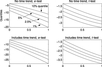
Simulated 1%, 2.5%, 5%, and 10% quantiles (solid lines) plotted along with the polynomial approximations from Table 3 (dotted lines). The approximations are so close that it is difficult to distinguish the solid from the dotted lines. The horizontal axes give values of ρ.
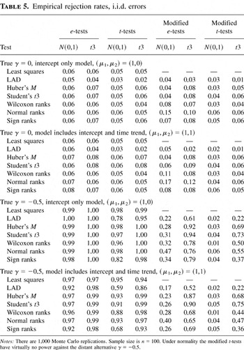
Empirical rejection rates, i.i.d. errors
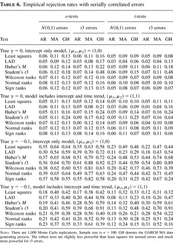
Empirical rejection rates with serially correlated errors
 You have
Access
- 12
- Cited by