





1. Introduction
Recently, several variants of kernel-based or weighted random connection models (RCMs) have received substantial research interest [Reference Gracar, Grauer, Lüchtrath and Mörters4, Reference Gracar, Heydenreich, Mönch and Mörters5, Reference Gracar, Lüchtrath and Mörters6, Reference Komjáthy and Lodewijks12]. This is because they can reproduce the heavy-tailed degree distributions observed in many real-world complex networks, while simultaneously retaining a positive clustering coefficient. This latter property sets them apart from standard discrete models for complex networks such as the Chung–Lu model or the Norros–Reittu model [Reference Aiello, Chung and Lu1, Reference Norros and Reittu20]. Other popular alternatives for obtaining a positive clustering coefficient include the spatial preferential attachment models [Reference Jacob and Mörters10, Reference Jacob and Mörters11]. While these models offer a natural interpretation of a growing network, their time-dependent construction makes them far less tractable than the weighted RCMs. Another highly studied class of spatial scale-free networks is the hyperbolic random geometric graph from [Reference Gugelmann, Panagiotou and Peter7], where the non-Euclidean geometry can pose technical difficulties. Such hyperbolic networks have Euclidean RCM counterparts, in the sense that these networks have the same local limits as some RCMs [Reference van der Hofstad29, Theorem 9.33], but it is not clear if local limits are sufficient to capture many interesting network properties such as the asymptotic normality of subgraph counts.
In this paper, we consider a popular example for such weighted RCMs, namely the age-dependent random connection model (ADRCM) [Reference Gracar, Grauer, Lüchtrath and Mörters4, Reference Gracar, Heydenreich, Mönch and Mörters5, Reference Gracar, Lüchtrath and Mörters6, Reference Komjáthy and Lodewijks12]. Here, nodes are placed in a metric space and endowed with independent and identically distributed (i.i.d.) weights, and the connection probability between two nodes is a function of both the distance and their respective weights, in such a way that the typical degree has a power law. The main achievements of this paper are normal approximation results for clique and subtree counts in the ADRCM. Our motivation is to investigate the limiting behavior of such networks in large domains, and such normal approximation results would statistically validate the use of the ADRCM as a model for real data. For example, with the help of the asymptotic normality obtained, we could derive asymptotic confidence intervals for such networks as the basis for various hypothesis tests. Even though the computations and regimes may not be identical to those for other RCMs, many of the methods used here have the potential to be deployed in other models, where the local number of subgraphs is square integrable.
Central limit theorems (CLTs) in spatial random systems have become a vibrant research stream in the last 20 years, from the martingale-based techniques in [Reference Baryshnikov and Yukich2], [Reference Penrose and Yukich23], and [Reference Yukich31] to the Malliavin-Stein method that allowed second-order Poincaré inequalities and likely optimal rates of convergence to be obtained; see [Reference Lachièze-Rey and Peccati14], [Reference Lachièze-Rey, Schulte and Yukich15], [Reference Last, Peccati and Schulte17], [Reference Reitzner and Schulte24], and [Reference Schulte and Yukich25] for related studies in this direction. However, these results traditionally require uniformly bounded fourth moments, which is not compatible with the heavy-tailed behavior of the ADRCM. We exploit here a recent update of the Malliavin–Stein method from [Reference Trauthwein27], [Reference Trauthwein28] that allows us to deal with functionals where only moments of order
 $(2+\varepsilon)$
are needed, and [Reference Oliveira21, Theorems 4.1 and 4.8] for associated random variables.
Last et al. [Reference Last, Nestmann and Schulte16] established a quantitative CLT for component counts. However, they assumed unweighted edges and results in a light-tailed (Poisson) degree distribution. In contrast, the major difficulties in our work stem exactly from the heavy-tailed nature of the degree distribution. While both this paper and [Reference Last, Nestmann and Schulte16] consider quantitative CLTs for RCMs, the techniques are fundamentally different. To the best of the authors’ knowledge, there are no other quantitative CLTs for subgraph counts in models with infinite fourth moments, and our quantitative CLT is the first of its kind. From the technical point of view, our work can be regarded as a contribution to the field of CLTs for geometric models with heavy-tailed structure, rather than as a direct extension of existing results for RCMs, where heavy-tailed behavior has not previously been considered.
In the ADRCM, the subgraph counting statistics follow a wide range of limiting behaviors from Gaussian to stable laws. In our companion paper [Reference Hirsch and Owada9], we established stable limit theorems for both clique and subtree counts in the regime where these statistics have infinite second moments. In contrast, the present work focuses on proving normal approximation results for the same statistics under parameter regimes of finite second moments. By combining the results from [Reference Hirsch and Owada9] with those of the present work, we obtain a full picture of a phase transition from Gaussian to stable laws. Specifically, this highlights the threshold phenomenon where subgraph counts transition from a CLT to a stable limit theorem as the heavy-tailedness of the degree distribution increases. Heuristically, we note that the clique count behaves similarly to the count of single-edge trees on two vertices: once such an edge is selected, all remaining vertices of the clique must be close to the lighter-weight endpoint of that edge.
The main contributions of this paper are as follows.
-
(i) For clique counts, we derive the limiting variance and prove the quantitative normal approximation using the Malliavin–Stein bounds from [Reference Trauthwein27, Reference Trauthwein28]. This analysis allows us to study the multivariate case as well, where several clique counts of various dimensions are considered simultaneously.
-
(ii) For subtree counts, we give the variance magnitude and show the qualitative normal approximation based on the CLTs for associated random variables from Theorems 4.1 and 4.8 in [Reference Oliveira21].
One of the most challenging issues is to deal with the lack of integer powers of the moments of the quantities of interest; hence, we perform a detailed configurational analysis of both clique and subtree counts in order to deduce the required fractional moment bounds. In addition, we need to perform a detailed second-order analysis.
The phase transition depends critically on the parameter regime of the ADRCM, and such subtle dependence becomes even more pronounced for general subgraph counts. Indeed, unlike classical random geometric graphs (see, e.g., [Reference Penrose22]), the situation for the ADRCM is far more delicate due to the heavy-tailed phenomena induced by the associated weights. As a result, a unified treatment of CLTs, as well as stable limit theorems, for arbitrary subgraph counts still remains out of reach.
Nevertheless, the results of this paper mark a crucial step toward understanding the behavior of fundamental statistics in network analysis. One such example is the clustering coefficient considered in [Reference Jacob and Mörters10, Reference van der Hofstad, van der Hoorn and Maitra30]. This index measures how well a model resembles an actual network, and is typically defined as the ratio between wedge counts (a special case of subtree counts) and triangle counts (a special case of clique counts). It is known from [Reference Jacob and Mörters10, Reference van der Hofstad, van der Hoorn and Maitra30] that the clustering coefficient in the ADRCM is asymptotically positive. Together with [Reference Hirsch and Owada9], the results obtained lay the groundwork for a unified theory for the asymptotic distribution of the clustering coefficient, regardless of whether the underlying statistics have finite or infinite second moments. For example, in the light-tailed regime with finite second moments, we conjecture that the normalized clustering coefficient may be approximated by the ratio of components of a Gaussian vector, taking the form
 $a + b Z_1/Z_2$
(Cauchy distribution), where
 $Z_1$
and
 $Z_2$
are i.i.d. normal random variables. Further investigation of the clustering coefficient is left for future research.
The rest of this paper is organized as follows. In Section 2, we introduce the model and state our main results. To provide the reader with a broad overview, proof outlines are given in Section 3. A key component in the clique case is the variance and covariance asymptotics, which are presented in Section 4. The remaining arguments for the clique CLT are provided in Section 5. Finally, the subtree case is treated in Section 6.
2. Model and main results
We review the ADRCM from [Reference Gracar, Grauer, Lüchtrath and Mörters4, Reference Gracar, Lüchtrath and Mörters6]. Let
 $n\geqslant 1$
,
 $0 < \gamma < 1$
, and
 $ \mathcal P_n =(P_i)_{i \geqslant 1} = \big((X_i,U_i)\big)_{i\geqslant1} \subseteq \overline{\mathbb T}_n \,:\!=\,\mathbb T_n \times [0, 1]$
be a unit-intensity Poisson point process, with respect to the Lebesgue measure on
 $\overline{\mathbb{T}}_n$
, where
 $\mathbb T_n \,:\!=\, [\!-n^{1/d}/2,n^{1/d}/2]^d/\sim$
represents the d-dimensional torus. In particular, the volume of
 $\mathbb T_n$
scales as n. Given
 $P=(X,U)\in \mathcal P_n$
, we interpret X as the spatial (or location) coordinate and U as the associated birth time, or mark, of X.
We connect two nodes
 $P = (X, U)$
and
 $Q = (Y, V)$
with
 $V > U$
, in symbols
 $Q \to P$
, with probability
 \begin{align*}\mathbb P(Q\to P)=\varphi(|X - Y|^d U^\gamma V^{1-\gamma}/ \beta),\end{align*}
 $\beta >0$
, where
 $|\cdot |$
is the Euclidean norm and
 $\varphi\,:\,\mathbb R_+\to \mathbb R_+$
is a non-increasing and integrable profile function. To ease our computations, we always consider the case
 $d = 1$
and the hard profile function
 $\varphi(r) = \unicode{x1D7D9}\{r\leqslant 1\}$
.
Remark 1. We briefly summarize the technical reasons for these restrictions. The assumption
 $d=1$
is mainly for geometric clarity: it allows us to work with intervals instead of complicated intersections of balls in higher dimensions, but the same methods should lead to similar results, up to a more complex geometric study. The restriction to the hard threshold is motivated by avoiding a massive extension of the state space in the Malliavin–Stein analysis, and does not seem so restrictive from the modeling perspective. For soft profile functions or higher dimensions, encoding the full randomness within the Poisson point process framework becomes substantially more involved. As a further clarification, note that passing to soft profile functions would require us to consider the mark space
 $[0, 1] \times [0, 1]^{\mathbb N}$
instead of [0, 1] alone.
The resulting graph is known as the ADRCM and is denoted by
 $\mathbb G_{n, \gamma, \beta}$
. Sometimes, we think of
 $\mathbb G_{n, \gamma, \beta}$
as a directed graph by interpreting an edge between
 $P=(X,U)$
and
 $Q=(Y,V)$
with
 $V > U$
as being directed from the younger node Q to the older node P.
2.1. CLT for clique counts
We begin by introducing some notation. For
 $k\geqslant1$
, let
 \begin{equation} \mathcal C_{n, k}\,:\!=\, \big|\{\Delta \subseteq \mathcal P_n\colon |\Delta| = k, \, p\leftrightarrow q \text{ for all } p, q \in \Delta \big\}\big|\end{equation}
be the number of k-cliques as directed subgraphs with respect to the aforementioned time-ordering. That is,
 $ \leftrightarrow$
means the point with the higher mark (i.e. larger time coordinate) is connected to the point with the lower mark (i.e. smaller time coordinate). In the regime
 $0 < \gamma < 1/2$
, a point
 $(x,u) \in \bar{\mathbb{T}}_n$
is less likely to connect to other nodes of higher marks, even when u is small. Consequently, a CLT holds for (1), as shown in Theorem 1. In contrast, when
 $\gamma$
is larger, i.e.
 $1/2<\gamma<1$
, the second moment is infinite, and the number of connections to
 $(x,u) \in \bar{\mathbb{T}}_n$
increases significantly, especially for small u. This leads to a stable limit theorem for (1) as established in [Reference Hirsch and Owada9] when the second moment is infinite.
Recall that the Wasserstein distance between two integrable random variables X, Y is defined as
 \begin{align*}d_{\mathsf W}(X,Y)=\sup\nolimits_{h\in \text{Lip}_1}\big| \mathbb E [h(X)]-\mathbb E [h(Y)]\big|,\end{align*}
where
 $\text{Lip}_1$
is the space of 1-Lipschitz functions
 $h\,:\,\mathbb R\to \mathbb R.$
Theorem 1. Let
 $0 < \gamma < 1/2$
,
 $k_0 \geqslant 1$
, and
 $\eta \in (1,2)$
be such that
 $\eta (2\gamma \vee ( 1-\gamma)) < 1$
.
-
(i) Univariate CLT. For every
 $1\leqslant k \leqslant k_0$
, it holds that (2)where
\begin{equation} d_{\mathsf W}\big(\widetilde{\mathcal C_{n,k}}, \mathcal N(0, 1)\big) \in O\big(n^{-(\eta - 1)/2}\big),\end{equation}
$\widetilde{\mathcal C_{n, k}}\,:\!=\,(\mathcal C_{n, k} - \mathbb E[\mathcal C_{n, k}])/{\sqrt{\mathsf{Var}(\mathcal C_{n, k})}}$
and
$\mathcal N$
is a normal distribution. Moreover, for some
$\sigma_k\in (0,\infty)$
, we have
\begin{align*}\big| n^{-1}\mathsf{Var}(\mathcal C_{n, k}) - \sigma_k \big| \in O(n^{2\gamma-1}).\end{align*}
-
(ii) Multivariate CLT. There exists a positive semidefinite matrix
$\sigma=(\sigma_{k,\ell})$
, such that (3)where
\begin{equation} d_3\big(\big( \widetilde{\mathcal C_{n,k}}\big)_{k \leqslant k_0}, \mathcal N(0, \sigma)\big) \in O\big(n^{-(\zeta(\gamma) \wedge ((\eta - 1)/2))}\big),\end{equation}
$d_3$
is the distance function on random vectors based on
$\mathcal C^3$
-test functions defined in [Reference Trauthwein28, Equation (2.3)], and
$\zeta(\gamma) \,:\!=\, (1- \gamma) \wedge (1-2\gamma)/\gamma$
. Moreover,
$\sigma_{k,\ell}$
is explicitly defined in Proposition 1 and satisfies
$\sigma_{k, k}>0$
. For every
$k, \ell \in \{ 1,\dots,k_0 \}$
, it holds that In particular, (3) implies that
\begin{align*}\big| n^{-1} \mathsf{Cov}(\mathcal C_{n, k}, \mathcal C_{n, \ell}) - \sigma_{k, \ell} \big| \in O(n^{-\zeta(\gamma)}). \end{align*}
$\big( \widetilde{\mathcal C_{n, k}}\big)_{k \leqslant k_0} \xrightarrow{d} \mathcal N(0, \sigma)$
as
$n\to\infty$
, where
$\xrightarrow{d}$
is convergence in law.


In Theorem 1 we do not attempt to optimize the rate of convergence because our goal is to develop arguments applicable for all
 $0 < \gamma < 1/2$
. For the case of light-tailed random variables, there is a clear heuristic that the optimal convergence rate should be inversely proportional to the square root of the variance. However, in the heavy-tailed setting, this heuristic breaks down (see, e.g., [Reference Lachièze-Rey and Peccati13]) and there are no universal conjectures on what the optimal rate should be. We believe, however, that a more refined analysis, potentially yielding sharper rates, is feasible in the more restrictive regime
 $0 < \gamma < 1/4$
.
Remark 2. In Theorem 1, the constants in the
 $O(\cdot)$
terms depend on
 $\gamma$
,
 $k_0,$
and
 $\eta$
, but not on n. While it is often of interest to allow the clique size k to grow with n, our current proof treats
 $k_0$
as a fixed parameter. Since the formation of a k-clique requires the selection of k distinct points from the Poisson point process, the combinatorial factors in our error bounds grow at least exponentially in k. Consequently, the fastest possible growth that could be obtained is
 $k = k_n = O(\log n)$
. Tracking these constants, when the clique size grows with n, is a nontrivial problem, and we leave it for future work.
2.2. CLT for subtree counts
Next we deal with subtree counts, where we often identify a directed tree with its edge set. While an (unoriented) clique is parameterized fully by the number of nodes only, the oriented nature of the underlying tree offers a wide variety of different configurations that lead to different asymptotic behaviors. We henceforth characterize different types of tree by fixing a vertex set
 $\{1, \dots, m\}$
and embedding a directed tree structure
 $\mathsf T$
on this vertex set. Then
 \begin{equation} \mathcal T_{n, \mathsf T} \,:\!=\, \big|\big\{\{P_1, \dots, P_m\} \subseteq \mathcal P_n\colon P_i\to P_j \text{ for all edges } \{i,j\} \text{ in } \mathsf{T} \text{ with } i \to j\big\}\big|\end{equation}
is the number of copies of
 $\mathsf T$
. More precisely, it represents the number of injective homomorphisms from an abstract directed tree
 $\mathsf{T}$
into
 $\mathbb G_{n, \gamma, \beta}$
. Since the connectivity patterns of general trees are more delicate than in the clique case, the analysis for various quantitative bounds becomes significantly more complex. For this reason, we do not attempt to deduce an explicit rate of convergence.
For us, it is convenient to reformulate (4) as follows. First, let us endow
 $ \mathsf T$
with a root
 $ \mathsf r$
, and for
 $(x,u) \in \bar{\mathbb{T}}_n$
, define
 $D_\mathsf{in}(x,u)$
as the number of copies of
 $ \mathsf T$
such that the root
 $\mathsf{r}$
of
 $\mathsf{T}$
is mapped to (x, u). We write
 $D_\mathsf{in}(u) \,:\!=\, D_\mathsf{in}(0,u)$
. Using this notation, we can rewrite (4) as
 \begin{equation} \mathcal T_{n, \mathsf T} = \sum_{P \in \mathcal P_n} D_\mathsf{in}(P),\end{equation}
where the roots of subtrees in
 $\mathbb G_{n, \gamma, \beta}$
are drawn from
 $\mathcal P_n$
. It is important to emphasize that
 $D_\mathsf{in}(P)$
enumerates graph homomorphisms; hence, (5) does not necessarily count induced subtrees in
 $\mathbb G_{n,\gamma,\beta}$
. Figure 1 gives a simple example of wedge counts.
Example of directed wedge trees of two leaves (i.e.
 $\ell=2$
), where two vertices are connected to a root with a lower mark. The quantity
 $\mathcal T_{n,\mathsf{T}}$
counts only the ‘visualized’ rooted wedges drawn by solid lines. Note that each such rooted wedge admits two isomorphisms, and therefore we have
 $\mathcal T_{n,\mathsf{T}} = 14$
.

Our second main result is a CLT for the subtree counts (5) when
 $0 < \gamma < 1/(2\ell)$
, where
 $\ell$
denotes the number of leaves in
 $\mathsf T$
(with no further children). Notice that the threshold value
 $1/(2\ell)$
is optimal in the sense that stable limit theorems for (5) were established when
 $1/(2\ell) < \gamma < 1$
(see [Reference Hirsch and Owada9]).
Theorem 2. Given a directed tree
 $\mathsf{T}$
, assume that
 $0 < \gamma < 1/(2\ell)$
. Then we have
 $c_-n \leq \text{Var}(\mathcal T_{n, \mathsf T})\leq c_+n$
for some
 $0 < c_- < c_+ < \infty$
, and
 \begin{align*}\frac{\mathcal T_{n, \mathsf T}-\mathbb E[\mathcal T_{n, \mathsf T}]}{\sqrt{\mathsf{Var}(\mathcal T_{n, \mathsf T})}} \Rightarrow \mathcal N(0,1), \ \ \ n\to\infty. \end{align*}
If simpler graph structures, such as stars, are considered, the extension of Theorem 2 toward quantitative normal approximation seems within reach of the Malliavin–Stein framework. One difficulty, however, is the computation of non-integer moments of first-order and second-order difference operators. In the case of stars, we could sum over all possible locations of the center of the star and then apply similar Hölder techniques as in the clique case. Making this precise would be an interesting direction for future work.
Remark 3. (Higher dimensions and non-compactly supported profile functions.) While Theorems 1 and 2 are proved only in dimension
 $d=1$
, there is no principal obstruction to a generalization to higher dimensions. However, since the one-dimensional setting already relies on heavy computations, performing those calculations in higher-dimensions would make our analyses far less accessible without gaining much additional mathematical insight. Moreover, extending our results to profile functions
 $\varphi$
of unbounded support would be substantially more involved. This is because for compactly supported profile functions, the size of the joint neighborhood of nodes can be accurately bounded via a simple application of the triangle inequality.
3. Proof outline
In this section, we give the outlines for the proofs of Theorems 1 and 2. These two results are shown with the use of different techniques, so we treat them in Subsections 3.1 and 3.2 separately.
3.1. Proof outline for Theorem 1
First, we give a broad overview of the proof of Theorem 1; the detailed arguments are provided in the subsequent proof sections. Our derivation of the multivariate quantitative CLTs in (3) is based on Theorem 1 in [Reference Trauthwein28], while the univariate version in (2) uses Theorem 3.4 in [Reference Trauthwein27]. Both results are suitably adapted to handle random variables whose fourth moments are not uniformly bounded.
We begin by recalling the general setup. For a general Poisson functional
 $F\,:\,\mathbb X\to \mathbb R$
on a state space
 $\mathbb X$
, we introduce the first-order and second-order Malliavin derivatives: for
 $q\in \mathbb X$
with
 $\mathbb P(q\in\mathcal P)=0$
,
 \begin{align*}D_q F(\mathcal P)\,:\!=\,F(\mathcal P\cup\{q\})-F(\mathcal P),\end{align*}
and for
 $p,q\in\mathbb X$
,
 \begin{align*}D_{p,q}F(\mathcal P)\,:\!=\,D_p\big(D_q F(\mathcal P)\big)=F(\mathcal P\cup\{p,q\})-F(\mathcal P\cup\{p\})-F(\mathcal P\cup\{q\})+F(\mathcal P),\end{align*}
which is obviously symmetric in p and q. In our case, the Poisson process is
 $\mathcal P_n$
, with unit intensity on the state space
 $\mathbb X=\overline{\mathbb T}_n$
with respect to the Lebesgue measure, and the functional F is chosen as the clique count, i.e.
 $F (\mathcal P_n)\,:\!=\, \mathcal C_{n, k}$
. For simplicity, we write
 $D_u \,:\!=\, D_{(0, u)}$
and
 $D_{u, q} \,:\!=\, D_{(0, u), q}$
for
 $u\in (0,1)$
and
 $q\in \bar{\mathbb{T}}_n$
. In particular, note that:
-
(i)
$D_q \mathcal C_{n,k} $
(respectively
$D_u \mathcal C_{n,k}$
) is the number of k-cliques containing q (respectively (0, u)); -
(ii)
$D_{u,q}\mathcal C_{n,k} $
is the number of k-cliques containing (0, u) and q.


The concept of second-order Poincaré inequalities, or more generally p-Poincaré inequalities as here, is to control the distance between the variable of interest and the Gaussian law in terms of moments of first-order and second-order increments in the appropriate space, generally based on Stein’s method. The quantities below are such estimates, as they involve first-order and second-order derivatives related to Malliavin calculus on the Fock space representation associated with the Wiener–Itô decomposition of Poisson functionals. For a fixed
 $\eta \in (1, 2)$
, we need to prove that the following quantities are of at most volume order
 $O(|\overline{\mathbb T}_n|)=O(n)$
: for
 $p, q\in \bar{\mathbb{T}}_n$
,
 \begin{align*} &\Gamma_1 \,:\!=\, \sum_{k,\ell\leqslant k_0}\int_{\overline{\mathbb T}_n} \left(\int_{\overline{\mathbb T}_n} \mathbb E\left[(D_q\mathcal C_{n, k})^{2\eta}\right]^{1/({2\eta})} \mathbb E\left[(D_{p,q} \mathcal C_{n, \ell})^{2\eta}\right]^{1/({2\eta})} \,\textrm{d} q \right)^\eta \,\textrm{d} p, \\ &\Gamma_2 \,:\!=\, \sum_{k,\ell\leqslant k_0} \int_{\overline{\mathbb T}_n} \left(\int_{\overline{\mathbb T}_n} \mathbb E\left[(D_{p,q} \mathcal C_{n, k})^{2\eta} \right]^{1/({2\eta})}\mathbb E\left[(D_{p,q} \mathcal C_{n, \ell})^{2\eta} \right]^{1/{(2\eta)}} \,\textrm{d} q \right)^\eta \,\textrm{d} p, \\ &\Gamma_3 \,:\!=\, \sum_{k,\ell\leqslant k_0}\int_{\overline{\mathbb T}_n} \mathbb E\big[\!\left(D_p\mathcal C_{n, k} \right)^{\eta + 1}\big]^{1/(\eta + 1)} \mathbb E\big[\!\left(D_p\mathcal C_{n, \ell} \right)^{\eta + 1}\big]^{1-1/(\eta + 1)}\,\textrm{d} p.\end{align*}
By the invariance under torus translations, these quantities can be simplified as
 $\Gamma_i = |\overline{\mathbb T}_n| \Gamma_i'=n \Gamma_i'$
, where
 \begin{align} \Gamma_1' &\,:\!=\, \sum_{k,\ell\leqslant k_0}\int_{0}^1 \left(\int_{\overline{\mathbb T}_n} \mathbb E\left[(D_q\mathcal C_{n, k})^{2\eta}\right]^{1/(2\eta)} \mathbb E\left[(D_{u,q} \mathcal C_{n, \ell})^{2\eta}\right]^{1/(2\eta)} \,\textrm{d} q \right)^\eta \textrm{d} u, \end{align}
 \begin{align} \,\,\,\, \Gamma_2' &\,:\!=\, \sum_{k,\ell\leqslant k_0} \int_0^1 \left(\int_{\overline{\mathbb T}_n} \mathbb E\left[(D_{u,q} \mathcal C_{n, k})^{2\eta} \right]^{1/({2\eta})}\mathbb E\left[(D_{u,q} \mathcal C_{n, \ell})^{2\eta} \right]^{1/{(2\eta)}} \,\textrm{d} q \right)^\eta \textrm{d} u, \end{align}
 \begin{align} \kern-1pc \Gamma_3' &\,:\!=\, \sum_{k,\ell\leqslant k_0}\int_0^1 \mathbb E\big[\!\left(D_{ u}\mathcal C_{n, k} \right)^{\eta + 1}\big]^{1/(\eta + 1)} \mathbb E\big[\!\left(D_{u}\mathcal C_{n, \ell} \right)^{\eta + 1 }\big]^{1-1/(\eta + 1)}\,\textrm{d} u. \quad\end{align}
Here we note that in [Reference Trauthwein28, Theorem 1], some quantities have exponents
 $\eta$
, while others do not. In particular, after taking the exponent
 $1/\eta$
in (6) and (7) (but not in (8)), we can completely recover the quantities
 $\zeta_i^{(p)}$
in [Reference Trauthwein28, Theorem 1]. More precisely, we have
 $\zeta_2^{(\eta)} \leqslant 2^{2/\eta - 1}k_0^2\Gamma_1^{1/\eta}$
,
 $\zeta_3^{(\eta)} \leqslant 2^{2/\eta}k_0^2\Gamma_2^{1/\eta}$
, and
 $\zeta_4^{(\eta)} \leqslant k_0^{\eta - 1}\Gamma_3$
.
To bound them, we must control the
 $(2 + \varepsilon)$
th moment of the first-order and second-order difference operators for small
 $\varepsilon>0$
. In addition to controlling the terms
 $\Gamma_i'$
,
 $i=1,2,3$
, we also need to show that the variance of clique counts grows at least linearly in the system size. Moreover, for the multivariate setting, it is necessary to determine the exact growth rate of covariances as well.
To make our approach more precise, let
 $\mathcal P$
be a Poisson point process on
 $\overline{\mathbb R} \,:\!=\, \mathbb R \times [0, 1]$
with Lebesgue intensity. Then, given
 $k, \ell \geqslant 1$
,
 $p, q \in \overline{\mathbb R}$
, and the ADRCM defined on
 $\mathcal P\cup\{p\}$
, we let
 $\mathcal C_k(p)$
be the number of k-cliques centered at p, by which we mean the number of k-cliques with p as its lowest marked vertex. On
 $\mathcal P \cup \{p, q\}$
, let
 $\mathcal C_{k, \ell}(p, q)$
denote the number of pairs of
 $(k-1)$
-element subsets of
 $\mathcal P$
and
 $(\ell - 1)$
-element subsets of
 $\mathcal P$
giving rise to a k-clique centered at p and an
 $\ell$
-clique centered at q, such that these two cliques have at least one common point. A common point could be p or q itself. To ease notation, for
 $u \in (0, 1)$
and
 $q\in \overline{\mathbb R}$
, we put
 $\mathcal C_k(u)\,:\!=\,\mathcal C_k((0,u))$
and
 $\mathcal C_{k, \ell}(u, q)\,:\!=\, \mathcal C_{k, \ell}((0, u), q)$
.
Proposition 1. (Covariance asymptotics.) Let
 $0 < \gamma < 1/2$
and
 $k,\ell\in \{ 1,\dots,k_0 \}$
. Then
 \begin{align*}\big| n^{-1} \mathsf{Cov}(\mathcal C_{n, k}, \mathcal C_{n, \ell}) - \sigma_{k,\ell} \big| \in O(n^{-\zeta(\gamma)}),\end{align*}
where
 $\sigma_{k, \ell} \,:\!=\, \int_0^1 \mathbb E\big[\mathcal C_{k}(u) \mathcal C_{\ell}(u)\big]\, d u + \int_0^1 \int_{\overline{\mathbb R}}\mathbb E\big[\mathcal C_{k, \ell}(u, q)\big] \,{d} q\,d u\in [0,\infty). $
It is in particular easily established that
 $\sigma_{k,k}>0$
.
Proposition 2. (Bounds for
 $\Gamma_i$
.) Let
 $0 < \gamma < 1/2$
and
 $\eta \in (1,2)$
be such that
 $\eta (2\gamma \vee (1 - \gamma))< 1$
. Then
 $\Gamma_1' \in O((\log n)^\eta)$
and
 $ \Gamma_2' + \Gamma_3'\in O(1)$
.
Assuming Propositions 1 and 2 temporarily, we can complete the proof of Theorem 1.
Proof of Theorem
1. Recall that
 $\widetilde{\mathcal{C}}_{n,k} = (\mathcal{C}_{n,k} - \mathbb{E}[\mathcal{C}_{n,k}])/\sigma_n$
is the standardized clique count, where
 $\sigma_n^2 \,:\!=\, \mathsf{Var}(\mathcal{C}_{n,k})$
. We apply the quantitative normal approximation based on the Poincaré inequality (see [Reference Trauthwein27, Theorem 3.4]). If the bound is expressed in terms of the integrated difference operators
 $\Gamma_i$
, the Wasserstein distance to a standard normal law
 $\mathcal N(0,1)$
satisfies
 \begin{equation} d_W\big(\widetilde{\mathcal{C}}_{n,k}, \, \mathcal N(0,1)\big) \leqslant C \left( \frac{\Gamma_1^{1/\eta} + \Gamma_2^{1/\eta}}{\sigma_n^2} + \frac{\Gamma_3}{\sigma_n^{\eta + 1}} \right),\end{equation}
where C is a constant depending only on
 $\eta$
. Recall also that
 $\Gamma_i = n\Gamma'_i$
for
 $i=1,2,3$
.
We now evaluate the asymptotic scaling of each term.
-
(i) Variance scaling: By Proposition 1, the variance grows linearly with the system size. In particular,
$\sigma_n \geqslant C n^{1/2}$
. -
(ii) First term (
$\Gamma_1$
): From Proposition 2, we have
$\Gamma_1' \in O((\log n)^\eta)$
, implying that
$\Gamma_1 \in O(n (\log n)^\eta)$
. Substituting this into the first term on the right-hand side of (9), we obtain
\[ \frac{\Gamma_1^{1/\eta}}{\sigma_n^2} \leqslant \frac{C(n (\log n)^\eta)^{1/\eta}}{n} = C n^{1/\eta - 1} \log n. \]
-
(iii) Second term (
$\Gamma_2$
): Since
$\Gamma_2' \in O(1)$
, we have
$\Gamma_2 \in O(n)$
, yielding
$ \sigma_n^{-2}\Gamma_2^{1/\eta}\leqslant C n^{1/\eta - 1}. $
-
(iv) Third term (
$\Gamma_3$
): Since
$\Gamma_3' \in O(1)$
, we have
$\Gamma_3 \in O(n)$
. Substituting this into the second fraction, we obtain
\[ \frac{\Gamma_3}{\sigma_n^{\eta + 1}} \leqslant \frac{Cn}{(n^{1/2})^{\eta + 1}} = C n^{-( \eta-1)/2}. \]


Since
 $\eta \in (1, 2)$
, we have
 $-(\eta-1)/2 >1/\eta - 1$
, and thus the third term dominates the decay rate. Combining these estimates, we obtain
 $d_W\big(\widetilde{\mathcal{C}}_{n,k},\, \mathcal N(0,1) \big) \in O(n^{(1-\eta)/2}),$
which establishes the rate of convergence (2) in Theorem 1.
Finally, combining the above bounds on
 $\Gamma_1$
,
 $\Gamma_2$
, and
 $\Gamma_3$
with the covariance estimates in Proposition 1, and applying Theorem 1 in [Reference Trauthwein28], we obtain the convergence (3) as well.
In the univariate case, the exponent is optimal with use of this strategy as we cannot do better than proving that the
 $\Gamma'_i$
’s are bounded in Proposition 2.
Remark 4. (Kolmogorov distance.) For statistical applications, it is sometimes relevant to use the Kolmogorov distance between two random variables
 \begin{align*}d_{\mathsf K}(X,Y)=\sup\nolimits_{t\in \mathbb{R}}|\mathbb P(X\leq t)-\mathbb P(Y\leq t)|.\end{align*}
In the univariate case, [Reference Trauthwein27, Theorem 3.4] also gives bounds on
 $d_{\mathsf K}(\widetilde{\mathcal C_{n,k}}, \mathcal N(0, 1))$
in terms of the quantities
 $\gamma_4,\ldots,\gamma_7$
, which are related to estimates on first-order and second-order derivatives of the functionals of interest (quantities
 $\gamma_1,\gamma_2,\gamma_3$
bound Wasserstein distance). At the cost of some additional computations, it is likely that we could obtain Kolmogorov bounds using this route.
3.2. Proof outline for Theorem 2.
Theorem 2 is proved with the use of the CLTs for associated random variables from Theorems 4.1 and 4.8 in [Reference Oliveira21]. We now provide an outline of the proof. To begin, we decompose
 $\mathcal T_{n, T}$
in (5) on the basis of the spatial coordinates of
 $P \in \mathcal P_n$
:
 \begin{align*}\mathcal T_{n, T} = \sum_{i=1}^n \sum_{P \in \mathcal P_n \cap ([i-1,i) \times [0, 1])} D_\mathsf{in}(P) \,=\!:\, \sum_{i=1}^n T_i^{(n)}.\end{align*}
Because of the cyclic structure of the torus, the random variables
 $(T_i^{(n)})_{i=1}^n$
are identically distributed though not independent. Moreover,
 $(T_i^{(n)})_{i=1}^n$
is positively associated, which means that for every
 $k \geqslant 1$
and any two bounded functions
 $f_1, f_2\,:\, \mathbb R^k \to \mathbb R$
that are non-decreasing in the coordinatewise sense, we have
 \begin{equation} \mathsf{Cov} \big(\, f_1(T_1^{(n)}, \dots, T_k^{(n)}), f_2(T_1^{(n)}, \dots, T_k^{(n)}) \big) \geqslant 0.\end{equation}
To see (10), let
 $\Omega$
denote the space of finite subsets of
 $\overline{\mathbb T}_n$
, and define a partial ordering
 $\omega \leqslant \omega'$
for
 $\omega, \omega' \in \Omega$
if and only if
 $\omega \subset \omega'$
. In other words, this is the natural inclusion order. Adding points to
 $\overline{\mathbb T}_n$
naturally increases the chance of forming (not necessarily induced) subtrees. Thus, the Harris–Fortuin—Kasteleyn—Ginibre inequality [Reference Last and Penrose18, Theorem 17.4] shows the required relation:
 \begin{align*}\mathbb E \big[\, f_1(T_1^{(n)}, \dots, T_k^{(n)})\, f_2(T_1^{(n)}, \dots, T_k^{(n)}) \big] \geq \mathbb E \big[\, f_1(T_1^{(n)}, \dots, T_k^{(n)}) \big] \mathbb E \big[\, f_2(T_1^{(n)}, \dots, T_k^{(n)}) \big].\end{align*}
Note that the centered versions
 $\bar T_i^{(n)}\,:\!=\, T_i^{(n)}-\mathbb E \big[ T_i^{(n)} \big]$
,
 $i=1,\dots, n$
, are also positively associated.
Next we define the Cox–Grimmett coefficient (see [Reference Cox and Grimmett3]): for each
 $1\leqslant k \leqslant n$
,
 \begin{equation} u_n(k) \,:\!=\, \max_{1\leqslant p \leqslant n} \sum_{j=1, \, |j-p|\geqslant k}^n \mathsf{Cov} (T_p^{(n)}, \, T_j^{(n)}).\end{equation}
Because of the cyclic structure of the torus, (11) simplifies as
 $u_n(k) = 2\sum_{j=k+1}^{\lceil n/2\rceil} \mathsf{Cov} (T_1^{(n)}, T_j^{(n)}).$
A key feature for the proof of Theorem 2 is the uniform boundedness of
 $u_n(k)$
. To this end, Lemma 1 plays an important role. In fact, it follows from Lemma 1(i), together with the assumption
 $0 < \gamma < 1/(2\ell)$
, that
 \begin{equation} \sup\nolimits_{n} u_n(k) \leqslant C \sum_{j=k+1}^\infty j^{-(2-2\ell\gamma)} \leqslant C k^{-(1-2\ell\gamma)}.\end{equation}
Lemma 1. Let
 $\mathsf T$
be a directed tree with
 $\ell \geqslant 1$
leaves. Then it holds that (i)
 $\sup_{n \geqslant 1} \mathsf{Cov} (T_1^{(n)}, \, T_k^{(n)}) \in O( k^{-(2-2\ell\gamma)})$
and (ii)
 $\inf_{n \geqslant 1}{\mathsf{Var}}(\mathcal T_{n, T})/n>0$
.
Intuitively, the covariance decay rate
 $O(k^{-(2-2\ell\gamma)})$
in Lemma 1 can be understood through the rarity of ‘hub’ nodes. To see this, consider two subtrees whose roots are separated by distance k. If these subtrees share at least one node, the most efficient way for this to occur is through a central hub with a small birth time of order
 $O(k^{-1})$
, which increases the corresponding probability by
 $O(k^{-1})$
. When integrating over the possible spatial locations of this hub relative to the two roots, we obtain a baseline geometric decay of order
 $O(k^{-2})$
. The heavy-tailed nature of the model then provides a ‘boost’ to this probability: since this central hub supports
 $\ell$
leaves of the first and second subtrees, respectively, the contribution of such configurations is of order
 $O\big((k^\gamma)^{2\ell}\big)$
. Combining these effects yields the dominant asymptotic rate of
 $O(k^{-(2-2\ell\gamma)})$
.
The uniform boundedness in (12), along with the positive associativity of
 $(T_i)_{i=1}^n$
, enables us to complete the proof by following an approach similar to that of Theorems 4.1 and 4.8 in [Reference Oliveira21].
4. Mean and covariance asymptotics for clique counts
In this section, we prove the covariance asymptotics from Proposition 1. To navigate the technical details of this proof, we provide the following road map. Our approach relies on the Mecke formula to decompose the covariance into distinct components, which are analyzed separately.
-
• Lemma 3: We first establish asymptotic bounds for the expected number of cliques, which controls the product of expectations appearing in the covariance expansion.
-
• Lemma 4: We then estimate the ‘single-integral’ term, corresponding to pairs of cliques centered at the same location.
-
• Lemma 5: We handle the most complex ‘double-integral’ term, which accounts for the interaction between spatially separated cliques.
-
• Lemma 6: Finally, we state a specific integral bound that is repeatedly used to control the heavy-tailed decay rates in the proofs of Lemmas 4 and 5.
Combining these auxiliary results allows us to derive the final convergence rates stated in Proposition 1.
We note that related covariance computations were performed in [Reference Hirsch and Owada9]. However, we cannot directly cite those results, as the analysis in [Reference Hirsch and Owada9] is conducted in
 $\mathbb R$
with infinite volume, whereas the present work considers a torus of finite volume for each fixed
 $n \geqslant 1$
, and, because of heavy tails, the contribution of the boundary is actually sensitive to our analyses. Owing to this difference, it is necessary to carefully examine the rate of convergence of the covariance in the torus setting toward its counterpart defined on
 $\mathbb R$
. This analysis requires substantial effort and constitutes the main focus of this section.
We recall from [Reference Gracar, Lüchtrath and Mörters6, Proposition 4.1] a basic result on the size of the up- and down-neighborhoods of a point in the ADRCM on
 $\mathcal P$
. We write
 $N^{\mathsf{up}}(p) \,:\!=\, \{q \in \overline{\mathbb R}\,:\, q\to p\}$
and
 $N^{\mathsf{do}}(p) \,:\!=\, \{q \in \overline{\mathbb R}\,:\, p \to q\}$
for the up-neighborhoods and down-neighborhoods of
 $p \in \overline{\mathbb R}$
. We also write
 $N^{\mathsf{up}}(u) \,:\!=\, N^{\mathsf{up}} ((0,u))$
for
 $u\in (0,1)$
, and define
 $N^{\mathsf{do}}(u)$
analogously.
Lemma 2 (Size of up-neighborhoods and down-neighborhoods.) Let
 $u\in (0,1)$
. Then
 $\mathcal P(N^{\mathsf{up}}(u))$
and
 $\mathcal P(N^{\mathsf{do}}(u))$
are independent Poisson variables with respective parameters
 \begin{align*}\lambda_u^+=c_+ u^{-\gamma},\;\lambda_u^-=c_-\end{align*}
for some
 $c_-,c_+>0$
depending only on
 $\beta$
and
 $\gamma$
.
In particular, the distribution of the number of down-neighbors does not depend on u, and if U is uniformly distributed in (0,1), the number of neighbors (or equivalently, up-neighbors) of U has a finite moment of order
 $q\in \mathbb{N}$
if and only if
 $q \gamma < 1.$
Before proceeding, we define the clique counts analogously to what was done in the paragraph preceding Proposition 1. Specifically, given
 $\mathbb G_{n,\gamma,\beta}$
(i.e. the ADRCM defined on
 $\mathcal P_n$
), together with
 $k, \ell \geqslant 1$
and
 $p, q \in \bar{\mathbb{T}}_n$
, let
 $\mathcal C_{n,k}(p)$
be the number of k-cliques centered at p. Note that
 $\mathcal C_{n, k}$
is the sum of the
 $\mathcal C_{n, k}(p)$
for
 $p \in \mathcal P_n$
. Let
 $\mathcal C_{n,k,\ell}(p,q)$
be the number of point sets that generate both a k-clique centered at p and an
 $\ell$
-clique centered at q, such that the two cliques share at least one common vertex. As before, we also define
 $\mathcal C_{n,k}(u) \,:\!=\, \mathcal C_{n,k}((0,u))$
and
 $\mathcal C_{n,k,\ell}(u,q) \,:\!=\, \mathcal C_{n,k,\ell}((0,u),q)$
for
 $u \in (0,1)$
and
 $q \in \bar{\mathbb{T}}_n$
.
We prove Proposition 1 by expanding the covariance using the Mecke formula:
 \begin{align}\mathsf{Cov}(\mathcal C_{n, k}, \mathcal C_{n, \ell}) &= \int_{\overline{\mathbb T}_n}\mathbb E\big[\mathcal C_{n, k}(p) \mathcal C_{n, \ell}(p)\big] \, \textrm{d} p+ \iint_{\overline{\mathbb T}_n^2}\mathbb E\big[\mathcal C_{n, k, \ell}(p, q)\big] \,\textrm{d} (p, q) \nonumber \\&= n \int_0^1\Big( \mathbb E[\mathcal C_{n, k}(u)]\mathbb E[\mathcal C_{n, \ell}(u)] + \mathsf{Cov}\big(\mathcal C_{n, k}(u), \mathcal C_{n,\ell}(u)\big) \nonumber \\& \quad + \int_{\overline{\mathbb T}_{n}}\mathbb E\big[\mathcal C_{n, k, \ell}(u, q)\big]\, \textrm{d} q \Big)\,\textrm{d} u, \end{align}
where the second equality follows from the homogeneity of the torus. In the remainder of the proof, our goal is to establish the rate of convergence for each of the individual terms in (13). For the precise statements, however, we need to ‘redefine’ all clique counts in (13), along with their counterparts induced by
 $\mathcal P$
, on a common probability space. For this purpose, we use a coupling of
 $\mathcal P_{n}$
and
 $\mathcal P$
by reformulating them as
 $\mathcal P_n = \mathcal P \cap \mathbb T_n$
, where
 $\mathbb T_n = [\!-n/2, n/2]$
. In the preceding section,
 $\mathbb T_n$
denoted the torus; however, in this section, we define it as the interval above, with some abuse of notation. In this new formulation, we continue to define
 $\bar{\mathbb{T}}_n \,:\!=\, \mathbb T_n \times [0, 1]$
as before.
Lemma 3 (Auxiliary expectation computations.) Let
 $k\geqslant1$
. Then (i)
 $\sup_{n \geqslant 1}\mathbb E[\mathcal C_{n, k}(u)] \in O( u^{-\gamma})$
and (ii)
 $\int_0^1 u^{-\gamma}\mathbb E\big[|\mathcal C_k(u) - \mathcal C_{n, k}(u)|\big] \textrm{d} u \in O\big(n^{-\zeta(\gamma)}\big)$
.
Next we deal with the single-integral covariance. The key idea is that by expanding the covariance, we need to count pairs of suitably selected k-cliques and
 $\ell$
-cliques, both centered at (0, u), such that the two cliques share at least one common vertex.
Lemma 4. (Auxiliary covariance computations I.) Let
 $k, \ell \geqslant 1$
. Then
 \begin{align*} \int_0^1\big|\mathsf{Cov}\big(\mathcal C_k(u) - \mathcal C_{n, k}(u), \mathcal C_{n, \ell}(u)\big)\big|\,\textrm{d} u \in O(n^{-\zeta(\gamma)}).\end{align*}
Finally, we deal with the most complicated case, namely the double-integral contributions.
Lemma 5. (Auxiliary covariance computations II.) Let
 $k, \ell \geqslant 1$
. Then
-
(i)
$\displaystyle \int_0^1\int_{\overline{\mathbb R}\setminus \overline{\mathbb T}_n}\mathbb E\big[\mathcal C_{k, \ell}(u, q)\big] \, d q\,{d} u \in O(n^{-(1 - \gamma)})$
, -
(ii)
$\displaystyle \int_0^1\int_{\overline{\mathbb T}_{n}}\mathbb E\big[\big|\mathcal C_{k, \ell}(u, q) - \mathcal C_{n, k, \ell}(u, q)\big|\big] \,\textrm{d} q \textrm{d} u\in O( n^{-(1-\gamma)})$
.


These three auxiliary results imply Proposition 1 as follows.
Proof of Proposition
1. To establish the convergence to
 $\sigma_{k,\ell}$
, we divide (13) by n and compare the resulting terms with the definition of
 $\sigma_{k,\ell}$
. Then
 $| n^{-1}\mathsf{Cov}(\mathcal C_{n, k}, \mathcal C_{n, \ell}) - \sigma_{k,\ell} |$
can be bounded by the sum of the single-integral and double-integral terms. For the single-integral term (i.e. the first two terms in (13)), the difference from the limiting expectation
 $\int_0^1 \mathbb E[\mathcal C_k(u)\mathcal C_\ell(u)] \textrm{d} u$
is controlled by Lemma 3 (which handles the product of expectations) and Lemma 4 (which handles the covariance term). Consequently, these lemmas ensure that the error is of order
 $O(n^{-\zeta(\gamma)})$
. For the double-integral term (i.e. the third term in (13)), the difference arises from the truncation of the spatial domain to
 $\overline{\mathbb{T}}_n$
and the approximation of the clique counts. Lemma 5(i) bounds the error due to truncating the domain (i.e. restricting from
 $\bar{\mathbb{R}}$
to
 $\overline{\mathbb T}_n$
), while Lemma 5(ii) bounds the error due to approximating
 $\mathcal C_{k,\ell}$
by
 $\mathcal C_{n,k,\ell}$
. Both errors are shown to be
 $O(n^{-(1-\gamma)})$
. Since
 $\zeta(\gamma) < 1-\gamma$
, the total error is dominated by
 $O(n^{-\zeta(\gamma)})$
, which completes the proof.
It remains to prove Lemmas 3, 4, and 5. The first step is to provide a usable interpretation of the difference
 $\mathcal C_k(u) - \mathcal C_{n, k}(u)$
. More precisely, this difference can be decomposed into positive and negative contributions. The positive contribution arises from k-cliques of
 $ \mathcal P$
centered at (0, u), having at least one point lying outside
 $\overline{\mathbb T}_{n}$
. The negative contribution comes from k-cliques of
 $\mathcal{P}_n$
centered at (0, u), all of whose vertices lie in
 $\bar{\mathbb{T}}_n$
, but for which there exists a pair of vertices
 $P_i=(X_i,U_i) \in \bar{\mathbb{T}}_n$
,
 $i=1,2$
, such that
 $\{X_1, X_2\}$
forms an edge under the toroidal metric but not under the Euclidean metric. We denote by
 $\mathbb C_{n,k}(u)$
the family of such k-cliques contributing either positively or negatively. Note that each k-clique in
 $\mathbb C_{n,k}(u)$
contains at least one point
 $P = (X, U)$
with
 $|X| \geqslant n/2$
.
Henceforth, to simplify notation, we set
 $n_1 \,:\!=\, n/8$
. Moreover, when convenient, we will see
 $ \mathcal P$
and
 $ \mathcal P_{ n}$
both as sets and as random measures, allowing us to write
 $ \mathcal P(A)$
or
 $ | \mathcal P\cap A | $
for
 $ A\subset \overline{ \mathbb{R}}.$
We also denote by
 $ \mathsf{Poi}(c)$
a Poisson random variable with parameter c, or just its law in an abuse of notation. Finally, we remark that
 $ \mathcal P(A)\sim \mathsf{Poi}( | A | )$
and set
 $n_2 \,:\!=\, \beta^{-1} n_1$
. In the following, we do not track the
 $\beta$
-dependence of multiplicative constants, meaning that constants
 $c, C >0$
may depend on
 $\beta$
.
Proof of Lemma
3. To prove part (i), we consider the highest marked point
 $Q=(Z, W)$
of the k-clique. Apart from a point (0, u), the remaining
 $k - 2$
points of the k-clique lie in
 $N^{\mathsf{do}}(Q)$
. We recall from Lemma 2 that the number of down-neighbors of Q is Poisson distributed with a parameter bounded above by a value independent of W and n. Therefore, the number of k-cliques having (0, u) as the lowest marked vertex is bounded by the number of
 $ (k-2)$
-tuples of points in the down-neighborhood of Q. It follows from Lemma 2 that the desired upper bound is given by
 \begin{align} {\mathbb E \Bigg[\sum_{Q\in N^{\mathsf{up}}(u)\cap \mathcal P}\hspace{-.3cm}\mathcal P(N_{}^{\mathsf{do}}(Q)^{k-2})\Bigg]=\int_{N^\mathsf{up}(u)}\hspace{-.3cm}\mathbb{E}[\mathcal P(N_{}^{\mathsf{do}}(q))^{k-2}]\,\textrm{d} q \leqslant\int_{N^{\mathsf{up}}(u)}\hspace{-.4cm}\mathbb E\big[\mathsf{Poi}(c_-)^{k-2}\big]\,\textrm{d} q \in O(u^{-\gamma})}.\end{align}
Next we continue with part (ii). As stated in the paragraph preceding the proof of Lemma 3, it suffices to give an upper bound on the expected number of cliques in
 $\mathbb C_{n,k}(u)$
. Then we distinguish two (non-exclusive) cases. In the first case, the highest marked point (Z, W) is outside
 $[\!-n_1, n_1]\times [0, 1]$
. In the other case, at least one of the down-neighbors of (Z, W) has at least distance
 $n_1$
from it.
Note that if
 $q = (z, w)\in \overline{\mathbb T}_n$
is such that
 $q \to (0, u)$
, with
 $|z| > n_1$
, then
 $ | z | u^{ \gamma }w^{ 1-\gamma }<\beta$
, and so
 $ u = u^{ \gamma + 1-\gamma }\leqslant u^{ \gamma }w^{ 1-\gamma }< n_2^{-1}$
. Hence, in the first case, using the same technique as in (14) and writing
 $B(0,n_1)= \{ z \colon |z|\leqslant n_1 \}$
, we obtain
 \begin{align} & \int_0^{n_2^{-1}} u^{-\gamma} \mathbb E\big[\mathcal P(N^\mathsf{up}(u)\setminus B(0, n_1))\big] \,\textrm{d} u \leqslant\int_{0}^{n_2^{-1}}u^{-\gamma }\int_{B(0,n_1)^c\times (u,1)}\unicode{x1D7D9}\big\{q\to (0,u)\big\}\,\textrm{d} q \nonumber\\ & \quad \leqslant \int_{0}^{n_2^{-1}}u^{-\gamma }\int_{B(0,n_1)^c\times (u,1)}\unicode{x1D7D9}\{ | z | <\beta u^{-\gamma }w^{\gamma -1}\}\,\textrm{d} z \,\textrm{d} w \nonumber\\ & \quad \leqslant c\int_0^{n_2^{-1}}\int_u^1 u^{-\gamma} (\beta u^{-\gamma}w^{\gamma - 1} - n_1)_+ \,\textrm{d} w\, \textrm{d} u \nonumber\\ & \quad \leqslant C\int_0^{n_2^{-1}} u^{-2\gamma}(1\wedge ( u^\gamma n_2 )^{-1/({1 - \gamma})})^\gamma \,\textrm{d} u.\end{align}
Hence, there are two cases, namely
 $u \leqslant n_2^{-1/\gamma}$
and
 $u > n_2^{-1/\gamma}$
. In the first case, we obtain an upper bound of order
 $cu^{-2\gamma}\unicode{x1D7D9}\{u \leqslant n_2^{-1/\gamma}\}$
. In this case, integrating over u, we obtain an upper bound of order
 $O(n^{-(1-2\gamma)/\gamma})$
. In the second case, we also deduce from
 $u\leqslant w$
that
 $u\leqslant n_1^{-1}$
, and hence we obtain the upper bound
 $c\unicode{x1D7D9}\{ n_2^{-1/\gamma} \leqslant u \leqslant n_2^{-1}\}n^{-\gamma/(1-\gamma)}u^{-2\gamma - \gamma^2/(1 - \gamma)}.$
By integrating over u, we obtain an upper bound of order
 $O(n^{-\zeta(\gamma)} )$
.
Finally, consider the case where at least one down-neighbor of (Z, W) has distance at least
 $n_1$
. The computation is similar, but we still need to bound the integral of the relevant expression
 $u^{-2\gamma}w^{\gamma -1}\mathbb E\big[\mathcal P(N^\mathsf{do}((z,w))\setminus B(z,n_1))\big]$
over
 $u \leqslant w \in [0, 1]$
. Note that
 $ \mathbb E\big[\mathcal P\big(N^\mathsf{do}((z,w))\setminus B(z,n_1)\big)\big] \leqslant cw^{\gamma -1}(w \wedge (w^{ 1- \gamma}n_2)^{-1/\gamma})^{1 - \gamma}.$
If
 $w \leqslant n_2^{-1}$
then integrating over
 $u\leqslant w \leqslant n_1^{-1}$
gives an expression of order
 $O(n^{-(1 - \gamma)})$
. Second, in the case where
 $w \geqslant u \geqslant n_1^{-1}$
, we obtain an expression of order
 $\int_{n_2^{-1}}^1u^{-1}u^{-(1 - \gamma)^2/\gamma} n_2^{-(1 - \gamma)/\gamma} \textrm{d} u \in O(n^{-(1-\gamma)}).$
Finally, consider the case where
 $w \geqslant n_2^{-1} \geqslant u$
. Then we obtain
 $n_2^{-\gamma}\int_0^{n_2^{-1}} u^{-2\gamma}\, \textrm{d} u$
, which is again of order
 $O(n^{-(1- \gamma)})$
, thereby concluding the proof.
Proof of Lemma 4. We reduce the argument to finding the desired upper bounds as in the proof of Lemma 3. Specifically, we again decompose
 $\mathcal C_k(u) - \mathcal C_{n,k}(u)$
into its positive and negative contributions. In addition, it is necessary to count the number of pairs consisting of a k-clique in
 $\mathbb C_{n,k}(u)$
and an additional
 $\ell$
-clique centered at (0, u), such that the two cliques share at least one common vertex. If the two cliques in a pair share the same highest marked vertex (Z, W), then all other nodes must lie in the down-neighborhood of (Z, W), and the assertion follows as in the proof of Lemma 3. Otherwise, the two cliques have distinct highest marked vertices, denoted respectively as (Z, W) and (Z
′, W
′). In this case, the down-neighbors of (Z, W) and (Z
′, W
′) are both Poisson distributed with constant parameters. The contribution from the additional
 $\ell$
-clique can still be bounded above by
 $Cu^{-\gamma}$
, and the rest of the argument is the same as in the proof of Lemma 3.
To prove Lemma 5, we establish an integral bound that will be used frequently in the following.
Lemma 6 (Integral bound.) Let
 $0 < \gamma < 1/2$
and
 $a \in (3- \gamma - 1/\gamma, 2 -\gamma)$
. Then
 \begin{align*}\int_0^1 w^{-a} \big(w \wedge (w^{1- \gamma} n_2)^{-1/\gamma}\big)^{1 - \gamma} \,\textrm{d} w \in O(n^{a + \gamma -2}).\end{align*}
Proof. First, if
 $w \leqslant n_2^{-1}$
then we obtain an upper bound of order
 $O(n^{a + \gamma - 2})$
. This follows from
 $a < 2- \gamma$
. If
 $w \geqslant n_2^{-1}$
, we again obtain a bound of order
 $n^{-(1 - \gamma)/\gamma} \int_{n_2^{-1}}^1 w^{-(1 - \gamma)^2/\gamma - a} \textrm{d} w \in O( n^{ a +\gamma - 2}),$
which follows from
 $a > 3- \gamma - 1/\gamma$
.
We are now ready to prove Lemma 5.
Proof of Lemma 5(i). Let (Z, W) and (Z
′, W
′) be the highest points of the k-clique and the
 $\ell$
-clique, respectively. We distinguish two cases depending on whether one of the highest points is in the down-neighborhood of the other one. Note that it could also be that
 $(Z, W) = q$
or
 $(Z', W') = (0, u)$
. However, we do not consider these cases since the arguments are easier than in the other case.
Case 1.
We assume without loss of generality that
 $(Z', W') \in N^\mathsf{do}((Z, W))$
, since the other case
 $(Z, W) \in N^\mathsf{do}((Z', W'))$
is analogous. Note that any clique point is in the down-neighborhood of (Z, W) or (Z
′, W
′). Since the number of points in the down-neighborhood is Poisson distributed with parameter of constant order, this provides a constant contribution. Hence, we need to bound the expected number of configurations
 \begin{align*}(0, U) \leftarrow (Z, W) \to (Z', W') \to q\,=\!:\,(Y, V)\end{align*}
such that at least one of these edges has a length of at least
 $n_1$
.
We discuss the following three cases separately. All the computations below are based on the same techniques as in (14) and (15) and we do not provide all details. First, consider the case
 $|Z| \geqslant n_1$
. Then, using the estimate from Lemma 6 with
 $a = 1 -\gamma$
,
 \begin{align*} & \int_0^1\int_0^w (\beta u^{-\gamma}w^{\gamma -1} - n_1)_+ \,\textrm{d} u\, \textrm{d} w \leqslant C\int_0^1 w^{\gamma - 1}(w\wedge (w^{1 - \gamma}n_2)^{-1/\gamma})^{1 - \gamma} \, \textrm{d} w \in O(n^{-1}).\end{align*}
Second, consider the case where
 $|Z' - Z| \geqslant n_1$
. Then we need to bound the expression
 \begin{align*} & \int_0^1 \int_0^w \big(w^{\gamma - 1} (w')^{-\gamma} - n_1\big)_+ \,\textrm{d} w'\,\textrm{d} w = C\int_0^1 w^{\gamma - 1}(w \wedge (w^{1-\gamma}n_2)^{-1/\gamma})^{ 1- \gamma}\,\textrm{d} w.\end{align*}
As above, this is of order
 $O(n^{-1})$
.
Finally, consider the case
 $|Z' - Y| \geqslant n_1$
. Then we need to bound the expression
 \begin{align*} & \int_0^1 \int_0^w \int_0^{w'} \int_0^wu^{-\gamma}w^{2\gamma - 2}(w')^{-\gamma} \big((w')^{\gamma - 1} v^{-\gamma} - n_1\big)_+ \, \textrm{d} u\textrm{d} v\textrm{d} w'\,\textrm{d} w\\ &= C\int_0^1 \int_0^w \int_0^{w'} w^{\gamma - 1}(w')^{-\gamma} \big(\beta(w')^{\gamma - 1} v^{-\gamma} - n_1\big)_+ \,\textrm{d} v\textrm{d} w'\,\textrm{d} w\\ &= C\int_0^1 (w')^{-1} (w' \wedge ((w')^{1- \gamma}n_2)^{-1/\gamma})^{1-\gamma}\, \textrm{d} w'.\end{align*}
Applying Lemma 6 with
 $a=1$
shows that this expression is in
 $O(n^{-(1 - \gamma)})$
.
Case 2. The two highest points (Z, W) and (Z ′, W ′) are different and none of them belongs to the other clique. However, by the covariance property, we know that there exists at least one common point, denoted (Z ″, W ″), between the two cliques. Hence, we need to bound the expected number of configurations
 \begin{align} (0, U) \leftarrow (Z, W) \to (Z'', W'') \leftarrow (Z', W') \to (Y, V)\end{align}
such that at least one of these edges has a length of at least
 $n_1$
.
We discuss the following four cases separately. First, consider the case where
 $|Z| \geqslant n_1$
. Then, by Lemma 6 with
 $a = \gamma$
,
 \begin{align*} \int_0^1\!\int_0^w\! \ w^{-\gamma}(u^{-\gamma}w^{\gamma - 1} - n_1)_+ \,\textrm{d} u \,\textrm{d} w = C \!\int_0^1 w^{-\gamma}(w \wedge(w^{1 - \gamma}n_2)^{-1/\gamma})^{1 - \gamma} \,\textrm{d} w \in O(n^{-2(1- \gamma)}).\end{align*}
Second, consider the case where
 $|Z' - Y| \geqslant n_1$
. Then, by Lemma 6 with
 $a = \gamma$
,
 \begin{align*}&\int_0^1\int_0^{w'}(w')^{-\gamma}(v^{-\gamma}(w')^{\gamma - 1} - n_1)_+ \,\textrm{d} w' \,\textrm{d} v \\ &\quad = C\int_0^1 (w')^{-\gamma}(w' \wedge((w')^{1 - \gamma}n_2)^{-1/\gamma})^{1 - \gamma}\, \textrm{d} w' \in O(n^{-2(1 - \gamma)}).\end{align*}
Third, consider the case where
 $|Z - Z''| \geqslant n_1$
. Then, by Lemma 6 with
 $a = \gamma$
,
 \begin{align*}&\int_0^1\int_0^w (w'')^{-\gamma}(w^{\gamma - 1}(w'')^{-\gamma} - n_1)_+ \,\textrm{d} w'' \,\textrm{d} w \\ & \quad= C\int_0^1 w^{\gamma - 1} (w\wedge(w^{1 - \gamma}n_2)^{-1/\gamma})^{1 - 2\gamma} \,\textrm{d} w \in O(n^{-(1 - \gamma)}).\end{align*}
Finally, consider the case where
 $|Z' - Z''| \geqslant n_1$
. Then we need to bound the integral
 \begin{align*}\int_0^1\int_0^w (w'')^{-\gamma}((w')^{\gamma - 1}(w'')^{-\gamma} - n_1)_+ \,\textrm{d} w'' \,\textrm{d} w'.\end{align*}
Hence, the calculations are identical to those in the second case.
We now prove part (ii). Similarly to part (i), this involves several case distinctions.
Proof of Lemma
5(ii). As in the proof of part (i), to avoid redundancies, we do not treat explicitly the cases
 $(Z, W) = q$
or
 $(Z', W') = (0, u)$
. We first consider again the configuration of the form
 \begin{align*}(0, U) \leftarrow (Z, W) \to (Z'', W'') \leftarrow (Z', W') \to (Y, V)\end{align*}
as in (16). If one of the edges at (0, U) or (Y, V) is longer than
 $n_1$
, then we conclude as in part (i).
Hence, it remains to consider the case where one of the edges
 $(Z, W) \to (Z'', W'')$
or
 $(Z', W') \to (Z'', W'')$
is at least of length
 $n_1$
. We deal only with the former case, since the argument for the latter is similar. If this edge goes to (Z
′, W
′) or (Z
″, W
″) then we can again argue as for part (i). Therefore, it remains to deal with the case where the long edge goes to a different vertex.
First, the expected number of edges of the form
 $(z,w)\to(\bar Z, \bar W)$
of length at least
 $n_1$
is of order
 \begin{align} Cw^{\gamma - 1}(w\wedge (w^{1 - \gamma}n_1)^{-1/\gamma})^{1 - \gamma}.\end{align}
Second, the expected number of configurations
 $(z, w) \to (Z'', W'')\leftarrow (Z', W')$
is of order
 \begin{align} C w^{\gamma - 1}\int_0^w (w'')^{-2\gamma} \,\textrm{d} w \in O\big(w^{-\gamma}\big).\end{align}
Hence, combining (17) and (18) yields the upper bound
 $C\int_0^1 w^{-1}(w\wedge (w^{1 - \gamma}n_2)^{-1/\gamma})^{1 - \gamma}\, \textrm{d} w$
. By Lemma 6 with
 $a = 1$
, this expression is of order
 $O(n^{-(1 - \gamma)})$
, thereby concluding the proof.
5. Proof of Proposition 2: CLT for clique counts
In this section, we prove Proposition 2. We begin with the analysis of the
 $\Gamma_3'$
-term. This term needs a simpler analysis than
 $\Gamma_1'$
and
 $\Gamma_2'$
, as it involves only the moments of first-order differences. We then proceed to handle
 $\Gamma_1'$
and
 $\Gamma_2'$
, which are substantially more delicate, because of the need to control moments of second-order differences. To ease notation, we henceforth set
 $\beta_+ \,:\!=\, \beta + 1$
.
Proposition 3. (Moment bound for
 $D_u\mathcal C_{n, k}$
.) Let
 $k_0 \geqslant 1$
and
 $a > 1$
be such that
 $a\gamma < 1$
. Then
 \begin{align*}\limsup_{u \to 0} \sup\nolimits_{n \geqslant 1}\max_{k \leqslant k_0}\frac{\log\mathbb E[(D_u\mathcal C_{n, k})^a]}{\log\!(1/u)} \leqslant a\gamma.\end{align*}
Before proving Proposition 3, we explain how to deduce the rate of convergence of
 $\Gamma_3'$
.
Proof of Proposition
2;
 $\Gamma_3'$
-term in (8). Let
 $\eta \in (1,2)$
with
 $(\eta + 1)\gamma < 1$
. Then, by Proposition 3,
 $\sup_{n \geqslant 1}\mathbb E[(D_u\mathcal C_{n, k})^{\eta+ 1}] \leqslant u^{-(\eta + 1)\gamma + o(1)}$
. Hence, as asserted,
 $ \sup_{n \geqslant 1}\int_0^1 \mathbb E[(D_u\mathcal C_{n, k})^{\eta + 1}]\,\textrm{d} u < \infty.$
To derive the rates of convergence for
 $\Gamma_1'$
and
 $\Gamma_2'$
, we need bounds for the moments of the second-order differences. To state them precisely, we introduce the function
 \begin{align} s_\wedge(u, r) \,:\!=\, 1\wedge (\beta^{-1} u^\gamma r)^{-1/(1 - \gamma)} \unicode{x1D7D9}\{r \leqslant 2\beta u^{-1}\}, \ \ \ u\in (0,1), \ \ r >0.\end{align}
Proposition 4. (Moment bound for
 $D_{u, q}\mathcal C_{n, k}$
.) Let
 $a > 1$
be such that
 $a\gamma < 1$
and
 $k_0 \geqslant 1$
. Then there exists a constant
 $C = C(a, \gamma) >0$
such that for
 $0 \leqslant u \leqslant v \leqslant1$
and
 $q=(y,v)\in \bar{\mathbb{T}}_n$
,
 \begin{align*}\max_{k\leqslant k_0}\mathbb E[(D_{u,q}\mathcal C_{n, k})^a] \leqslant C\big(\unicode{x1D7D9} \{q \in N^{\mathsf{up}}(u)\} + v^{-a\gamma} s_\wedge(u, | y|)^{a \gamma}\big).\end{align*}
We also need a specific integral computation as follows.
Lemma 7. Let
 $ a\in \{1,2\}$
. Then
 $\int_{\mathbb R}s_\wedge(u, |y|)^{a\gamma}\, \textrm{d} y \in O\big(u^{-(\gamma \vee (1 - a\gamma))}\log\!(1/u)\big)$
.
Proof. Since
 $|[x- u^{-\gamma}, x+ u^{-\gamma}]| =2u^{-\gamma}$
, we may assume that
 $| y| \geqslant \beta u^{-\gamma}$
. Also,
 \begin{align*}s_\wedge(u, |y|)^{a\gamma} \leqslant u^{-a\gamma^2/(1 - \gamma)} (\beta ^{-1}|y|)^{-a\gamma/(1 -\gamma)}.\end{align*}
We first assume
 $a\gamma/(1 - \gamma) > 1$
so that
 $\int_1^{\infty} r^{-a\gamma/(1- \gamma)} \textrm{d} r < \infty.$
Hence, using the change of variables
 $r\,:\!=\, \beta^{-1}u^\gamma | y| $
, we have
 $\int_{\mathbb R}s_\wedge(u,|y|)^{a\gamma}\,\textrm{d} y\in O(u^{-\gamma}).$
Second, we consider the case
 $a\gamma/(1 - \gamma) < 1$
. Then, by (19), we have
 $| y| \leqslant2\beta u^{-1}$
. Moreover,
 $u^{-a\gamma^2/(1-\gamma)}\int_0^{2\beta u^{- 1}} r^{-a\gamma/(1- \gamma)} \textrm{d} r \in O(u^{-(1 - a\gamma)}),$
as asserted. The case
 $a\gamma=(1 - \gamma)$
is similar except for the appearance of a new
 $\log (1/u)$
term.
By Propositions 3 and 4, we can obtain the asymptotic bounds for
 $\Gamma_1'$
and
 $\Gamma_2'$
. For the rest of this section, we choose
 $\eta \in (1,2)$
such that
 $\eta (2\gamma \vee (1 - \gamma)) < 1$
. We henceforth put
 $\tau(\gamma) = \gamma \vee ( 1- 2\gamma)$
.
Proof of Proposition
2;
 $\Gamma'_2$
-term in (7). We need to control the expression
 \begin{align} \int_{0}^1 \left(\int_{\overline{\mathbb T}_n} \max_{k \leqslant k_0} \mathbb E\big[(D_{u,q} \mathcal C_{n, k})^{2\eta} \big]^{1/\eta} \, \textrm{d} q \right)^\eta \,\textrm{d} u,\end{align}
where
 $q=(y,v)$
. We first assume that
 $u \leqslant v$
. Then, by Proposition 4 with
 $a=2\eta$
,
 \begin{align} \max_{k\leqslant k_0}\mathbb E\left[( D_{ u, q}\mathcal C_{n, k})^{2\eta}\right]^{1/\eta} \leqslant C\big(\unicode{x1D7D9} \{q \in N^{\mathsf{up}}(u)\} + v^{-2\gamma} s_\wedge(u, |y|)^{2\gamma}\big).\end{align}
For the inner integral, note that
 $|N^{\mathsf{up}}(u)|\in O( u^{-\gamma})$
. Also, we can apply Lemma 7, which gives
 $\int_{\mathbb R} s_\wedge(u,|y|)^{2\gamma} \,\textrm{d} y \in O\big(u^{-\tau(\gamma)}\log\!(1/u)\big)$
. Hence, we bound (20) as
 $\int_0^1u^{-\tau(\gamma)\eta} (\log u^{-1})^\eta\, \textrm{d} u <\infty$
.
Next we assume
 $v < u$
. Then (21) holds with the roles of u and v reversed. Note that
 $|N^{\mathsf{do}}(u)|\leqslant C$
. Moreover, we apply Lemma 7 to compute the integral over y, resulting in
 \begin{align*}\int_0^1\int_{\mathbb R}s_\wedge(v, |y|)^{2\gamma}\, \textrm{d} y\,\textrm{d} v \leqslant c\int_0^1 v^{-\tau(\gamma)}\log\!(1/v) \,\textrm{d} v< \infty.\end{align*}
Since
 $\int_0^1u^{-2\gamma\eta} \textrm{d} u<\infty$
, we can conclude the proof.
The proof of the
 $\Gamma'_1$
-term is similar, but for convenience of the reader, we still provide some details.
Proof of Proposition
2;
 $\Gamma'_1$
-term in (6). First, note that
 $\mathbb E\left[(D_q\mathcal C_{n, k})^{2\eta}\right]^{1/(2\eta)} \in O(v^{-\gamma})$
by Proposition 3. We now first consider the case, where
 $u \leqslant v$
. We note that integrating
 $u^{-\gamma}v^{-1}$
for
 $v \geqslant u$
gives an expression of order
 $O(u^{-\gamma}\log\!(1/u))$
. This quantity is integrable, even when raised to the power
 $\eta$
. Hence, by Proposition 4 with
 $a=2\eta$
it remains to deal with the quantity
 \begin{align} Cv^{-2\gamma} s_\wedge(u, |y|)^\gamma.\end{align}
We integrate this expression over y, applying Lemma 7. This yields a term of order
 $O\big(u^{-(1-\gamma)}\log\!(1/u)v^{-2\gamma}\big)$
. Hence, integration over u and v shows the asserted finiteness, even after raising to the power
 $\eta$
.
Next we deal with the case
 $v<u$
. Here we need to first consider the integral of
 $v^{-2\gamma}u^{\gamma - 1}$
over
 $v \leqslant u$
, which is of order
 $O(u^{-\gamma})$
. Hence, this quantity is integrable even after raising to the power
 $\eta$
. Now, analogous to (22), we need to deal with
 $Cu^{-\gamma}v^{-\gamma} s_\wedge(v, |y|)^\gamma$
. If
 $|y| \leqslant v^{-\gamma}$
, then we obtain an expression of order
 $Cu^{-\gamma}v^{-2\gamma}$
. Hence, we can from now on assume that
 $|y|>v^{-\gamma}$
. Again, we can integrate out y using Lemma 7 and are reduced to the quantity
 $Cu^{-\gamma}v^{-1}$
. Now, integrating v in the domain
 $n^{-1/\gamma} \leqslant v \leqslant u$
, we obtain an expression of order
 $C u^{-\gamma} \log\!(n^{1/\gamma}u)$
. Raising to the power
 $\eta$
and integrating, we obtain a quantity of order
 $(\log n)^\eta$
.
5.1. Proof of Propositions 3 and 4
It remains to prove Propositions 3 and 4. For both cases, a key ingredient is the following moment bound on the maximal degree, defined by
 \begin{align*}D_{\rm max}(u) \,:\!=\, \max_{P \in \mathcal P\cap N^\mathsf{up}(u)}\mathcal P(N^\mathsf{do}(P)), \ \ \ u \in (0,1).\end{align*}
Lemma 8 (Moment bound for
 $D_{\rm max}(u)$
). Let
 $a \geqslant 1$
. Then
 $ {\log\mathbb E[D_{\rm max}(u)^a]}\in o({\log\!(1/u)}).$
We remark that
 $D_{\rm max}(u)$
behaves as the maximum of roughly
 $\ell\,:\!=\, u^{-\gamma}$
independent light-tailed Poisson variables, for which we consider the asymptotics of
 $u\to 0$
(i.e.
 $\ell\to \infty$
). Extreme value theory suggests that this maximum scales as
 $\log\ell/(\log\log\ell)$
. To justify this, let us consider i.i.d. random variables
 $X_1,\dots,X_\ell\sim \mathrm{Poi}(\lambda)$
with fixed
 $\lambda>0$
, and set
 $M_\ell \,:\!=\, \max_{1\leqslant i\leqslant \ell} X_i .$
A standard extreme value heuristic requires us to estimate the typical size of
 $M_\ell$
by solving the equation
 \begin{equation} \ell\,\mathbb P(X_1 \geqslant m) \approx \text{constant}, \ \ \text{equivalently}, \ \ P(M_\ell < m) \approx \text{constant}.\end{equation}
On the other hand, a sharp concentration for the Poisson distribution gives
 \begin{equation}\mathbb P(X_1 \geqslant m) \approx \exp\big\{-I(m)\big\},\end{equation}
where
 $I(m) \,:\!=\, m\log\!(m/\lambda)-m+\lambda$
. Thus, (23) and (24) imply
 $I(m) \approx \log \ell$
. Since the dominant term of I(m) is
 $m\log m$
, we obtain
 $m\log m\approx \log \ell$
; equivalently,
 $m\approx \log \ell / (\log \log \ell)$
. It then follows from (23) that
 $M_\ell \asymp \log \ell/(\log\log \ell)$
for large enough
 $\ell$
.
By this heuristic computation,
 $\log \mathbb{E}[D_{\rm max}(u)^a]$
is expected to grow as
 $O(\log \log\!(1/u))$
. While this is finer than the bound
 $o(\log\!(1/u))$
in Lemma 8, the latter is sufficient to ensure that the maximal degrees do not interfere with the polynomial scaling of the variance.
Proof. By the Cauchy–Schwarz inequality, for every
 $ \varepsilon >0,$
 \begin{align*} \mathbb E[D_{\rm max}(u)^a] &\leqslant u^{-\varepsilon} + \mathbb E\big[D_{\rm max}(u)^a \unicode{x1D7D9}\{D_{\rm max}(u) > u^{-\varepsilon/a}\}\big].\end{align*}
By our bounding the max by the sum, together with the Mecke formula, the expectation on the right-hand side is bounded above, up to a multiplicative constant, by
 \begin{align*}&\mathbb E\Bigg[\sum_{Q\in \mathcal P}\unicode{x1D7D9}{\{Q \to (0,u)\}} \mathcal P( N^{\mathsf{do}}(Q) )^a \unicode{x1D7D9}{\{ \mathcal P( N^{\mathsf{do}}(Q) ) >u^{-\varepsilon /a}\}}\Bigg] \\ &= \int_{ \overline{\mathbb R}}\unicode{x1D7D9} \{q\to (0,u)\} \mathbb E\big[ \mathcal P( N^\mathsf{do}(q) ) ^a\unicode{x1D7D9} \{ \mathcal P( N^\mathsf{do}(q) ) > u^{-\varepsilon/a}\big\}\big]\, \textrm{d} q\\ &\leqslant \mathbb E \big[N^a\unicode{x1D7D9}{\{N>u^{-\varepsilon /a}\}}\big]\mathbb E \big[\mathcal P(N^{\mathsf{up}}(u))\big],\end{align*}
where
 $ N\sim {\mathsf{ Poi}}(c_-)$
(see Lemma 2). Here the first expectation of the rightmost term is bounded by
 $c_1\exp\!(\!-\!c_2u^{-\varepsilon/a})$
for some
 $c_1, c_2> 0$
. By Lemma 2, we also have
 $\mathbb E[\mathcal P(N^{\mathsf{up}}(u))] \in O(u^{-\gamma})$
, which concludes the proof.
It now remains to complete the proofs of Propositions 3 and 4.
Proof of Proposition
3. First, for each
 $1\leqslant \ell \leqslant k$
, we write
 $\mathcal C_{n, k}^{(\ell)}(u)$
for the number of k-cliques in which
 $ (0,u)\in \bar{\mathbb{T}}_n$
is the
 $\ell$
th-lowest marked vertex. Then we claim that for every
 $1\leqslant \ell \leqslant k \leqslant k_0$
,
 \begin{align} \limsup_{u \to 0}\sup\nolimits_{n \geqslant 1}\frac{\log\mathbb E[\mathcal C_{n, k}^{(\ell)}(u)^a]}{\log (1/u)} \leqslant a\gamma.\end{align}
We now explain why (25) implies the required bound in Proposition 3. Recall that the first-order difference operator
 $D_u\mathcal{C}_{n, k}$
represents the number of k-cliques in the configuration
 $\mathcal{P}_n \cup \{(0,u)\}$
. In any such clique, the vertex (0, u) must have a specific rank among the k vertices with respect to the ordering of values of their marks. Let
 $\ell \in \{1, \dots, k\}$
denote the rank of (0, u). Since the events where (0, u) has different ranks are disjoint classifications of these cliques, we can decompose the difference operator as follows:
 \begin{align*}D_u\mathcal{C}_{n, k} = \sum_{\ell=1}^k \mathcal{C}_{n, k}^{(\ell)}(u).\end{align*}
To bound its ath moment, we apply the inequality
 $(\sum_{\ell=1}^k x_\ell)^a \leqslant k^{a-1} \sum_{\ell=1}^k x_\ell^a$
, which holds for any
 $a \geqslant 1$
and non-negative
 $x_\ell$
. This yields
 \begin{align}\mathbb{E}[(D_u\mathcal{C}_{n, k})^a] \leqslant k^{a-1} \sum_{\ell=1}^k \mathbb{E}[\mathcal{C}_{n, k}^{(\ell)}(u)^a].\end{align}
Taking the logarithm of both sides of (26) and dividing by
 $\log\!(1/u)$
(which is positive for small u), we obtain
 \begin{align*}\frac{\log \mathbb{E}[(D_u\mathcal{C}_{n, k})^a]}{\log\!(1/u)} \leqslant \frac{(a-1)\log k}{\log\!(1/u)} + \frac{\log \left( \sum_{\ell=1}^k \mathbb{E}[\mathcal{C}_{n, k}^{(\ell)}(u)^a] \right)}{\log\!(1/u)}.\end{align*}
By the property that for any finite collection of non-negative functions
 $f_\ell(u)$
,
 \begin{align*}\limsup_{u \to 0} \frac{\log\!(\sum_{\ell=1}^k f_\ell(u))}{\log\!(1/u)} = \max_{1\leqslant \ell\leqslant k} \limsup_{u \to 0} \frac{\log\,f_\ell(u)}{\log\!(1/u)},\end{align*}
together with the bound (25), we get
 \begin{align*}\limsup_{u \to 0} \sup\nolimits_{n \geqslant 1} \frac{\log \mathbb{E}[(D_u\mathcal{C}_{n, k})^a]}{\log\!(1/u)}&\leqslant \max_{1 \leqslant \ell \leqslant k} \left( \limsup_{u \to 0} \sup\nolimits_{n \geqslant 1} \frac{\log \mathbb{E}[(\mathcal{C}_{n, k}^{(\ell)}(u))^a]}{\log\!(1/u)} \right) \leqslant a\gamma.\end{align*}
We now prove (25). Here we focus on the case
 $1 \leqslant \ell \leqslant k - 1$
. For any k-clique contributing to
 $\mathcal C_{n, k}^{(\ell)}(u)$
, there exists a point
 $P \in \mathcal P_n$
with the highest mark within this k-clique such that
 $P \to (0, u)$
and the remaining
 $k - 2$
points of that clique lie in
 $N^\mathsf{do}(P)$
. Thus, it follows that
 \begin{align} \mathcal C_{n, k}^{(\ell)}(u) \leqslant \mathcal P(N^\mathsf{up}(u))\max_{P\in \mathcal P \cap N^{\mathsf{up}}(u) }\mathcal P(N^\mathsf{do}(P))^{k-2}.\end{align}
Hence, for any
 $b_1, b_2 >0$
with
 $1/b_1 + 1/b_2 = 1$
, the Hölder inequality gives
 \begin{align*}\mathbb E\big[\mathcal C_{n, k}^{(\ell)}(u)^a\big] \leqslant \mathbb E\big[\mathcal P(N^\mathsf{up}(u))^{ab_1}\big]^{1/b_1}\mathbb E\Big[\max_{P\in \mathcal P \cap N^{\mathsf{up}}(u)}\mathcal P(N^\mathsf{do}(P))^{ab_2(k-2)}\Big]^{1/b_2}.\end{align*}
By Lemma 2, the first expectation is of order
 $O(u^{-a\gamma})$
, and by Lemma 8, the second term is of logarithmic order, thereby concluding the proof of (25).
Proof of Proposition
4. Throughout the proof, we write
 $q=(y,v)$
. Our envisioned bound will be derived from
 $(D_{u, q}\mathcal C_{n, k})^a \leqslant G_1 + G_2,$
where the split into two terms depends on whether the highest marked point (Z, W) of the considered k-clique equals q. We need to discuss the following two cases.
-
(i)
$(Z, W) = q$
. In this case, it follows that
$G_1 \leqslant \unicode{x1D7D9} \{q \in N^{\mathsf{up}}(u)\}\mathcal P(N^\mathsf{do}(q))^{a(k-2)}$
, so By Lemma 2, the expectation on the right-hand side is of finite order.
\begin{align*}\mathbb E[G_1] \leqslant \unicode{x1D7D9} \{q \in N^{\mathsf{up}}(u)\} \mathbb E[\mathcal P(N^\mathsf{do}(q))^{a(k-2)}]. \end{align*}
-
(ii)
$(Z, W) \ne q$
. We let
$N^\mathsf{up}(u, q) \,:\!=\, \{r\in \bar{\mathbb{T}}_n \colon r \to (0, u), \, r \to q\}$
denote the collection of points connecting toward two nodes (0, u),
$q\in\bar{\mathbb{T}}_n$
. Then, as in (27), the number of k-cliques containing (0, u) and q, such that the highest marked point lies above (0, u) and q, is at most
$\mathcal P\big(N^\mathsf{up}(u, q)\big)^aD_{\rm max}(q)^{a(k-3)}.$
Now, by applying the Hölder inequality for
$b_1, b_2 > 0$
with
$1/b_1 + 1/b_2 = 1$
, we obtain (28)Note that
\begin{equation} \mathbb E[G_2] \leqslant \mathbb E[\mathcal P(N^\mathsf{up}(u, q))^{ab_1}]^{1/b_1} \mathbb E[D_{\rm max}(q)^{ab_2(k-3)}]^{1/b_2}.\end{equation}
$\mathcal P(N^\mathsf{up}(u, q))$
is a Poisson random variable with parameter bounded by
$Cv^{-\gamma}s_\wedge(u, | y|)^\gamma$
. Hence,
$\mathbb E[\mathcal P(N^\mathsf{up}(u, q))^{ab_1}]^{1/b_1} \leqslant Cv^{-a\gamma}s_\wedge(u, | y|)^{a\gamma}$
. By Lemma 8, the second expectation in (28) is of order
$o(\log\!(1/v))$
. Combining these two observations gives the asserted bound.


6. Proof of Theorem 2: CLT for subtree counts
We begin with the asymptotic bounds for the moments of
 $D_\mathsf{in}(x,u)$
. The proof of the following proposition is provided later in this section. First, we define the expectation of
 $D_\mathsf{in}(x,u)$
by
 \begin{align*}\mu_{n, \mathsf T}(u) \,:\!=\, \mathbb E \big[ D_\mathsf{in}(x,u) \big], \ \ \ (x,u) \in \bar{\mathbb{T}}_n.\end{align*}
Because of the homogeneity of
 $\mathcal P_n$
, we have dropped ‘x’ from the left-hand side.
Proposition 5. Let
 $0 < \gamma < 1/(2\ell)$
,
 $\eta >0$
, and
 $\mathsf T$
be a directed tree. Then, there exist
 $N\in \mathbb N$
and
 $C\in (0,\infty)$
such that for all
 $n\geqslant N$
and
 $u\in (0,1)$
the following properties hold:
-
(i)
$\mu_{n,\mathsf T}(u)\leqslant C u^{-\ell \gamma-\eta};$
-
(ii)
$\mathsf{Var} \big( D_\mathsf{in}(u) \big) \leqslant C u^{-2\ell\gamma-\eta}$
; and -
(iii)
$\mathbb E \big[ D_\mathsf{in}(u)^3 \big] \leqslant C u^{-3\ell\gamma -\eta}.$


Furthermore, define
 \begin{align*}D_\mathsf{in}(u) \,:\!=\, \lim_{n\to\infty} D_\mathsf{in}(u) \ \ \text{ and } \ \ \mu_{\mathsf T}(u)\,:\!=\,\lim_{n\to\infty} \mu_{n,\mathsf T}(u).\end{align*}
Then
 $\mu_{\mathsf T}(u)$
,
 $\mathsf{Var} \big( D_\mathsf{in}(u) \big)$
, and
 $\mathbb E \big[ D_\mathsf{in}(u)^3 \big]$
satisfy the same bounds as in (i)–(iii) above.
First, we present the Newman’s inequality, which is one of the main ingredients for the proof of Theorem 2.
Theorem 3. ([Reference Newman19].) Let
 $(X_n)_{n\in \mathbb N}$
be positively associated random variables. Let
 $\varphi_{(X_1,\dots,X_n)} (u_1,\dots,u_n) = \mathbb E\big[e^{i\sum_{j=1}^n u_j X_j}\big]$
be the characteristic function. Then for all
 $n\geqslant1$
and
 $u_1,\dots, u_n\in \mathbb R$
,
 \begin{align*}\Big|\, \varphi_{(X_1,\dots,X_n)}(u_1,\dots,u_n) -\prod_{j=1}^{n} \varphi_{X_j}(u_j) \, \Big|\leqslant \sum_{j=1}^{n-1}\sum_{k=j+1}^n |u_ju_k| \mathsf{Cov}(X_j,X_k).\end{align*}
Proof of Lemma
1. Proof of (i): For ease of description, we will establish an upper bound for
 $\mathsf{Cov}(T_1^{(n)}, \, T_{k+2}^{(n)})$
. First, the Mecke formula yields
 \begin{align}\mathsf{Cov}(T_1^{(n)},T_{k+2}^{(n)}) &= \int_{[0, 1]^2} \int_{[k+1,k+2] \times [0, 1]}\mathsf{Cov} \big( D_\mathsf{in}(x,u), D_\mathsf{in}(y,v) \big)\,\textrm{d} y \textrm{d} v \textrm{d} x \textrm{d} u + R_k^{(n)} \nonumber\\&= \int_{[0, 1]^2} \int_{[k+1,k+2] \times [0, 1]} \nonumber\\ & \quad\times \mathbb E \Bigg[ \sum_{(P_1, \dots, P_{m-1})\in (\mathcal P_n)_{\neq}^{m-1}}\sum_{\substack{(Q_1,\dots,Q_{m-1})\in (\mathcal P_n)_{\neq}^{m-1}, \nonumber\\ |(P_1,\dots,P_{m-1})\cap (Q_1,\dots,Q_{m-1})|\geqslant 1}} \hspace{-10pt}h\big( (x,u),P_1,\dots,P_{m-1} \big)\,\nonumber\\ &\quad\times h\big( (y,v),Q_1,\dots,Q_{m-1} \big)\Bigg] \, \textrm{d} y \,\textrm{d} v \,\textrm{d} x \,\textrm{d} u + R_k^{(n)}, \end{align}
where h is the indicator function for the event that there exists a graph homomorphism from
 $\mathsf T$
to an induced graph defined on
 $\big\{ (0,u), P_1,\dots, P_{m-1} \big\}$
, with the root
 $\mathsf{r}$
mapped to (0, u). See also (47) below. Moreover,
 $R_k^{(n)}$
is a negligible remainder term; see [Reference Hirsch and Juhasz8, Lemma 10] for its detailed calculations.
As argued in [Reference Hirsch and Owada9] (see the proof of Proposition 2.2 therein), it suffices to consider the case
 $\big|(P_1,\dots,P_{m-1})\cap (Q_1,\dots,Q_{m-1})\big|= 1$
. Let
 $\mathsf T_1$
and
 $\mathsf T_2$
be two identical trees isomorphic to
 $\mathsf T$
, and select a node from each of
 $\mathsf T_1$
and
 $\mathsf T_2$
, and identify these nodes together. For the calculation of (29), it is essential to consider the configuration of nodes and edges, defined by
 \begin{align}\begin{split} &(z_0,w_0) \to (z_1,w_1) \to \cdots \to (z_d,w_d) \to (x,u), \\&(z_0,w_0) \to (z_1',w_1') \to \cdots \to (z_e',w_e') \to (y,v),\end{split}\end{align}
where
 $d, e \geqslant 0$
, and
 $(z_0,w_0)$
corresponds to the common node between
 $(P_1,\dots, P_{m-1})$
and
 $(Q_1, \dots, Q_{m-1})$
. If
 $d=0$
(respectively
 $e=0$
) then
 $(z_0,w_0)$
directly connects to (x, u) (respectively (y, v)) without any intermediate nodes. To clarify, we assume that the nodes in the first line of (30) are taken from
 $\mathsf T_1$
, while all the nodes in the second line belong to
 $\mathsf T_2$
.
We introduce a non-negative integer
 $\ell_0$
as the number of leaves that have no further children and are connected to
 $(z_0,w_0)$
by paths consisting of nodes whose marks are all higher than
 $w_0$
. In addition, for every
 $i=1,\dots,d$
(respectively
 $j=1,\dots,e$
), there are
 $\ell_i$
(respectively
 $\ell_j'$
) leaves that have no further children and are connected to
 $(z_i,w_i)$
(respectively
 $(z_j',w_j')$
) by the paths not including
 $(z_{i-1}, w_{i-1})$
(respectively
 $(z_{j-1}', w_{j-1}')$
), but consisting of nodes whose marks are all higher than
 $w_i$
(respectively
 $w_j'$
). Moreover, let p (respectively p′) denote the number of leaves that have no further children and are connected to (x, u) (respectively (y, v)) by the paths not including
 $(z_d,w_d)$
(respectively
 $(z_e',w_e')$
), but consisting of nodes whose marks are higher than u (respectively v).
In this setting, if the common node
 $(z_0,w_0)$
is not taken from any leaves of either
 $\mathsf T_1$
or
 $\mathsf T_2$
, then
 \begin{equation} 2\ell = p + p' + \ell_0 + \sum_{i=1}^d \ell_i + \sum_{j=1}^e \ell_j'.\end{equation}
If
 $(z_0,w_0)$
corresponds to a leaf of either
 $\mathsf T_1$
or
 $\mathsf T_2$
but not the other, then we have
 \begin{equation} 2\ell = p + p' + \ell_0 + \sum_{i=1}^d \ell_i + \sum_{j=1}^e \ell_j' + 1.\end{equation}
Finally, if
 $(z_0,w_0)$
is taken from the leaves of both
 $\mathsf T_1$
and
 $\mathsf T_2$
, then
 $\ell_0=0$
, so
 \begin{equation} \ell = p + \sum_{i=1}^d \ell_i + 1 = p' + \sum_{j=1}^e \ell_j' + 1.\end{equation}
Notice that if
 $\ell_0 \geqslant 2$
, either (31) or (32) applies, whereas (32) always holds when
 $\ell_0 = 1$
. Moreover, (33) is valid only when
 $\ell_0 = 0$
.
In the sequel, we focus only on the case
 $\ell_0 \geqslant 1$
, as
 $\ell_0 = 0$
is an easier case that can be treated analogously. We assume further that either d or e is positive, because the case
 $d = e = 0$
is significantly simpler to study. Without loss of generality, we take
 $d \geqslant 1$
. In the setup and notation above, we note
 \begin{align*}\max_{0\leqslant i \leqslant d-1} \mathsf{dist}_n(z_i, z_{i+1})& \vee \mathsf{dist}_n(z_d, x) \vee \mathsf{dist}_n(z_0, z_1') \vee \max_{1\leqslant j \leqslant e-1} \mathsf{dist}_n(z_j', z_{j+1}') \\ &\vee \mathsf{dist}_n(z_e', y) \geqslant \frac{k}{d+e+2},\end{align*}
where
 $\mathsf{dist}_n(x,y) \,:\!=\, \min_{z\in \mathbb Z} |x-y+nz|$
denotes the toroidal metric on
 $\mathbb T_n$
. By the symmetry between
 $(z_i)$
and
 $(z_j')$
, along with the assumption
 $d \geqslant 1$
, it is sufficient to consider the following two cases.
 \begin{align}\begin{split} &\text{Case (i)}: \ \mathsf{dist}_n(z_q, z_{q+1}) \geqslant\frac{k}{d+e+2} \text{ for some } q=0,\dots,d-1. \\&\text{Case (ii)}: \ \mathsf{dist}_n(z_d, x) \geqslant \frac{k}{d+e+2}.\end{split}\end{align}
The required arguments in both cases are similar, so we discuss case (i) only. In case (i), we have
 \begin{align*}\frac{k}{d+e+2} \leqslant \mathsf{dist}_n(z_q, z_{q+1}) \leqslant \beta w_{q+1}^{-\gamma} w_q^{\gamma-1} \leqslant \beta u^{-\gamma} w_q^{\gamma-1} \leqslant \beta u^{-1},\end{align*}
and thus
 \begin{equation} w_q\leqslant \Big( \frac{(d+e+2)\beta}{ku^\gamma} \Big)^{1/(1-\gamma)}\, \unicode{x1D7D9} \Big\{ u \leqslant \frac{(d+e+2)\beta}{k} \Big\} \,=\!:\, s(u,k).\end{equation}
Define also
 $s_\wedge (u,k) \,:\!=\, s(u,k)\wedge 1$
. For simplicity, we may set, without loss of generality,
 $(d+e+2)\beta \equiv 1$
and then recover the definition from Section 5.
Here we need to prove that the following integral is of order
 $O(k^{-(2 - 2\ell \gamma)})$
uniformly over n:
 \begin{align} &\int_{u=0}^{1} \int_{v=0}^1 \int_{w_e'=v}^1 \int_{w_{e-1}'=w_e'}^1 \cdots \int_{w_1'=w_2'}^1 \int_{w_0=w_1'}^1 \nonumber\\&\quad \times \int_{w_d=u}^1 \int_{w_{d-1}=w_d}^1 \cdots \int_{w_1=w_2}^1 w_0^{-\ell_0\gamma} \Bigg( \prod_{i=1}^d w_i^{-\ell_i\gamma} \Bigg) \Bigg( \prod_{j=1}^e (w_j')^{-\ell_j'\gamma} \Bigg)u^{-p\gamma} v^{-p'\gamma} \unicode{x1D7D9} \{ w_q\leqslant s_\wedge(u,k) \} \nonumber\\&\quad \times \int_{x=0}^1 \int_{y=k+1}^{k+2} \prod_{j=1}^e \int_{z_j'\in [0,n]} \int_{z_0\in [0,n]} \prod_{i=1}^d \int_{z_i\in [0,n]} \nonumber\\&\quad \times \unicode{x1D7D9} \big\{ (z_0,w_0) \to (z_1,w_1) \to \cdots \to (z_d,w_d) \to (x,u) \big\} \nonumber\\&\quad \times \unicode{x1D7D9} \big\{ (z_0,w_0) \to (z_1',w_1') \to \cdots \to (z_e',w_e') \to (y,v) \big\}.\end{align}
Here the integrand in the second line is obtained by repeatedly integrating out both spatial and time coordinates of all the vertices, except for those in (30). As detailed after (54) below, additional logarithmic factors may need to be multiplied into the above integrands. However, in such cases, it suffices to bound these logarithmic factors by terms such as
 $w_0^{-\eta \gamma}$
. For simplicity of presentation, we will ignore the appearance of logarithmic factors throughout the proof.
We start with the case
 $q=0$
. Dropping the condition
 $(z_0,w_0) \to (z_1,w_1)$
from (36) (with
 $q=0$
), we calculate integrals over part of the variables in (36):
 \begin{align}A_{u,k}: &= \int_{v=0}^{s_\wedge(u,k)} \int_{w_e'=v}^{s_\wedge(u,k)} \int_{w_{e-1}'=w_e'}^{s_\wedge(u,k)} \cdots \int_{w_1'=w_2'}^{s_\wedge(u,k)} \int_{w_0=w_1'}^{s_\wedge(u,k)} w_0^{-\ell_0\gamma} \prod_{j=1}^e (w_j')^{-\ell_j'\gamma} v^{-p'\gamma} \\&\quad \times \int_{y=k+1}^{k+2} \prod_{j=1}^e \int_{z_j'\in [0,n]} \int_{z_0\in [0,n]} \unicode{x1D7D9} \big\{ (z_0,w_0) \to (z_1',w_1') \to \cdots \to (z_e',w_e') \to (y,v) \big\}. \notag\end{align}
Here we have suppressed the dependence on n from
 $A_{u,k}$
. By integrating out all spatial coordinates in (37), as well as using a bound of the type (53) below, we obtain
 \begin{align*}A_{u,k} &\leqslant \int_{v=0}^{s_\wedge(u,k)} v^{-(p'+1)\gamma} \int_{w_e'=v}^{s_\wedge(u,k)} (w_e')^{-1-\ell_e'\gamma} \int_{w_{e-1}'=w_e'}^{s_\wedge(u,k)} (w_{e-1}')^{-1-\ell_{e-1}'\gamma}\times \cdots \\&\quad \times \int_{w_1'=w_2'}^{s_\wedge(u,k)} (w_1')^{-1-\ell_1'\gamma} \int_{w_0=w_1'}^{s_\wedge(u,k)} w_0^{-1-(\ell_0-1)\gamma}.\end{align*}
Since we have assumed
 $\ell_0\geqslant1$
, it holds that
 $ \int_{w_0=w_1'}^{s_\wedge(u,k)} w_0^{-1-(\ell_0-1)\gamma}\leqslant C(w_1')^{-(\ell_0-1)\gamma}.$
By carrying out all the remaining integrals, we obtain
 \begin{align*}A_{u,k} \leqslant C\int_{v=0}^{s_\wedge(u,k)} v^{-(p'+\ell_0+\sum_{j=1}^e \ell_j')\gamma} = C s_\wedge(u,k)^{1-(p'+\ell_0+\sum_{j=1}^e \ell_j')\gamma},\end{align*}
where the above equality is assured by the constraint
 $\gamma<1/(2\ell)$
.
We continue by calculating integrals over the remaining coordinates, i.e.
 $(z_1,w_1), \dots, (z_d,w_d)$
, and (x, u) in (36), to estimate the expression
 \begin{align*}B_k &\,:\!=\, \int_{u=0}^{1}\int_{w_d=u}^{s_\wedge(u,k)} \int_{w_{d-1}=w_d}^{s_\wedge(u,k)} \cdots \int_{w_1=w_2}^{s_\wedge(u,k)} u^{-p\gamma} s_\wedge(u,k)^{1-(p'+\ell_0+\sum_{j=1}^e \ell_j')\gamma} \prod_{i=1}^d w_i^{-\ell_i\gamma} \\&\quad \times \int_{x=0}^1 \prod_{i=1}^d \int_{z_i\in [0,n]} \unicode{x1D7D9} \big\{ (z_1,w_1) \to \cdots \to (z_d,w_d) \to (x,u) \big\} \\&\leqslant C \int_{u=0}^{1} u^{-(1+p)\gamma} s_\wedge(u,k)^{1-(p'+\ell_0+\sum_{j=1}^e \ell_j')\gamma} \int_{w_d=u}^{s_\wedge(u,k)} w_d^{-1-\ell_d\gamma} \int_{w_{d-1}=w_d}^{s_\wedge(u,k)} w_{d-1}^{-1-\ell_{d-1}\gamma} \times \cdots \\&\quad \times \int_{w_2=w_3}^{s_\wedge(u,k)} w_2^{-1-\ell_2\gamma}\int_{w_1=w_2}^{s_\wedge(u,k)} w_1^{-1-(\ell_1-1)\gamma}.\end{align*}
Observe that
 \begin{equation} \int_{w_1=w_2}^{s_\wedge(u,k)} w_1^{-1-(\ell_1-1)\gamma} \leqslant \begin{cases}Cw_2^{-(\ell_1-1)\gamma} & \text{if } \ell_1\geqslant1, \\Cs_\wedge(u,k)^\gamma & \text{if } \ell_1=0.\end{cases}\end{equation}
If
 $\ell_1\geqslant1$
, it follows from the first bound in (38), as well as (35), that
 \begin{align*}B_k &\leqslant C\int_{0}^{1} u^{-(p+\sum_{i=1}^d \ell_i)\gamma} s(u,k)^{1-(p'+\ell_0+\sum_{j=1}^e \ell_j')\gamma} \,\textrm{d} u \\&= C\int_0^{1/k} u^{-(p+\sum_{i=1}^d \ell_i)\gamma} \Big( \frac{1}{ku^\gamma} \Big)^{\frac{1-(p'+\ell_0+\sum_{j=1}^e \ell_j')\gamma}{1-\gamma}} \,\textrm{d} u \\&=Ck^{-(2-(p+p'+\ell_0+\sum_{i=1}^d\ell_i +\sum_{j=1}^e \ell_j')\gamma)} \leqslant Ck^{-(2-2\ell \gamma)}.\end{align*}
The last step above holds as an equality if (31) is satisfied. On the other hand, under the condition (32), the last step is a strict inequality. If
 $\ell_1 = 0$
, using the second bound in (38), we observe that
 \begin{align*}B_k &\leqslant C \int_{0}^{1} u^{-(1+p+\sum_{i=1}^d \ell_i)\gamma} s(u,k)^{1-(p'-1+\ell_0+\sum_{j=1}^e \ell_j')\gamma} \,\textrm{d} u\\&= C\int_0^{1/k} u^{-(1+p+\sum_{i=1}^d \ell_i)\gamma} \Big( \frac{1}{ku^\gamma} \Big)^{\frac{1-(p'-1+\ell_0+\sum_{j=1}^e \ell_j')\gamma}{1-\gamma}}\, \textrm{d} u \\&=Ck^{-(2-(p+p'+\ell_0+\sum_{i=1}^d\ell_i +\sum_{j=1}^e \ell_j')\gamma)} \leqslant Ck^{-(2-2\ell \gamma)}.\end{align*}
Now let us return to case (i) in (34) and examine the remaining case
 $q \in \{1, \dots, d-1\}$
. Once again, our goal is to show that the integral in (36) is bounded by the term of order
 $O(k^{-(2-2\ell\gamma)})$
uniformly over n. We will consider the following distinct cases, based on the size of the time coordinates. Once these cases have been treated, the proof of the assertion will be complete:
-
(I)
$v > 1/k$
; -
(II)
$w_e' > 1/k$
and
$v \leqslant 1/k$
; -
(III)
$w_{s-1}' > 1/k$
and
$w_s' \leqslant 1/k$
for some
$s = 2, \dots, e$
; -
(IV)
$w_0 > 1/k$
and
$w_1' \leqslant 1/k$
; -
(V)
$w_0 \leqslant 1/k$
.


We first discuss cases (I)–(IV), which always indicates that
 $w_0>1/k$
. Removing the condition
 $(z_q,w_q)\to (z_{q+1}, w_{q+1})$
from (36), we first need to bound the integral:
 \begin{align*}C_{u,k} &\,:\!=\, \int_{v=0}^1 \int_{w_e'=v}^1 \int_{w_{e-1}'=w_e'}^1 \cdots \int_{w_1'=w_2'}^1 \int_{w_0=w_1'\vee \frac{1}{k}}^1 \int_{w_q=0}^{s_\wedge(u,k)} \int_{w_{q-1} = w_q}^1 \cdots \int_{w_1=w_2}^1 \\&\qquad \qquad w_0^{-\ell_0\gamma} \Bigg( \prod_{j=1}^e (w_j')^{-\ell_j'\gamma}\Bigg) \Bigg( \prod_{i=1}^q w_i^{-\ell_i\gamma} \Bigg) v^{-p'\gamma} \\&\quad \times \int_{y=k+1}^{k+2} \prod_{j=1}^e \int_{z_j'\in [0,n]} \int_{z_0\in [0,n]} \unicode{x1D7D9} \big\{ (z_0,w_0) \to (z_1',w_1') \to \cdots \to (z_e',w_e') \to (y,v) \big\} \\&\quad \times \prod_{i=1}^q \int_{z_i\in [0,n]} \unicode{x1D7D9} \big\{ (z_0,w_0) \to (z_1,w_1) \to \cdots \to (z_q,w_q) \big\}.\end{align*}
By integrating the above expression over all spatial coordinates, we obtain
 \begin{align*}&\int_{y=k+1}^{k+2} \prod_{j=1}^e \int_{z_j'\in [0,n]} \int_{z_0\in [0,n]} \unicode{x1D7D9} \big\{ (z_0,w_0) \to (z_1',w_1') \to \cdots \to (z_e',w_e') \to (y,v) \big\} \\&\quad \times \prod_{i=1}^q \int_{z_i\in [0,n]} \unicode{x1D7D9} \big\{ (z_0,w_0) \to (z_1,w_1) \to \cdots \to (z_q,w_q) \big\} \\&\leqslant C w_0^{2\gamma-2} \Bigg( \prod_{i=1}^{q-1} w_i^{-1} \Bigg) w_q^{-\gamma} \prod_{j=1}^e (w_j')^{-1} v^{-\gamma},\end{align*}
and hence
 \begin{align*}C_{u,k} &\leqslant C \int_{v=0}^1 v^{-(1+p')\gamma} \int_{w_e'=v}^1 (w_e')^{-1-\ell_e'\gamma} \int_{w_{e-1}'=w_e'}^1 (w_{e-1}')^{-1-\ell_{e-1}'\gamma} \times \cdots \\&\quad \times \int_{w_1'=w_2'}^1 (w_1')^{-1-\ell_1'\gamma} \int_{w_0=w_1'\vee \frac{1}{k}}^1 w_0^{2\gamma-2-\ell_0\gamma} \\&\quad \times \int_{w_q=0}^{s_\wedge(u,k)} w_q^{-(1+\ell_q)\gamma} \int_{w_{q-1}=w_q}^1 w_{q-1}^{-1-\ell_{q-1}\gamma} \times \cdots\times \int_{w_1=w_2}^1 w_1^{-1-\ell_1\gamma}.\end{align*}
Since
 $\gamma<1/(2\ell)$
, it follows that
 \begin{align*}\int_{w_q=0}^{s_\wedge(u,k)} w_q^{-(1+\ell_q)\gamma} \int_{w_{q-1}=w_q}^1 w_{q-1}^{-1-\ell_{q-1}\gamma} \times\cdots\times \int_{w_1=w_2}^1 w_1^{-1-\ell_1\gamma} \leqslant Cs(u,k)^{1-(1+\sum_{i=1}^q\ell_i)\gamma}.\end{align*}
Moreover, since
 $\ell_0\geqslant1$
with
 $2\gamma-1-\ell_0\gamma \leqslant \gamma-1< \frac{1}{2\ell}-1 <0$
, we deduce that
 $\int_{w_0=w_1'\vee \frac{1}{k}}^1 w_0^{2\gamma-2-\ell_0\gamma} \leqslant C \Big( w_1' \vee \frac{1}{k} \Big)^{2\gamma-1-\ell_0\gamma},$
so
 \begin{align}C_{u,k} &\leqslant C s(u,k)^{1-(1+\sum_{i=1}^q\ell_i)\gamma} \int_{v=0}^1 v^{-(1+p')\gamma} \int_{w_e'=v}^1 (w_e')^{-1-\ell_e'\gamma} \int_{w_{e-1}'=w_e'}^1 (w_{e-1}')^{-1-\ell_{e-1}'\gamma} \times \cdots \nonumber\\&\quad \times \int_{w_2'=w_3'}^1 (w_2')^{-1-\ell_2'\gamma} \int_{w_1'=w_2'}^1 (w_1')^{-1-\ell_1'\gamma} \Big( w_1' \vee \frac{1}{k} \Big)^{2\gamma-1-\ell_0\gamma}. \end{align}
We now claim that
 \begin{equation} C_{u,k} \leqslant Cs(u,k)^{1-(1+\sum_{i=1}^q\ell_i)\gamma}\cdot k^{-(1-p'-\ell_0-\sum_{j=1}^e \ell_j')\gamma}.\end{equation}
To prove this, we first assume the condition in case (I); that is,
 $v > 1/k$
. Then the corresponding terms on the right-hand side of (39) are given by
 \begin{align}&Cs(u,k)^{1-(1+\sum_{i=1}^q\ell_i)\gamma} \int_{v=1/k}^1 v^{-(1+p')\gamma} \int_{w_e'=v}^1 (w_e')^{-1-\ell_e'\gamma} \int_{w_{e-1}'=w_e'}^1 (w_{e-1}')^{-1-\ell_{e-1}'\gamma} \nonumber\\&\quad \times \cdots \times \int_{w_2'=w_3'}^1 (w_2')^{-1-\ell_2'\gamma} \int_{w_1'=w_2'}^1 (w_1')^{2\gamma-2-(\ell_0+\ell_1')\gamma}. \end{align}
Since
 $\gamma<1/(2\ell)$
and
 $\ell_0\geqslant1$
, we have
 $2\gamma-1-(\ell_0+\ell_1')\gamma<0$
, and thus
 \begin{align*}\int_{w_1'=w_2'}^1 (w_1')^{2\gamma-2-(\ell_0+\ell_1')\gamma} \leqslant C (w_2')^{2\gamma-1-(\ell_0+\ell_1')\gamma}.\end{align*}
Substituting this bound and integrating the resulting expression over
 $(w_2', \dots, w_d')$
, we find that (41) is upper-bounded by the desired quantity
 \begin{align*}&Cs(u,k)^{1-(1+\sum_{i=1}^q\ell_i)\gamma} \int_{1/k}^1 v^{-1+(1-p'-\ell_0-\sum_{j=1}^e \ell_j')\gamma} \,\textrm{d} v \\ &\quad \leqslant Cs(u,k)^{1-(1+\sum_{i=1}^q\ell_i)\gamma} \cdot k^{-(1-p'-\ell_0-\sum_{j=1}^e \ell_j')\gamma}.\end{align*}
We next turn to case (III) and assume that
 $w_{s-1}' >1/k$
and
 $w_s'\leqslant 1/k$
for some
 $s=2,\dots,e$
. Then the corresponding terms on the right-hand side of (39) can be bounded as follows:
 \begin{align*}&C s(u,k)^{1-(1+\sum_{i=1}^q\ell_i)\gamma} \int_{v=0}^{1/k} v^{-(1+p')\gamma} \int_{w_e'=v}^{1/k} (w_e')^{-1-\ell_e'\gamma} \int_{w_{e-1}'=w_e'}^{1/k} (w_{e-1}')^{-1-\ell_{e-1}'\gamma}\\&\qquad \times \cdots\times \int_{w_{s}'=w_{s+1}'}^{1/k} (w_{s}')^{-1-\ell_{s}'\gamma} \int_{w_{s-1}'=1/k}^1 (w_{s-1}')^{-1-\ell_{s-1}'\gamma} \int_{w_{s-2}'=w_{s-1}'}^1 (w_{s-2}')^{-1-\ell_{s-2}'\gamma}\\&\qquad \times \cdots \times \int_{w_{2}'= w_{3}'}^1 (w_{2}')^{-1-\ell_{2}'\gamma} \int_{w_1'=w_2'}^1 (w_1')^{2\gamma-2-(\ell_0+\ell_1')\gamma} \\&\leqslant C s(u,k)^{1-(1+\sum_{i=1}^q\ell_i)\gamma} \cdot k^{-(2\gamma-1-\ell_0\gamma-\sum_{j=1}^{s-1} \ell_j'\gamma)} \\&\qquad \times \int_{v=0}^{1/k} v^{-(1+p')\gamma}\! \int_{w_e'=v}^{1/k} (w_e')^{-1-\ell_e'\gamma} \int_{w_{e-1}'=w_e'}^{1/k} (w_{e-1}')^{-1-\ell_{e-1}'\gamma}\times \cdots\times \! \int_{w_{s}'=w_{s+1}'}^{1/k} \!(w_{s}')^{-1-\ell_{s}'\gamma} \\&\leqslant C s(u,k)^{1-(1+\sum_{i=1}^q\ell_i)\gamma} \cdot k^{-(2\gamma-1-\ell_0\gamma-\sum_{j=1}^{s-1} \ell_j'\gamma)} \cdot k^{-1+(1+p'+\sum_{j=s}^e \ell_j')\gamma} \\&=C s(u,k)^{1-(1+\sum_{i=1}^q\ell_i)\gamma} \cdot k^{-(1-p'-\ell_0-\sum_{j=1}^e \ell_j')\gamma}.\end{align*}
For cases (II) and (IV), the required computations are almost identical to those above, and we omit detailed arguments. Now (40) has been established.
It remains to integrate the right-hand side of (40) with respect to the remaining coordinates in (36).
 \begin{align*}D_k &\,:\!=\, \int_{u=0}^{1} \int_{w_d=u}^{s_\wedge(u,k)}\int_{w_{d-1}=w_d}^{s_\wedge(u,k)} \dots \int_{w_{q+1}=w_{q+2}}^{s_\wedge(u,k)} s(u,k)^{1-(1+\sum_{i=1}^q\ell_i)\gamma} \cdot k^{-(1-p'-\ell_0-\sum_{j=1}^e \ell_j')\gamma} \\&\quad \times \Bigg( \prod_{i=q+1}^d w_i^{-\ell_i\gamma} \Bigg)u^{-p\gamma} \int_{x=0}^1 \prod_{i=q+1}^d \int_{z_i\in [0,n]} \unicode{x1D7D9} \big\{ (z_{q+1}, w_{q+1}) \to \cdots \to (z_d,w_d)\to (x,u) \big\} \\&\leqslant C k^{-(1-p'-\ell_0-\sum_{j=1}^e \ell_j')\gamma} \int_{u=0}^{1} s(u,k)^{1-(1+\sum_{i=1}^q\ell_i)\gamma} u^{-(p+1)\gamma} \int_{w_d=u}^{s_\wedge(u,k)} w_d^{-1-\ell_d\gamma} \\&\quad \times \int_{w_{d-1}=w_d}^{s_\wedge(u,k)} w_{d-1}^{-1-\ell_{d-1}\gamma} \times \cdots\times \int_{w_{q+2}=w_{q+3}}^{s_\wedge(u,k)} w_{q+2}^{-1-\ell_{q+2}\gamma} \int_{w_{q+1}=w_{q+2}}^{s_\wedge(u,k)} w_{q+1}^{-1-(\ell_{q+1}-1)\gamma}.\end{align*}
The innermost integral is bounded as
 \begin{equation} \int_{w_{q+1}=w_{q+2}}^{s_\wedge(u,k)} w_{q+1}^{-1-(\ell_{q+1}-1)\gamma} \leqslant \begin{cases}Cw_{q+2}^{-(\ell_{q+1}-1)\gamma} & \text{if } \ell_{q+1}\geqslant1, \\[5pt]Cs(u,k)^\gamma & \text{if } \ell_{q+1}=0.\end{cases}\end{equation}
If
 $\ell_{q+1}\geqslant1$
, it follows from the first bound in (42) that
 \begin{align*}D_k &\leqslant C k^{-(1-p'-\ell_0-\sum_{j=1}^e \ell_j')\gamma} \int_{0}^{1} s(u,k)^{1-(1+\sum_{i=1}^q\ell_i)\gamma} u^{-(p+1)\gamma} \cdot u^{-(\sum_{i=q+1}^d\ell_i-1)\gamma} \,\textrm{d} u \\&= C k^{-(1-p'-\ell_0-\sum_{j=1}^e \ell_j')\gamma} \times k^{-\frac{1-(1+\sum_{i=1}^q \ell_i)\gamma}{1-\gamma}} \int_0^{1/k} u^{-(p+\sum_{i=q+1}^d \ell_i)\gamma-\gamma \,\frac{1-(1+\sum_{i=1}^q \ell_i)\gamma}{1-\gamma}} \,\textrm{d} u \\&= C k^{-(1-p'-\ell_0-\sum_{j=1}^e \ell_j')\gamma} \times k^{-(2-(p+1+\sum_{i=1}^d \ell_i)\gamma)} \\&= Ck^{-(2-(p+p'+\ell_0+\sum_{i=1}^d \ell_i + \sum_{j=1}^e \ell_j')\gamma)} \leqslant C k^{-(2-2\ell\gamma)},\end{align*}
where the last inequality follows from (31) and (32). On the other hand, even when
 $\ell_{q+1}=0$
, by using the second bound in (42) and following the same calculations as above, we can obtain the same bound
 $D_k\leqslant Ck^{-(2-2\ell\gamma)}$
.
Since we have completed all the necessary arguments for cases (I)–(IV), we are left to deal with case (V):
 $w_0\leqslant 1/k$
. Removing the condition
 $(z_0, w_0) \to (z_1,w_1)$
from (36), we begin with the integral concerning some of the coordinates in (36).
 \begin{align*}E_{u,k} &\,:\!=\, \int_{v=0}^{1/k} \int_{w_e'=v}^{1/k} \int_{w_{e-1}'=w_e'}^{1/k} \cdots \int_{w_1'=w_2'}^{1/k} \int_{w_0=w_1'}^{1/k} v^{-p'\gamma} \Bigg(\prod_{j=1}^e (w_j')^{-\ell_j'\gamma} \Bigg) w_0^{-\ell_0\gamma} \\&\quad \times \int_{y=k+1}^{k+2} \prod_{j=1}^e \int_{z_j'\in [0,n]} \int_{z_0\in [0,n]} \unicode{x1D7D9} \big\{ (z_0,w_0)\to (z_1', w_1') \to \cdots \to (z_e', w_e') \to (y,v)\big\} \\&\leqslant C \int_{v=0}^{1/k} v^{-(1+p')\gamma} \int_{w_e'=v}^{1/k} (w_e')^{-1-\ell_e'\gamma} \int_{w_{e-1}'=w_e'}^{1/k} (w_{e-1}')^{-1-\ell_{e-1}'\gamma} \times \cdots \\&\quad \times \int_{w_1'=w_2'}^{1/k} (w_1')^{-1-\ell_1'\gamma} \int_{w_0=w_1'}^{1/k} w_0^{-1-(\ell_0-1)\gamma}.\end{align*}
Since
 $\ell_0\geqslant1$
and
 $\int_{w_1'}^{1/k}w_0^{-1-(\ell_0-1)\gamma} \,\textrm{d} w_0 \leqslant C (w_1')^{-(\ell_0-1)\gamma}$
, we have
 \begin{align*}E_{u,k}\leqslant C \int_{0}^{1/k} v^{-(p'+\ell_0+\sum_{j=1}^e \ell_j')\gamma}\,\textrm{d} v = C k^{-1+(p'+\ell_0+\sum_{j=1}^e \ell_j')\gamma}.\end{align*}
Substituting this bound, we calculate the integral over all the remaining coordinates,
 \begin{align*}F_k &\,:\!=\, \int_{u=0}^{1/k} \int_{w_d=u}^{1/k} \int_{w_{d-1}=w_d}^{1/k} \cdots \int_{w_1=w_2}^{1/k} k^{-1+(p'+\ell_0+\sum_{j=1}^e \ell_j')\gamma} u^{-p\gamma} \prod_{i=1}^d w_i^{-\ell_i\gamma} \\&\quad \times \int_{x=0}^1 \prod_{i=1}^d \int_{z_i\in [0,n]} \unicode{x1D7D9} \big\{ (z_1,w_1)\to \cdots \to (z_d,w_d)\to (x,u) \big\} \\&\leqslant C k^{-1+(p'+\ell_0+\sum_{j=1}^e \ell_j')\gamma} \int_{u=0}^{1/k} u^{-(p+1)\gamma} \int_{w_d=u}^{1/k} w_d^{-1-\ell_d\gamma} \int_{w_{d-1}=w_d}^{1/k} w_{d-1}^{-1-\ell_{d-1}\gamma} \times \cdots \\&\quad \times \int_{w_2=w_3}^{1/k} w_2^{-1-\ell_2\gamma} \int_{w_1=w_2}^{1/k} w_1^{-1-(\ell_1-1)\gamma}.\end{align*}
The innermost integral satisfies
 \begin{align} \int_{w_1=w_2}^{1/k} w_1^{-1-(\ell_1-1)\gamma} \leqslant \begin{cases}Cw_2^{-(\ell_1-1)\gamma} & \text{if } \ell_1\geqslant1, \\[5pt]Ck^{-\gamma} & \text{if } \ell_1=0.\end{cases}\end{align}
If
 $\ell_1\geqslant1$
then by (43)
 \begin{align*}F_k &\leqslant C k^{-1+(p'+\ell_0+\sum_{j=1}^e \ell_j')\gamma} \int_{0}^{1/k} u^{-(p+\sum_{i=1}^d \ell_i)\gamma} \,\textrm{d} u= Ck^{-(2-(p+p'+\ell_0+\sum_{i=1}^d \ell_i + \sum_{j=1}^e \ell_j')\gamma)} \\ &\leqslant C k^{-(2-2\ell\gamma)}.\end{align*}
If
 $\ell_1=0$
then by (43) again, we have
 \begin{align*}F_k &\leqslant C k^{-1+(p'-1+\ell_0+\sum_{j=1}^e \ell_j')\gamma} \int_{0}^{1/k} u^{-(p+1+\sum_{i=1}^d \ell_i)\gamma}\, \textrm{d} u \\&= Ck^{-(2-(p+p'+\ell_0+\sum_{i=1}^d \ell_i + \sum_{j=1}^e \ell_j')\gamma)} \leqslant C k^{-(2-2\ell\gamma)}.\end{align*}
Proof of (ii): Using the Mecke formula for Poisson point processes, we can write
 \begin{equation*} \mathsf{Var}(T_1^{(n)}) = \int_0^1 \mathbb E \big[ D_\mathsf{in}(u)^2 \big] \textrm{d} u + \int_{[0, 1]^4} \mathsf{Cov} \big( D_\mathsf{in}(x,u), D_\mathsf{in}(y,v) \big) \,\textrm{d} x \,\textrm{d} u \,\textrm{d} y \,\textrm{d} v + C_1^{(n)},\end{equation*}
where
 $C_1^{(n)}$
is a positive remainder term corresponding to the integral of the expectation of the count of subtrees rooted at (x, u) (respectively (y, v)) that contain a node (y, v) (respectively (x, u)). A more detailed expression for
 $C_1^{(n)}$
, along with its analysis, can be found in [Reference Hirsch and Juhasz8, Lemma 10]. By the Harris-Fortuin—Kasteleyn—Ginibre inequality, the covariance term above is non-negative, and hence
 \begin{align*}\mathsf{Var}(T_1^{(n)}) \geqslant \int_0^1 \mathbb E \big[ D_\mathsf{in}(u)^2 \big] \,\textrm{d} u\geqslant \int_0^1 \mu_{n,\mathsf T} (u)^2 \,\textrm{d} u.\end{align*}
By appealing to Fatou’s lemma,
 $\liminf_{n\to\infty} \mathsf{Var}(T_1^{(n)}) \geqslant \int_0^1 \mu_{\mathsf T}(u)^2 \,\textrm{d} u>0.$
By an additional application of the Harris-Fortuin—Kasteleyn—Ginibre inequality, as well as the fact that
 $T_1 \stackrel{d}{=} \cdots \stackrel{d}{=} T_n^{(n)}$
, we have
 $\mathsf{Var}(\mathcal T_{n, T}) \geqslant n \mathsf{Var}(T_1^{(n)})$
, and now the proof of (ii) has been completed.
Proof of Theorem
2. Our proof adopts an approach similar to that used for Theorems 4.1 and 4.8 in [Reference Oliveira21]. We first regroup
 $\bar T_i^{(n)} = T_i^{(n)} - \mathbb E \big[T_i^{(n)} \big]$
,
 $i=1,\dots, n$
, into multiple blocks of size
 $\ell_n$
, where
 $\ell_n\to\infty$
and
 $\ell_n=o(n)$
as
 $n\to\infty$
. Then
 $m_n\,:\!=\,\lfloor n/\ell_n \rfloor$
represents, asymptotically, the number of blocks (here
 $\lfloor z \rfloor$
is the largest integer that does not exceed z). We define
 $s_n\,:\!=\,\sqrt {\mathsf{Var}(\mathcal T_{n, T})}$
and
 \begin{align*}Y_{j,\ell_n}^{(n)} \,:\!=\, \sum_{i=(\,j-1)\ell_n+1}^{j\ell_n} \bar T_i^{(n)}, \ \ j=1,\dots,m_n, \ \ \ Y_{m_n+1,\ell_n}^{(n)} \,:\!=\, \sum_{i=m_n\ell_n+1}^{n} \bar T_i^{(n)}.\end{align*}
We first claim that as
 $n\to\infty$
,
 \begin{align*}\mathbb E \Big[\! \exp \Big\{i\frac{u}{s_n}\big(\mathcal T_{n, T}-\mathbb E[\mathcal T_{n, T}]\big)\Big\} \Big] \sim \prod_{j=1}^{m_n} \mathbb E \Big[ \exp\Big\{ i\frac{u}{s_n} Y_{j,\ell_n}^{(n)} \Big\} \Big], \ \ \ u \in \mathbb R.\end{align*}
For the proof, it is sufficient to show that for any
 $u\in \mathbb R$
,
 \begin{align}&\bigg| \mathbb E \Big[ \exp \Big\{i\frac{u}{s_n}\big(\mathcal T_{n, T}-\mathbb E[\mathcal T_{n, T}]\big)\Big\} \Big] - \mathbb E \Big[ \exp \Big\{i\frac{u}{s_n}\sum_{j=1}^{m_n}Y_{j,\ell_n}^{(n)}\Big\} \Big] \bigg| \to 0, \ \ \ n\to\infty, \end{align}
 \begin{align}&\bigg| \mathbb E \Big[ \exp \Big\{i\frac{u}{s_n}\sum_{j=1}^{m_n}Y_{j,\ell_n}^{(n)}\Big\} \Big] - \prod_{j=1}^{m_n} \mathbb E \Big[ \exp\Big\{ i\frac{u}{s_n} Y_{j,\ell_n}^{(n)} \Big\} \Big] \bigg| \to 0, \ \ \ n\to\infty. \end{align}
Since
 $|e^{is}-e^{it}| \leqslant |s-t|$
for
 $s,t\in \mathbb R$
, the Cauchy–Schwarz inequality and Lemma 1(ii) give
 \begin{align*}\bigg| \mathbb E \Big[ \exp \Big\{i\frac{u}{s_n}\big(\mathcal T_{n, T}-\mathbb E[\mathcal T_{n, T}]\big)\Big\} \Big] - \mathbb E \Big[ \exp \Big\{i\frac{u}{s_n}\sum_{j=1}^{m_n}Y_{j,\ell_n}^{(n)}\Big\} \Big] \bigg| \leqslant C|u| \Big\{ n^{-1} \mathbb E \big[ (Y_{m_n+1, \ell_n}^{(n)})^2 \big] \Big\}^{1/2}.\end{align*}
By Lemma 1(i), we see that
 $\mathbb E \big[ (Y_{m_n+1, \ell_n}^{(n)})^2 \big] \leqslant C \ell_n(1+ u_n(1)) \leqslant C\ell_n$
, and thus (44) converges to 0 as
 $n\to\infty$
.
For the proof of (45), we use Newman’s inequality (see Theorem 3) to ensure that (45) can be upper-bounded by
 \begin{align*}\frac{u^2}{s_n^2}\, \sum_{j=1}^{m_n-1}\sum_{k=j+1}^{m_n} \mathsf{Cov} (Y_{j,\ell_n}^{(n)}, \, Y_{k,\ell_n}^{(n)}) &\leqslant \frac{Cu^2 m_n}{s_n^2}\, \sum_{p=1}^{\ell_n} \sum_{q=\ell_n+1}^n \mathsf{Cov} (T_p^{(n)}, T_q^{(n)}) \\&\leqslant \frac{Cu^2m_n\ell_n}{s_n^2}\cdot \frac{1}{\ell_n} \!\sum_{p=1}^{\ell_n} u_n(p) \leqslant \frac{C}{\ell_n} \!\sum_{p=1}^{\ell_n} p^{-(1-2\ell\gamma)}\! \to 0, \text{as } n\to\infty.\end{align*}
In the last inequality, we used Lemma 1(ii) and (12).
The proof of Theorem 2 will be completed if we can demonstrate that
 \begin{align*}\prod_{j=1}^{m_n} \mathbb E \Big[\exp\Big\{ i\frac{u}{s_n}Y_{j,\ell_n}^{(n)} \Big\} \Big] \to e^{-u^2/2} \ \ \text{for all } u \in \mathbb R;\end{align*}
equivalently,
 $s_n^{-1} \sum_{j=1}^{m_n} \widetilde Y_{j,\ell_n}^{(n)} \stackrel{d}{\to} \mathcal N(0,1)$
, where
 $\big(\widetilde Y_{j,\ell_n}^{(n)}\big)_{j=1}^{m_n}$
is an i.i.d. copy of
 $\big(Y_{j,\ell_n}^{(n)}\big)_{j=1}^{m_n}$
. For this purpose, we note that
 $s_n^2 \sim \mathsf{Var}\Big( \sum_{j=1}^{m_n} \widetilde Y_{j,\ell_n}^{(n)} \Big) = m_n \mathsf{Var}(Y_{1,\ell_n}^{(n)}) \ \ \text{as } n\to\infty.$
Thus, by Slutsky’s theorem, it suffices to verify that as
 $n\to\infty$
,
 \begin{equation*} \frac{1}{\sqrt{m_n \mathsf{Var}(Y_{1,\ell_n}^{(n)})}} \sum_{j=1}^{m_n} \widetilde Y_{j,\ell_n}^{(n)} \stackrel{d}{\to} \mathcal N(0,1).\end{equation*}
According to the Lindeberg–Feller CLT (see Theorem 2 on p. 334 in [Reference Shiryaev26]), it is sufficient to show that for every
 $\epsilon>0$
,
 \begin{equation} \frac{1}{m_n\mathsf{Var}(Y_{1,\ell_n}^{(n)})}\, \sum_{j=1}^{m_n} \mathbb E \bigg[ (Y_{j,\ell_n}^{(n)})^2 \, \unicode{x1D7D9} \Big\{ |Y_{j,\ell_n}^{(n)}| \geqslant \epsilon \sqrt{m_n\text{Var}(Y_{1,\ell_n}^{(n)})} \Big\}\bigg] \to 0, \ \ \ n\to\infty;\end{equation}
equivalently,
 $\frac{1}{s_n^2}\, \sum_{j=1}^{m_n} \mathbb E \bigg[ (Y_{j,\ell_n}^{(n)})^2 \, \unicode{x1D7D9} \Big\{ |Y_{j,\ell_n}^{(n)}| \geqslant \epsilon s_n \Big\}\bigg] \to 0$
as
 $n\to\infty. $
We observe the bound
 $(Y_{j,\ell_n}^{(n)})^2 \leqslant \ell_n \sum_{i=(j-1)\ell_n+1}^{j\ell_n}(\bar T_i^{(n)})^2$
. Thus, together with the union bound, (46) is upper-bounded by
 \begin{align*}&\frac{1}{s_n^2} \sum_{j=1}^{m_n}\ell_n \sum_{i=(j-1)\ell_n+1}^{j\ell_n} \sum_{k=(j-1)\ell_n+1}^{j\ell_n} \mathbb E \Big[ (\bar T_i^{(n)})^2 \unicode{x1D7D9} \big\{ |\bar T_i^{(n)}| \geqslant \epsilon s_n/\ell_n \big\} \Big] \\ & \quad=\frac{m_n\ell_n^3}{s_n^2} \mathbb E \Big[ (\bar T_1^{(n)})^2 \unicode{x1D7D9} \big\{ |\bar T_1^{(n)}| \geqslant \epsilon s_n/\ell_n \big\} \Big].\end{align*}
Here we assume temporarily that there exists
 $\delta\in (0,1)$
such that
 $\sup_{n} \mathbb E \big[ (\bar T_1^{(n)})^{2+\delta} \big] <\infty$
. Then Hölder’s inequality yields
 \begin{align*} \mathbb E \Big[ (\bar T_1^{(n)})^2 \unicode{x1D7D9} \big\{ |\bar T_1^{(n)}| \geqslant \epsilon s_n/\ell_n \big\} \Big] & \leqslant \Big\{ \mathbb E \big[ (\bar T_1^{(n)})^{2+\delta} \big] \Big\}^{\delta/({2+\delta})} \mathbb P \Big( |\bar T_1^{(n)}| \geqslant \frac{\epsilon s_n}{\ell_n} \Big)^{\delta/(2+\delta)} \\ & \leqslant C \mathbb P \Big( |\bar T_1^{(n)}| \geqslant \frac{\epsilon s_n}{\ell_n} \Big)^{\delta/({2+\delta})}.\end{align*}
By Markov’s inequality,
 $\mathbb P \Big( |\bar T_1^{(n)}| \geqslant \frac{\epsilon s_n}{\ell_n} \Big) \leqslant \frac{2\ell_n}{\epsilon s_n}\int_0^1 \mu^{(n)}(u)\,\textrm{d} u \leqslant \frac{C\ell_n}{s_n}.$
Substituting them, we get
 \begin{align*}\frac{1}{s_n^2}\, \sum_{j=1}^{m_n} \mathbb E \Big[ (Y_{j,\ell_n}^{(n)})^2 \, \unicode{x1D7D9} \big\{ |Y_{j,\ell_n}^{(n)}| \geqslant \epsilon s_n \big\}\Big] \leqslant C\, \frac{m_n\ell_n^{3+\delta/({2+\delta})}}{s_n^{2+\delta/({2+\delta})}} \leqslant C \Big( \frac{\ell_n^{4+3\delta}}{n^{\delta/2}} \Big)^{1/(2+\delta)},\end{align*}
where the last inequality follows from Lemma 1(ii). By our taking
 $\ell_n\to \infty$
to ensure that
 $\ell_n = o\big( n^{\delta/(2(4+3\delta))} \big)$
, the final term above tends to 0 as
 $n\to\infty$
.
To conclude the proof, it remains to verify
 $\sup_{n} \mathbb E \big[ (\bar T_1^{(n)})^{2+\delta} \big] <\infty$
. Here it is enough to show that
 $\sup_{n} \mathbb E \big[ ( T_1^{(n)})^{2+\delta} \big] <\infty$
. By Hölder’s inequality,
 \begin{align*}\mathbb E \big[ (T_1^{(n)})^{2+\delta} \big] &\leqslant \mathbb E \Big[ \mathcal P\big( [0, 1]^2\big)^{2+\delta} \max_{P\in \mathcal P\cap [0, 1]^2} D_\mathsf{in}(P)^{2+\delta} \Big] \\&\leqslant \bigg\{ \mathbb E\Big[\mathcal P\big( [0, 1]^2\big)^{(2+\delta)(1+\epsilon_0)/\epsilon_0} \Big]\bigg\}^{\epsilon_0/(1+\epsilon_0)} \bigg\{ \mathbb E\Big[ \max_{P\in \mathcal P\cap [0, 1]^2} D_\mathsf{in}(P)^{(2+\delta)(1+\epsilon_0)} \Big] \bigg\}^{1/(1+\epsilon_0)},\end{align*}
where
 $\epsilon_0>0$
satisfies
 $(2+\delta)(1+\epsilon_0)<3$
. Since the
 $((2+\delta)(1+\epsilon_0)/\epsilon_0)$
th moment of
 $\mathcal P( [0, 1]^2 )$
is clearly finite, we demonstrate only that
 $\sup_{n} \mathbb E [ \max_{P\in \mathcal P\cap [0, 1]^2} D_\mathsf{in}(P)^{(2+\delta)(1+\epsilon_0)} ]<\infty.$
By applying again Hölder’s inequality and Proposition 5(iii), we obtain
 \begin{align*} \mathbb E \Bigg[ \max_{P\in \mathcal P\cap [0, 1]^2} D_\mathsf{in}(P)^{(2+\delta)(1+\epsilon_0)} \Bigg] \leqslant \mathbb E\Bigg[ \sum_{P\in \mathcal P\cap [0, 1]^2}\hspace{-.4cm} D_\mathsf{in}(P)^{(2+\delta)(1+\epsilon_0)} \Bigg] = \int_0^1 \mathbb E \big[ D_\mathsf{in}(u)^{(2+\delta)(1+\epsilon_0)} \big] \,\textrm{d} u.\end{align*}
Now
 $\mathbb E \big[ D_\mathsf{in}(u)^{(2+\delta)(1+\epsilon_0)} \big] \leqslant\Big\{ \mathbb E \big[ D_\mathsf{in}(u)^3 \big] \Big\}^{(2+\delta)(1+\epsilon_0)/3} \leqslant C (u^{-3\ell\gamma-\eta})^{(2+\delta)(1+\epsilon_0)/3}$
. It can be assured from the assumption
 $0 < \gamma < 1/(2\ell)$
that the integral over the final term becomes finite if we set
 $\delta, \epsilon_0$
, and
 $\eta$
sufficiently small.
We now prove Proposition 5.
Proof of Proposition
5. The proof of part (i) is provided in [Reference Hirsch and Owada9, Proposition 2.1]. For the proof of part (ii), given a directed tree
 $\mathsf T$
on m vertices with root
 $\mathsf{r}$
, we start by expressing
 $D_\mathsf{in}(u)$
as follows:
 \begin{equation} D_\mathsf{in}(u) = \sum_{(P_1,\dots,P_{m-1})\in (\mathcal P_n)_{\neq}^{m-1}} h\big( (0,u), P_1,\dots, P_{m-1}\big),\end{equation}
where
 $(\mathcal P_n)_{\neq}^{m-1} =\big\{ (P_1,\dots,P_{m-1})\in \mathcal P_n^{m-1}\,:\, P_i \neq P_j \text{ for } i \neq j \big\}$
and h is an indicator function for the event that there exists a graph homomorphism from
 $\mathsf T$
to an induced graph defined on
 $\big\{ (0,u), P_1,\dots, P_{m-1} \big\}$
, with the root
 $\mathsf{r}$
mapped to (0, u).
By the Mecke formula for Poisson point processes,
 \begin{align} \mathsf{Var}\big( D_\mathsf{in}(u)\big) &=\mathbb E \Bigg[ \sum_{(P_1, \dots, P_{m-1})\in (\mathcal P_n)_{\neq}^{m-1}}\sum_{(Q_1,\dots,Q_{m-1})\in (\mathcal P_n)_{\neq}^{m-1}} \hspace{-10pt}h\big( (0,u),P_1,\dots,P_{m-1} \big)\, \nonumber\\&\quad\times h\big( (0,u),Q_1,\dots,Q_{m-1} \big) \Bigg] - \mu_{n,\mathsf T}(u)^2 \nonumber\\&=\mu_{n,\mathsf T}(u) + \mathbb E \Bigg[ \sum_{(P_1, \dots, P_{m-1})\in (\mathcal P_n)_{\neq}^{m-1}} \hspace{-10pt}\sum_{\substack{(Q_1,\dots,Q_{m-1})\in (\mathcal P_n)_{\neq}^{m-1}, \nonumber\\ 1\leqslant |(P_1,\dots,P_{m-1})\cap (Q_1,\dots,Q_{m-1})|\leqslant m-2}} \hspace{-20pt}h\big( (0,u),P_1,\dots,P_{m-1} \big)\, \nonumber\\ &\quad \times h\big( (0,u),Q_1,\dots,Q_{m-1} \big) \Bigg].\end{align}
The asymptotics of
 $\mu_{n,\mathsf T}(u)$
is already given in part (i), so we focus on the second term above. As discussed in the proof of Proposition 2.2 in [Reference Hirsch and Owada9], it suffices to consider the case where
 $|(P_1,\dots,P_{m-1})\cap (Q_1, \dots, Q_{m-1})|=1$
. Let
 $\mathsf T_i$
,
 $i=1,2$
, be copies of
 $\mathsf T$
, and select one node from each of
 $\mathsf T_1$
and
 $\mathsf T_2$
, identifying the two selected nodes together. For the calculation of the second term in (48), we focus on the configuration of nodes and edges defined by
 \begin{align}\begin{split} &(z_0, w_0) \to (z_1,w_1) \to \cdots \to (z_d,w_d) \to (0,u), \\&(z_0, w_0) \to (z_1',w_1') \to \cdots \to (z_e',w_e') \to (0,u),\end{split}\end{align}
for some
 $d, e \geq 0$
, where
 $(z_0,w_0)$
represents a common node between
 $(P_1,\dots,P_{m-1})$
and
 $(Q_1,\dots, Q_{m-1})$
. In the special case of
 $d=0$
or
 $e=0$
, the point
 $(z_0,w_0)$
directly connects to (0, u). If
 $d=e=0$
then (49) does not imply a cycle, whereas a cycle occurs only when either d or e is positive. Since the latter case is more fundamental, we assume below that
 $e\geqslant1$
. To clarify the configuration in (49), we assume, without loss of generality, that the path in the first line of (49) is taken from
 $\mathsf T_1$
, while the path in the second line is taken from
 $\mathsf T_2$
. Furthermore, assume there are
 $\ell_0$
leaves with no further children that are connected to
 $(z_0,w_0)$
by the paths, all consisting of nodes with marks higher than
 $(z_0,w_0)$
. Similarly, for each
 $i=1,\dots,d$
(respectively
 $j=1,\dots,e$
), there are
 $\ell_i$
(respectively
 $\ell_j'$
) leaves with no further children that are connected to
 $(z_i,w_i)$
(respectively
 $(z_j',w_j')$
) through paths that do not include
 $(z_{i-1}, w_{i-1})$
(respectively
 $(z_{j-1}', w_{j-1}')$
) and consist entirely of nodes with marks higher than
 $(z_i,w_i)$
(respectively
 $(z_j',w_j')$
). In addition, let p denote the number of leaves with no further children that are connected to (0, u) through paths containing neither
 $(z_d,w_d)$
nor
 $(z_e',w_e')$
, where all nodes on these paths have marks higher than (0, u).
Under this setup, there are three possible cases regarding the relation between
 $\ell$
and the other integers p,
 $\ell_i$
, and
 $\ell_j$
. First, if the node
 $(z_0,w_0)$
is not taken from the leaves of either
 $\mathsf T_1$
or
 $\mathsf T_2$
, then
 \begin{equation} 2\ell = p + \ell_0 + \sum_{i=1}^d \ell_i + \sum_{j=1}^e \ell_j'.\end{equation}
Second, if
 $(z_0,w_0)$
corresponds to a leaf in only one of
 $\mathsf T_1$
or
 $\mathsf T_2$
but not both, then
 \begin{equation} 2\ell = p + \ell_0 + \sum_{i=1}^d \ell_i + \sum_{j=1}^e \ell_j' + 1.\end{equation}
Finally, if
 $(z_0,w_0)$
corresponds to a leaf in both
 $\mathsf T_1$
and
 $\mathsf T_2$
, then
 $\ell_0=0$
and
 \begin{equation} \ell = \frac{p}{2} + \sum_{i=1}^d \ell_i +1 = \frac{p}{2} + \sum_{j=1}^e \ell_j' +1.\end{equation}
It is important to note that if
 $\ell_0 \geq 2$
then either (50) or (51) applies. If
 $\ell_0 = 1$
, (51) always applies. Lastly, (52) applies only when
 $\ell_0 = 0$
.
Before continuing, we describe how to integrate out the indicator for the presence of an edge over spatial coordinates under the toroidal metric: for
 $(x,u), (y,v) \in \overline{\mathbb T}_n$
with
 $0 \leqslant u \leqslant v \leqslant 1$
,
 \begin{align}\int_{[0,n]} \unicode{x1D7D9} \big\{ (y,v) \to (x,u) \big\} \,\textrm{d} x &= \int_{[0,n]} \unicode{x1D7D9} \big\{ \mathsf{dist}_n (x,y) \leqslant \beta u^{-\gamma}v^{\gamma-1}\big\} \,\textrm{d} x \leqslant 2\beta u^{-\gamma}v^{\gamma-1}.\end{align}
Clearly, the same bound is obtained even when
 $\textrm{d} x$
above is replaced with
 $\textrm{d} y$
.
Returning to the second term in (48), applying the Mecke formula, and integrating out all variables except those in (49), it remains for us to bound the expression
 \begin{align} A_u &\,:\!=\, \int_{w_0=u}^1 \int_{w_d=u}^{w_0} \int_{w_{d-1}=w_d}^{w_0} \cdots \int_{w_1=w_2} ^{w_0} \int_{w_e'=u}^{w_0} \int_{w_{e-1}'=w_e'}^{w_0} \cdots \int_{w_1'=w_2'}^{w_0} u^{-p\gamma} \nonumber\\ &\quad \times \Big( \prod_{i=0}^d w_i^{-\ell_i\gamma}\Big)\Big( \prod_{j=1}^e (w_j')^{-\ell_j'\gamma}\Big) \nonumber\\&\quad \times \int_{z_0\in [0,n]} \prod_{i=1}^d\int_{z_i\in [0,n]} \prod_{j=1}^e \int_{z_j'\in [0,n]} \unicode{x1D7D9} \big\{ (z_0, w_0) \to (z_1,w_1) \to \cdots \to (z_d,w_d) \to (0,u) \big\} \nonumber\\&\quad \times \unicode{x1D7D9} \big\{ (z_0, w_0) \to (z_1',w_1') \to \cdots \to (z_e',w_e') \to (0,u) \big\}.\end{align}
More precisely, it may be necessary to include additional logarithmic factors in the integrands in (54). For instance,
 $u^{-p\gamma} (\log u^{-1})^s$
could appear instead of
 $u^{-p\gamma}$
for some
 $s=1,2,\dots$
. In such cases, we bound
 $(\log u^{-1})^s$
by
 $Cu^{-\eta}$
for a sufficiently small
 $\eta > 0$
. To simplify the presentation, however, these logarithmic factors are omitted throughout the remainder of the proof. Note further that
 $A_u$
depends on n, owing to the integration domain [0, n] (and the related toroidal metric). However, if we use bounds of the form (53), the dependence on n can be immediately removed. Consequently, the dependence on n is suppressed in (54) for simplicity, and this convention is applied throughout the proof.
By removing the condition
 $(z_0,w_0)\to (z_1',w_1')$
and calculating the integral (54) sequentially over all spatial coordinates, we obtain
 \begin{align}&\int_{z_0\in [0,n]} \prod_{i=1}^d\int_{z_i\in [0,n]} \prod_{j=1}^e \int_{z_j'\in [0,n]} \unicode{x1D7D9} \big\{ (z_0, w_0) \to (z_1,w_1) \to \cdots \to (z_d,w_d) \to (0,u) \big\} \nonumber\\&\quad \times \unicode{x1D7D9} \big\{ (z_0, w_0) \to (z_1',w_1') \to \cdots \to (z_e',w_e') \to (0,u) \big\} \nonumber \\&\leqslant C u^{-2\gamma} w_0^{\gamma-1} \Big( \prod_{i=1}^d w_i^{-1} \Big) (w_1')^{\gamma-1} \Big\{ \prod_{j=2}^e (w_j')^{-1} \Big\}. \end{align}
Substituting this bound into
 $A_u$
, we have
 \begin{align} A_u &\leqslant Cu^{-(p+2)\gamma} \int_{w_0=u}^1 w_0^{-1-(\ell_0-1)\gamma} \int_{w_d=u}^{w_0} w_d^{-1-\ell_d\gamma} \int_{w_{d-1}=w_d}^{w_0} w_{d-1}^{-1-\ell_{d-1}\gamma} \nonumber\\&\quad \times \cdots \times \int_{w_1=w_2} ^{w_0} w_1^{-1-\ell_1\gamma} \int_{w_e'=u}^{w_0} (w_e')^{-1-\ell_e'\gamma} \int_{w_{e-1}'=w_e'}^{w_0} (w_{e-1}')^{-1-\ell_{e-1}'\gamma} \nonumber\\ &\quad \times \cdots \times \int_{w_{2}'=w_3'}^{w_0} (w_{2}')^{-1-\ell_{2}'\gamma} \int_{w_1'=w_2'}^{w_0} (w_1')^{-1-(\ell_1'-1)\gamma}.\end{align}
The innermost integral can be bounded as
 \begin{equation} \int_{w_1'=w_2'}^{w_0} (w_1')^{-1-(\ell_1'-1)\gamma} \leqslant \begin{cases}C(w_2')^{-(\ell_1'-1)\gamma} & \text{if } \ell_1'\geqslant1, \\[5pt]Cw_0^\gamma & \text{if } \ell_1'=0.\end{cases}\end{equation}
(If
 $\ell_1'=1$
, the upper bound takes a logarithmic form, but as noted earlier, such logarithmic terms are systematically ignored.) Suppose first that
 $\ell_1'\geqslant1$
. Then, by applying the first bound in (57) and sequentially integrating the resulting expression, we obtain
 \begin{equation} A_u \leqslant C u^{-(p+1+\sum_{i=1}^d \ell_i + \sum_{j=1}^e \ell_j')\gamma} \int_{w_0=u}^1 w_0^{-1-(\ell_0-1)\gamma} \leqslant \begin{cases}C u^{-(p+\ell_0+\sum_{i=1}^d \ell_i + \sum_{j=1}^e \ell_j')\gamma} & \text{if } \ell_0\geqslant1, \\[5pt]Cu^{-(p+1+\sum_{i=1}^d \ell_i + \sum_{j=1}^e \ell_j')\gamma} & \text{if } \ell_0=0.\end{cases}\end{equation}
Recall that if
 $\ell_0\geqslant1$
, either (50) or (51) holds. In both cases, the first term in (58) is further bounded by
 $Cu^{-2\ell\gamma}$
. If
 $\ell_0=0$
, (52) always holds and the second term in (58) is again upper-bounded by
 $Cu^{-2\ell\gamma}$
. Throughout our discussion, logarithmic terms have been systematically ignored. However, whenever they appear, they can be bounded by
 $Cu^{-\eta}$
for sufficiently small
 $\eta > 0$
. From this perspective,
 $A_u$
is ultimately bounded by
 $Cu^{-2\ell\gamma-\eta}$
, as required.
Let us return to (56) and suppose next that
 $\ell_1'=0$
. Then we use the second bound in (57). Similarly to the last case, we conclude that
 \begin{align} A_u \leqslant C u^{-(p+2+\sum_{i=1}^d \ell_i + \sum_{j=1}^e \ell_j')\gamma} \int_{w_0=u}^1 w_0^{-1-(\ell_0-2)\gamma} \leqslant \begin{cases}C u^{-(p+\ell_0+\sum_{i=1}^d \ell_i + \sum_{j=1}^e \ell_j')\gamma} & \text{if } \ell_0\geqslant2, \\[5pt]Cu^{-(p+2+\sum_{i=1}^d \ell_i + \sum_{j=1}^e \ell_j')\gamma} & \text{if } \ell_0 \in \{ 0,1 \}.\end{cases}\end{align}
Once again, it can be shown that, for any
 $\ell_0$
, the final term in (59) is bounded by
 $Cu^{-2\ell\gamma}$
. More precisely, because of the possible contribution of logarithmic terms, we have
 $A_u \leq Cu^{-2\ell\gamma - \eta}$
for sufficiently small
 $\eta > 0$
.
Proof of (iii): It follows from the Mecke formula that
 \begin{align} \mathbb E \big[ D_\mathsf{in}(u)^3 \big] &= \mu_{n,\mathsf T}(u)^3 \nonumber\\&\quad + \mathbb E \bigg[ \sum_{(P_1,\dots, P_{m-1}) \in (\mathcal P_n)_{\neq}^{m-1}} \sum_{(Q_1,\dots, Q_{m-1}) \in (\mathcal P_n)_{\neq}^{m-1}} \sum_{(R_1,\dots, R_{m-1}) \in (\mathcal P_n)_{\neq}^{m-1}} \hspace{-10pt} h \big( (0,u), P_1, \dots, P_{m-1} \big) \nonumber\\&\quad \times h\big( (0,u), Q_1, \dots, Q_{m-1} \big)\, h\big( (0,u), R_1, \dots, R_{m-1} \big) \, \nonumber\\&\quad \times \unicode{x1D7D9} \big\{ \text{there is at least one common point between } (P_1,\dots, P_{m-1}), \nonumber\\&\qquad (Q_1,\dots, Q_{m-1}) \text{ and } (R_1,\dots, R_{m-1}) \big\}\bigg].\end{align}
By Proposition 5(i), we observe that
 \begin{equation} \mu_{n,\mathsf T}(u)^3 \leqslant (C u^{-\ell \gamma -\eta/3})^3 =C u^{-3\ell\gamma-\eta}. \end{equation}
For the second term in (60), whenever a cyclic structure arises as in (49), we will collapse it by removing an edge formed by the youngest pair of nodes, such as
 $(z_0, w_0) \to (z_1', w_1')$
in (55). As implied by the proof of Proposition 5(ii), the removal of such an edge will not lead to a growth rate exceeding that in (61). Specifically, the removal of this edge introduces a new leaf, such as
 $(z_1, w_1)$
in (55), whose mark is, however, lower than that of the common node as
 $(z_0, w_0)$
in (55). This constraint ensures that the removal of an edge does not increase the growth rate of the second term in (60) beyond that of (61).
Finally, the remaining bounds for
 $\mu_{\mathsf T}(u)$
,
 $\text{Var}(D_\mathsf{in}(u))$
, and
 $\mathbb E \big[ D_\mathsf{in}(u)^3 \big]$
follow directly by our repeating the proofs of (i)–(iii) and applying the monotone convergence theorem.
Acknowledgement
We sincerely thank the referees for their careful reading of the manuscript and for their insightful and constructive comments.
Funding information
This research was partially carried out during a visit of TO to Aarhus University funded by AUFF visit grant AUFF-E-2023-6-38. Part of this research was conducted while CH was in Paris, supported by the Programme d’invitations internationales scientifiques, campagne 2025 from Université Paris Cité. TO was partially supported by the AFOSR grant FA9550-22-1-0238 and FA9550-26-1-B147 at Purdue University. CH was supported by a research grant (VIL69126) from VILLUM FONDEN.
Competing interests
There were no competing interests to declare which arose during the preparation or publication process for this article.
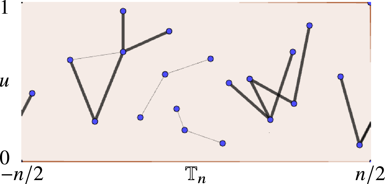
 ℓ=2
 Tn,T
 Tn,T=14

 Open access

