1. Introduction
Let X be a Lévy process with Lévy exponent
 $\kappa(\theta)= \log\mathbb{E} \mathrm{e}^{\theta X(1)}$
and define
 $\overline X(t)=\sup\{X(s)\colon s\le t\}$
,
 $\underline X(t)=\inf\{X(s)\colon s\le t\}$
. Also let
 $e_\eta$
be an independent exponentially distributed time, written as
 $e_\eta \sim \operatorname{Exp} (\eta)$
. The standard form of the Wiener–Hopf (WH) factorisation of X then states that
 $\overline X(e_\eta)$
and the displacement
 $D(e_\eta)=\overline X(e_\eta)-X(e_\eta)$
of
 $X(e_\eta)$
from the maximum are independent, and that
 $D(e_\eta)$
has the same distribution as
 $-\underline X(e_\eta)$
. In transform formulation, this gives the following factorisation of the moment generating function (m.g.f.) of
 $X(e_\eta)= \overline X(e_\eta) -(\overline X(e_\eta)-X(e_\eta))$
:
 \begin{equation} \mathbb{E}\mathrm{e}^{\theta X(e_\eta)} = \int_0^\infty \mathrm{e}^{t\kappa(\theta)}\eta\mathrm{e}^{-\eta t}\,\mathrm{d}t = \frac{\eta}{\eta-\kappa(\theta)} = \mathbb{E}\mathrm{e}^{\theta \overline X(e_\eta)}\cdot \mathbb{E}\mathrm{e}^{\theta \underline X(e_\eta)},\end{equation}
which is valid at least for
 $\theta$
purely imaginary. In order for these results to be non-trivial, assume in the following that X is not a subordinator, since in that case
 $\overline X(e_\eta)=X(e_\eta)$
and
 $\underline X(e_\eta)=0$
.
For the simplest case, where X is a Brownian motion BM
 $(\mu,\sigma^2)$
,
 $\overline X(e_\eta)$
and
 $-\underline X(e_\eta)$
are exponentially distributed with respective rates
 $\rho_+$
and
 $\rho_-$
, where
 \begin{equation*} \rho_{\pm} = \mp\frac{\mu}{\sigma^2}+\sqrt{\frac{\mu^2}{\sigma^4}+\frac{2\eta}{\sigma^2}}.\end{equation*}
The main case beyond BM that has been considered in the literature is when the jumps of X in one or both directions are phase-type (PH; see below) or, more generally, are matrix-exponential (ME), which is equivalent to the Laplace transform being rational (the ratio of polynomials). An often-cited paper in that vein is [Reference Lewis and Mordecki25], but there are earlier references [Reference Asmussen, Avram and Pistorius7, Reference Avram, Pistorius and Usabel9, Reference Mordecki26]. Among the many papers on WH factorisation in this setting, and covering related problems and extensions, we mention in particular [Reference Asmussen3, Reference Asmussen and Ivanovs8, Reference Bladt and Ivanovs10, Reference Ivanovs17–Reference Jiang and Pistorius19, Reference Kuznetsov22, Reference Kuznetsov, Kyprianou, Pardo and Van Schaik23, Reference Mordecki27, Reference Pistorius28]. The solutions in the majority of these references are expressed in terms of the roots of the equation
 $\kappa^*(\theta)=\eta$
, where
 $\kappa^*$
is an approriate analytic continuation of the Lévy exponent. This equation involves polynomials and the location of the roots by means of Rouché’s theorem. Beyond the BM or PH/ME setting, there are some specialised WH examples in [Reference Hackmann15, Reference Kuznetsov20, Reference Kuznetsov21, Reference Kuznetsov, Kyprianou, Pardo and Van Schaik23, Reference Kuznetsov and Peng24].
The main result of the present paper is a different representation of the distribution of
 $\overline X(e_\eta)$
. More precisely, we assume throughout that the jumps of X in the positive direction follow a compound Poisson (CP) process Y(t) with Poisson rate
 $\lambda$
and jumps which are PH or, more generally, ME. We can then write
 \begin{align} X(t) = Y(t)+Z(t) = \sum_{i=1}^{N(t)}V_i+Z(t),\end{align}
where Z is spectrally negative, with Lévy exponent say
 $\kappa_Z$
, N is a Poisson
 $(\lambda)$
process,
 $V_1,V_2,\ldots$
the upward jumps, and where obvious independence assumptions apply. The result is that
 $\overline X(e_\eta)$
is again PH/ME with computable parameters. This presents a structural property of
 $\overline X(e_\eta)$
and leads to matrix expressions like
 $f_{\overline X(e_\eta)}(x) = \boldsymbol{\gamma}\mathrm{e}^{\boldsymbol{G}x}\boldsymbol{g}$
,
 $\mathbb{P}(\overline X(e_\eta)\le x) = 1-\boldsymbol{\gamma}\mathrm{e}^{\boldsymbol{G}x}\boldsymbol{1}$
, and
 $\mathbb{E}\mathrm{e}^{\theta\overline X(e_\eta)} = \boldsymbol{\gamma}({-}\theta \boldsymbol{I}-\boldsymbol{G})^{-1}\boldsymbol{g}$
for the probability density function (p.d.f.), cumulative distribution function (c.d.f.), and m.g.f. of
 $\overline X(e_\eta)$
which are much more compact than the root expansions. Here,
 $f_Y$
denotes the density of a random variable (r.v.) Y and
 $\boldsymbol{1}$
is the column vector with all components equal to 1. Further,
 $\boldsymbol{\gamma}$
is a row vector,
 $\boldsymbol{g}$
a column vector, and
 $\boldsymbol{G}$
a square matrix, all of which are computable by algorithms to be presented. In addition, the iterative form of the algorithms has proved less sensitive to the curse of dimension than the root-finding ones, as remarked, for example, in [Reference Ivanovs17]. Note also that root-finding in high dimensions is often formulated as an eigenvalue problem, solved by iteration.
An argument in favour of considering only the PH setting is that our proofs are probabilistic rather than analytic/algebraic as in the ME case and that methods for fitting PH distributions [Reference Bladt and Nielsen11, Chapter 13] are far better developed than for the ME case. In view of this, we start by considering the PH case in Section 4. A numerical example is presented in Section 5. In addition to illustrating the general WH results, the example also shows how PH approximations may be performed. The ME case is treated in Section 6; the extension from PH to ME can be motivated by the fact that the dimensions of matrices, vectors, etc. can be substantially reduced in some cases and that there are examples of distributions that are ME but not PH (nevertheless, both classes are dense). In both cases, it turns out that we need to distinguish between two cases according to whether
 $-Z$
is a subordinator or not (this distinction also occurs in the classical algorithms, where the number of roots is different in the two cases). This determines whether Z can attain strictly positive values, both for some
 $t>0$
on the whole line and in a neighbourhood of
 $t=0$
. The subordinator case comprises the important case where both upward and downward jumps are CP/ME and no drift or Brownian parts are present. First, some preliminaries are given in Section 2.
2. Preliminaries
We start by recapitulating a few basic facts about PH distributions. The underlying object is a terminating Markov process
 $\{J(t)\}_{t<\zeta}$
on the finite phase space
 $E= \{1,\ldots,p\}$
(or any other set with p elements), having transition rates
 $t_{ij}$
for
 $i\ne j$
, killing rate of
 $t_i\geq 0$
in state i, with
 $t_{ii}$
then being defined by
 $t_{ii}=-\sum_{j\ne i}t_{ij}-t_{i}$
, and initial probabilities
 $\alpha_i=\mathbb{P}(J(0)=i)$
. We write
 $\boldsymbol{T}$
for the matrix
 $(t_{ij})_{i,j\in E}$
,
 $\boldsymbol{t}$
for the column vector
 $(t_1\,\cdots\,t_p)^\top$
, and
 $\boldsymbol{\alpha}$
for the row vector
 $(\alpha_1\,\cdots\,\alpha_p)$
. Then
 $\boldsymbol{t}=-\boldsymbol{T}\boldsymbol{1}$
, where
 $\boldsymbol{1}= (1\,\cdots\, 1)^\top$
. The
 $\operatorname{PH}(\boldsymbol{\alpha},\boldsymbol{T})$
distribution is then the distribution of the lifetime
 $\zeta= \inf\{t\ge 0\colon J(t)\not\in E\}$
. This allows the distribution to have an atom of size
 $1-\boldsymbol{\alpha}\boldsymbol{1}$
at
 $x=0$
. When it is important to stress the dimension, we write
 $\operatorname{PH}_p(\boldsymbol{\alpha},\boldsymbol{T})$
.
The c.d.f. is
 $\mathbb{P}(\zeta\le x)=1-\boldsymbol{\alpha}\mathrm{e}^{\boldsymbol{T}x}\boldsymbol{1}$
, the p.d.f. is
 $\boldsymbol{\alpha}\mathrm{e}^{\boldsymbol{T}x}\boldsymbol{t}$
, and the m.g.f. is
 $\mathbb{E}\mathrm{e}^{\theta\zeta}= \boldsymbol{\alpha}({-}\theta I-\boldsymbol{T})^{-1}\boldsymbol{t}$
. PH distributions form a dense set in the set of all distributions on
 $[0,\infty)$
, which, together with their underlying probabilistic structure and tractability, provides a strong motivation for their use. See further [Reference Bladt and Nielsen11, Chapter 3].
We will need a bit of functional calculus for matrices (see [Reference Bladt and Nielsen11, Section 3.4), for example a matrix version of a cumulant function. In examples with exponential moments in at least one direction (as is sufficient for our purposes), we have
 $\kappa(\theta)= \sum_1^\infty \kappa_n\theta^n/n!$
, where
 $\kappa_1,\kappa_2,\ldots$
are the cumulants, and may then define
 $\kappa(\boldsymbol{A})$
as
 $\sum_1^\infty \kappa_n\boldsymbol{A} ^n/n!$
. Computationally, and for other purposes, it may sometimes be more convenient to represent
 $\kappa(\boldsymbol{A})$
, and other analytic functions on the form
 $\varphi(\boldsymbol{A})$
(e.g. in Theorem 4.1), as the Cauchy integral
 \begin{equation} \varphi(\boldsymbol{A}) = \frac{1}{2\pi\mathrm{i}} \oint_C\varphi(z)(z\boldsymbol{I}-\boldsymbol{A})^{-1}\,\mathrm{d}z,\end{equation}
where all eigenvalues of
 $\boldsymbol{A}$
are inside the simple closed curve C.
Lemma 2.1. For an r.v. V with cumulant function
 $\ell(\theta)=\log\mathbb{E}\mathrm{e}^{\theta V}$
,
 $\mathbb{E}\mathrm{e}^{\boldsymbol{A}V}=\mathrm{e}^{\ell(\boldsymbol{A})}$
provided any eigenvalue
 $\rho$
of
 $\boldsymbol{A} $
is in the interior of the domain of
 $\ell$
. In particular, for a Lévy process X with Lévy exponent
 $\kappa$
,
 $\mathbb{E}\mathrm{e}^{\boldsymbol{A}X(t)} = \mathrm{e}^{t\kappa(\boldsymbol{A})}$
.
Proof. Since a Laplace transform is analytic wherever it is defined, (2.1) gives
 \begin{equation*} \mathbb{E}\mathrm{e}^{\boldsymbol{A}V} = \frac{1}{2\pi\mathrm{i}}\oint_C\mathbb{E}\mathrm{e}^{zV}(z\boldsymbol{I}-\boldsymbol{A})^{-1}\,\mathrm{d}z = \frac{1}{2\pi\mathrm{i}}\oint_C\mathrm{e}^{\ell(z)}(z\boldsymbol{I}-\boldsymbol{A})^{-1}\mathrm{d}z = \mathrm{e}^{\ell(\boldsymbol{A})}. \end{equation*}
The following lemma will serve as a check of the accuracy of our numerical computations in Section 5.
Lemma 2.2. Assume that
 $X\stackrel{\mathrm{d}}{=}-X$
. Then
 $\mathbb{V}\mathrm{ar} \overline X(e_\eta)=\mathbb{V}\mathrm{ar} X(1)/2\eta$
.
Proof. Let
 $Y=X(e_\eta)$
and
 $Z=\overline X(e_\eta)$
, with corresponding cumulant functions
 $\kappa_Y,\kappa_Z$
. Taking logarithms in (1.1) and using the symmetry property of X then gives
 $\kappa_Y(\theta) = \kappa_Z(\theta)+\kappa_Z(-\theta)$
. Differentiating twice and letting
 $\theta=0$
gives
 $\mathbb{V}\mathrm{ar}Y = \kappa''_Y(0) = 2\kappa''_Z(0) = 2\mathbb{V}\mathrm{ar}Z$
, but
 \begin{align*} \mathbb{V}\mathrm{ar} Y & = \mathbb{E}[\mathbb{V}\mathrm{ar}(X(e_\eta) \mid e_\eta)] + \mathbb{V}\mathrm{ar}[\mathbb{E}(X(e_\eta)\mid e_\eta)] \\ & = \mathbb{E}[e_\eta\cdot\mathbb{V}\mathrm{ar}X(1)] + \mathbb{V}\mathrm{ar}(e_\eta\cdot\mathbb{E}X(1)) = \mathbb{V}\mathrm{ar}X(1)/\eta+0. \end{align*}
In the following,
 $\omega_0$
will denote the time of the first jump of the CP/PH part and
 $\omega=\omega_0\wedge e_\eta$
.
3. The PH case with Z being a subordinator
Theorem 3.1. Assume in 1.2 that the
 $V_i\sim \operatorname{PH}_p(\boldsymbol{\alpha},\boldsymbol{T})$
, and that
 $-Z$
is a subordinator. Then the distribution of
 $\overline X(e_\eta)$
consists of an atom at 0 of size
 $1-\boldsymbol{\beta}\boldsymbol{1}$
, and an absolute continuous part which is
 $\operatorname{PH}_p(\boldsymbol{\beta},\boldsymbol{G}(\boldsymbol{\beta}))$
distributed. Here,
 $\boldsymbol{G}(\boldsymbol{\beta})=\boldsymbol{T}+\boldsymbol{t}\boldsymbol{\beta}$
, where
 $\boldsymbol{\beta}$
solves
 $\boldsymbol{\beta}=\psi(\boldsymbol{\beta})$
with
 $\psi(\boldsymbol{\beta}) = \lambda\boldsymbol{\alpha} ((\lambda+\eta)\boldsymbol{I}-\kappa_Z(-\boldsymbol{G}(\boldsymbol{\beta})))^{-1}$
. The row vector
 $\boldsymbol{\beta}$
can be computed by iteration,
 $\boldsymbol{\beta}^{(n)}\uparrow\boldsymbol{\beta}$
, where
 $\boldsymbol{\beta}^{(n)}=\psi\bigl(\boldsymbol{\beta}^{(n-1)}\bigr)$
and
 $\boldsymbol{\beta}^{(0)}=\boldsymbol{0}$
.
Note that the eigenvalue assumptions of Lemma 2.1 are fulfilled to make
 $\kappa_Z(-\boldsymbol{G}(\boldsymbol{\beta}))$
well-defined:
 $\boldsymbol{G}(\boldsymbol{\beta})$
will be seen to be the generator of a terminating Markov process, hence all eigenvalues have strictly negative real part, and
 $\kappa_Z(\theta)$
is well-defined whenever
 $\Re(\theta)\ge 0$
.
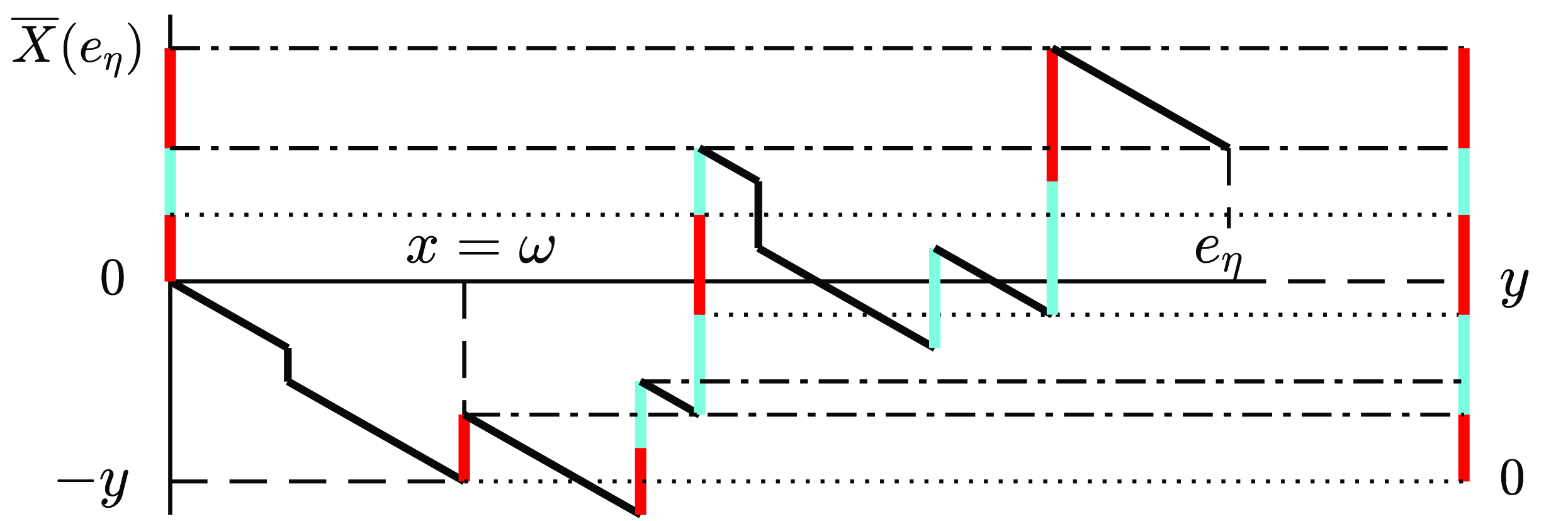
Proof. The intuition underlying our analysis is illustrated in Figure 1. Here, Z is taken as a sum of a negative drift and CP negative jumps, and the phase space E is given by
 $E=\{$
red, cyan
 $\}$
. We then construct a terminating Markov process
 $\xi$
on the vertical axis with the same state space. The process initiates at 0 when the first jump (if at all) upcrosses the horizontal axis, by projecting the underlying Markov process, which generates the jump onto the left vertical axis. Upon termination of the jump, the construction is repeated relative to the new running maximum: the next time a jump upcrosses the current maximum level, the Markov jump process underlying Markov process from the overshoot is projected onto the (left) vertical axis, and thereby concatenated with the part relating to the first overshoot. In the figure, this happens when the vertical Markov process from a jump crosses a dotted line in
 $(0,\infty)$
.
The case where
 $-Z$
is a subordinator.

The process
 $\xi$
has two types of transition
 $i\to j$
. The first ones correspond to jumps in the CP process occurring at rate
 $t_{ij}$
and are marked with a dotted horizontal line. In Figure 1 there is just one of this type, the first from red to cyan. The second ones, marked with a dash-dotted horizontal line, occur at the top of a jump (rate
 $t_i$
) and are reset according to a certain probability
 $\beta_j<1$
. In Figure 1, the first is the transition cyan to red, while there is no resetting on the top of the jump leading to
 $\overline X(e_\eta)$
. Therefore, the total generator is
 $\boldsymbol{T}+\boldsymbol{t}\boldsymbol{\beta}$
, where
 $\boldsymbol{\beta}=(\beta_1\,\cdots\,\beta_p)$
is also the initial vector for
 $\xi$
. The remaining problem is to compute
 $\boldsymbol{\beta}$
.
To prove that
 $\boldsymbol{\beta}=\psi(\boldsymbol{\beta})$
, we condition on the value
 $-y$
of Z just before the first upward jump of Y (in the red phase in the figure), occurring before
 $e_\eta$
at time
 $x=\omega$
at rate
 $\lambda\mathrm{e}^{-(\lambda+\eta)x}$
; cf. Lemma 4.1(i). We now construct a second terminating Markov jump process,
 $\xi^\prime$
, by shifting the origin (0,0) to
 $(x,-y)$
, cf. the dashed horizontal line. Next, we project the underlying Markov processes from the jumps onto the vertical axis in exactly the same way as for
 $\xi$
. This axis containing
 $\xi'$
is shown on the right of the figure and has a zero marked at the original level
 $-y$
, and we have used the same convention for dotted and dash-dotted lines as for
 $\xi$
.
The right vertical process
 $\xi^\prime$
is then again Markov with generator
 $\boldsymbol{G}(\boldsymbol{\beta})$
, though its initial distribution is
 $\boldsymbol{\alpha}$
rather than
 $\boldsymbol{\beta}$
. Then
 $\boldsymbol{\beta}$
, the initial distribution for
 $\xi$
, is precisely its state vector
 $\boldsymbol{\alpha}\mathrm{e}^{\boldsymbol{G}(\boldsymbol{\beta})y}$
, the distribution of
 $\xi^\prime$
at time y. It follows from Lemma 2.1 that
 \begin{align} \boldsymbol{\beta} & = \boldsymbol{\alpha}\int_0^\infty\lambda\mathrm{e}^{-(\lambda+\eta)x} \mathbb{E}\mathrm{e}^{\boldsymbol{G}(\boldsymbol{\beta})(-Z(x))}\,\mathrm{d}x \\ & = \boldsymbol{\alpha}\int_0^\infty\lambda \exp\{-(\lambda+\eta)\boldsymbol{I} x+\kappa_Z(-\boldsymbol{G}(\boldsymbol{\beta}))x\}\,\mathrm{d}x = \psi(\boldsymbol{\beta}). \end{align}
The argument for
 $\boldsymbol{\beta}^{(n)}\uparrow \boldsymbol{\beta}$
is essentially the same as in [Reference Asmussen1], [Reference Asmussen2, pp 241–242], or [Reference Bladt and Nielsen11, pp. 373–375]. We add here that the monotonicity of the iteration follows from (3.1) since
 $-Z(x)\ge 0$
and
 $\mathrm{e}^{\boldsymbol{G}(\boldsymbol{\beta})x}$
is non-decreasing in
 $\boldsymbol{\beta}$
. This last fact is not obvious from the series representation of the matrix exponential function since
 $\boldsymbol{G}(\boldsymbol{\beta})$
, and hence possibly the
 $\boldsymbol{G}(\boldsymbol{\beta})^n$
, contains negative elements. However, it may be seen from the uniformity representation, cf. [Reference Bladt and Nielsen11, pp. 51ff], since the matrix
 $\boldsymbol{I}+\boldsymbol{G}(\boldsymbol{\beta})/a$
, and hence its powers, only contain non-negative elements for sufficiently large a.
Example 3.1. If Z is CP with Poisson rate
 $\lambda_-$
and generic jump
 $\zeta_-<0$
, then
 $\kappa_Z(\theta) = \lambda_-(\mathbb{E}\mathrm{e}^{\theta\zeta_-}-1)$
and
 $\kappa_Z(-\boldsymbol{G}) = \lambda_-(\mathbb{E}\mathrm{e}^{-\boldsymbol{G}\zeta_-}-\boldsymbol{I})$
. If
 $-\zeta_- \sim \operatorname{PH}(\boldsymbol{\alpha}_-,\boldsymbol{T}_-)$
, this last expression may be evaluated via
 \begin{align*} \mathbb{E}\mathrm{e}^{-\boldsymbol{G}\zeta_-} & = \int_0^\infty\boldsymbol{\alpha}_-\mathrm{e}^{\boldsymbol{T}_- x}\boldsymbol{t}_-\cdot \mathrm{e}^{\boldsymbol{G}x}\,\mathrm{d}x \\ & = \int_0^\infty\boldsymbol{\alpha}_-\mathrm{e}^{\boldsymbol{T}_- x}\boldsymbol{t}_-\cdot \boldsymbol{I}\mathrm{e}^{\boldsymbol{G}x}\boldsymbol{I}\,\mathrm{d}x \\ & = \int_0^\infty(\boldsymbol{\alpha}_-\otimes\boldsymbol{I})\mathrm{e}^{(\boldsymbol{T}_-\oplus\boldsymbol{G})x} (\boldsymbol{t}_-\otimes\boldsymbol{I})\,\mathrm{d}x = -(\boldsymbol{\alpha}_-\otimes\boldsymbol{I})(\boldsymbol{T}_-\oplus\boldsymbol{G})^{-1} (\boldsymbol{t}_-\otimes\boldsymbol{I}), \end{align*}
cf. [Reference Bladt and Nielsen11, Section A.4] for the Kronecker calculus. If
 $-\zeta_-$
is exponential
 $\mu$
, we simply have
 $\mathbb{E}\mathrm{e}^{-\boldsymbol{G}\zeta_-}= (\boldsymbol{I}-\boldsymbol{G}/\mu)^{-1}$
; this generalises straightforwardly to a mixture of exponentials or Erlangs.
4. The PH case with Z not a subordinator
We first remark that with positive values of Z occurring with positive probability, we are always in one of the situations where Z either (i) contains a Brownian component, and/or (ii) contains an infinite-variation jump component, or (iii) has the form
 $Z(t)=at+J(t)$
where
 $a>0$
and J is a finite-variation jump process with the Lévy measure concentrated on
 $(-\infty,0)$
.
The situation is illustrated in Figure 2, where the blue segments of the path of X between upward PH jumps are governed by Z. Downward jumps of Z are shown in green.
The case of Z taking positive values.

Since the first upward jump occurs at some strictly positive time, the path of X starts by such a segment attaining positive values immediately. Thus the state space of
 $\xi$
needs to be augmented with an extra state blue, denoted 0 in the following. The initial state of
 $\xi$
is always blue and is possibly followed by a sequence of the states in E coming from the PH jumps. Upon exit at the top of a jump,
 $\xi$
returns to the blue state.
Formally, we let
 $E_0=\{0\}\cup E= \{0,1,\ldots,p\}$
. For a
 $1\times (p+1)$
row vector
 $\boldsymbol{\beta}=(\beta_0\,\beta_1\,\cdots\ \beta_p)$
, we write
 $\boldsymbol{\beta}_{1:p}=(\beta_1\ \cdots \ \beta_p)$
. We also write
 $\boldsymbol{1}_0=(1\,0 \cdots0)$
for the
 $(p+1)$
-dimensional unit row vector.
The following lemma contains the key steps in our derivation of the distribution of
 $\overline X(e_\eta)$
. In part (i),
 $\widetilde X_{0:{T}}(t)=X(t\wedge T)$
denotes the process X being absorbed at time T at its running value X(T).
Lemma 4.1.
-
(i) Let
 $e(\lambda_1)\sim \operatorname{Exp}(\lambda_1)$
and
$e(\lambda_2)\sim \operatorname{Exp}(\lambda_2)$
be mutually independent and independent of X, and write
$e(\lambda_1+\lambda_2) = e(\lambda_1) \wedge e(\lambda_2)$
. Then for all measurable subsets A of the Skorokhod space
\begin{align*} \mathbb{P}\bigl(\widetilde X_{0:{e(\lambda_1)}}\in A,\, e(\lambda_1)< e(\lambda_2)\bigr) & = \mathbb{P}\bigl(\widetilde X_{0:{e(\lambda_1+\lambda_2)}}\in A\bigr) \cdot \mathbb{P}(e(\lambda_1) < e(\lambda_2)) \\ & = \frac{\lambda_1}{\lambda_1+\lambda_2}\mathbb{P}\bigl(\widetilde X_{0:{e(\lambda_1+\lambda_2)}}\in A\bigr) \end{align*}
$D[0,\infty)$
.
-
(ii)
$\kappa_Z(\theta)=\log\mathbb{E}\mathrm{e}^{\theta Z(1)}$
is well-defined for all
$\theta$
with real parts
$\Re(\theta)\in[0,\infty)$
and increases strictly monotonically from
$\min_{\theta\ge0}\kappa_Z(\theta) \le 0$
to
$+\infty$
as
$\theta\uparrow\infty$
. -
(iii) Conditionally on
$\omega<\mathrm{e}_\eta$
,
$\overline X(\omega\!-\!)=\overline Z(\omega) \sim \operatorname{Exp}(\delta)$
, where
$\delta$
is the unique positive solution of
$\kappa_Z(\delta)=\lambda+\eta$
. -
(iv) Define
$\varphi(\theta)=\mathbb{E}\mathrm{e}^{\theta D(\omega)}$
as the m.g.f. of the displacement
$D(\omega)=\overline X(\omega)-X(\omega)$
of
$X(\omega)$
from
$\overline X(\omega)$
given
$\omega < \mathrm{e}_\eta$
. Then
$\varphi(\theta)$
is well-defined for all
$\theta$
with
$\Re(\theta)\in(\!-\!\infty,0]$
and equals
$(1+\theta/\delta)/(1-\kappa_Z(-\theta)/(\lambda+\eta))$
.




Proof. For (i), we have
 $\mathbb{P}\bigl(\widetilde X_{0:{e(\lambda)}}\in A\bigr) = \int_0^\infty\mathbb{P}\bigl(\widetilde X_{0:{x}}\in A\bigr)\lambda\mathrm{e}^{-\lambda x}\,\mathrm{d}x$
. Similarly,
 \begin{align*} \mathbb{P}\bigl(\widetilde X_{0:{e(\lambda_1)}}\in A,\, e(\lambda_1)< e(\lambda_2)\bigr) & = \int_0^\infty\mathbb{P}\bigl(\widetilde X_{0:{x}}\in A,\,x< e(\lambda_2)\bigr) \lambda_1\mathrm{e}^{-\lambda_1 x}\,\mathrm{d}x \\ & = \int_0^\infty\mathbb{P}\bigl(\widetilde X_{0:{x}}\in A\bigr)\mathrm{e}^{-\lambda_2 x} \lambda_1\mathrm{e}^{-\lambda_1 x}\,\mathrm{d}x \\ & = \frac{\lambda_1}{\lambda_1+\lambda_2}\int_0^\infty\mathbb{P}\bigl(\widetilde X_{0:{x}}\in A\bigr) (\lambda_1+\lambda_2)\mathrm{e}^{-(\lambda_1+\lambda_2)x}\,\mathrm{d}x \\ & = \frac{\lambda_1}{\lambda_1+\lambda_2}\mathbb{P}\bigl(\widetilde X_{0:{e(\lambda_1+\lambda_2)}}\in A\bigr). \end{align*}
Part (ii) is just a well-known fact about spectrally negative Lévy processes, where
 $\psi(\theta)\to\infty$
as
 $\theta\uparrow\infty$
follows from the assumption of
 $-Z$
not being a subordinator so that
 $\mathbb{P}(Z(1)>0)>0$
. Also, (iii) is well known, but the proof is short, so we include it for completeness. First, it is probabilistically clear from the upward skip-free property of Z that the distribution of
 $\overline X(\omega)$
is memoryless, hence exponential for some
 $\delta$
. By (i), we treat
 $\omega$
as
 $\operatorname{Exp}(\lambda+\eta)$
-distributed, and (1.1) then gives
 \begin{equation} \frac{\lambda+\eta}{\lambda+\eta-\kappa_Z(\theta)} = \frac{\delta}{\delta-\theta}\mathbb{E}\mathrm{e}^{\theta\underline Z(\omega)}. \end{equation}
But
 $\mathbb{E}\mathrm{e}^{\theta\underline Z(\omega)}$
is finite and non-zero for all
 $\theta>0$
, so we must have
 $\kappa_Z(\delta)=\lambda+\eta$
.
Finally, in (iii),
 $D(\omega)>0$
implies
 $\varphi(\theta)$
is well-defined and analytic for all
 $\theta$
with
 $\Re(\theta)\in(\kern-3pt-\kern-2pt\infty,0]$
. The expression for
 $\varphi(\theta)$
in the region
 $\Re(\theta)\in(\kern-3pt -\kern-2pt \delta,0]$
then follows from (1.1), (4.1), and
 $D(\omega)=-\underline Z(\omega)$
. At
 $\theta=-\delta$
, both the numerator and denominator are zero but have non-zero derivatives, and for
 $\theta<-\mu$
, both are negative. The validity of the expression for
 $\varphi(\theta)$
for all
 $\theta$
with
 $\Re(\theta)\in(-\infty,0]$
thus follows by analytic continuation.
Theorem 4.1. Assume that the
 $V_i$
in (1.2) are
 $\operatorname{PH}_p(\boldsymbol{\alpha},\boldsymbol{T})$
and that
 $-Z$
is not a subordinator. Then
 $\overline X(e_\eta)\sim\operatorname{PH}_{p+1}(\boldsymbol{1}_0,\boldsymbol{G}(\boldsymbol{\beta}))$
on
 $(0,\infty)$
with phase space
 $E_0$
, initial vector
 $\boldsymbol{1}_0$
, and phase generator
 \[ \boldsymbol{G}(\boldsymbol{\beta}) = \left(\begin{array}{l@{\quad}l} -\delta(1-\beta_0) & \delta\boldsymbol{\beta}_{1:p} \\ \boldsymbol{t} & \boldsymbol{T} \end{array} \right). \]
Here,
 $\delta$
is the positive solution of
 $\kappa_Z(\delta)=\lambda+\eta$
, and
 $\boldsymbol{\beta}:1\times(p+1)$
solves
 $\boldsymbol{\beta}=\psi(\boldsymbol{\beta})$
where
 \[ \psi(\boldsymbol{\beta}) = \frac{\lambda}{\lambda+\eta}(0\,\,\boldsymbol{\alpha}) \varphi(\boldsymbol{G}(\boldsymbol{\beta})), \]
with
 $\varphi$
as in Lemma 4.1(iv).
The row vector
 $\boldsymbol{\beta}$
can be computed by iteration,
 $\boldsymbol{\beta}^{(n)}\uparrow \boldsymbol{\beta}$
where
 $\boldsymbol{\beta}^{(n)}=\psi\bigl(\boldsymbol{\beta}^{(n-1)}\bigr)$
and
 $\boldsymbol{\beta}^{(0)}=\boldsymbol{0}$
.
Proof. Let
 $\xi'$
be the
 $\xi$
-process on the right in Figure 2 and define
 $\boldsymbol{\beta}$
as the vector of state probabilities of
 $\xi'$
at its upcrossing of
 $\overline X(\omega)$
. We now use Lemma 4.1 with
 $e(\lambda_1)=\omega$
,
 $e(\lambda_2)=e_\eta$
. The event
 $\mathrm{e}_\eta<\omega$
gives no contribution to
 $\boldsymbol{\beta}$
, so we have to treat
 $\omega$
as Exp
 $(\lambda+\eta)$
. Thus by Lemma 4.1(iii),
 $\overline X(\omega)\sim\operatorname{Exp}(\delta)$
, where
 $\delta$
is as stated. However, the
 $\xi$
-process on the left may return immediately to the blue state 0, which occurs with probability
 $\beta_0$
(an example of such a backcoupling is in the last blue segment of
 $\xi$
in Figure 2). Thus, the exit rate of
 $\xi$
from state 0 is
 $\delta(1-\beta_0)$
, which gives the upper left entry of the
 $\boldsymbol{G}(\boldsymbol{\beta})$
matrix. The forms of the remaining entries are evident.
The process
 $\xi'$
has initial distribution
 $(0\quad\boldsymbol{\alpha})$
and has to traverse the distance
 $D=D(\omega)$
to upcross
 $\overline X(\omega)$
, but only starts if
 $\omega < e_\eta$
. Thus
 \[ \boldsymbol{\beta} = \mathbb{P}(\omega < e_\eta)(0\quad\boldsymbol{\alpha})\mathbb{E}\mathrm{e}^{\xi'(D(\omega))} = \frac{\lambda}{\lambda+\eta}(0\quad\boldsymbol{\alpha})\varphi(\boldsymbol{G}(\boldsymbol{\beta})). \]
That
 $\boldsymbol{\beta}^{(n)}\uparrow \boldsymbol{\beta}$
follows by similar reasoning to the proof of Theorem 3.1.
5. Numerical example
The traditional way to approximate the positive jumps would be to truncate the density n(x) of the Lévy measure
 $\nu$
to
 $(\varepsilon,\infty)$
for some small
 $\varepsilon$
and use the CP model with
 $\lambda=\int_\varepsilon^\infty n(x)\,\mathrm{d}x$
and density
 $h(x)= n(x)/\lambda$
,
 $x> \varepsilon$
, of the jumps (possibly, this would be supplemented by some approximation of the contribution from jumps in
 $(0,\varepsilon)$
). In the PH setting, we would then use some PH fit of h. This has, however, the disadvantage that distributions with sharp jumps, such as that of h(x) from
 $h(\varepsilon\!-\!)=0$
to
 $h(\varepsilon)=n(\varepsilon)/\lambda>0$
, require a huge number of phases to give a reasonable fit.
Instead, we use the completely monotone structure present in most of the standard examples [Reference Hackmann and Kuznetsov16] where
 \begin{equation} n(x) = \int_0^\infty\mathrm{e}^{-tx}v(t)\,\mathrm{d}t,\quad x>0,\end{equation}
for some function
 $v\ge 0$
on
 $(0,\infty)$
(and similarly for n(x),
 $x<0$
). That is, n(x) is a mixture of
 $\operatorname{Exp}(t)$
distributions, with respective weights
 $v(t)/t$
. In [Reference Hackmann and Kuznetsov16], this structure is used to approximate the upward jumps via Padé approximations. This leads to a scheme with the special structure of the PH jumps being hyperexponential (mixtures of exponentials); this is, of course, natural in view of (5.1).
Specifically, we considered a symmetric (
 $G=M$
) Carr–Geman–Madan–Yor (CGMY) (tempered stable) process with Lévy density
 $C\mathrm{e}^{-M|x|}/|x|^{Y+1}$
,
 $-\infty < x < \infty$
, [Reference Carr, Geman, Madan and Yor13]. Such a process can be written as
 $X=X^{\mathrm(u)}-X^{\mathrm(d)}$
, where
 $X^{\mathrm(u)}$
and
 $X^{\mathrm(d)}$
are independent spectrally positive CGMY processes both having Lévy densities
 $C\mathrm{e}^{-Mx}/x^{Y+1}$
,
 $x>0$
, and Lévy exponents
 \[\kappa^{(\mathrm{u})}(\theta)=\kappa^{(\mathrm {d})}(\theta)=C\Gamma(\!-\!Y)((M-\theta)^Y-M^Y).\]
We took the variance of X(1) to be 1 and the kurtosis to be
 $K=4$
. According to [Reference Asmussen4], such a process exists for any
 $Y\in(0,2)$
, and we took
 $Y=3/2$
corresponding to the infinite-variation case. Then the formulas of [Reference Asmussen4] give
 \[ M = \frac{1}{K^{1/2}}\sqrt{(2-Y)(3-Y)} = 0.433, \qquad C = \frac{1}{2\Gamma(2-Y)}M^{2-Y} = 0.186.\]
It is an easy consequence of the integral representation of the gamma function that the Lévy density
 $C\mathrm{e}^{-Mx}/x^{Y+1}$
of the positive jumps is completely monotone corresponding to
 $v(t)=C(t-M)^Y/\Gamma(Y+1)$
,
 $t>M$
. The relevant Padé approximations from [Reference Hackmann and Kuznetsov16] are the
 $[n+1/1]$
and
 $[n+2/2]$
ones in Proposition 2 there. We use the
 $[n+1/1]$
one, where the approximation of
 $\kappa^{(\mathrm{u})}\theta)$
is given as
 \begin{equation} \widehat\kappa^{(\mathrm{u})}_n(\theta) = \frac{P(\theta)}{Q(\theta)} = a\theta+\sum_{i=1}^n\lambda_i\bigg( \frac{\mu_i}{\mu_i-\theta}-1\bigg)\end{equation}
for certain polynomials P,Q of degree
 $n+1$
(respectively n), and certain a,
 $\lambda_1,\ldots,\lambda_n>0$
,
 $\mu_1,\ldots,\mu_n>0$
. The last expression is a slight rewriting of [Reference Hackmann and Kuznetsov16, (25)], but the key observation leading to the equivalence is that
 \[ \int_0^\infty(\mathrm{e}^{\theta x}-1-\theta x)\mu\mathrm{e}^{-\mu x}\,\mathrm{d}x = \frac{\mu}{\mu-\theta}-1-\frac{\theta}{\mu} = \frac{\theta^2/\mu}{\mu-\theta} .\]
The last expression in (5.2) is the Lévy exponent of a hyperexponential Lévy process with jumps arriving at rate
 $\lambda=\sum_1^n\lambda_i$
and being distributed as the mixture of n exponential distributions, with rate
 $\mu_i$
and weight
 $\lambda_i/\lambda$
for the ith. To this is added a linear drift at rate a. Computationally, we used the linear equations for the coefficients of Q (e.g. the Appendix in [Reference Hackmann and Kuznetsov16] or [Reference Weisstein29]) to get
 $\mu_1,\ldots,\mu_n$
as the roots of Q. Since the
 $[n+1/n]$
Padé approximation preserves the first
 $2n+2$
cumulants, we could then first get
 $\lambda_1,\ldots,\lambda_n$
as solutions of the linear equations
 \[ \int_0^\infty x^kn(x)\,\mathrm{d}x = C\Gamma(\!-\!Y)Y\cdots(Y\!-k+1)M^{Y-k} = \sum_{i=1}^n\frac{k!}{\mu_i^k}\lambda_i, \quad k=2,\ldots,n+1,\]
and next compute a as
 $C\Gamma(\!-\!Y)YM^{Y-1}-\sum_1^n\lambda_i/\mu_i$
. The Z process becomes
 $Z(t)=at-X^{\mathrm(d)}(t)$
.
We took
 $n=4,6,8,10$
and computed
 $\varphi(\boldsymbol{G})$
via diagonalisation. The iteration was stopped at
 $\overline m = \inf\bigl\{m\colon\big\|\boldsymbol{\beta}^{(m)}-\boldsymbol{\beta}^{(m-1)}\big\|<10^{-8}\bigr\}$
, which required
 $\overline m= 43$
, 69, 97, and 127 in the four cases. The program ran in just a few seconds on a 2022 MacBook Air. Graphical illustrations are given in Figure 3.
(a) Exact Lévy exponent
 $\kappa^{(\mathrm{u})}(\theta)$
and Padé approximations
 $\widehat\kappa^{(\mathrm{u})}_n(\theta)$
. (b) Approximated density of
 $\overline X(e_\eta)$
computed via the hyperexponential Padé scheme and Theorem 4.1.

As a check, we used Lemma 2.2 and the computed variances of the approximated PH distribution of
 $\overline X(e_\eta)$
, which were 0.500 34, 0.500 07, 0.500 02, and 0.500 01, to be compared with the exact value of 0.500 00. All of the above confirms the expected increase in accuracy as n increases. As an example of the numerical values of the parameters, the computations for
 $n=8$
gave
 \begin{gather*} \delta=207.2, \qquad a=-5.18, \\ \lambda_1,\ldots,\lambda_8=234.9,\,26.68,\,0.290,\,0.057,\,0.136,\,0.0032,\,6.2\times10^{-4},\,6.2\times10^{-5}, \\ \boldsymbol{\beta} = \bigl(0.165\ \ 0.740\ \ 0.036\ \ 0.0067\ \ 0.0017\ \ 4.7\times10^{-4}\ \ 1.2\times10^{-4}\ \ 2.4\times10^{-5}\ \ 2.5\times10^{-6}\bigr), \\ \boldsymbol{G} = \begin{pmatrix} -172.9 & 153.2 & 7.52 & 3.96 & 3.53 & 0.096 & 0.025 & 0.0050 & 0.0005 \\ 56.65 & -56.65 & 0 & 0 & 0 & 0 & 0 & 0 & 0 \\ 6.42 & 0 & -6.42 & 0 & 0 & 0 & 0 & 0 & 0 \\ 2.41 & 0 & 0 & -2.41 & 0 & 0 & 0 & 0 & 0 \\ 1.31 & 0 & 0 & 0 & -1.31 & 0 & 0 & 0 & 0 \\ 0.861 & 0 & 0 & 0 & 0 & -0.861 & 0 & 0 & 0 \\ 0.641 & 0 & 0 & 0 & 0 & 0 & -0.641 & 0 & 0 \\ 0.524 & 0 & 0 & 0 & 0 & 0 & 0 & -0.524 & 0 \\ 0.461 & 0 & 0 & 0 & 0 & 0 & 0 & 0 & -0.461 \\ \end{pmatrix}\end{gather*}
(where, obviously,
 $\mu_1, \ldots, \mu_8$
are the last eight elements of the first column of
 $\boldsymbol{G}$
).
Altogether, we take the results of this example as strong support for the usefulness of both our WH scheme and the Padé approximation.
Remark 5.1. Note that our implementation of the Padé approximation is fairly primitive, and more sophisticated methods involving double or multiple precision would be required to get much beyond
 $n=10$
.
An alternative allowing much higher n is a truncation scheme where the integral in (5.1) is cut off at some
 $A<\infty$
and the reduced part
 $\int_0^A\mathrm{e}^{-tx}v(t)\,\mathrm{d}t$
of n(x) coming from this is scaled to be a distribution. This is then fitted to a general PH distribution using maximum likelihood (which is typically implemented via the EM algorithm, [Reference Bladt and Nielsen11, Chapter 13]). The idea behind this is somewhat similar to that in the
 $\varepsilon$
scheme above, in the sense of disregarding ‘small’ jumps in the setting of (5.1), meaning those coming from a large t. We then approximate
 $X^{\mathrm(u)}$
by the contribution
 $X^{\mathrm(u)}_{0:A}$
from jumps coming from some
 $t<A$
in (5.1), to which we add some approximation
 $\widehat X^{(u)}_{A:\infty}$
to the contribution
 $X^{\mathrm(u)}_{A:\infty}$
from jumps coming from some
 $t\ge A$
. This scheme has been considered for simulation purposes in [Reference Asmussen5]. The simulation aspect is not relevant here, but we could use the observation from [Reference Asmussen5] that taking
 $\widehat X^{(u)}_{A:\infty}$
as BM can be justified by a limit theorem (actually, taking
 $\widehat X^{(u)}_{A:\infty}$
as a gamma process was observed to be somewhat more precise but is not relevant here since it would add some non-PH upward jumps). In view of the success of the Padé approximation in our example, we have not implemented this scheme.
6. Extension to matrix-exponentially distributed jumps
We now consider the same model as in Theorem 4.1, but we replace the distributional assumption of the upward jumps being of PH type by assuming that they follow the more general matrix-exponential (ME) distribution, written as
 $\operatorname{ME}(\boldsymbol{\alpha},\boldsymbol{T},\boldsymbol{t})$
(if we need to stress the dimension of the matrices and vectors, we write
 $\operatorname{ME}_p(\boldsymbol{\alpha},\boldsymbol{T},\boldsymbol{t})$
). This means that the upward jumps have a density of the form
 $f(x) =\boldsymbol{\alpha} \mathrm{e}^{\boldsymbol{T} x}\boldsymbol{t}$
, whereas for the PH type case we may take
 $\boldsymbol{t}=-\boldsymbol{T}\boldsymbol{1}$
. Here, the matrix
 $\boldsymbol{T}$
does not need to have the form of a sub-intensity matrix, and
 $\boldsymbol{\alpha}$
is not a (sub-)probability vector (e.g. it may contain negative values). In the ME terminology,
 $\boldsymbol{\alpha}$
is referred to as the starting vector,
 $\boldsymbol{T}$
as the generator, and
 $\boldsymbol{t}$
as the closing vector. However, we can always find a representation for which
 $\boldsymbol{t}=-\boldsymbol{T}\boldsymbol{1}$
, in which case the mass of the distribution is given by
 $\boldsymbol{\alpha}\boldsymbol{1}$
, whereas before
 $\boldsymbol{1}$
is the vector of ones.
In the PH case,
 $\boldsymbol{\alpha}$
is always chosen as the vector of initial probabilities for the underlying Markov process and
 $\boldsymbol{T}$
as the rate matrix. In the ME case, there is no such obvious choice, and many representations
 $(\boldsymbol{\alpha},\boldsymbol{T},\boldsymbol{t})$
of the same distribution are possible, sometimes creating a need for regularity assumptions. In particular, dimensionality becomes an issue, and the assumption we shall need is condition (R) from [Reference Bladt and Nielsen11, pp. 215ff]. For a representation ME
 $_q(\boldsymbol{\gamma},\boldsymbol{G},\boldsymbol{g})$
, it states that
 $\boldsymbol{g},\boldsymbol{G}\boldsymbol{g},\ldots,\boldsymbol{G}^{q-1}\boldsymbol{g}$
are linearly independent. It implies that if ME
 $_q(\boldsymbol{\gamma}^*,\boldsymbol{G},\boldsymbol{g})$
is also a representation, then
 $\boldsymbol{\gamma}^*=\boldsymbol{\gamma}$
. Any ME has some representation satisfying (R). For these and other facts on ME distributions used without detailed reference in the following, see [Reference Bladt and Nielsen11, Chapter 4].
We shall repeatedly use the representation
 \begin{align*} (\boldsymbol{\alpha}_1\,\,\boldsymbol{0}), \qquad \left(\begin{array}{l@{\quad}l} {\boldsymbol{S}}_1 & {\boldsymbol{s}}_1\boldsymbol{\alpha}_2 \\ \boldsymbol{0} & {\boldsymbol{S}}_2 \end{array} \right), \qquad \begin{pmatrix} (1-\boldsymbol{\alpha}_2\boldsymbol{1}){\boldsymbol{s}}_1 \\ {\boldsymbol{s}}_2 \end{pmatrix} \end{align*}
for the sum
 $U_1+U_2$
of two independent (possibly defective) r.v.s
 $U_1\sim \mathrm{ME}_{p_1}(\boldsymbol{\alpha}_1,{\boldsymbol{S}}_1,{\boldsymbol{s}}_1)$
,
 $U_2\sim\mathrm{ME}_{p_2}(\boldsymbol{\alpha}_2,{\boldsymbol{S}}_2,{\boldsymbol{s}}_2)$
(slighly adapted from [Reference Bladt and Nielsen11, p. 228]).
We shall give a detailed derivation of the following analogue of Theorem 4.1 and only at the end state the simpler parallel of Theorem 3.1.
Theorem 6.1.
Assume that
 $X(t)=Y(t)+Z(t)$
, where
 $-Z$
is not a subordinator and Y is CP
 $(\lambda,H)$
with H being
 $\operatorname{ME}_p(\boldsymbol{\alpha},\boldsymbol{T},\boldsymbol{t})$
with
 $\boldsymbol{t}=-\boldsymbol{T}\boldsymbol{1}$
and satisfying (R). Then
 $\overline X(e_\eta)$
isME
 $_{p+1}(\boldsymbol{1}_0,\boldsymbol{G}(\boldsymbol{\beta}),\boldsymbol{g}(\boldsymbol{\beta}))$
on
 $(0,\infty)$
with starting vector
 $\boldsymbol{1}_0=(1\ \ \ \boldsymbol{0}_{1:p})$
, and generator
 $\boldsymbol{G}(\boldsymbol{\beta})$
and closing vector
 $\boldsymbol{g}(\boldsymbol{\beta})$
given by
 \[ \boldsymbol{G}(\boldsymbol{\beta}) = \left(\begin{array}{l@{\quad}l} -\delta(1-\beta_0) & \delta\boldsymbol{\beta}_{1:p} \\ \boldsymbol{t} & \boldsymbol{T} \end{array} \right), \qquad \boldsymbol{g}(\boldsymbol{\beta}) = -\boldsymbol{G}(\boldsymbol{\beta})\boldsymbol{1} = \begin{pmatrix} \delta(1-\boldsymbol{\beta}\boldsymbol{1}) \\ \boldsymbol{0} \end{pmatrix}. \]
Here,
 $\delta$
is the positive solution of
 $\kappa_Z(\delta)=\lambda+\eta$
, and
 $\boldsymbol{\beta}\,:\,1\times(p+1)$
solves
 $\boldsymbol{\beta}=\psi(\boldsymbol{\beta})$
where
 \[ \psi(\boldsymbol{\beta}) = \frac{\lambda}{\lambda+\eta}(0\ \ \ \ \boldsymbol{\alpha}) \varphi(\boldsymbol{G}(\boldsymbol{\beta})), \]
with
 $\varphi$
as in Lemma 4.1(iv).
The row vector
 $\boldsymbol{\beta}$
can be computed by iteration,
 $\boldsymbol{\beta}^{(n)}\to \boldsymbol{\beta}$
as
 $n\rightarrow \infty$
, where
 $\boldsymbol{\beta}^{(n)}=\psi\bigl(\boldsymbol{\beta}^{(n-1)}\bigr)$
with
 $\boldsymbol{\beta}^{(0)}=\boldsymbol{0}$
.
Note that in contrast to the PH case, the convergence
 $\boldsymbol{\beta}^{(n)}\to \boldsymbol{\beta}$
need not be monotone, which is one of the reasons that the proof is substantially more involved in the ME case.
The proof is based on random walk theory in the presence of ME components. We start with a number of auxiliary results.
Lemma 6.1. If, for all
 $x\geq 0$
,
 $f_\beta(x)=\boldsymbol{\beta}\mathrm{e}^{\boldsymbol{S}x}\boldsymbol{s} \leq \boldsymbol{\gamma}\mathrm{e}^{\boldsymbol{S}x}\boldsymbol{s} = f_\gamma(x)$
are defective ME densities, then also
 $\boldsymbol{\alpha}\mathrm{e}^{(\boldsymbol{S}+\boldsymbol{s}\boldsymbol{\beta})t}\mathrm{e}^{\boldsymbol{S}x}\boldsymbol{s} \leq \boldsymbol{\alpha}\mathrm{e}^{(\boldsymbol{S}+\boldsymbol{s}\boldsymbol{\gamma})t}\mathrm{e}^{\boldsymbol{S}x}\boldsymbol{s}$
for all
 $x\geq 0$
.
Proof. An induction argument immediately implies that
 $f_\beta^{\ast n}(x) \leq f_\gamma^{\ast n}(x)$
for all
 $x\geq 0$
and all n. Hence, the corresponding renewal densities also satisfy
 \[ u_\beta(x) = \Bigg(f_0\ast\sum_{n=1}^\infty f_\beta^{\ast n}\Bigg)(x) \leq \Bigg(f_0\ast\sum_{n=1}^\infty f_\gamma^{\ast n}(x)\Bigg) = u_\gamma(x), \]
where
 $f_0(x)=\boldsymbol{\alpha}\mathrm{e}^{\boldsymbol{S}x}\boldsymbol{s}$
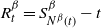
denotes the delay density. Given a time t, denote the residual lifetimes
 $R^\beta_t=S^\beta_{N^\beta(t)}-t$
and
 $R^\gamma_t=S^\gamma_{N^\gamma (t)}-t$
, where
 $N^\beta$
and
 $N^\gamma$
denote the corresponding delayed and terminating (defective) renewal processes with respective interarrival densities
 $f_\beta$
and
 $f_\gamma$
and delay density
 $f_0$
. Then
 \begin{align*} f_{R^{\beta}_t}(x) & = \boldsymbol{\alpha}\mathrm{e}^{\boldsymbol{S}(t+x)}\boldsymbol{s} + \int_0^{t}f_\beta(x+t-z)u_\beta(z)\,\mathrm{d}{z} \\ & \leq \boldsymbol{\alpha}\mathrm{e}^{\boldsymbol{S}(t+x)}\boldsymbol{s} + \int_0^{t}f_\gamma(x+t-z)u_\gamma(z)\,\mathrm{d}{z} = f_{R^{\gamma}_t}(x) \end{align*}
for all
 $x\geq 0$
. But then, by [Reference Bladt and Nielsen11, Theorem 5.7.5],
 $\boldsymbol{\alpha}\mathrm{e}^{(\boldsymbol{S}+\boldsymbol{s}\boldsymbol{\beta})t}\mathrm{e}^{\boldsymbol{S}x}\boldsymbol{s} \leq \boldsymbol{\alpha}\mathrm{e}^{(\boldsymbol{S}+\boldsymbol{s}\boldsymbol{\gamma})t}\mathrm{e}^{\boldsymbol{S}x}\boldsymbol{s}$
.
Proposition 6.1. Consider a stopped random walk
 $\{S_n\}_{n=0,1,\ldots,N-1} = \{U_1-T_1+\cdots+U_n-T_n\}_{n=0,1,\ldots,N-1}$
, where all the r.v.s are independent, the
 $T_i\ge 0$
have distribution
 $A(\mathrm{d}t)$
,
 $U_i\sim\operatorname{ME}(\boldsymbol{\gamma},\boldsymbol{S},\boldsymbol{s})$
satisfying condition (R), and N is
 $\operatorname{Geometric}(\pi)$
with
 $\mathbb{P}(N\ge n)=\pi^{n-1}$
,
 $n=1,2,\ldots$
Define
 $\tau_+=\inf\{n=0,\ldots,N-1\colon S_n>0\}$
. Then the overshoot
 $S_{\tau_+}$
over 0 is
 $\operatorname{ME}(\boldsymbol{\beta},\boldsymbol{S},\boldsymbol{s})$
, where
 $\boldsymbol{\beta}$
solves the fixed point problem
 $\boldsymbol{\beta}=\upsilon(\boldsymbol{\beta})$
with
 $\upsilon(\boldsymbol{\beta})=\pi\boldsymbol{\beta}\int_0^\infty \mathrm{e}^{(\boldsymbol{S}+\boldsymbol{s}\boldsymbol{\beta})t}\,A(\mathrm{d}t)$
. The row vector
 $\boldsymbol{\beta}$
can be computed by iteration,
 $\boldsymbol{\beta}^{(n)}\to \boldsymbol{\beta}$
where
 $\boldsymbol{\beta}^{(n)}=\upsilon\bigl(\boldsymbol{\beta}^{(n-1)}\bigr)$
and
 $\boldsymbol{\beta}^{(0)}=\boldsymbol{0}$
.
Proof. The argument is essentially the same as the proof of [Reference Bladt and Nielsen11, Theorem 6.2.8, p. 373]. The extra factor
 $\pi$
in
 $\upsilon(\boldsymbol{\beta})$
is the probability that there is a first step in the random walk. The fact that
 $S_{\tau_+}\sim \operatorname{ME}(\boldsymbol{\beta},\boldsymbol{T},\boldsymbol{t})$
for some
 $\boldsymbol{\beta}$
, the derivation of
 $\boldsymbol{\beta}=\upsilon(\boldsymbol{\beta})$
, and the proof of convergence of the iteration is then very similar.
However, the proof in [Reference Bladt and Nielsen11, pp. 374–375] requires a small correction in the paragraph starting ‘Let
 $S_i^\beta$
and
 $S_i^\gamma$
…’: it is shown there that for two terminating renewal processes with interarrival densities
 $\boldsymbol{\alpha}\mathrm{e}^{\boldsymbol{S}x}\boldsymbol{s} \le \boldsymbol{\beta}\mathrm{e}^{\boldsymbol{S}x}\boldsymbol{s}$
, the overshoot distributions are stochastically ordered. This needs to be changed to the conclusion and proof of Lemma 6.1.
Lemma 6.2. Consider the convolution of the
 $\operatorname{Exp}(\delta)$
distribution and the
 $\operatorname{ME}_p(\boldsymbol{\alpha},\boldsymbol{T},\boldsymbol{t})$
distribution in Theorem 6.1 in the representation
 \begin{equation} (0\,\,\boldsymbol{\alpha}), \qquad {\boldsymbol{S}}_0 = \left(\begin{array}{l@{\quad}l} -\delta & 0 \\ \boldsymbol{t} & \boldsymbol{T} \end{array} \right), \qquad {\boldsymbol{s}}_0 = -{\boldsymbol{S}}_0\boldsymbol{1} = \begin{pmatrix} \delta \\ \boldsymbol{0} \end{pmatrix}. \end{equation}
Then
 $({\boldsymbol{S}}_0,{\boldsymbol{s}}_0)$
has property (R).
Proof. It is easy to see that
 \[ {\boldsymbol{S}}_0^k{\boldsymbol{s}}_0 = \begin{pmatrix} (-1)^k\delta^{k+1} \\ \delta\boldsymbol{T}^{k-1}\boldsymbol{t} - \delta^2\boldsymbol{T}^{k-2}\boldsymbol{t} + \cdots + (-1)^{k-1}\delta^k\boldsymbol{t} \end{pmatrix} , \]
so that the determinant
 $\Delta=|{\boldsymbol{s}}_0{\boldsymbol{S}}_0{\boldsymbol{s}}_0\cdots{\boldsymbol{S}}_0^p{\boldsymbol{s}}_0|$
equals
 \[ \left| \begin{array}{c@{\quad}c@{\quad}c@{\quad}c@{\quad}c} \delta & -\delta^2 & \delta^3 & \cdots & (-1)^{p-1}\delta^{p} \\ 0 & \delta\boldsymbol{t} & \delta\boldsymbol{T}\boldsymbol{t}-\delta^2\boldsymbol{t} & \cdots & \delta\boldsymbol{T}^{p-1}\boldsymbol{t}-\delta^2\boldsymbol{T}^{p-2}\boldsymbol{t} + \cdots + (-1)^{p-1}\delta^p\boldsymbol{t} \end{array} \right| . \]
Multiplying column i by
 $\delta$
and adding to column
 $i+1$
then gives
 \begin{align*} \boldsymbol{\Delta} & = \delta^{-p}\left| \begin{array}{c@{\quad}c@{\quad}c@{\quad}c@{\quad}c} \delta & 0 & 0 & \cdots & 0 \\ 0 & \delta\boldsymbol{t} & \delta\boldsymbol{T}\boldsymbol{t} & \cdots & \delta\boldsymbol{T}^{p-1}\boldsymbol{t} \end{array} \right| \\ & = \delta^{-p}\delta|\delta\boldsymbol{t},\delta\boldsymbol{T}\boldsymbol{t},\ldots, \delta\boldsymbol{T}^{p-1}\boldsymbol{t}| = \delta|\boldsymbol{t},\boldsymbol{T}\boldsymbol{t},\ldots,\boldsymbol{T}^{p-1}\boldsymbol{t}| \neq 0 \end{align*}
by property (R) of
 $(\boldsymbol{T},\boldsymbol{t})$
. Hence,
 $(\boldsymbol{S}_0,\boldsymbol{s}_0)$
has property (R) as well.
Corollary 6.1. In the setting of Theorem 6.1, define
 $\sigma=\max\{t\colon X(t)=\overline X(\omega-)$
,
 $\tau=\inf\{t>\sigma\colon X(t)>\overline X(\omega\kern-1.5pt -\kern-3pt )\}$
. Then the overshoot
 $X(\tau)-\overline X(\omega\kern-1.5pt -\kern-3pt )$
is
 $\operatorname{ME}_{p+1}(\boldsymbol{\beta},{\boldsymbol{S}}_0,{\boldsymbol{s}}_0)$
, where
 $\boldsymbol{\beta}$
is as in Proposition 6.1, with A equal to the distribution of the displacement D of
 $X(\omega)$
from
 $\overline X(\omega\!-\!)$
and
 $U_i$
distributed as the independent sum of an Exp
 $(\delta)$
r.v. and an
 $\operatorname{ME}_{p}(\boldsymbol{\alpha},\boldsymbol{T},\boldsymbol{t})$
one, where we take (6.1) as the representation. Further,
 $\boldsymbol{\beta}$
satisfies the same fixed-point problem with
 $\upsilon$
replaced by
 $\psi$
and the same iteration converges.
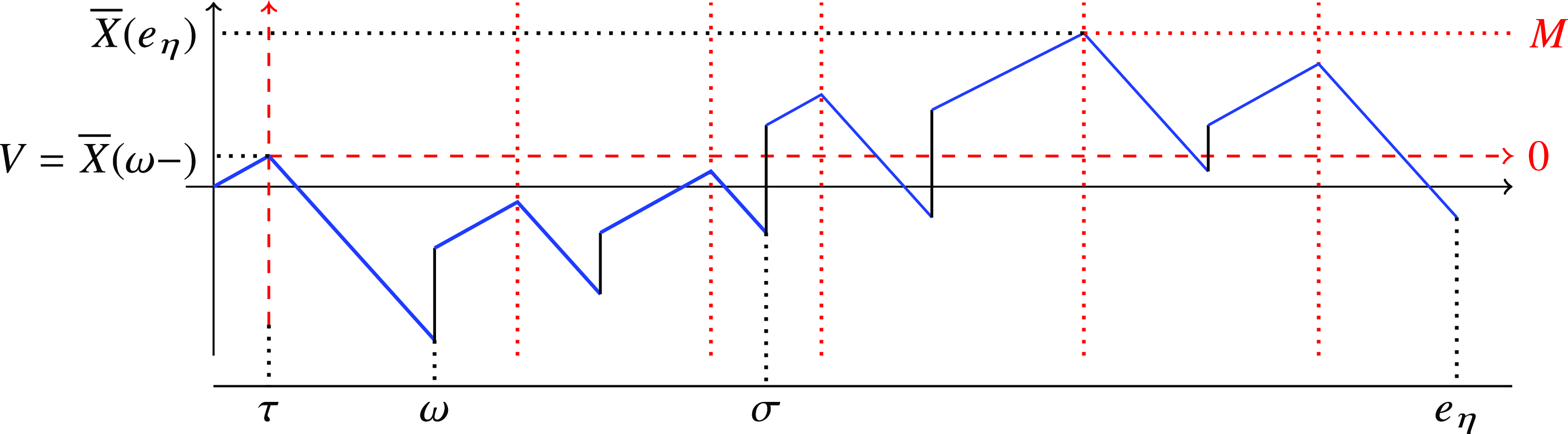
Proof. The argument is illustrated schematically in Figure 4. It uses the alternative dashed coordinate system where the dotted red vertical lines divide the process into segments starting with a downward move with distribution sized as the displacement
 $D(\omega)$
of Z from
 $\overline X(\omega)$
and is followed by an independent upward move with the stated distribution of
 $U_i$
. The overshoot over
 $\overline X(\omega)$
is simply the overshoot over 0 of the RW with increments distributed as the increments over a section. Since
 $U_i$
has property (R) by Lemma 6.2, the overshoot can be calculated according to Proposition 6.1, which also immediately gives
 $\upsilon=\psi$
and the convergence.
The random walk connection.

Lemma 6.3 The sets
 $(\boldsymbol{\alpha}_i,{\boldsymbol{S}}_i,{\boldsymbol{s}}_i)$
,
 $i=1,2,3$
, given by
 \begin{alignat*}{3} \boldsymbol{\alpha}_1 & = (1\,\,0\,\,\boldsymbol{0}_{1:p}\,\,0), \qquad & {\boldsymbol{S}}_1 & = \left(\begin{array}{l@{\quad}l@{\quad}l} -\delta & \delta\beta_0 & \delta\boldsymbol{\beta}_{1:p} \\ 0 & \delta(1-\beta_0) & \delta\boldsymbol{\beta}_{1:p} \\ \boldsymbol{0}_{1:p}^\top & \boldsymbol{t} & \boldsymbol{T} \end{array} \right), & {\boldsymbol{s}}_1 & = \left(\begin{array}{l} \delta(1-\boldsymbol{\beta}\boldsymbol{1}) \\ \delta(1-\boldsymbol{\beta}\boldsymbol{1}) \\ \boldsymbol{0} \end{array} \right), \\ \boldsymbol{\alpha}_2 & = (0\,\,1\,\,\boldsymbol{0}_{1:p}\quad0), & {\boldsymbol{S}}_2 & = \left(\begin{array}{c@{\quad}c@{\quad}c} 0 & 0 & \boldsymbol{0}_{1:p} \\ 0 & -\delta(1-\beta_0) & \delta\boldsymbol{\beta}_{1:p} \\ \boldsymbol{0}_{1:p}^\top & \boldsymbol{t} & \boldsymbol{T} \end{array} \right), \qquad & {\boldsymbol{s}}_2 & = \begin{pmatrix} 0 \\ \delta(1-\boldsymbol{\beta}\boldsymbol{1}) \\ \boldsymbol{0} \end{pmatrix}, \\ \boldsymbol{\alpha}_3 & = (1\,\,\boldsymbol{0}_{1:p}\,\,0), & {\boldsymbol{S}}_3 & = \left(\begin{array}{c@{\quad}c} -\delta(1-\beta_0) & \delta\boldsymbol{\beta}_{1:p} \\ \boldsymbol{t} & \boldsymbol{T} \end{array} \right), & {\boldsymbol{s}}_3 & = \begin{pmatrix} \delta(1-\boldsymbol{\beta}\boldsymbol{1}) \\ \boldsymbol{0} \end{pmatrix} \end{alignat*}
all represent the same ME distribution.
Proof. Consider the movement of a particle with marks a,b,c,d, where marks a and b indicate an Exp
 $(\delta)$
part of the movement, mark c an ME
 $(\boldsymbol{\alpha},\boldsymbol{T},\boldsymbol{t})$
one, and d that the movement has stopped. The
 $i=1$
representation then models the total length L travelled if the particle starts with mark a and after the Exp
 $(\delta)$
time takes mark b with probability
 $\beta_0$
, mark d with probability
 $1-\beta_0$
, and otherwise mark c. The behaviour with mark b is exactly the same, and after a mark c time, the particle takes mark b. But this does not differ from the movement starting with mark b, which is the one modeled by the
 $i=2$
representation. Since the evolvement of marks does not influence L, representations 1 and 2 therefore give the same distribution of L. That representation 3 also does follows from
 \[ \mathrm{e}^{{\boldsymbol{S}}_2 x} = \left(\begin{array}{l@{\quad}l} 1 & \boldsymbol{0}_{1:p} \\ \boldsymbol{0}_{1:p}^\top & \mathrm{e}^{{\boldsymbol{S}}_3 x} \end{array} \right). \]
Alternatively, we could prove equality of the Laplace transforms
 $\boldsymbol{\alpha}_i(\theta\boldsymbol{I}-{\boldsymbol{S}}_i)^{-1}{\boldsymbol{s}}_i$
by using the formula in [Reference Bladt and Nielsen11, p. 711] for the inverse of a block partitioned matrix.
Proof of Theorem
6.1. We use that
 $\overline X(e_\eta)=V+M$
, where M is the maximum of the random walk in Corollary 6.1 and its proof, cf. Figure 4, and an independent Exp
 $(\delta)$
r.v. The ladder height distribution of this random walk was computed in Corollary 6.1, and we can then appeal to [Reference Bladt and Nielsen11, Theorem 6.2.6, p. 372] to conclude that
 $M \sim \operatorname{ME}_{p+1}(\boldsymbol{\beta},{\boldsymbol{S}}_0+{\boldsymbol{s}}_0\boldsymbol{\beta}, (1-\boldsymbol{\beta}\boldsymbol{1}){\boldsymbol{s}}_0)$
with
 ${\boldsymbol{S}}_0$
and
 ${\boldsymbol{s}}_0$
as in (6.1). This gives the
 $i=1$
representation of the distribution of
 $\overline X(e_\eta)=V+M$
in Lemma 6.3. Now just notice that the
 $i=3$
representation is the one stated in Theorem 6.1. That
 $\boldsymbol{\beta}$
solves the fixed point equation and that the iteration converges was established in Corollary 6.1.
Similarly to the proof of Theorem 6.1 but easier, we have the following analogue of Theorem 3.1.
Theorem 6.2 Assume in (1.2) that
 $-Z$
is a subordinator and Y is
 $\operatorname{CP}(\lambda,H)$
, with H being
 $\operatorname{ME}_p(\boldsymbol{\alpha},\boldsymbol{T},\boldsymbol{t})$
with
 $\boldsymbol{t}=-\boldsymbol{T}\boldsymbol{1}$
and satisfying (R). Then
 $\overline X(e_\eta)$
restricted to
 $(0,\infty)$
is
 $\operatorname{ME}_p(\boldsymbol{\beta}, \boldsymbol{G}(\boldsymbol{\beta})$
,
 $\boldsymbol{g}(\boldsymbol{\beta}))$
, where
 $\boldsymbol{G}(\boldsymbol{\beta})=\boldsymbol{T}+\boldsymbol{t}\boldsymbol{\beta}$
,
 $\boldsymbol{g}(\boldsymbol{\beta})=-\boldsymbol{G}(\boldsymbol{\beta})\boldsymbol{1}$
. Here,
 $\boldsymbol{\beta}$
solves
 $\boldsymbol{\beta}=\psi(\boldsymbol{\beta})$
where
 \begin{align*} \psi(\boldsymbol{\beta}) = \lambda\boldsymbol{\alpha} ((\lambda+\eta)\boldsymbol{I}-\kappa_Z(-\boldsymbol{G}(\boldsymbol{\beta})))^{-1}. \end{align*}
Further,
 $\overline X(e_\eta)$
has an atom of size
 $1-\boldsymbol{\beta}\boldsymbol{1}$
at 0.
The row vector
 $\boldsymbol{\beta}$
can be computed by iteration,
 $\boldsymbol{\beta}^{(n)}\to \boldsymbol{\beta}$
, where
 $\boldsymbol{\beta}^{(n)}=\psi\bigl(\boldsymbol{\beta}^{(n-1)}\bigr)$
and
 $\boldsymbol{\beta}^{(0)}=\boldsymbol{0}$
.
7. Remarks
In exponential Lévy models in finance, the price of a barrier option with fixed maturity T is an integral in the joint distribution of either
 $\overline X(T), X(T)$
or
 $\underline X(T), X(T)$
. In the case of, say,
 $\overline X(T), X(T)$
, this is obviously given by the joint distribution of
 $\overline X(T),D(T)$
(note that
 $X(T)=\overline X(T)-D(T)$
). However, Theorems (3.1) and (4.1) determine the bivariate Laplace transform, characteristic function, etc. with respect to T of
 $\overline X(T),D(T)$
. The price can thus be computed by transform inversion. This or closely related procedures have been implemented, e.g., in [Reference Jeannin and Pistorius18]. For an alternative, using an extension of the present paper to an Erlangian rather than exponential horizon, see [Reference Asmussen6].
Similar transform inversion approaches have been used e.g. in [Reference Deelstra and Simon14] and references therein for European options. For a call option with strike
 $K>S_0$
where
 $S_0$
is the spot price, this involves only the distribution of the positive part
 $X(T)^+$
of X(T).
Corollary 7.1. In the model of the present paper, the distribution of
 $X(e_\eta)^+$
is defective PH with generator
 $\boldsymbol{G}$
and initial vector
 $\boldsymbol{\beta}\mathbb{E}\mathrm{e}^{\boldsymbol{G}D(e_\eta)}$
when Z is a subordinator. Here,
 \[ \mathbb{E}\mathrm{e}^{\boldsymbol{G}D(e_\eta)} = -\eta(\eta\boldsymbol{I}-\kappa(-\boldsymbol{G}))^{-1} ((\boldsymbol{\beta}\otimes\boldsymbol{I})(\boldsymbol{G}\otimes\boldsymbol{I} - \boldsymbol{I}\otimes\boldsymbol{G})^{-1}(\boldsymbol{g}\otimes\boldsymbol{I}))^{-1}. \]
If Z is not a subordinator, the same holds with
 $\boldsymbol{\beta}$
replaced by
 $\boldsymbol{e}_0$
. The formulas also hold in the ME case.
Proof. For
 $x>0$
,
 \begin{align*} \mathbb{P}(X^+(e_\eta)\in\mathrm{d}x) & = \int_0^\infty\mathbb{P}(D(e_\eta)\in\mathrm{d}y)\mathbb{P}(\overline X(\omega)\in\mathrm{d}(x+y) \\ & = \int_0^\infty{\boldsymbol{\beta}}\mathbb{P}(D(e_\eta)\in\mathrm{d}y) \mathrm{e}^{\boldsymbol{G}(x+y)}\boldsymbol{g} = {\boldsymbol{\beta}}\mathbb{E}\mathrm{e}^{{\boldsymbol{G}}D(e_\eta)}\mathrm{e}^{\boldsymbol{G}x}\boldsymbol{g}. \end{align*}
For the expression for
 $\mathbb{E}\mathrm{e}^{\boldsymbol{G}D(e_\eta)}$
, just use the WH identity
 $\mathbb{E}\mathrm{e}^{-\boldsymbol{G} X(e_\eta)} = \mathbb{E}\mathrm{e}^{-\boldsymbol{G}\overline X(e_\eta)}\mathbb{E}\mathrm{e}^{\boldsymbol{G}D(e_\eta)}$
together with
 \begin{align*} \mathbb{E}\mathrm{e}^{-\boldsymbol{G}\overline X(\omega)} & = \int_0^\infty\boldsymbol{\beta}\mathrm{e}^{\boldsymbol{G}x}\boldsymbol{g} \cdot \mathrm{e}^{-\boldsymbol{G}x}\,\mathrm{d}x \\ & = \int_0^\infty\boldsymbol{\beta}\mathrm{e}^{\boldsymbol{G}x}\boldsymbol{g} \cdot \boldsymbol{I}\mathrm{e}^{-\boldsymbol{G}x}\boldsymbol{I}\,\mathrm{d}x = -(\boldsymbol{\beta}\otimes\boldsymbol{I})(\boldsymbol{G}\otimes\boldsymbol{I} - \boldsymbol{I}\otimes\boldsymbol{G})^{-1}(\boldsymbol{g}\otimes\boldsymbol{I}). \end{align*}
In the barrier option example, transform inversion then applies in the same manner.
Another application of our results is the Poisson sampling setting of [Reference Boxma and Mandjes12] dealing with
 $\overline X_{\eta,\gamma}$
, the maximum of X sampled at Poisson
 $(\gamma)$
epochs before
 $e_\eta$
. It is shown in [Reference Boxma and Mandjes12] that
 $\overline X(e_\eta)$
has the same distribution as the independent sum
 $\overline X_{\eta,\gamma}+\overline X(e_{\eta+\gamma})$
. This is used to derive the transform of
 $\overline X_{\eta,\gamma}$
in the spectrally positive case. It is further shown that
 $X_{\eta,\gamma}$
is defective exponential in the spectrally negative cases. However, our approach extends this result for the spectrally negative case to a PH distribution result in the presence of positive PH/ME jumps.
Corollary 7.2. In the model of the present paper, the distribution of
 $\overline X_{e_\eta,\gamma}$
is defective PH with generator
 $\boldsymbol{G}^\gamma+\boldsymbol{g}^\gamma\boldsymbol{\upsilon}$
and initial vector
 $\boldsymbol{\upsilon}$
. Here,
 $\boldsymbol{G}^\gamma$
is as in Corollary 7.2 with
 $\eta$
replaced by
 $\gamma$
,
 $\boldsymbol{g}^\gamma=-\boldsymbol{G}^\gamma\bf1$
and
 $\boldsymbol{\upsilon}=\lim_{n\to\infty}\boldsymbol{\upsilon}^{(n)}$
, where
 \[ \boldsymbol{\upsilon}^{(n)}=\bf0, \qquad \boldsymbol{\upsilon}^{(n+1)} = \frac{\gamma}{\gamma+\eta}\boldsymbol{\beta}^\gamma \mathbb{E}\exp\{\boldsymbol{G}^\gamma+\boldsymbol{g}^\gamma\boldsymbol{\upsilon}^{(n)})D(e_\gamma)\}, \]
when Z is a subordinator and
 $\boldsymbol{\upsilon}^{(n)}$
is given by the same recursion with
 $\boldsymbol{\beta}^\gamma$
replaced by
 $\boldsymbol{e}_0$
otherwise.
Proof. Clearly,
 $\overline X_{\eta,\gamma}$
is distributed as the maximum of a terminating random walk with increments
 $Y_k$
distributed as
 $X(e_\gamma)= \overline X(e_\gamma)-D(e_\gamma)$
(the killing probability is
 $\mathbb{P}(e_\gamma>e_\eta)=\gamma/(\gamma+\eta)$
). Here,
 $\overline X(e_\gamma)$
is PH with generator
 $\boldsymbol{G}^\gamma$
. Combining with [Reference Asmussen1, Theorem 2.2] for the PH case and [Reference Bladt and Nielsen11, Theorems 6.2.6 and 6.2.8] for the ME case gives the result.
We finally remark that in the case where Z is a sum of BM and downward PH jumps, we can avoid using the somewhat complicated form of
 $\kappa_Z(-\boldsymbol{G})$
by using a variant of the present approach, where
 $\omega$
is redefined as the first upward or downward jump instant before
 $e_\eta$
. This variant is the case
 $q=1$
of [Reference Asmussen6].
Funding information
There are no funding bodies to thank relating to the creation of this article.
Competing interests
There were no competing interests to declare which arose during the preparation or publication process of this article.